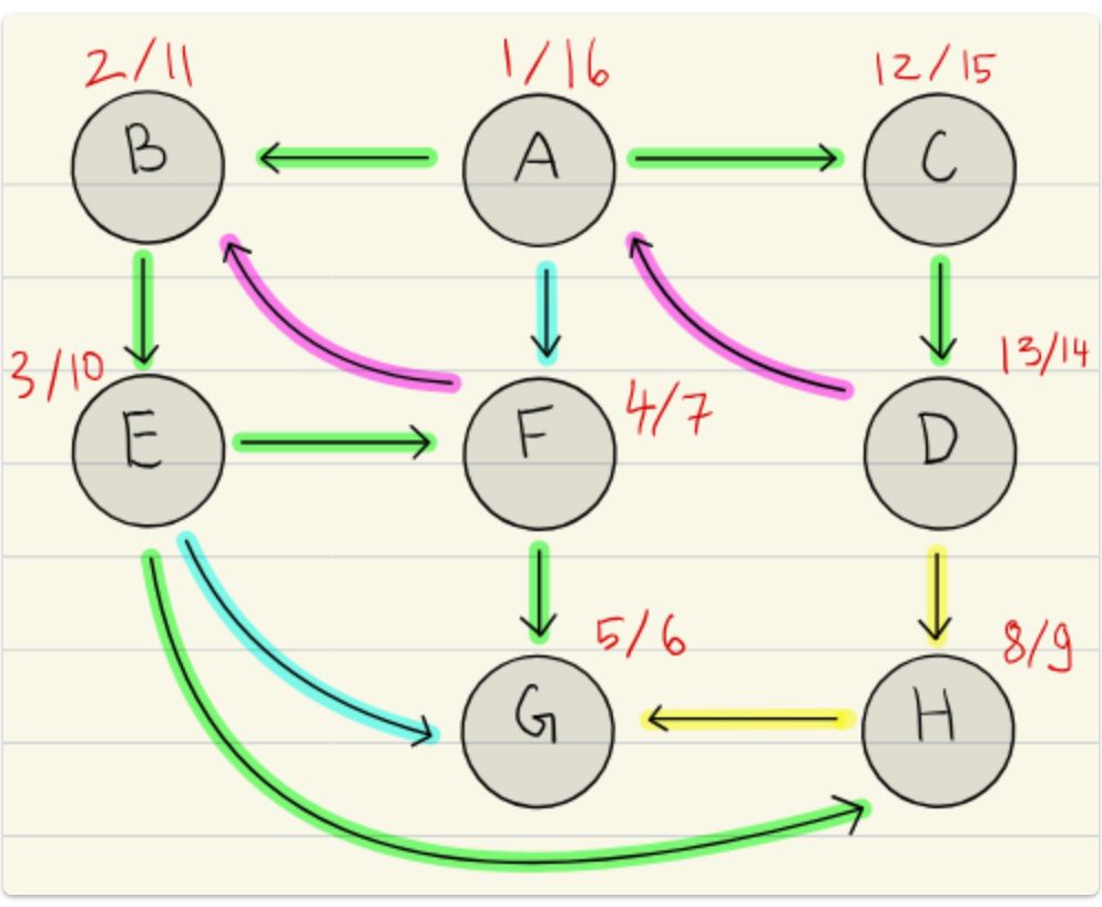
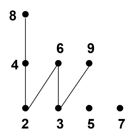
Name the impossible cases in DFS pre/post ordering for edge \((u, v)\):
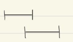
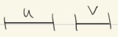
Overlapping but not nested intervals:
{{c2:: \(\text{pre}(u)<\text{pre}(v)<\text{post}(u)<\text{post}(v)\): As visit(u) would call visit(v) before the recursive call ends. }}
Field-by-field Comparison
Field
Before
After
Text
Name the impossible cases in DFS pre/post ordering for edge \((u, v)\):<br><ul><li>{{c1::Overlapping but not Nested Intervals: <img src="paste-b7976dbbff12de2b44594553e0c91633f59e9c05.jpg">}}</li><li>{{c2:: \(\text{pre}(u)<\text{pre}(v)<\text{post}(u)<\text{post}(v)\): <img src="paste-a6fc070f96de8bd2b8148e3891cf956fd611a0a2.jpg"> as visit(u) would call visit(v) before the recursive call ends}}</li></ul>
Name the impossible cases in DFS pre/post ordering for edge \((u, v)\):<br><ul><li>{{c1::Overlapping but not nested intervals: <img src="paste-b7976dbbff12de2b44594553e0c91633f59e9c05.jpg">}}</li><li>{{c2:: \(\text{pre}(u)<\text{pre}(v)<\text{post}(u)<\text{post}(v)\): As visit(u) would call visit(v) before the recursive call ends. <img src="paste-a6fc070f96de8bd2b8148e3891cf956fd611a0a2.jpg"> }}</li></ul>
Let \(W\) be a walk and let \(u\) be a vertex, what is \(\text{deg}_W(u)\)? (generally)
It is the number of edges incident to \(u\) which are part of \(W\) but repetitions are included, therefore it is possible that \(\text{deg}(u) < \text{deg}_W(u)\).
Let \(W\) be a walk and let \(u\) be a vertex, what is \(\text{deg}_W(u)\)? (generally)
The number of edges incident to \(u\) which are part of \(W\) but repetitions are included, therefore it is possible that \(\text{deg}(u) < \text{deg}_W(u)\).
Field-by-field Comparison
Field
Before
After
Back
It is the number of edges incident to \(u\) which are part of \(W\) but <b>repetitions are included</b>, therefore it is possible that \(\text{deg}(u) < \text{deg}_W(u)\).
The number of edges incident to \(u\) which are part of \(W\) but <b>repetitions are included</b>, therefore it is possible that \(\text{deg}(u) < \text{deg}_W(u)\).
DFS Runtime: In a sparse graph adjacency list better, in a dense graph adjacency matrix is better.
\(|E| \geq |V|^2 / 10\), then DFS has the same runtime in the worst-case using adjacency matrices or lists as \(|V| + |E| \leq |V| + |V|^2 \)which is \(O(n^2)\).
In a sparse graph an adjacency list is better, in a dense graph an adjacency matrix is better.
\(|E| \geq |V|^2 / 10\), then DFS has the same runtime in the worst-case using adjacency matrices or lists as \(|V| + |E| \leq |V| + |V|^2 \)which is \(O(n^2)\).
Field-by-field Comparison
Field
Before
After
Text
DFS Runtime: In a sparse graph {{c1:: adjacency list better}}, in a dense graph {{c1:: adjacency matrix is better}}.
Which datastructure is best for DFS?<br><br>In a sparse graph {{c1:: an adjacency list is better}}, in a dense graph {{c1:: an adjacency matrix is better}}.
How can we quickly check whether an Eulerian walk exists?
We can check the degrees of the vertices, an Eulerian walk exists only if at most 2 vertices have an odd degree
This is because if a vertex has an odd degree, it must either be the start point or the endpoint as otherwise we would not be able to leave from it
Field-by-field Comparison
Field
Before
After
Front
How can we quickly check if an Eulerian walk exists?
How can we quickly check whether an Eulerian walk exists?
Back
we can check the degrees of the vertices, an Eulerian walk exists only if at most 2 vertices have an odd degree<br><br>this is because if a vertex has an odd degree, it must either be the start point or the endpoint as otherwise we would not be able to leave from it
We can check the degrees of the vertices, an Eulerian walk exists only if at most 2 vertices have an odd degree<br><br>This is because if a vertex has an odd degree, it must either be the start point or the endpoint as otherwise we would not be able to leave from it
During the recursive call, if we find an adjacent vertex without a post-number, there's a back-edge (\(\implies\)the recursive call for that edge is still active...)
During the recursive call, if we find an adjacent vertex without a post-number, there's a back-edge (\(\implies\)the recursive call for that edge is still active...).
Field-by-field Comparison
Field
Before
After
Front
Check for cycles in DFS algo:
How can we check for cycles via DFS?
Back
During the recursive call, if we find an adjacent vertex <b>without a post-number</b>, there's a back-edge (\(\implies\)the recursive call for that edge is still active...)
During the recursive call, if we find an adjacent vertex <b>without a post-number</b>, there's a back-edge (\(\implies\)the recursive call for that edge is still active...).
The following three statements are equivalent: 1. {{c1::\(\{F_1, \dots, F_k\} \models G\)}} 2. \((F_1 \land F_2 \land \dots F_k) \rightarrow G\) is a tautology 3. {{c3::\(\{F_1, F_2, \dots, F_k, \lnot G\}\) is unsatisfiable}}.
The following three statements are equivalent: 1. {{c1::\(\{F_1, \dots, F_k\} \models G\)}} 2. \((F_1 \land F_2 \land \dots F_k) \rightarrow G\) is a tautology 3. {{c3::\(\{F_1, F_2, \dots, F_k, \lnot G\}\) is unsatisfiable}}.
\((F_1 \land F_2 \land \dots F_k) \rightarrow G\) is a tautology
{{c3::\(\{F_1, F_2, \dots, F_k, \lnot G\}\) is unsatisfiable}}.
This is important for resolution calculus!
Field-by-field Comparison
Field
Before
After
Text
The following three statements are equivalent:<br>1. {{c1::\(\{F_1, \dots, F_k\} \models G\)}}<br>2. {{c2::\((F_1 \land F_2 \land \dots F_k) \rightarrow G\) is a tautology}}<br>3. {{c3::\(\{F_1, F_2, \dots, F_k, \lnot G\}\) is unsatisfiable}}.
The following three statements are equivalent:<br><ol><li>{{c1::\(\{F_1, \dots, F_k\} \models G\)}}</li><li>{{c2::\((F_1 \land F_2 \land \dots F_k) \rightarrow G\) is a tautology}}</li><li>{{c3::\(\{F_1, F_2, \dots, F_k, \lnot G\}\) is unsatisfiable}}.</li></ol>
An axiom \(A\) is a statement taken as true in a theory. Theorems are the statements which follow from .
Field-by-field Comparison
Field
Before
After
Text
An {{c1::<i>axiom</i> \(A\)}} is a {{c2::statement taken as true in a theory}}. {{c3::<i>Theorems</i>}} are the statements which {{c4::follow from these axioms}} (\(A \models T\)).
An {{c1::<i>axiom</i> \(A\)}} is a {{c2::statement taken as true in a theory}}. {{c3::<i>Theorems</i>}} are the statements which {{c4::follow from {{c1::these axioms}} (\(A \models T\))}}.
If a theorem follows from the empty set of axioms \(\emptyset\), then it's a tautology.
This means that it's a theorem in any theory!
Field-by-field Comparison
Field
Before
After
Text
If a theorem follows from the {{c1::empty set}} of axioms \(\emptyset\), then it's a {{c2::<i>tautology</i>}}. This means that {{c3::it's a theorem in any theory!}}
If a theorem follows from the {{c1::empty set of axioms \(\emptyset\)}}, then it's a {{c2::<i>tautology</i>}}. <br><br>This means that {{c3::it's a theorem in any theory!}}
Derivation or inference rule: {{c1::\(\{F_1, \dots, F_k\} \vdash_R G\)}} if {{c2:: \(G\) can be derived from the set \(\{F_1, \dots, F_k\}\) by rule \(R\)}}.
Derivation or inference rule: {{c1::\(\{F_1, \dots, F_k\} \vdash_R G\)}} if {{c2:: \(G\) can be derived from the set \(\{F_1, \dots, F_k\}\) by rule \(R\)}}.
Formally, a derivation rule \(R\) is a relation from the power set of the set of formulas to the set of formulas.
Derivation/inference rule: {{c1::\(\{F_1, \dots, F_k\} \vdash_R G\)::Notation}} if {{c2:: \(G\) can be derived from the set \(\{F_1, \dots, F_k\}\) by rule \(R\)}}.
Derivation/inference rule: {{c1::\(\{F_1, \dots, F_k\} \vdash_R G\)::Notation}} if {{c2:: \(G\) can be derived from the set \(\{F_1, \dots, F_k\}\) by rule \(R\)}}.
Formally, a derivation rule \(R\) is a relation from the power set of the set of formulas to the set of formulas.
Field-by-field Comparison
Field
Before
After
Text
<i>Derivation </i>or <i>inference</i> rule: <br>{{c1::\(\{F_1, \dots, F_k\} \vdash_R G\)}} if {{c2:: \(G\) can be derived from the set \(\{F_1, \dots, F_k\}\) by rule \(R\)}}.
<i>Derivation/</i><i>inference</i> rule: <br>{{c1::\(\{F_1, \dots, F_k\} \vdash_R G\)::Notation}} if {{c2:: \(G\) can be derived from the set \(\{F_1, \dots, F_k\}\) by rule \(R\)}}.
The application of a derivation rule \(R\) to a set \(M\) of formulas means: 1. Select a subset \(N\) of \(M\) such that \(N \vdash_R G\) for some formula \(G\) 2. {{c2::Add \(G\) to the set \(M\) (i.e., replace \(M\) by \(M \cup \{G\}\))}}
The application of a derivation rule \(R\) to a set \(M\) of formulas means: 1. Select a subset \(N\) of \(M\) such that \(N \vdash_R G\) for some formula \(G\) 2. {{c2::Add \(G\) to the set \(M\) (i.e., replace \(M\) by \(M \cup \{G\}\))}}
The application of a derivation rule \(R\) to a set \(M\) of formulas means:
Select a subset \(N\) of \(M\) such that \(N \vdash_R G\) for some formula \(G\)
{{c2::Add \(G\) to the set \(M\) (i.e., replace \(M\) by \(M \cup \{G\}\))}}
Field-by-field Comparison
Field
Before
After
Text
The <i>application of a derivation rule</i> \(R\) to a set \(M\) of formulas means:<br>1. {{c1::Select a subset \(N\) of \(M\) such that \(N \vdash_R G\) for some formula \(G\)}}<br>2. {{c2::Add \(G\) to the set \(M\) (i.e., replace \(M\) by \(M \cup \{G\}\))}}
The <i>application of a derivation rule</i> \(R\) to a set \(M\) of formulas means:<br><ol><li>{{c1::Select a subset \(N\) of \(M\) such that \(N \vdash_R G\) for some formula \(G\)}}</li><li>{{c2::Add \(G\) to the set \(M\) (i.e., replace \(M\) by \(M \cup \{G\}\))}}</li></ol>
Let \(\beta_i = a(\alpha_i)\) for \(i = 1, \dots, d+1\) where Then \(\alpha_i\) distinct for all \(i.\)
\(a(x)\) is given by Lagrange's Interpolation formula: \[a(x) = \sum_{i=1}^{d+1} \beta_i u_i(x)\] where the polynomial \(u_i(x)\) is: \[u_i(x) = \frac{(x - \alpha_1) \cdots (x - \alpha_{i-1})(x - \alpha_{i+1}) \cdots (x - \alpha_{d+1})}{(\alpha_i - \alpha_1) \cdots (\alpha_i - \alpha_{i-1})(\alpha_i - \alpha_{i+1}) \cdots (\alpha_i - \alpha_{d+1})}\]
Note that for \(u_i(x)\) to be well-defined, all constant terms \(\alpha_i - \alpha_j\) in the denominator must be invertible. This is guaranteed in a field since \(\alpha_i - \alpha_j \neq 0\) for \(i \neq j\) (as they are all distinct).
How is Lagrange interpolation for polynomials in a field defined?
Let \(\beta_i = a(\alpha_i)\) for \(i = 1, \dots, d+1\) where Then \(\alpha_i\) distinct for all \(i.\)
\(a(x)\) is given by Lagrange's Interpolation formula: \[a(x) = \sum_{i=1}^{d+1} \beta_i u_i(x)\] where the polynomial \(u_i(x)\) is: \[u_i(x) = \frac{(x - \alpha_1) \cdots (x - \alpha_{i-1})(x - \alpha_{i+1}) \cdots (x - \alpha_{d+1})}{(\alpha_i - \alpha_1) \cdots (\alpha_i - \alpha_{i-1})(\alpha_i - \alpha_{i+1}) \cdots (\alpha_i - \alpha_{d+1})}\]
Note that for \(u_i(x)\) to be well-defined, all constant terms \(\alpha_i - \alpha_j\) in the denominator must be invertible. This is guaranteed in a field since \(\alpha_i - \alpha_j \neq 0\) for \(i \neq j\) (as they are all distinct).
Field-by-field Comparison
Field
Before
After
Front
<p>Lagrange Interpolation for polynomials in a field</p>
<p>How is Lagrange interpolation for polynomials in a field defined?</p>
Orthogonal matrices preserve the norm and inner product of vectors.
In other words, if \(Q \in \mathbb{R}^{n \times n}\) is orthogonal, then, for all \(x, y \in \mathbb{R}^n\) \[ ||Qx|| = ||x|| \text{ and } (Qx)^\top(Qy) = x^\top y \]
Orthogonal matrices preserve the norm and inner product of vectors.
In other words, if \(Q \in \mathbb{R}^{n \times n}\) is orthogonal, then, for all \(x, y \in \mathbb{R}^n\):
\[ ||Qx|| = ||x|| \text{ and } (Qx)^\top(Qy) = x^\top y \]
Field-by-field Comparison
Field
Before
After
Extra
In other words, if \(Q \in \mathbb{R}^{n \times n}\) is orthogonal, then, for all \(x, y \in \mathbb{R}^n\)\[ ||Qx|| = ||x|| \text{ and } (Qx)^\top(Qy) = x^\top y \]<br>
In other words, if \(Q \in \mathbb{R}^{n \times n}\) is orthogonal, then, for all \(x, y \in \mathbb{R}^n\):<br><br>\[ ||Qx|| = ||x|| \text{ and } (Qx)^\top(Qy) = x^\top y \]<br>
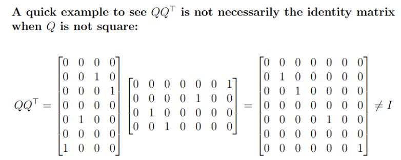
\(QQ^\top = I\) hold? No, the identity has holes on the diagonal.
Field-by-field Comparison
Field
Before
After
Text
If \(Q\) orthogonal is not square does:<br><ul><li>\(Q^\top Q = I\) hold? {{c1:: yes}}</li><li>\(QQ^\top = I\) hold? {{c2:: no, the identity has holes on the diagonal}}</li></ul>
If \(Q\) orthogonal is not square does:<br><ul><li>\(Q^\top Q = I\) hold? {{c1:: Yes.}}</li><li>\(QQ^\top = I\) hold? {{c2:: No, the identity has holes on the diagonal.}}</li></ul>
Let \(Q\) be the \(m \times n\) matrix whose columns are an orthonormal basis of \(C(A)\).
Then the projection matrix that projects to \(C(A)\) is given by \(QQ^\top\). Proof Included
\(A^\top A\) simplifies to \(I\) in the case where our \(A\) is orthogonal. Thus \(P = A (A^\top A)^{-1} A^\top\) simplifies to \(P = AA^\top\).
Field-by-field Comparison
Field
Before
After
Text
<div> Let \(Q\) be the \(m \times n\) matrix whose columns are an orthonormal basis of \(A\).</div><div><br></div><div>Then the projection matrix that projects to \(C(A)\) is given by {{c1:: \(QQ^\top\)}}. <i>Proof Included</i></div>
<div>Let \(Q\) be the \(m \times n\) matrix whose columns are an orthonormal basis of \(C(A)\).</div><div><br></div><div>Then the projection matrix that projects to \(C(A)\) is given by {{c1::\(QQ^\top\)}}. <i>Proof Included</i></div>
We know that \(\forall x \in \mathbb{R}^n\), there exist \(x_0 \in N(A)\) and \(x_1 \in R(A)\) such that \(x = x_0 + x_1 \) and \(x_1^\top x_0 = 0\) as \(N(A) = C(A^\top)^\perp\) are orthogonal complements.
We know that \(\forall x \in \mathbb{R}^n\), there exist \(x_0 \in N(A)\) and \(x_1 \in R(A)\) such that \(x = x_0 + x_1 \) and \(x_1^\top x_0 = 0\) as \(N(A) = C(A^\top)^\perp\) are orthogonal complements.
We know that \(\forall x \in \mathbb{R}^n\), there exist \(x_0 \in N(A)\) and \(x_1 \in R(A)\) such that \(x = x_0 + x_1 \) and \(x_1^\top x_0 = 0\) as \(N(A) = C(A^\top)^\perp\) are orthogonal complements.
We know that \(\forall x \in \mathbb{R}^n\), there exist \(x_0 \in N(A)\) and \(x_1 \in R(A)\) such that \(x = x_0 + x_1 \) and \(x_1^\top x_0 = 0\) as \(N(A) = C(A^\top)^\perp\) are orthogonal complements.
Field-by-field Comparison
Field
Before
After
Text
We know that \(\forall x \in \mathbb{R}^n\), there exist {{c1::\(x_0 \in N(A)\)}} and {{c1::\(x_1 \in R(A)\)}} such that \(x = {{c1:: x_0 + x_1 }}\) and {{c1::\(x_1^\top x_0 = 0\)}} as {{c1::\(N(A) = C(A^\top)^\perp\) are orthogonal complements}}.
We know that \(\forall x \in \mathbb{R}^n\), there exist {{c1::\(x_0 \in N(A)\)}} and {{c1::\(x_1 \in R(A)\)}} such that \(x = {{c2:: x_0 + x_1 }}\) and {{c3::\(x_1^\top x_0 = 0\)}} as {{c3::\(N(A) = C(A^\top)^\perp\) are orthogonal complements}}.
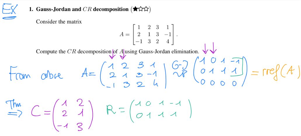
For \(R\) result of RREF on \(A\), \(R\) in \(\text{RREF}(j_1, j_2, \dots, j_r)\) where \(R = \begin{bmatrix} R’ \in r \times n \\ 0 \in (m - r) \times n \end{bmatrix}\).
This \(R’\) is the \(R’\) from the CR decomposition (non-zero rows).
And \(C\) is the submatrix taking only \(j_1, j_2, \dots, j_r\) (independent columns).
Certificate of no solutions:\[ \{x \in \mathbb{R}^n \ | \ Ax = b \} = \emptyset\]is equivalent to
\[{{c1:: \{z \in \mathbb{R}^m \ | \ A^\top z = 0, b^\top z = 1 \} \not = \emptyset }}\]
Note that we don’t need it to be \(1\), it just has to be \(\neq 0\).
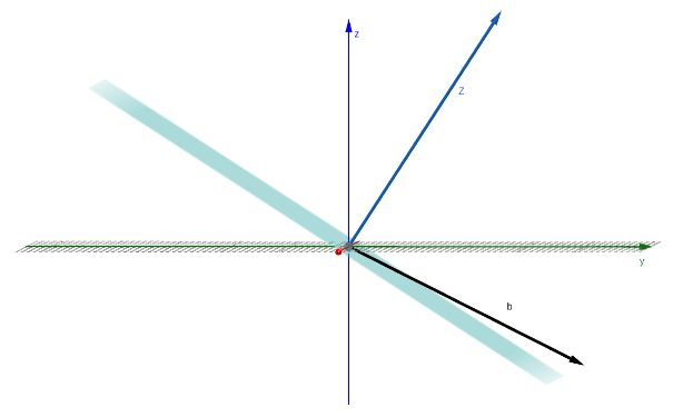
In words: our LSE \(Ax = b\) does not have any solutions if and only if there exists a vector \(z\) that is orthogonal to all columns of \(A\) but not orthogonal to \(b\).
The blue vector \(z\) is orthogonal to all in \(C(A)\), the blue subspace. If \(b\) is not orthogonal to \(z\), this means that it cannot possibly be in the subspace, it must be slightly above/below it. Therefore \(b \not \in C(A)\) and thus there's no solution.
Certificate of no solutions:\[ \{x \in \mathbb{R}^n \ | \ Ax = b \} = \emptyset\]is equivalent to:
\[{{c1:: \{z \in \mathbb{R}^m \ | \ A^\top z = 0, b^\top z = 1 \} \not = \emptyset }}\]
Note that we don’t need it to be \(1\), it just has to be \(\neq 0\).
In words: our LSE \(Ax = b\) does not have any solutions if and only if there exists a vector \(z\) that is orthogonal to all columns of \(A\) but not orthogonal to \(b\).
The blue vector \(z\) is orthogonal to all in \(C(A)\), the blue subspace. If \(b\) is not orthogonal to \(z\), this means that it cannot possibly be in the subspace, it must be slightly above/below it. Therefore \(b \not \in C(A)\) and thus there's no solution.
Field-by-field Comparison
Field
Before
After
Text
<div><b>Certificate</b> of no solutions:\[ \{x \in \mathbb{R}^n \ | \ Ax = b \} = \emptyset\]is <b>equivalent to</b> </div>\[{{c1:: \{z \in \mathbb{R}^m \ | \ A^\top z = 0, b^\top z = 1 \} \not = \emptyset }}\]<div>Note that we don’t need it to be \(1\), it just has to be \(\neq 0\).</div>
<div><b>Certificate</b> of no solutions:\[ \{x \in \mathbb{R}^n \ | \ Ax = b \} = \emptyset\]is <b>equivalent to:</b></div><br>\[{{c1:: \{z \in \mathbb{R}^m \ | \ A^\top z = 0, b^\top z = 1 \} \not = \emptyset }}\]<div>Note that we don’t need it to be \(1\), it just has to be \(\neq 0\).</div>
Let \(A \in \mathbb{R}^{m \times n}\). Let \(x, y \in C(A^\top)\). We have that \[ Ax = Ay \Leftrightarrow x = y \]
This is because \(x, y\) have unique decompositions into the two fundamental subspaces. \[ Ax = Ay \Leftrightarrow x - y \in N(A) \Leftrightarrow \](this holds as \(\implies A(x - y) = 0\)).\[x^\top(x - y) = 0 = y^\top(x - y) \Leftrightarrow\]because of orthogonality of the subspaces\[ (x - y)^\top(x - y) = 0 \]and from this follows that \(||x - y||^2 = 0 \implies x - y = 0\).
Let \(A \in \mathbb{R}^{m \times n}\) and \(x, y \in C(A^\top)\).
We have: \[ Ax = Ay \Leftrightarrow x = y \]
This is because \(x, y\) have unique decompositions into the two fundamental subspaces. \[ Ax = Ay \Leftrightarrow x - y \in N(A) \Leftrightarrow \](this holds as \(\implies A(x - y) = 0\)).
\[x^\top(x - y) = 0 = y^\top(x - y) \Leftrightarrow\]because of orthogonality of the subspaces\[ (x - y)^\top(x - y) = 0 \]and from this follows that \(||x - y||^2 = 0 \implies x - y = 0\).
Field-by-field Comparison
Field
Before
After
Text
Let \(A \in \mathbb{R}^{m \times n}\). Let \(x, y \in C(A^\top)\). We have that \[ {{c1::Ax = Ay}} \Leftrightarrow {{c2:: x = y }}\]
Let \(A \in \mathbb{R}^{m \times n}\) and \(x, y \in C(A^\top)\). <br><br>We have: \[ {{c1::Ax = Ay}} \Leftrightarrow {{c2:: x = y }}\]
Extra
This is because \(x, y\) have unique decompositions into the two fundamental subspaces. \[ Ax = Ay \Leftrightarrow x - y \in N(A) \Leftrightarrow \](this holds as \(\implies A(x - y) = 0\)).\[x^\top(x - y) = 0 = y^\top(x - y) \Leftrightarrow\]because of orthogonality of the subspaces\[ (x - y)^\top(x - y) = 0 \]and from this follows that \(||x - y||^2 = 0 \implies x - y = 0\).
This is because \(x, y\) have unique decompositions into the two fundamental subspaces. \[ Ax = Ay \Leftrightarrow x - y \in N(A) \Leftrightarrow \](this holds as \(\implies A(x - y) = 0\)).<br><br>\[x^\top(x - y) = 0 = y^\top(x - y) \Leftrightarrow\]because of orthogonality of the subspaces\[ (x - y)^\top(x - y) = 0 \]and from this follows that \(||x - y||^2 = 0 \implies x - y = 0\).
Vectors \(q_1, \dots, q_n \in \mathbb{R}^m\) are orthonormal if they are orthogonal and have norm \(1\).In other words, for all \(i, j \in \{1, \dots, n\}\) \[ q_i^\top q_j = {{c1::\delta_{ij} }}\]
Vectors \(q_1, \dots, q_n \in \mathbb{R}^m\) are orthonormal if they are orthogonal and have norm \(1\).In other words, for all \(i, j \in \{1, \dots, n\}\) \[ q_i^\top q_j = {{c1::\delta_{ij} }}\]
Vectors \(q_1, \dots, q_n \in \mathbb{R}^m\) are orthonormal if they are orthogonal and have norm \(1\).
In other words, for all \(i, j \in \{1, \dots, n\}\): \[ q_i^\top q_j = {{c1::\delta_{ij} }}\]
Field-by-field Comparison
Field
Before
After
Text
Vectors \(q_1, \dots, q_n \in \mathbb{R}^m\) are orthonormal if {{c1::they are orthogonal and have norm \(1\)}}.In other words, for all \(i, j \in \{1, \dots, n\}\) \[ q_i^\top q_j = {{c1::\delta_{ij} }}\]
Vectors \(q_1, \dots, q_n \in \mathbb{R}^m\) are orthonormal if {{c1::they are orthogonal and have norm \(1\)}}. <br><br>In other words, for all \(i, j \in \{1, \dots, n\}\): \[ q_i^\top q_j = {{c1::\delta_{ij} }}\]
Assume \(A \in \mathbb{R}^{m \times n}\) has linearly independent rows. Since the rows are linearly independent, the only solution to \(z^\top A = 0\) is \(z = 0\). Hence \(z^\top b = 0 \neq 1\).
Assume \(A \in \mathbb{R}^{m \times n}\) has linearly independent rows. Since the rows are linearly independent, the only solution to \(z^\top A = 0\) is \(z = 0\). Hence \(z^\top b = 0 \neq 1\).
Assume \(A \in \mathbb{R}^{m \times n}\) has linearly independent rows.
Since the rows are linearly independent, the only solution to \(z^\top A = 0\) is \(z = 0\). Hence \(z^\top b = 0 \neq 1\).
Thus \(P\) always contains a solution.
Field-by-field Comparison
Field
Before
After
Text
Applications of the Certificate of no solutions:<br><br>Assume \(A \in \mathbb{R}^{m \times n}\) has <b>linearly independent rows</b>.<br>Since {{c1::the rows are linearly independent}}, the only solution to \(z^\top A = 0\) is {{c1:: \(z = 0\)}}. Hence {{c1::\(z^\top b = 0 \neq 1\)}}.<br><br>Thus {{c1::there is always a solution for the \(P\)}}.
Applications of the Certificate of no solutions:<br><br>Assume \(A \in \mathbb{R}^{m \times n}\) has <b>linearly independent rows</b>.<br><br>Since {{c1::the rows are linearly independent}}, the only solution to \(z^\top A = 0\) is {{c2::\(z = 0\)}}. Hence {{c2::\(z^\top b = 0 \neq 1\)}}.<br><br>Thus {{c3::\(P\) always contains a solution}}.
 as visit(u) would call visit(v) before the recursive call ends}}