Die Linearität der Erwartung hält, wenn \(X_1,\ldots,X_n\) vollkommen wurscht ob unabhängig, du dummbatzi sind?
Note 1: ETH::2. Semester::A&W
Deck: ETH::2. Semester::A&W
Note Type: Horvath Cloze
GUID:
modified
Note Type: Horvath Cloze
GUID:
LE!#OdHaHH
Before
Front
Back
Die Linearität der Erwartung hält, wenn \(X_1,\ldots,X_n\) vollkommen wurscht ob unabhängig, du dummbatzi sind?
After
Front
Die Linearität der Erwartung hält wenn \(X_1,\ldots,X_n\) nicht unabhängig, du dummbatzi sind?
Back
Die Linearität der Erwartung hält wenn \(X_1,\ldots,X_n\) nicht unabhängig, du dummbatzi sind?
Field-by-field Comparison
| Field | Before | After |
|---|---|---|
| Text | Die Linearität der Erwartung hält |
Die Linearität der Erwartung hält wenn \(X_1,\ldots,X_n\) {{c1::nicht unabhängig, du dummbatzi}} sind? |
Note 2: ETH::2. Semester::A&W
Deck: ETH::2. Semester::A&W
Note Type: Horvath Cloze
GUID:
modified
Note Type: Horvath Cloze
GUID:
P#e48Dok$?
Before
Front
Paarweise Unabhängigkeit \(\Leftarrow\) Stochastische Unabhängigkeit
Back
Paarweise Unabhängigkeit \(\Leftarrow\) Stochastische Unabhängigkeit
After
Front
Paarweise Unabhängigkeit \(\not\Rightarrow\) aber \(\Leftarrow\) stochastische Unabhängigkeit!
Back
Paarweise Unabhängigkeit \(\not\Rightarrow\) aber \(\Leftarrow\) stochastische Unabhängigkeit!
Field-by-field Comparison
| Field | Before | After |
|---|---|---|
| Text | Paarweise Unabhängigkeit {{c1::\(\ |
Paarweise Unabhängigkeit {{c1::\(\not\Rightarrow\) aber \(\Leftarrow\)}} stochastische Unabhängigkeit! |
Note 3: ETH::2. Semester::A&W
Deck: ETH::2. Semester::A&W
Note Type: Horvath Cloze
GUID:
modified
Note Type: Horvath Cloze
GUID:
PV7-/GzLwe
Before
Front
Die Rekursionsformel des Pascalschen Dreiecks lautet: \[\binom{n}{k} = {{c3::\binom{n-1}{k-1} + \binom{n-1}{k} }}\]
Back
Die Rekursionsformel des Pascalschen Dreiecks lautet: \[\binom{n}{k} = {{c3::\binom{n-1}{k-1} + \binom{n-1}{k} }}\]
Intuition:
Fixiere Element \(x\).
\[\begin{array}{ccccccccc} & & & & 1 \\ & & & 1 & & 1 \\ & & 1 & & 2 & & 1 \\ & 1 & & 3 & & 3 & & 1 \\ 1 & & 4 & & 6 & & 4 & & 1 \end{array}\]Jeder Eintrag = Summe der zwei Einträge schräg darüber.
Z.B.: \(\binom{4}{2} = 6 = \underbrace{\binom{3}{1}}_{3} + \underbrace{\binom{3}{2}}_{3}\)
Fixiere Element \(x\).
- \(x\) dabei → noch \(k-1\) aus \(n-1\) wählen
- \(x\) nicht dabei → alle \(k\) aus \(n-1\) wählen
\[\begin{array}{ccccccccc} & & & & 1 \\ & & & 1 & & 1 \\ & & 1 & & 2 & & 1 \\ & 1 & & 3 & & 3 & & 1 \\ 1 & & 4 & & 6 & & 4 & & 1 \end{array}\]Jeder Eintrag = Summe der zwei Einträge schräg darüber.
Z.B.: \(\binom{4}{2} = 6 = \underbrace{\binom{3}{1}}_{3} + \underbrace{\binom{3}{2}}_{3}\)
After
Front
Rekursion (Pascalsches Dreieck): \(\binom{n}{k} = {{c3::\binom{n-1}{k-1} + \binom{n-1}{k} }}\)
Back
Rekursion (Pascalsches Dreieck): \(\binom{n}{k} = {{c3::\binom{n-1}{k-1} + \binom{n-1}{k} }}\)
Field-by-field Comparison
| Field | Before | After |
|---|---|---|
| Text | Rekursion (Pascalsches Dreieck): \(\binom{n}{k} = {{c3::\binom{n-1}{k-1} + \binom{n-1}{k} }}\) | |
| Extra |
Note 4: ETH::2. Semester::A&W
Deck: ETH::2. Semester::A&W
Note Type: Horvath Cloze
GUID:
modified
Note Type: Horvath Cloze
GUID:
Pp@EGP+L[^
Before
Front
Hopcroft-Karp findet in einem bipartiten Graphen in \(O({{c2::\sqrt{|V|} \cdot |E|}})\) ein maximales Matching.
Back
Hopcroft-Karp findet in einem bipartiten Graphen in \(O({{c2::\sqrt{|V|} \cdot |E|}})\) ein maximales Matching.
After
Front
Hopcroft-Karp findet in einem bipartiten Graphen in {{c1::\(O(\sqrt{|V|} \cdot |E|)\)}} ein maximales Matching.
Back
Hopcroft-Karp findet in einem bipartiten Graphen in {{c1::\(O(\sqrt{|V|} \cdot |E|)\)}} ein maximales Matching.
Field-by-field Comparison
| Field | Before | After |
|---|---|---|
| Text | Hopcroft-Karp findet in einem {{c1::<b>bipartiten |
Hopcroft-Karp findet in einem {{c1::<b>bipartiten Graphen</b>}} in {{c1::\(O(\sqrt{|V|} \cdot |E|)\)}} ein {{c1::maximales Matching}}. |
Note 5: ETH::2. Semester::A&W
Deck: ETH::2. Semester::A&W
Note Type: Horvath Cloze
GUID:
modified
Note Type: Horvath Cloze
GUID:
iYXQ`8[w/]
Before
Front
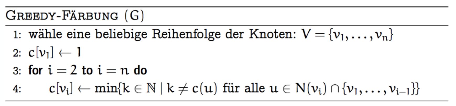
Gilt für die (gewählte) Reihenfolge \(|N(v_i) \cap \{v_1, \ldots, v_{i-1}\}| \leq k\) \(\forall\, 2 \leq i \leq n\), dann benötigt der Greedy-Algorithmus höchstens \(k+1\) viele Farben.
Back
Gilt für die (gewählte) Reihenfolge \(|N(v_i) \cap \{v_1, \ldots, v_{i-1}\}| \leq k\) \(\forall\, 2 \leq i \leq n\), dann benötigt der Greedy-Algorithmus höchstens \(k+1\) viele Farben.
Heuristik:
\(v_n\) := Knoten vom kleinsten Grad. Lösche \(v_n\).
\(v_{n-1}\) := Knoten vom kleinsten Grad im Restgraph. Lösche \(v_{n-1}\). Iteriere.
Falls \(G=(V,E)\) erfüllt:
In jedem Subgraphen gibt es einen Knoten mit Grad \(\leq k\)
\(\Rightarrow\) Heuristik liefert Reihenfolge \(v_1,\ldots,v_n\) für die der Greedy-Algorithmus höchstens \(k+1\) Farben benötigt
After
Front
Gilt für die (gewählte) Reihenfolge \(|N(v_i) \cap \{v_1, \ldots, v_{i-1}\}| \leq k\) \(\forall\, 2 \leq i \leq n\), dann benötigt der Greedy-Algorithmus höchstens \(k+1\) viele Farben.
Proof Included
Back
Gilt für die (gewählte) Reihenfolge \(|N(v_i) \cap \{v_1, \ldots, v_{i-1}\}| \leq k\) \(\forall\, 2 \leq i \leq n\), dann benötigt der Greedy-Algorithmus höchstens \(k+1\) viele Farben.
Proof Included
Heuristik:
\(v_n\) := Knoten vom kleinsten Grad. Lösche \(v_n\).
\(v_{n-1}\) := Knoten vom kleinsten Grad im Restgraph. Lösche \(v_{n-1}\). Iteriere.
Falls \(G=(V,E)\) erfüllt:
In jedem Subgraphen gibt es einen Knoten mit Grad \(\leq k\)
\(\Rightarrow\) Heuristik liefert Reihenfolge \(v_1,\ldots,v_n\) für die der Greedy-Algorithmus höchstens \(k+1\) Farben benötigt
\(v_n\) := Knoten vom kleinsten Grad. Lösche \(v_n\).
\(v_{n-1}\) := Knoten vom kleinsten Grad im Restgraph. Lösche \(v_{n-1}\). Iteriere.
Falls \(G=(V,E)\) erfüllt:
In jedem Subgraphen gibt es einen Knoten mit Grad \(\leq k\)
\(\Rightarrow\) Heuristik liefert Reihenfolge \(v_1,\ldots,v_n\) für die der Greedy-Algorithmus höchstens \(k+1\) Farben benötigt
Field-by-field Comparison
| Field | Before | After |
|---|---|---|
| Text | <img src="paste-abfd33d5257708cb778d485196521618b5c07e9e.jpg"><br><br>Gilt für die (gewählte) Reihenfolge \(|N(v_i) \cap \{v_1, \ldots, v_{i-1}\}| \leq k\) \(\forall\, 2 \leq i \leq n\), dann benötigt der Greedy-Algorithmus höchstens \({{c1::k+1}}\) viele Farben. | <img src="paste-abfd33d5257708cb778d485196521618b5c07e9e.jpg"><br><br>Gilt für die (gewählte) Reihenfolge \(|N(v_i) \cap \{v_1, \ldots, v_{i-1}\}| \leq k\) \(\forall\, 2 \leq i \leq n\), dann benötigt der Greedy-Algorithmus höchstens \({{c1::k+1}}\) viele Farben.<div><br></div><div><i>Proof Included</i></div> |
Note 6: ETH::2. Semester::A&W
Deck: ETH::2. Semester::A&W
Note Type: Horvath Cloze
GUID:
modified
Note Type: Horvath Cloze
GUID:
jc@5=H8@[9
Before
Front
Seien \(A, B\) Ereignisse mit \(\Pr[B] > 0\).
Dann gilt:
\[\Pr[A\mid B] = {{c1::\frac{\Pr[B\mid A] \cdot \Pr[A]}{\Pr[B]}::\text{Bayes} }}.\]
Dann gilt:
\[\Pr[A\mid B] = {{c1::\frac{\Pr[B\mid A] \cdot \Pr[A]}{\Pr[B]}::\text{Bayes} }}.\]
Back
Seien \(A, B\) Ereignisse mit \(\Pr[B] > 0\).
Dann gilt:
\[\Pr[A\mid B] = {{c1::\frac{\Pr[B\mid A] \cdot \Pr[A]}{\Pr[B]}::\text{Bayes} }}.\]
Dann gilt:
\[\Pr[A\mid B] = {{c1::\frac{\Pr[B\mid A] \cdot \Pr[A]}{\Pr[B]}::\text{Bayes} }}.\]
(Satz von Bayes)
Es folgt direkt: \(\Pr[A\mid B] = \frac{\Pr[A \cap B]}{\Pr[B]} = \frac{\Pr[B\mid A]\cdot\Pr[A]}{\Pr[B]}\).
Verallgemeinerung (Partition \(A_1,\ldots,A_n\)):
\(\Pr[A_i\mid B] = \frac{\Pr[B\mid A_i]\Pr[A_i]}{\sum_j \Pr[B\mid A_j]\Pr[A_j]}\).
Es folgt direkt: \(\Pr[A\mid B] = \frac{\Pr[A \cap B]}{\Pr[B]} = \frac{\Pr[B\mid A]\cdot\Pr[A]}{\Pr[B]}\).
Verallgemeinerung (Partition \(A_1,\ldots,A_n\)):
\(\Pr[A_i\mid B] = \frac{\Pr[B\mid A_i]\Pr[A_i]}{\sum_j \Pr[B\mid A_j]\Pr[A_j]}\).
After
Front
Seien \(A, B\) Ereignisse mit \(\Pr[B] > 0\).
Dann gilt:
\[\Pr[A\mid B] = {{c1::\frac{\Pr[B\mid A] \cdot \Pr[A]}{\Pr[B]} }}.\]
Dann gilt:
\[\Pr[A\mid B] = {{c1::\frac{\Pr[B\mid A] \cdot \Pr[A]}{\Pr[B]} }}.\]
Back
Seien \(A, B\) Ereignisse mit \(\Pr[B] > 0\).
Dann gilt:
\[\Pr[A\mid B] = {{c1::\frac{\Pr[B\mid A] \cdot \Pr[A]}{\Pr[B]} }}.\]
Dann gilt:
\[\Pr[A\mid B] = {{c1::\frac{\Pr[B\mid A] \cdot \Pr[A]}{\Pr[B]} }}.\]
(Satz von Bayes)
Es folgt direkt: \(\Pr[A\mid B] = \frac{\Pr[A \cap B]}{\Pr[B]} = \frac{\Pr[B\mid A]\cdot\Pr[A]}{\Pr[B]}\).
Verallgemeinerung (Partition \(A_1,\ldots,A_n\)):
\(\Pr[A_i\mid B] = \frac{\Pr[B\mid A_i]\Pr[A_i]}{\sum_j \Pr[B\mid A_j]\Pr[A_j]}\).
Es folgt direkt: \(\Pr[A\mid B] = \frac{\Pr[A \cap B]}{\Pr[B]} = \frac{\Pr[B\mid A]\cdot\Pr[A]}{\Pr[B]}\).
Verallgemeinerung (Partition \(A_1,\ldots,A_n\)):
\(\Pr[A_i\mid B] = \frac{\Pr[B\mid A_i]\Pr[A_i]}{\sum_j \Pr[B\mid A_j]\Pr[A_j]}\).
Field-by-field Comparison
| Field | Before | After |
|---|---|---|
| Text | Seien \(A, B\) Ereignisse mit \(\Pr[B] > 0\). <br>Dann gilt:<br>\[\Pr[A\mid B] = {{c1::\frac{\Pr[B\mid A] \cdot \Pr[A]}{\Pr[B]} |
Seien \(A, B\) Ereignisse mit \(\Pr[B] > 0\). <br>Dann gilt:<br>\[\Pr[A\mid B] = {{c1::\frac{\Pr[B\mid A] \cdot \Pr[A]}{\Pr[B]} }}.\] |
Note 7: ETH::2. Semester::A&W
Deck: ETH::2. Semester::A&W
Note Type: Horvath Cloze
GUID:
modified
Note Type: Horvath Cloze
GUID:
n.e@Tr+tLx
Before
Front
Stochastische Unabhängigkeit hat zwei äquivalente Formulierungen (falls \(\Pr[B] > 0\)):
- \(\Pr[A \cap B] = \Pr[A] \cdot \Pr[B]\)
- \(\Pr[A\mid B] = \Pr[A]\)
Back
Stochastische Unabhängigkeit hat zwei äquivalente Formulierungen (falls \(\Pr[B] > 0\)):
- \(\Pr[A \cap B] = \Pr[A] \cdot \Pr[B]\)
- \(\Pr[A\mid B] = \Pr[A]\)
Beweis:
Setze 1. in \(\Pr[A\mid B] = \frac{\Pr[A \cap B]}{\Pr[B]}\) ein, dann kürzt sich \(\Pr[B]\) weg.
Intuition:
Das Eintreten von \(B\) beeinflusst die Wahrscheinlichkeit von \(A\) nicht.
Setze 1. in \(\Pr[A\mid B] = \frac{\Pr[A \cap B]}{\Pr[B]}\) ein, dann kürzt sich \(\Pr[B]\) weg.
Intuition:
Das Eintreten von \(B\) beeinflusst die Wahrscheinlichkeit von \(A\) nicht.
After
Front
Falls \(\Pr[B] > 0\) ist stochastische Unabhängigkeit \(\Pr[A \cap B] = \Pr[A] \cdot \Pr[B]\) ident mit \(\Pr[A|B] = \Pr[A]\) (Bayes).
Back
Falls \(\Pr[B] > 0\) ist stochastische Unabhängigkeit \(\Pr[A \cap B] = \Pr[A] \cdot \Pr[B]\) ident mit \(\Pr[A|B] = \Pr[A]\) (Bayes).
Field-by-field Comparison
| Field | Before | After |
|---|---|---|
| Text | Falls \(\Pr[B] > 0\) ist stochastische Unabhängigkeit \(\Pr[A \cap B] = \Pr[A] \cdot \Pr[B]\) ident mit {{c1:: \(\Pr[A|B] = \Pr[A]\) (Bayes)}}. | |
| Extra |
Note 8: ETH::2. Semester::A&W
Deck: ETH::2. Semester::A&W
Note Type: Horvath Cloze
GUID:
modified
Note Type: Horvath Cloze
GUID:
o78LP-Mw-W
Before
Front
Für alle \(k \geq 2\) gibt es einen dreiecksfreien Graphen \(G_k\) mit \(\chi(G_k) \geq k\).
Back
Für alle \(k \geq 2\) gibt es einen dreiecksfreien Graphen \(G_k\) mit \(\chi(G_k) \geq k\).
(Mycielski-Konstruktion)
Konstruktion:
Aus \(G_k = (V_k, E_k)\) mit \(V_k = \{v_1,\ldots,v_n\}\) bilde \(G_{k+1}\):
Füge Knoten \(w_1,\ldots,w_n, z\) hinzu. \(w_i\) ist mit allen Nachbarn von \(v_i\) verbunden (aber nicht mit \(v_i\) selbst). \(z\) ist mit allen \(w_i\) verbunden.
Der neue Graph ist dreiecksfrei und braucht eine Farbe mehr als \(G_k\).
After
Front
Für alle \(k \geq 2\) gibt es einen dreiecksfreien Graphen \(G_k\) mit \(\chi(G_k) \geq k\).
Back
Für alle \(k \geq 2\) gibt es einen dreiecksfreien Graphen \(G_k\) mit \(\chi(G_k) \geq k\).
(Mycielski-Konstruktion)
Konstruktion:
Aus \(G_k = (V_k, E_k)\) mit \(V_k = \{v_1,\ldots,v_n\}\) bilde \(G_{k+1}\):
Füge Knoten \(w_1,\ldots,w_n, z\) hinzu. \(w_i\) ist mit allen Nachbarn von \(v_i\) verbunden (aber nicht mit \(v_i\) selbst). \(z\) ist mit allen \(w_i\) verbunden.
Der neue Graph ist dreiecksfrei und braucht eine Farbe mehr als \(G_k\).
Konstruktion:
Aus \(G_k = (V_k, E_k)\) mit \(V_k = \{v_1,\ldots,v_n\}\) bilde \(G_{k+1}\):
Füge Knoten \(w_1,\ldots,w_n, z\) hinzu. \(w_i\) ist mit allen Nachbarn von \(v_i\) verbunden (aber nicht mit \(v_i\) selbst). \(z\) ist mit allen \(w_i\) verbunden.
Der neue Graph ist dreiecksfrei und braucht eine Farbe mehr als \(G_k\).
Field-by-field Comparison
| Field | Before | After |
|---|---|---|
| Text | Für alle \(k \geq 2\) gibt es einen {{c1::dreiecksfreien}} Graphen \(G_k\) mit \(\chi(G_k) \geq |
Für alle \(k \geq 2\) gibt es einen {{c1::dreiecksfreien}} Graphen \(G_k\) mit \(\chi(G_k) \geq {{c2::k}}\). |
Note 9: ETH::2. Semester::A&W
Deck: ETH::2. Semester::A&W
Note Type: Horvath Cloze
GUID:
modified
Note Type: Horvath Cloze
GUID:
qsXztu}x3_
Before
Front
Ereignisse \(A_1, \ldots, A_n\) heissen stochastisch unabhängig, falls für alle nichtleeren \(I \subseteq \{1,\ldots,n\}\) gilt:
\[{{c2::\Pr\!\left[\bigcap_{i \in I} A_i\right] = \prod_{i \in I} \Pr[A_i]}}.\]
\[{{c2::\Pr\!\left[\bigcap_{i \in I} A_i\right] = \prod_{i \in I} \Pr[A_i]}}.\]
Back
Ereignisse \(A_1, \ldots, A_n\) heissen stochastisch unabhängig, falls für alle nichtleeren \(I \subseteq \{1,\ldots,n\}\) gilt:
\[{{c2::\Pr\!\left[\bigcap_{i \in I} A_i\right] = \prod_{i \in I} \Pr[A_i]}}.\]
\[{{c2::\Pr\!\left[\bigcap_{i \in I} A_i\right] = \prod_{i \in I} \Pr[A_i]}}.\]
Achtung:
Paarweise Unabhängigkeit (\(\Pr[A_i \cap A_j] = \Pr[A_i]\Pr[A_j]\) für alle \(i \neq j\)) impliziert NICHT stochastische Unabhängigkeit!
Paarweise Unabhängigkeit (\(\Pr[A_i \cap A_j] = \Pr[A_i]\Pr[A_j]\) für alle \(i \neq j\)) impliziert NICHT stochastische Unabhängigkeit!
After
Front
Ereignisse \(A_1, \ldots, A_n\) heißen stochastisch unabhängig,
falls für alle nichtleeren \(I \subseteq \{1,\ldots,n\}\) gilt:
\[{{c2::\Pr\!\left[\bigcap_{i \in I} A_i\right] = \prod_{i \in I} \Pr[A_i]}}.\]
falls für alle nichtleeren \(I \subseteq \{1,\ldots,n\}\) gilt:
\[{{c2::\Pr\!\left[\bigcap_{i \in I} A_i\right] = \prod_{i \in I} \Pr[A_i]}}.\]
Back
Ereignisse \(A_1, \ldots, A_n\) heißen stochastisch unabhängig,
falls für alle nichtleeren \(I \subseteq \{1,\ldots,n\}\) gilt:
\[{{c2::\Pr\!\left[\bigcap_{i \in I} A_i\right] = \prod_{i \in I} \Pr[A_i]}}.\]
falls für alle nichtleeren \(I \subseteq \{1,\ldots,n\}\) gilt:
\[{{c2::\Pr\!\left[\bigcap_{i \in I} A_i\right] = \prod_{i \in I} \Pr[A_i]}}.\]
Achtung:
Paarweise Unabhängigkeit (\(\Pr[A_i \cap A_j] = \Pr[A_i]\Pr[A_j]\) für alle \(i \neq j\)) impliziert NICHT stochastische Unabhängigkeit!
Paarweise Unabhängigkeit (\(\Pr[A_i \cap A_j] = \Pr[A_i]\Pr[A_j]\) für alle \(i \neq j\)) impliziert NICHT stochastische Unabhängigkeit!
Field-by-field Comparison
| Field | Before | After |
|---|---|---|
| Text | Ereignisse \(A_1, \ldots, A_n\) hei |
Ereignisse \(A_1, \ldots, A_n\) heißen stochastisch unabhängig,<br>falls für alle nichtleeren \(I \subseteq \{1,\ldots,n\}\) gilt:<br>\[{{c2::\Pr\!\left[\bigcap_{i \in I} A_i\right] = \prod_{i \in I} \Pr[A_i]}}.\] |
Note 10: ETH::2. Semester::A&W
Deck: ETH::2. Semester::A&W
Note Type: Horvath Cloze
GUID:
modified
Note Type: Horvath Cloze
GUID:
s7OsezhA)h
Before
Front
Für den Binomialkoeffizienten gelten:
- \(\binom{n}{0} = 1\)
- \(\binom{n}{n} = 1\)
- \(\binom{n}{1} = n\)
Back
Für den Binomialkoeffizienten gelten:
- \(\binom{n}{0} = 1\)
- \(\binom{n}{n} = 1\)
- \(\binom{n}{1} = n\)
After
Front
Für den Binomialkoeffizienten gelten:
Randfälle: \(\binom{n}{0} = 1\), \(\binom{n}{n} = 1\), \(\binom{n}{1} = n\)
Randfälle: \(\binom{n}{0} = 1\), \(\binom{n}{n} = 1\), \(\binom{n}{1} = n\)
Back
Für den Binomialkoeffizienten gelten:
Randfälle: \(\binom{n}{0} = 1\), \(\binom{n}{n} = 1\), \(\binom{n}{1} = n\)
Randfälle: \(\binom{n}{0} = 1\), \(\binom{n}{n} = 1\), \(\binom{n}{1} = n\)
Field-by-field Comparison
| Field | Before | After |
|---|---|---|
| Text | Für den Binomialkoeffizienten gelten:<br> |
Für den Binomialkoeffizienten gelten:<br>Randfälle: \(\binom{n}{0} = {{c2::1}}\), \(\binom{n}{n} = {{c2::1}}\), \(\binom{n}{1} = {{c2::n}}\) |
Note 11: ETH::2. Semester::A&W
Deck: ETH::2. Semester::A&W
Note Type: Horvath Cloze
GUID:
modified
Note Type: Horvath Cloze
GUID:
tHY-Qji=0u
Before
Front
Zwei Ereignisse \(A\) und \(B\) heißen stochastisch unabhängig, falls:
\[\Pr[A \cap B] = \Pr[A] \cdot \Pr[B] \]
\[\Pr[A \cap B] = \Pr[A] \cdot \Pr[B] \]
Back
Zwei Ereignisse \(A\) und \(B\) heißen stochastisch unabhängig, falls:
\[\Pr[A \cap B] = \Pr[A] \cdot \Pr[B] \]
\[\Pr[A \cap B] = \Pr[A] \cdot \Pr[B] \]
Intuition:
Das Eintreten von \(B\) beeinflusst die Wahrscheinlichkeit von \(A\) nicht.
Das Eintreten von \(B\) beeinflusst die Wahrscheinlichkeit von \(A\) nicht.
After
Front
Zwei Ereignisse \(A\) und \(B\) heißen stochastisch unabhängig, falls
\[\Pr[A \cap B] = \Pr[A] \cdot \Pr[B] \]
\[\Pr[A \cap B] = \Pr[A] \cdot \Pr[B] \]
Back
Zwei Ereignisse \(A\) und \(B\) heißen stochastisch unabhängig, falls
\[\Pr[A \cap B] = \Pr[A] \cdot \Pr[B] \]
\[\Pr[A \cap B] = \Pr[A] \cdot \Pr[B] \]
Intuition:
Das Eintreten von \(B\) beeinflusst die Wahrscheinlichkeit von \(A\) nicht.
Das Eintreten von \(B\) beeinflusst die Wahrscheinlichkeit von \(A\) nicht.
Field-by-field Comparison
| Field | Before | After |
|---|---|---|
| Text | Zwei Ereignisse \(A\) und \(B\) heißen {{c1::stochastisch unabhängig}}, falls |
Zwei Ereignisse \(A\) und \(B\) heißen {{c1::stochastisch unabhängig}}, falls<br>\[{{c2::\Pr[A \cap B] = \Pr[A] \cdot \Pr[B]}} \] |
Note 12: ETH::2. Semester::Analysis
Deck: ETH::2. Semester::Analysis
Note Type: Horvath Cloze
GUID:
modified
Note Type: Horvath Cloze
GUID:
=wRp[:z20n
Before
Front
Sei \(\sum a_n\) {{c1::bedingt konvergent und \(L \in \mathbb{R} \cup \{+\infty, -\infty\}\)}}.
Dann {{c2::gibt es eine Bijektion \(\phi\), so dass:
\[\sum_{n=0}^\infty a_{\phi(n)} = L\]}}
Dann {{c2::gibt es eine Bijektion \(\phi\), so dass:
\[\sum_{n=0}^\infty a_{\phi(n)} = L\]}}
Back
Sei \(\sum a_n\) {{c1::bedingt konvergent und \(L \in \mathbb{R} \cup \{+\infty, -\infty\}\)}}.
Dann {{c2::gibt es eine Bijektion \(\phi\), so dass:
\[\sum_{n=0}^\infty a_{\phi(n)} = L\]}}
Dann {{c2::gibt es eine Bijektion \(\phi\), so dass:
\[\sum_{n=0}^\infty a_{\phi(n)} = L\]}}
(Riemannscher Umordnungssatz)
Merke: Bedingt konvergente Reihen können durch Umordnung jeden Grenzwert annehmen!
Merke: Bedingt konvergente Reihen können durch Umordnung jeden Grenzwert annehmen!
After
Front
Riemannscher Umordnungssatz (bedingt konvergente Reihen): Sei \(\sum a_n\) {{c1::bedingt konvergent und \(L \in \mathbb{R} \cup \{+\infty, -\infty\}\)}}.
Dann {{c2::gibt es eine Bijektion \(\phi\), so dass:
\[\sum_{n=0}^\infty a_{\phi(n)} = L\]}}
Dann {{c2::gibt es eine Bijektion \(\phi\), so dass:
\[\sum_{n=0}^\infty a_{\phi(n)} = L\]}}
Back
Riemannscher Umordnungssatz (bedingt konvergente Reihen): Sei \(\sum a_n\) {{c1::bedingt konvergent und \(L \in \mathbb{R} \cup \{+\infty, -\infty\}\)}}.
Dann {{c2::gibt es eine Bijektion \(\phi\), so dass:
\[\sum_{n=0}^\infty a_{\phi(n)} = L\]}}
Dann {{c2::gibt es eine Bijektion \(\phi\), so dass:
\[\sum_{n=0}^\infty a_{\phi(n)} = L\]}}
Merke: Bedingt konvergente Reihen können durch Umordnung jeden Grenzwert annehmen!
Field-by-field Comparison
| Field | Before | After |
|---|---|---|
| Text | Sei \(\sum a_n\) {{c1::<b>bedingt konvergent</b> und \(L \in \mathbb{R} \cup \{+\infty, -\infty\}\)}}.<br><br>Dann {{c2::gibt es eine Bijektion \(\phi\), so dass:<br>\[\sum_{n=0}^\infty a_{\phi(n)} = L\]}} | <b>Riemannscher</b> Umordnungssatz (bedingt konvergente Reihen): Sei \(\sum a_n\) {{c1::<b>bedingt konvergent</b> und \(L \in \mathbb{R} \cup \{+\infty, -\infty\}\)}}.<br><br>Dann {{c2::gibt es eine Bijektion \(\phi\), so dass:<br>\[\sum_{n=0}^\infty a_{\phi(n)} = L\]}} |
| Extra | <b>Merke:</b> Bedingt konvergente Reihen können durch Umordnung <i>jeden</i> Grenzwert annehmen! |
Note 13: ETH::2. Semester::Analysis
Deck: ETH::2. Semester::Analysis
Note Type: Horvath Cloze
GUID:
modified
Note Type: Horvath Cloze
GUID:
@#Owv2&S1x
Before
Front
Beim Leibniz-Kriterium gilt die Fehlerabschätzung:
\[|S - S_n| \leq {{c1::a_{n+1} }}\]D.h. der Fehler ist höchstens so gross wie der erste weggelassene Term.
\[|S - S_n| \leq {{c1::a_{n+1} }}\]D.h. der Fehler ist höchstens so gross wie der erste weggelassene Term.
Back
Beim Leibniz-Kriterium gilt die Fehlerabschätzung:
\[|S - S_n| \leq {{c1::a_{n+1} }}\]D.h. der Fehler ist höchstens so gross wie der erste weggelassene Term.
\[|S - S_n| \leq {{c1::a_{n+1} }}\]D.h. der Fehler ist höchstens so gross wie der erste weggelassene Term.
Nützlich zur numerischen Approximation alternierender Reihen.
After
Front
Beim Leibniz-Kriterium gilt die Fehlerabschätzung:
\[|S - S_n| \leq {{c1::a_{n+1} }}\]
D.h. der Fehler ist höchstens so groß wie der erste weggelassene Term.
\[|S - S_n| \leq {{c1::a_{n+1} }}\]
D.h. der Fehler ist höchstens so groß wie der erste weggelassene Term.
Back
Beim Leibniz-Kriterium gilt die Fehlerabschätzung:
\[|S - S_n| \leq {{c1::a_{n+1} }}\]
D.h. der Fehler ist höchstens so groß wie der erste weggelassene Term.
\[|S - S_n| \leq {{c1::a_{n+1} }}\]
D.h. der Fehler ist höchstens so groß wie der erste weggelassene Term.
Nützlich zur numerischen Approximation alternierender Reihen.
Field-by-field Comparison
| Field | Before | After |
|---|---|---|
| Text | Beim Leibniz-Kriterium gilt die Fehlerabschätzung:<br>\[|S - S_n| \leq {{c1::a_{n+1} }}\]D.h. der Fehler ist höchstens so gro |
Beim Leibniz-Kriterium gilt die Fehlerabschätzung:<br>\[|S - S_n| \leq {{c1::a_{n+1} }}\]<br>D.h. der Fehler ist höchstens so groß wie {{c1::der erste weggelassene Term}}. |
Note 14: ETH::2. Semester::Analysis
Deck: ETH::2. Semester::Analysis
Note Type: Horvath Cloze
GUID:
modified
Note Type: Horvath Cloze
GUID:
j1*KfG}T{:
Before
Front
Eine Reihe heisst bedingt konvergent, wenn sie konvergiert, aber die Reihe der Beträge \(\sum |a_k|\) divergiert.
Back
Eine Reihe heisst bedingt konvergent, wenn sie konvergiert, aber die Reihe der Beträge \(\sum |a_k|\) divergiert.
(D.h. nicht absolut konvergiert..)
Beispiel:
\(\sum \frac{(-1)^n}{n}\) ist bedingt konvergent.
Beispiel:
\(\sum \frac{(-1)^n}{n}\) ist bedingt konvergent.
After
Front
Eine Reihe heisst bedingt konvergent, wenn sie konvergiert, aber die Reihe der Beträge \(\sum |a_k|\) divergiert.
Counterexample included
Back
Eine Reihe heisst bedingt konvergent, wenn sie konvergiert, aber die Reihe der Beträge \(\sum |a_k|\) divergiert.
Counterexample included
(D.h. nicht absolut konvergiert..)
Beispiel:
\(\sum \frac{(-1)^n}{n}\) ist bedingt konvergent.
Beispiel:
\(\sum \frac{(-1)^n}{n}\) ist bedingt konvergent.
Field-by-field Comparison
| Field | Before | After |
|---|---|---|
| Text | Eine Reihe heisst <b>bedingt konvergent</b>, wenn sie {{c1::konvergiert, aber die Reihe der Beträge \(\sum |a_k|\) divergiert}}. | Eine Reihe heisst <b>bedingt konvergent</b>, wenn sie {{c1::konvergiert, aber die Reihe der Beträge \(\sum |a_k|\) divergiert}}.<div><br></div><div><i>Counterexample included</i></div> |
Note 15: ETH::2. Semester::Analysis
Deck: ETH::2. Semester::Analysis
Note Type: Horvath Classic
GUID:
modified
Note Type: Horvath Classic
GUID:
jKp`Sev.N*
Before
Front
Warum ist jede Cauchy-Folge in \(\mathbb{R}\) konvergent, aber nicht jede in \(\mathbb{Q}\)?
Back
Warum ist jede Cauchy-Folge in \(\mathbb{R}\) konvergent, aber nicht jede in \(\mathbb{Q}\)?
Weil \(\mathbb{R}\) vollständig ist (keine "Lücken"), während \(\mathbb{Q}\) das nicht ist.
Beispiel:
Die Folge \(1,\; 1.4,\; 1.41,\; 1.414,\; \dots\) ist Cauchy in \(\mathbb{Q}\), konvergiert aber gegen \(\sqrt{2} \notin \mathbb{Q}\).
Der Grenzwert existiert in \(\mathbb{Q}\) nicht - die "Lücke" fehlt.
In \(\mathbb{R}\) ist \(\sqrt{2}\) vorhanden, also konvergiert die Folge dort.
Beispiel:
Die Folge \(1,\; 1.4,\; 1.41,\; 1.414,\; \dots\) ist Cauchy in \(\mathbb{Q}\), konvergiert aber gegen \(\sqrt{2} \notin \mathbb{Q}\).
Der Grenzwert existiert in \(\mathbb{Q}\) nicht - die "Lücke" fehlt.
In \(\mathbb{R}\) ist \(\sqrt{2}\) vorhanden, also konvergiert die Folge dort.
After
Front
Warum gilt Cauchy \(\iff\) konvergent in \(\mathbb{R}\), aber nicht in \(\mathbb{Q}\)?
Back
Warum gilt Cauchy \(\iff\) konvergent in \(\mathbb{R}\), aber nicht in \(\mathbb{Q}\)?
In \(\mathbb{R}\): jede Cauchy-Folge konvergiert in \(\mathbb{R}\) (Vollständigkeit).
In \(\mathbb{Q}\): Eine Cauchy-Folge in \(\mathbb{Q}\) kann gegen \(\sqrt{2} \notin \mathbb{Q}\) konvergieren — der Grenzwert liegt außerhalb des Raumes. \(\mathbb{Q}\) ist nicht vollständig.
In \(\mathbb{Q}\): Eine Cauchy-Folge in \(\mathbb{Q}\) kann gegen \(\sqrt{2} \notin \mathbb{Q}\) konvergieren — der Grenzwert liegt außerhalb des Raumes. \(\mathbb{Q}\) ist nicht vollständig.
Field-by-field Comparison
| Field | Before | After |
|---|---|---|
| Front | Warum |
Warum gilt Cauchy \(\iff\) konvergent in \(\mathbb{R}\), aber nicht in \(\mathbb{Q}\)? |
| Back | In \(\mathbb{R}\): jede Cauchy-Folge konvergiert <b>in</b> \(\mathbb{R}\) (Vollständigkeit).<br><br>In \(\mathbb{Q}\): Eine Cauchy-Folge in \(\mathbb{Q}\) kann gegen \(\sqrt{2} \notin \mathbb{Q}\) konvergieren — der Grenzwert liegt außerhalb des Raumes. \(\mathbb{Q}\) ist <b>nicht vollständig</b>. |
Note 16: ETH::2. Semester::Analysis
Deck: ETH::2. Semester::Analysis
Note Type: Horvath Cloze
GUID:
modified
Note Type: Horvath Cloze
GUID:
tRig1dAtan06
Before
Front
Der Wertebereich von \(\arctan\) ist \({{c1::\left(-\frac{\pi}{2},\, \frac{\pi}{2}\right)}}\), und die Funktion ist streng monoton steigend.
Back
Der Wertebereich von \(\arctan\) ist \({{c1::\left(-\frac{\pi}{2},\, \frac{\pi}{2}\right)}}\), und die Funktion ist streng monoton steigend.
After
Front
The range of \(\arctan\) is \({{c1::\left(-\frac{\pi}{2},\, \frac{\pi}{2}\right)}}\), and it is a strictly increasing function.
Back
The range of \(\arctan\) is \({{c1::\left(-\frac{\pi}{2},\, \frac{\pi}{2}\right)}}\), and it is a strictly increasing function.
Field-by-field Comparison
| Field | Before | After |
|---|---|---|
| Text | The range of \(\arctan\) is \({{c1::\left(-\frac{\pi}{2},\, \frac{\pi}{2}\right)}}\), and it is a {{c1::strictly increasing}} function. |
Note 17: ETH::2. Semester::Analysis
Deck: ETH::2. Semester::Analysis
Note Type: Horvath Cloze
GUID:
modified
Note Type: Horvath Cloze
GUID:
u$3f,(&]?[
Before
Front
Absolut konvergent \(\implies\)konvergent
Back
Absolut konvergent \(\implies\)konvergent
nicht andersherum, na no na ned
After
Front
Absolut konvergent \(\implies\) konvergent
Back
Absolut konvergent \(\implies\) konvergent
nicht andersherum
Field-by-field Comparison
| Field | Before | After |
|---|---|---|
| Text | Absolut konvergent \(\implies\){{c |
Absolut konvergent \(\implies\) {{c2::konvergent}} |
| Extra | nicht andersherum |
nicht andersherum |
Note 18: ETH::2. Semester::Analysis
Deck: ETH::2. Semester::Analysis
Note Type: Horvath Cloze
GUID:
modified
Note Type: Horvath Cloze
GUID:
w)NK`}V9nz
Before
Front
Falls \(\sum a_n\) konvergiert, dann gilt zwingend, dass \(\lim_{n\to\infty} a_n = 0\).
Back
Falls \(\sum a_n\) konvergiert, dann gilt zwingend, dass \(\lim_{n\to\infty} a_n = 0\).
Gilt jedoch nicht in die andere Richtung, siehe z.B. die harmonische Reihe \(\sum 1/n\).
After
Front
Falls \(\sum a_n\) konvergiert, dann gilt zwingend: \(\lim_{n\to\infty} a_n = 0\).
Back
Falls \(\sum a_n\) konvergiert, dann gilt zwingend: \(\lim_{n\to\infty} a_n = 0\).
Gegenbeispiel: harmonische Reihe \(\sum 1/n\)
Field-by-field Comparison
| Field | Before | After |
|---|---|---|
| Text | Falls \(\sum a_n\) konvergiert, dann gilt zwingend |
Falls \(\sum a_n\) konvergiert, dann gilt zwingend: \(\lim_{n\to\infty} a_n = {{c1::0}}\). |
| Extra | G |
Gegenbeispiel: harmonische Reihe \(\sum 1/n\) |
Note 19: ETH::2. Semester::Analysis
Deck: ETH::2. Semester::Analysis
Note Type: Horvath Cloze
GUID:
modified
Note Type: Horvath Cloze
GUID:
z>(#?Mm:.A
Before
Front
Wenn \(\sum^\infty a_n\) konvergent ist, gilt:
\[ \sum_{n = 0}^\infty a_n = {{c1::\sum_{n = 0}^{N - 1} a_n + \sum_{n = N}^\infty a_n:: \text{split sum} }}\]
\[ \sum_{n = 0}^\infty a_n = {{c1::\sum_{n = 0}^{N - 1} a_n + \sum_{n = N}^\infty a_n:: \text{split sum} }}\]
Back
Wenn \(\sum^\infty a_n\) konvergent ist, gilt:
\[ \sum_{n = 0}^\infty a_n = {{c1::\sum_{n = 0}^{N - 1} a_n + \sum_{n = N}^\infty a_n:: \text{split sum} }}\]
\[ \sum_{n = 0}^\infty a_n = {{c1::\sum_{n = 0}^{N - 1} a_n + \sum_{n = N}^\infty a_n:: \text{split sum} }}\]
After
Front
Wenn \(\sum^\infty a_n\) konvergent ist gilt:
\[ \sum_{n = 0}^\infty a_n = {{c1::\sum_{n = 0}^{N - 1} + \sum_{n = N}^\infty a_n:: \text{split sum} }}\]
\[ \sum_{n = 0}^\infty a_n = {{c1::\sum_{n = 0}^{N - 1} + \sum_{n = N}^\infty a_n:: \text{split sum} }}\]
Back
Wenn \(\sum^\infty a_n\) konvergent ist gilt:
\[ \sum_{n = 0}^\infty a_n = {{c1::\sum_{n = 0}^{N - 1} + \sum_{n = N}^\infty a_n:: \text{split sum} }}\]
\[ \sum_{n = 0}^\infty a_n = {{c1::\sum_{n = 0}^{N - 1} + \sum_{n = N}^\infty a_n:: \text{split sum} }}\]
Field-by-field Comparison
| Field | Before | After |
|---|---|---|
| Text | Wenn \(\sum^\infty a_n\) konvergent ist |
Wenn \(\sum^\infty a_n\) konvergent ist gilt:<br>\[ \sum_{n = 0}^\infty a_n = {{c1::\sum_{n = 0}^{N - 1} + \sum_{n = N}^\infty a_n:: \text{split sum} }}\] |
Note 20: ETH::2. Semester::Analysis
Deck: ETH::2. Semester::Analysis
Note Type: Horvath Cloze
GUID:
modified
Note Type: Horvath Cloze
GUID:
{XU$eYR/n`
Before
Front
Sei \(0 \leq a_n \leq b_n\) für alle \(n \geq N\):
\(\sum b_n\) konvergiert \(\implies \sum a_n\) konvergiert (Majorante)
\(\sum a_n\) divergiert \(\implies \sum b_n\) divergiert (Minorante)
\(\sum b_n\) konvergiert \(\implies \sum a_n\) konvergiert (Majorante)
\(\sum a_n\) divergiert \(\implies \sum b_n\) divergiert (Minorante)
Back
Sei \(0 \leq a_n \leq b_n\) für alle \(n \geq N\):
\(\sum b_n\) konvergiert \(\implies \sum a_n\) konvergiert (Majorante)
\(\sum a_n\) divergiert \(\implies \sum b_n\) divergiert (Minorante)
\(\sum b_n\) konvergiert \(\implies \sum a_n\) konvergiert (Majorante)
\(\sum a_n\) divergiert \(\implies \sum b_n\) divergiert (Minorante)
Proof:
Da \(\sum_{n=1}^{\infty} b_n\) konvergiert, konvergiert die Folge der Partialsummen. Deswegen ist sie auch beschränkt. Da alle \(a_k \le b_k\), gilt auch \(S_n \le T_n\) (\(S_n\) Partialsummen von \(\sum a_N\), \(T_n\) Partialsummen von \(\sum b_n\)) Dadurch ist auch \(S_n\) beschränkt und da sie monoton steigt (\(a_n \ge 0\)) ist sie auch konvergent. Dadurch ist \(\sum_{n=1}^{\infty} a_n\) konvergent.
Da \(\sum_{n=1}^{\infty} b_n\) konvergiert, konvergiert die Folge der Partialsummen. Deswegen ist sie auch beschränkt. Da alle \(a_k \le b_k\), gilt auch \(S_n \le T_n\) (\(S_n\) Partialsummen von \(\sum a_N\), \(T_n\) Partialsummen von \(\sum b_n\)) Dadurch ist auch \(S_n\) beschränkt und da sie monoton steigt (\(a_n \ge 0\)) ist sie auch konvergent. Dadurch ist \(\sum_{n=1}^{\infty} a_n\) konvergent.
After
Front
Sei \(0 \leq a_n \leq b_n\) für alle \(n \geq N\):
\(\sum b_n\) konvergiert \(\implies \sum a_n \text{ konvergiert}\) (Majorante)
\(\sum a_n\) divergiert \(\implies \sum b_n \text{ divergiert}\) (Minorante)
\(\sum b_n\) konvergiert \(\implies \sum a_n \text{ konvergiert}\) (Majorante)
\(\sum a_n\) divergiert \(\implies \sum b_n \text{ divergiert}\) (Minorante)
Back
Sei \(0 \leq a_n \leq b_n\) für alle \(n \geq N\):
\(\sum b_n\) konvergiert \(\implies \sum a_n \text{ konvergiert}\) (Majorante)
\(\sum a_n\) divergiert \(\implies \sum b_n \text{ divergiert}\) (Minorante)
\(\sum b_n\) konvergiert \(\implies \sum a_n \text{ konvergiert}\) (Majorante)
\(\sum a_n\) divergiert \(\implies \sum b_n \text{ divergiert}\) (Minorante)
Proof:
Da \(\sum_{n=1}^{\infty} b_n\) konvergiert, konvergiert die Folge der Partialsummen. Deswegen ist sie auch beschränkt. Da alle \(a_k \le b_k\), gilt auch \(S_n \le T_n\) (\(S_n\) Partialsummen von \(\sum a_N\), \(T_n\) Partialsummen von \(\sum b_n\)) Dadurch ist auch \(S_n\) beschränkt und da sie monoton steigt (\(a_n \ge 0\)) ist sie auch konvergent. Dadurch ist \(\sum_{n=1}^{\infty} a_n\) konvergent.
Da \(\sum_{n=1}^{\infty} b_n\) konvergiert, konvergiert die Folge der Partialsummen. Deswegen ist sie auch beschränkt. Da alle \(a_k \le b_k\), gilt auch \(S_n \le T_n\) (\(S_n\) Partialsummen von \(\sum a_N\), \(T_n\) Partialsummen von \(\sum b_n\)) Dadurch ist auch \(S_n\) beschränkt und da sie monoton steigt (\(a_n \ge 0\)) ist sie auch konvergent. Dadurch ist \(\sum_{n=1}^{\infty} a_n\) konvergent.
Field-by-field Comparison
| Field | Before | After |
|---|---|---|
| Text | Sei \(0 \leq a_n \leq b_n\) für alle \(n \geq N\):<br><br>\(\sum b_n\) konvergiert \(\implies \sum a_n\) |
Sei \(0 \leq a_n \leq b_n\) für alle \(n \geq N\):<br><br>\(\sum b_n\) konvergiert \(\implies {{c1::\sum a_n \text{ konvergiert}}}\) (<b>Majorante</b>)<br>\(\sum a_n\) divergiert \(\implies {{c2::\sum b_n \text{ divergiert}}}\) (<b>Minorante</b>) |
Note 21: ETH::2. Semester::Analysis
Deck: ETH::2. Semester::Analysis
Note Type: Horvath Cloze
GUID:
modified
Note Type: Horvath Cloze
GUID:
{].oPsIfG|
Before
Front
Exponentialreihe:\[\exp(z) = {{c1:: \sum_{n=0}^\infty \frac{z^n}{n!} }}\]Diese Reihe konvergiert {{c2::absolut für alle \(z \in \mathbb{C}\)::Konvergenztyp}}.
Back
Exponentialreihe:\[\exp(z) = {{c1:: \sum_{n=0}^\infty \frac{z^n}{n!} }}\]Diese Reihe konvergiert {{c2::absolut für alle \(z \in \mathbb{C}\)::Konvergenztyp}}.
(Konvergenzradius \(R = \infty\))
After
Front
Exponentialreihe:\[\exp(z) = {{c1:: \sum_{n=0}^\infty \frac{z^n}{n!} }}\]
Diese Reihe konvergiert {{c1::absolut für alle \(z \in \mathbb{C}\)}} (Konvergenzradius \(R = \infty\)).
Diese Reihe konvergiert {{c1::absolut für alle \(z \in \mathbb{C}\)}} (Konvergenzradius \(R = \infty\)).
Back
Exponentialreihe:\[\exp(z) = {{c1:: \sum_{n=0}^\infty \frac{z^n}{n!} }}\]
Diese Reihe konvergiert {{c1::absolut für alle \(z \in \mathbb{C}\)}} (Konvergenzradius \(R = \infty\)).
Diese Reihe konvergiert {{c1::absolut für alle \(z \in \mathbb{C}\)}} (Konvergenzradius \(R = \infty\)).
Field-by-field Comparison
| Field | Before | After |
|---|---|---|
| Text | Exponentialreihe:\[\exp(z) = {{c1:: \sum_{n=0}^\infty \frac{z^n}{n!} }}\]Diese Reihe konvergiert {{c |
Exponentialreihe:\[\exp(z) = {{c1:: \sum_{n=0}^\infty \frac{z^n}{n!} }}\]<br>Diese Reihe konvergiert {{c1::absolut für alle \(z \in \mathbb{C}\)}} (Konvergenzradius \(R = \infty\)). |
| Extra |
Note 22: ETH::2. Semester::Analysis
Deck: ETH::2. Semester::Analysis
Note Type: Horvath Cloze
GUID:
modified
Note Type: Horvath Cloze
GUID:
}3LSktDYts
Before
Front
Die Riemansche-Zeta Funktion Reihe \(\displaystyle\zeta(s) = {{c1:: \sum_{n=1}^\infty \frac{1}{n^s} }}\) konvergiert für \(s > 1\) und divergiert für \(s\leq1\).
Back
Die Riemansche-Zeta Funktion Reihe \(\displaystyle\zeta(s) = {{c1:: \sum_{n=1}^\infty \frac{1}{n^s} }}\) konvergiert für \(s > 1\) und divergiert für \(s\leq1\).
Oft als Referenzreihe im Vergleichssatz nützlich (wenn Wurzel/Quotient versagen).
After
Front
Die Riemansche-Zeta Funktion Reihe \(\displaystyle\zeta(s) = {{c1:: \sum_{n=1}^\infty \frac{1}{n^s} }}\) konvergiert für \(s > 1\) und divergiert für \(s\leq1\).
Back
Die Riemansche-Zeta Funktion Reihe \(\displaystyle\zeta(s) = {{c1:: \sum_{n=1}^\infty \frac{1}{n^s} }}\) konvergiert für \(s > 1\) und divergiert für \(s\leq1\).
Oft als Referenzreihe im Vergleichssatz nützlich (wenn Wurzel/Quotient versagen).
Field-by-field Comparison
| Field | Before | After |
|---|---|---|
| Text | Die Riemansche-Zeta Funktion Reihe \(\displaystyle\zeta(s) = {{c1:: \sum_{n=1}^\infty \frac{1}{n^s} }}\) konvergiert für {{c |
Die Riemansche-Zeta Funktion Reihe \(\displaystyle\zeta(s) = {{c1:: \sum_{n=1}^\infty \frac{1}{n^s} }}\) konvergiert für {{c1::\(s > 1\)}} und divergiert für {{c1::\(s\leq1\)}}. |
Note 23: ETH::2. Semester::DDCA
Deck: ETH::2. Semester::DDCA
Note Type: Horvath Cloze
GUID:
modified
Note Type: Horvath Cloze
GUID:
jgnr@Obi8f
Before
Front
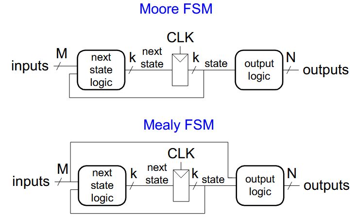
Two types of finite state machines differ in the output logic:
- Moore FSM: outputs depend only on the current state
- Mealy FSM: outputs depend on the current state and the inputs
Back
Two types of finite state machines differ in the output logic:
- Moore FSM: outputs depend only on the current state
- Mealy FSM: outputs depend on the current state and the inputs
After
Front
Two types of finite state machines differ in the output logic:
- Moore FSM: outputs depend only on the current state
- Mealy FSM: outputs depend on the current state and the inputs
Back
Two types of finite state machines differ in the output logic:
- Moore FSM: outputs depend only on the current state
- Mealy FSM: outputs depend on the current state and the inputs
Field-by-field Comparison
| Field | Before | After |
|---|---|---|
| Text | Two types of finite state machines differ in the output logic:<br><ol><li>{{c1::Moore FSM}}: outputs depend only on the current state</li><li>{{c |
Two types of finite state machines differ in the output logic:<br><ol><li>{{c1::Moore FSM}}: outputs depend only on the current state</li><li>{{c1::Mealy FSM}}: outputs depend on the current state and the inputs</li></ol> |
Note 24: ETH::2. Semester::PProg
Deck: ETH::2. Semester::PProg
Note Type: Horvath Cloze
GUID:
modified
Note Type: Horvath Cloze
GUID:
EdVyAbz-qv
Before
Front
AtomicInteger provides atomic compound operations such as getAndIncrement() and compareAndSet(expected, update) without requiring synchronized.Back
AtomicInteger provides atomic compound operations such as getAndIncrement() and compareAndSet(expected, update) without requiring synchronized.Faster than
Implemented via hardware CAS (compare-and-swap).
Part of
synchronized for simple counters.Implemented via hardware CAS (compare-and-swap).
Part of
java.util.concurrent.atomic.After
Front
AtomicInteger provides atomic compound operations such as getAndIncrement() and compareAndSet(expected, update) without requiring synchronized.Back
AtomicInteger provides atomic compound operations such as getAndIncrement() and compareAndSet(expected, update) without requiring synchronized.Implemented via hardware CAS (compare-and-swap). Faster than
synchronized for simple counters. Part of java.util.concurrent.atomic.Field-by-field Comparison
| Field | Before | After |
|---|---|---|
| Text | <code>{{c1::AtomicInteger}}</code> provides {{c2::atomic compound operations such as <code>getAndIncrement()</code> |
<code>{{c1::AtomicInteger}}</code> provides {{c2::atomic compound operations}} such as <code>{{c2::getAndIncrement()}}</code> and <code>{{c2::compareAndSet(expected, update)}}</code> without requiring <code>synchronized</code>. |
| Extra | Faster than |
Implemented via hardware CAS (compare-and-swap). Faster than <code>synchronized</code> for simple counters. Part of <code>java.util.concurrent.atomic</code>. |
Note 25: ETH::2. Semester::PProg
Deck: ETH::2. Semester::PProg
Note Type: Horvath Cloze
GUID:
modified
Note Type: Horvath Cloze
GUID:
GH&YPQRsTh
Before
Front
Lead-in and lead-out reduce effective throughput below the theoretical bound for a finite number of elements \(N\).
Their impact is largest when \(N\) is small (short pipelines).
Their impact is largest when \(N\) is small (short pipelines).
Back
Lead-in and lead-out reduce effective throughput below the theoretical bound for a finite number of elements \(N\).
Their impact is largest when \(N\) is small (short pipelines).
Their impact is largest when \(N\) is small (short pipelines).
Example:
For a finite run, effective throughput was 0.7 while the infinite-stream bound was 1. As N → ∞, effective throughput approaches 1/max(stage_time).
For a finite run, effective throughput was 0.7 while the infinite-stream bound was 1. As N → ∞, effective throughput approaches 1/max(stage_time).
After
Front
Lead-in and lead-out reduce effective throughput below the theoretical bound for a finite number of elements \(N\). Their impact is largest when \(N\) is small (short pipelines).
Back
Lead-in and lead-out reduce effective throughput below the theoretical bound for a finite number of elements \(N\). Their impact is largest when \(N\) is small (short pipelines).
Example: for a finite run, effective throughput was 0.7 while the infinite-stream bound was 1. As N → ∞, effective throughput approaches 1/max(stage_time).
Field-by-field Comparison
| Field | Before | After |
|---|---|---|
| Text | Lead-in and lead-out reduce |
Lead-in and lead-out {{c1::reduce effective throughput below the theoretical bound}} for {{c2::a finite number of elements \(N\)}}. Their impact is largest when {{c3::\(N\) is small (short pipelines)}}. |
| Extra | Example: for a finite run, effective throughput was 0.7 while the infinite-stream bound was 1. As N → ∞, effective throughput approaches 1/max(stage_time). |
Note 26: ETH::2. Semester::PProg
Deck: ETH::2. Semester::PProg
Note Type: Horvath Classic
GUID:
modified
Note Type: Horvath Classic
GUID:
KD1&||&6xW
Before
Front
Why is \(T_p \geq T_1/p\) a strict lower bound - why can no scheduler beat it?
Back
Why is \(T_p \geq T_1/p\) a strict lower bound - why can no scheduler beat it?
\(T_1\) is the total work (sum of all node costs in the DAG).
With \(p\) processors, at most \(p\) units of work can be done per time step.
Therefore the minimum time to do \(T_1\) units of work is \(T_1/p\).
This is a counting argument, independent of the scheduler's strategy.
With \(p\) processors, at most \(p\) units of work can be done per time step.
Therefore the minimum time to do \(T_1\) units of work is \(T_1/p\).
This is a counting argument, independent of the scheduler's strategy.
After
Front
Why is \(T_p \geq T_1/p\) a strict lower bound — why can no scheduler beat it?
Back
Why is \(T_p \geq T_1/p\) a strict lower bound — why can no scheduler beat it?
\(T_1\) is the total work (sum of all node costs in the DAG).
With \(p\) processors, at most \(p\) units of work can be done per time step.
herefore the minimum time to do \(T_1\) units of work is \(T_1/p\).
This is a counting argument, independent of the scheduler's strategy.
With \(p\) processors, at most \(p\) units of work can be done per time step.
herefore the minimum time to do \(T_1\) units of work is \(T_1/p\).
This is a counting argument, independent of the scheduler's strategy.
Field-by-field Comparison
| Field | Before | After |
|---|---|---|
| Front | Why is \(T_p \geq T_1/p\) a strict lower bound |
Why is \(T_p \geq T_1/p\) a strict lower bound — why can no scheduler beat it? |
| Back | \(T_1\) is the total work (sum of all node costs in the DAG). <br>With \(p\) processors, at most \(p\) units of work can be done per time step. <br> |
\(T_1\) is the total work (sum of all node costs in the DAG). <br>With \(p\) processors, at most \(p\) units of work can be done per time step. <br>herefore the minimum time to do \(T_1\) units of work is \(T_1/p\).<br><br>This is a counting argument, independent of the scheduler's strategy. |
Note 27: ETH::2. Semester::PProg
Deck: ETH::2. Semester::PProg
Note Type: Horvath Classic
GUID:
modified
Note Type: Horvath Classic
GUID:
KqO7gK}Fu/
Before
Front
When should you prefer
notifyAll() over notify()?Back
When should you prefer
notifyAll() over notify()?When multiple threads may be waiting and they have different conditions to wait for.
Cost: more context switches.
Safe default: always use
notify()
notifyAll()while loop. Cost: more context switches.
Safe default: always use
notifyAll() unless you have a single-condition, single-consumer pattern.After
Front
When should you prefer
notifyAll() over notify()?Back
When should you prefer
notifyAll() over notify()?Prefer
notifyAll() when multiple threads may be waiting and they have different conditions to wait for. notify() wakes only one (arbitrary) thread — if it wakes a thread whose condition is still false, it goes back to sleep and no progress is made. notifyAll() wakes all waiters; each re-checks its condition in its while loop. Cost: more context switches. Safe default: always use notifyAll() unless you have a single-condition, single-consumer pattern.Field-by-field Comparison
| Field | Before | After |
|---|---|---|
| Front | When should you prefer <code>notifyAll()</code> over |
When should you prefer <code>notifyAll()</code> over <code>notify()</code>? |
| Back | Prefer <code>notifyAll()</code> when <b>multiple threads</b> may be waiting and they have <b>different conditions</b> to wait for. <code>notify()</code> wakes only one (arbitrary) thread — if it wakes a thread whose condition is still false, it goes back to sleep and no progress is made. <code>notifyAll()</code> wakes all waiters; each re-checks its condition in its <code>while</code> loop. Cost: more context switches. Safe default: always use <code>notifyAll()</code> unless you have a single-condition, single-consumer pattern. |
Note 28: ETH::2. Semester::PProg
Deck: ETH::2. Semester::PProg
Note Type: Horvath Classic
GUID:
modified
Note Type: Horvath Classic
GUID:
Lj=X5W/02X
Before
Front
What does each node store after the up pass (reduce pass) of the parallel prefix-sum algorithm?
Back
What does each node store after the up pass (reduce pass) of the parallel prefix-sum algorithm?
The sum of all leaves in its subtree.
Leaves store the original values.
This pass is a parallel tree reduction - done bottom-up with \(O(n)\) work and \(O(\log n)\) span.
Leaves store the original values.
This pass is a parallel tree reduction - done bottom-up with \(O(n)\) work and \(O(\log n)\) span.
After
Front
What does each node store after the up pass (reduce pass) of the parallel prefix-sum algorithm?
Back
What does each node store after the up pass (reduce pass) of the parallel prefix-sum algorithm?
Each internal node stores the sum of all leaves in its subtree. Leaves store the original values. This pass is a parallel tree reduction — done bottom-up with O(n) work and O(log n) span.
Field-by-field Comparison
| Field | Before | After |
|---|---|---|
| Back | Each internal node stores the <b>sum of all leaves in its subtree</b>. Leaves store the original values. This pass is a parallel tree reduction — done bottom-up with O(n) work and O(log n) span. |
Note 29: ETH::2. Semester::PProg
Deck: ETH::2. Semester::PProg
Note Type: Horvath Cloze
GUID:
modified
Note Type: Horvath Cloze
GUID:
NLVo5v1@Dy
Before
Front
Pack (also called filter) takes a collection and a predicate and returns a new array containing only the elements satisfying the predicate, preserving their original relative order.
Back
Pack (also called filter) takes a collection and a predicate and returns a new array containing only the elements satisfying the predicate, preserving their original relative order.
Example:
pack([3,1,4,1,5], x > 2) → [3,4,5].
This is the parallel equivalent of a sequential filter loop.
pack([3,1,4,1,5], x > 2) → [3,4,5].
This is the parallel equivalent of a sequential filter loop.
After
Front
Pack (also called filter) takes a collection and a predicate and returns a new array containing only the elements satisfying the predicate, preserving their original relative order.
Back
Pack (also called filter) takes a collection and a predicate and returns a new array containing only the elements satisfying the predicate, preserving their original relative order.
Example: pack([3,1,4,1,5], x > 2) → [3,4,5]. This is the parallel equivalent of a sequential filter loop.
Field-by-field Comparison
| Field | Before | After |
|---|---|---|
| Text | {{c1::Pack (also called filter) |
{{c1::Pack}} (also called filter) takes a collection and a predicate and returns {{c2::a new array containing only the elements satisfying the predicate, preserving their original relative order}}. |
| Extra | Example: pack([3,1,4,1,5], x > 2) → [3,4,5]. This is the parallel equivalent of a sequential filter loop. |