Note 1: ETH::2. Semester::A&W
Deck: ETH::2. Semester::A&W
Note Type: Horvath Classic
GUID: Be=;$Cm7!Y
modified
Before
Front
ETH::2._Semester::A&W::1._Graphentheorie::1._Grundbegriffe_&_Notationen ETH::2._Semester::A&W::Minitests::1
Wahr oder falsch?
Es existiert ein Graph mit 51 Knoten, in dem jeder Knoten Grad 17 hat.
Back
ETH::2._Semester::A&W::1._Graphentheorie::1._Grundbegriffe_&_Notationen ETH::2._Semester::A&W::Minitests::1
Wahr oder falsch?
Es existiert ein Graph mit 51 Knoten, in dem jeder Knoten Grad 17 hat.
Wahr.
After
Front
ETH::2._Semester::A&W::1._Graphentheorie::1._Grundbegriffe_&_Notationen ETH::2._Semester::A&W::Minitests::1
Wahr oder falsch?
Es existiert ein Graph mit 51 Knoten, in dem jeder Knoten Grad 17 hat.
Back
ETH::2._Semester::A&W::1._Graphentheorie::1._Grundbegriffe_&_Notationen ETH::2._Semester::A&W::Minitests::1
Wahr oder falsch?
Es existiert ein Graph mit 51 Knoten, in dem jeder Knoten Grad 17 hat.
Falsch.
Field-by-field Comparison
| Field |
Before |
After |
| Back |
Wahr. |
Falsch. |
Tags:
ETH::2._Semester::A&W::1._Graphentheorie::1._Grundbegriffe_&_Notationen
ETH::2._Semester::A&W::Minitests::1
Note 2: ETH::2. Semester::A&W
Deck: ETH::2. Semester::A&W
Note Type: Horvath Cloze
GUID: CGEfL@^`C|
modified
Before
Front
ETH::2._Semester::A&W::3._Algorithmen_-_Highlights::1._Graphenalgorithmen::3._Minimale_Schnitte_in_Graphen
An einem inneren Knoten gibt es vier lokale Veränderungen des Flusses, die die Flusserhaltung erhalten. Zu beachten sind dabei:
- bei \(\mathbf{+\delta}\): die Kapazität der Kante
- bei \(\mathbf{-\delta}\): der aktuelle Fluss auf der Kante
Back
ETH::2._Semester::A&W::3._Algorithmen_-_Highlights::1._Graphenalgorithmen::3._Minimale_Schnitte_in_Graphen
An einem inneren Knoten gibt es vier lokale Veränderungen des Flusses, die die Flusserhaltung erhalten. Zu beachten sind dabei:
- bei \(\mathbf{+\delta}\): die Kapazität der Kante
- bei \(\mathbf{-\delta}\): der aktuelle Fluss auf der Kante
Die vier Typen entstehen aus den Kombinationen \((+\delta\text{ rein}, +\delta\text{ raus})\), \((-\delta\text{ rein}, +\delta\text{ raus})\), \((+\delta\text{ raus}, -\delta\text{ rein})\), \((-\delta\text{ raus}, -\delta\text{ rein})\). Die Bilanz an jedem inneren Knoten bleibt unverändert.
After
Front
ETH::2._Semester::A&W::3._Algorithmen_-_Highlights::1._Graphenalgorithmen::3._Minimale_Schnitte_in_Graphen
An einem inneren Knoten gibt es vier lokale Veränderungen des Flusses, die die Flusserhaltung erhalten. Zu beachten sind dabei:
- bei \(\mathbf{+\delta}\): die Kapazität der Kante
- bei \(\mathbf{-\delta}\): der aktuelle Fluss auf der Kante
Back
ETH::2._Semester::A&W::3._Algorithmen_-_Highlights::1._Graphenalgorithmen::3._Minimale_Schnitte_in_Graphen
An einem inneren Knoten gibt es vier lokale Veränderungen des Flusses, die die Flusserhaltung erhalten. Zu beachten sind dabei:
- bei \(\mathbf{+\delta}\): die Kapazität der Kante
- bei \(\mathbf{-\delta}\): der aktuelle Fluss auf der Kante
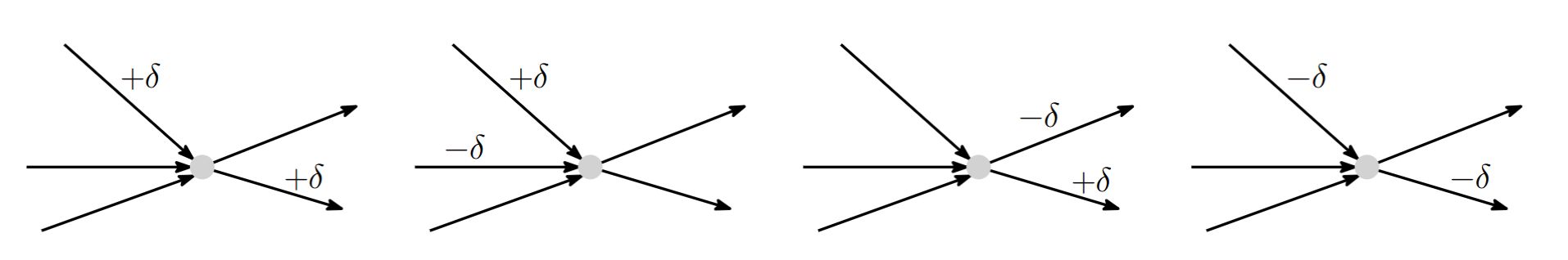
Die vier Typen entstehen aus den Kombinationen \((+\delta\text{ rein}, +\delta\text{ raus})\), \((+\delta\text{ rein}, -\delta\text{ rein})\), \((+\delta\text{ raus}, -\delta\text{ raus})\), \((-\delta\text{ raus}, -\delta\text{ rein})\).
Die Bilanz an jedem inneren Knoten bleibt unverändert.
Field-by-field Comparison
| Field |
Before |
After |
| Extra |
Die vier Typen entstehen aus den Kombinationen \((+\delta\text{ rein}, +\delta\text{ raus})\), \((-\delta\text{ rein}, +\delta\text{ raus})\), \((+\delta\text{ raus}, -\delta\text{ rein})\), \((-\delta\text{ raus}, -\delta\text{ rein})\). Die Bilanz an jedem inneren Knoten bleibt unverändert. |
<img src="paste-8143f132e2e57c20eaa88afb6a205d2866f761d8.jpg"><br><br>Die vier Typen entstehen aus den Kombinationen \((+\delta\text{ rein}, +\delta\text{ raus})\), \((+\delta\text{ rein}, -\delta\text{ rein})\), \((+\delta\text{ raus}, -\delta\text{ raus})\), \((-\delta\text{ raus}, -\delta\text{ rein})\). <br><br>Die Bilanz an jedem inneren Knoten bleibt unverändert. |
Tags:
ETH::2._Semester::A&W::3._Algorithmen_-_Highlights::1._Graphenalgorithmen::3._Minimale_Schnitte_in_Graphen
Note 3: ETH::2. Semester::A&W
Deck: ETH::2. Semester::A&W
Note Type: Horvath Cloze
GUID: KyltqkDci3
modified
Before
Front
ETH::2._Semester::A&W::3._Algorithmen_-_Highlights::1._Graphenalgorithmen::2._Flüsse_in_Netzwerken
Der Wert eines Flusses \(f\) ist definiert als der Nettoabfluss der Quelle:\[\operatorname{val}(f) := \operatorname{netoutflow}(s) := {{c2::\sum_{u \in V : (s,u) \in A} f(s, u) \;-\; \sum_{u \in V : (u,s) \in A} f(u, s)}}.\]
Back
ETH::2._Semester::A&W::3._Algorithmen_-_Highlights::1._Graphenalgorithmen::2._Flüsse_in_Netzwerken
Der Wert eines Flusses \(f\) ist definiert als der Nettoabfluss der Quelle:\[\operatorname{val}(f) := \operatorname{netoutflow}(s) := {{c2::\sum_{u \in V : (s,u) \in A} f(s, u) \;-\; \sum_{u \in V : (u,s) \in A} f(u, s)}}.\]
Eingehende Kanten an der Quelle werden abgezogen.
After
Front
ETH::2._Semester::A&W::3._Algorithmen_-_Highlights::1._Graphenalgorithmen::2._Flüsse_in_Netzwerken
Der Wert eines Flusses \(f\) ist definiert als der Nettoabfluss der Quelle:\[\operatorname{val}(f) := {{c1::\operatorname{netoutflow}(s) := \sum_{u \in V : (s,u) \in A} f(s, u) \;-\; \sum_{u \in V : (u,s) \in A} f(u, s). }}\]
Back
ETH::2._Semester::A&W::3._Algorithmen_-_Highlights::1._Graphenalgorithmen::2._Flüsse_in_Netzwerken
Der Wert eines Flusses \(f\) ist definiert als der Nettoabfluss der Quelle:\[\operatorname{val}(f) := {{c1::\operatorname{netoutflow}(s) := \sum_{u \in V : (s,u) \in A} f(s, u) \;-\; \sum_{u \in V : (u,s) \in A} f(u, s). }}\]
Eingehende Kanten an der Quelle werden abgezogen.
Field-by-field Comparison
| Field |
Before |
After |
| Text |
Der <b>Wert</b> eines Flusses \(f\) ist definiert als der {{c1::Nettoabfluss der Quelle}}:\[\operatorname{val}(f) := \operatorname{netoutflow}(s) := {{c2::\sum_{u \in V : (s,u) \in A} f(s, u) \;-\; \sum_{u \in V : (u,s) \in A} f(u, s)}}.\] |
Der <b>Wert</b> eines Flusses \(f\) ist definiert als {{c1::der Nettoabfluss der Quelle}}:\[\operatorname{val}(f) := {{c1::\operatorname{netoutflow}(s) := \sum_{u \in V : (s,u) \in A} f(s, u) \;-\; \sum_{u \in V : (u,s) \in A} f(u, s). }}\] |
Tags:
ETH::2._Semester::A&W::3._Algorithmen_-_Highlights::1._Graphenalgorithmen::2._Flüsse_in_Netzwerken
Note 4: ETH::2. Semester::A&W
Deck: ETH::2. Semester::A&W
Note Type: Horvath Cloze
GUID: L%pGeRiAOW
modified
Before
Front
ETH::2._Semester::A&W::3._Algorithmen_-_Highlights::1._Graphenalgorithmen::2._Flüsse_in_Netzwerken
MaxFlow-Problem. Gegeben ein Netzwerk \(N = (V, A, c, s, t)\), finde einen Fluss \(f\) grössten Werts (einen maximalen Fluss).
Back
ETH::2._Semester::A&W::3._Algorithmen_-_Highlights::1._Graphenalgorithmen::2._Flüsse_in_Netzwerken
MaxFlow-Problem. Gegeben ein Netzwerk \(N = (V, A, c, s, t)\), finde einen Fluss \(f\) grössten Werts (einen maximalen Fluss).
Der Wert eines Flusses wird über den Nettoabfluss der Quelle gemessen.
After
Front
ETH::2._Semester::A&W::3._Algorithmen_-_Highlights::1._Graphenalgorithmen::2._Flüsse_in_Netzwerken
MaxFlow-Problem
Gegeben ein Netzwerk \(N = (V, A, c, s, t)\), finde einen Fluss \(f\) grössten Werts (einen maximalen Fluss).
Back
ETH::2._Semester::A&W::3._Algorithmen_-_Highlights::1._Graphenalgorithmen::2._Flüsse_in_Netzwerken
MaxFlow-Problem
Gegeben ein Netzwerk \(N = (V, A, c, s, t)\), finde einen Fluss \(f\) grössten Werts (einen maximalen Fluss).
Der Wert eines Flusses wird über den Nettoabfluss der Quelle gemessen.
Field-by-field Comparison
| Field |
Before |
After |
| Text |
<b>MaxFlow-Problem.</b> Gegeben ein {{c1::Netzwerk \(N = (V, A, c, s, t)\)}}, finde einen {{c2::Fluss \(f\) grössten Werts (einen <i>maximalen</i> Fluss)}}. |
<b>MaxFlow-Problem</b><br>Gegeben ein {{c1::Netzwerk \(N = (V, A, c, s, t)\)}}, finde einen {{c2::Fluss \(f\) grössten Werts (einen <i>maximalen</i> Fluss)}}. |
Tags:
ETH::2._Semester::A&W::3._Algorithmen_-_Highlights::1._Graphenalgorithmen::2._Flüsse_in_Netzwerken
Note 5: ETH::2. Semester::A&W
Deck: ETH::2. Semester::A&W
Note Type: Horvath Cloze
GUID: Vixq;:@kAb
modified
Before
Front
ETH::2._Semester::A&W::3._Algorithmen_-_Highlights::1._Graphenalgorithmen::3._Minimale_Schnitte_in_Graphen
Da es nur
endlich viele s-t-Schnitte gibt, folgt:
- s-t-MinCut ist ein endliches algorithmisches Problem,
- ein minimaler Schnitt existiert immer.
Back
ETH::2._Semester::A&W::3._Algorithmen_-_Highlights::1._Graphenalgorithmen::3._Minimale_Schnitte_in_Graphen
Da es nur
endlich viele s-t-Schnitte gibt, folgt:
- s-t-MinCut ist ein endliches algorithmisches Problem,
- ein minimaler Schnitt existiert immer.
Im Gegensatz dazu ist die Menge der zulässigen Flüsse im Allgemeinen unendlich (reelle Kapazitäten), aber das Supremum wird ebenfalls angenommen (Maxflow-Mincut).
After
Front
ETH::2._Semester::A&W::3._Algorithmen_-_Highlights::1._Graphenalgorithmen::3._Minimale_Schnitte_in_Graphen
Da es
nur endlich viele s-t-Schnitte gibt, folgt:
- s-t-MinCut ist ein endliches algorithmisches Problem,
- ein minimaler Schnitt existiert immer.
Back
ETH::2._Semester::A&W::3._Algorithmen_-_Highlights::1._Graphenalgorithmen::3._Minimale_Schnitte_in_Graphen
Da es
nur endlich viele s-t-Schnitte gibt, folgt:
- s-t-MinCut ist ein endliches algorithmisches Problem,
- ein minimaler Schnitt existiert immer.
Im Gegensatz dazu ist die Menge der zulässigen Flüsse im Allgemeinen unendlich (reelle Kapazitäten), aber das Supremum wird ebenfalls angenommen (Maxflow-Mincut).
Field-by-field Comparison
| Field |
Before |
After |
| Text |
Da es nur {{c1::endlich viele s-t-Schnitte}} gibt, folgt:<ul><li>s-t-MinCut ist {{c2::ein endliches algorithmisches Problem}},</li><li>{{c3::ein minimaler Schnitt existiert immer}}.</li></ul> |
Da es {{c1::nur endlich viele s-t-Schnitte}} gibt, folgt:<ul><li>s-t-MinCut ist {{c2::ein endliches algorithmisches Problem}},</li><li>{{c3::ein minimaler Schnitt existiert immer}}.</li></ul> |
Tags:
ETH::2._Semester::A&W::3._Algorithmen_-_Highlights::1._Graphenalgorithmen::3._Minimale_Schnitte_in_Graphen
Note 6: ETH::2. Semester::A&W
Deck: ETH::2. Semester::A&W
Note Type: Horvath Cloze
GUID: XE[{x!N{Fm
modified
Before
Front
ETH::2._Semester::A&W::3._Algorithmen_-_Highlights::1._Graphenalgorithmen::1._Lange_Pfade
Satz (Zufallsfärbungen)Sei \(G\) ein Graph mit einem Pfad \(P\) der Länge \(k-1\).
- Eine zufällige Färbung mit \(k\) Farben erzeugt einen bunten Pfad der Länge \(k-1\) mit Wahrscheinlichkeit \(p \geq {{c1::e^{-k} }}\).
- Bei wiederholten Färbungen mit \(k\) Farben ist der Erwartungswert der Anzahl der Versuche, bis man einen bunten Pfad der Länge \(k-1\) erhält, \(\tfrac{1}{p} \leq {{c2::e^{k} }}\).
Back
ETH::2._Semester::A&W::3._Algorithmen_-_Highlights::1._Graphenalgorithmen::1._Lange_Pfade
Satz (Zufallsfärbungen)Sei \(G\) ein Graph mit einem Pfad \(P\) der Länge \(k-1\).
- Eine zufällige Färbung mit \(k\) Farben erzeugt einen bunten Pfad der Länge \(k-1\) mit Wahrscheinlichkeit \(p \geq {{c1::e^{-k} }}\).
- Bei wiederholten Färbungen mit \(k\) Farben ist der Erwartungswert der Anzahl der Versuche, bis man einen bunten Pfad der Länge \(k-1\) erhält, \(\tfrac{1}{p} \leq {{c2::e^{k} }}\).
Beweis von (1): \(\Pr[P \text{ wird bunt}] = \tfrac{k!}{k^k} \geq e^{-k}\) per Stirling.
Beweis von (2): geometrisch verteilte Wartezeit mit Erfolgswahrscheinlichkeit \(p\), Erwartungswert \(1/p\).
After
Front
ETH::2._Semester::A&W::3._Algorithmen_-_Highlights::1._Graphenalgorithmen::1._Lange_Pfade
ZufallsfärbungenSei \(G\) ein Graph mit einem Pfad \(P\) der Länge \(k-1\).
- Eine zufällige Färbung mit \(k\) Farben erzeugt einen bunten Pfad der Länge \(k-1\) mit Wahrscheinlichkeit \(p \geq {{c1::e^{-k} }}\).
- Bei wiederholten Färbungen mit \(k\) Farben ist der Erwartungswert der Anzahl der Versuche, bis man einen bunten Pfad der Länge \(k-1\) erhält, \(\tfrac{1}{p} \leq {{c2::e^{k} }}\).
Back
ETH::2._Semester::A&W::3._Algorithmen_-_Highlights::1._Graphenalgorithmen::1._Lange_Pfade
ZufallsfärbungenSei \(G\) ein Graph mit einem Pfad \(P\) der Länge \(k-1\).
- Eine zufällige Färbung mit \(k\) Farben erzeugt einen bunten Pfad der Länge \(k-1\) mit Wahrscheinlichkeit \(p \geq {{c1::e^{-k} }}\).
- Bei wiederholten Färbungen mit \(k\) Farben ist der Erwartungswert der Anzahl der Versuche, bis man einen bunten Pfad der Länge \(k-1\) erhält, \(\tfrac{1}{p} \leq {{c2::e^{k} }}\).
Beweis von (1): \(\Pr[P \text{ wird bunt}] = \tfrac{k!}{k^k} \geq e^{-k}\) per Stirling.
Beweis von (2): geometrisch verteilte Wartezeit mit Erfolgswahrscheinlichkeit \(p\), Erwartungswert \(1/p\).
Field-by-field Comparison
| Field |
Before |
After |
| Text |
<b>Satz (Zufallsfärbungen)</b><br>Sei \(G\) ein Graph mit einem Pfad \(P\) der Länge \(k-1\).<br><ol><li>Eine zufällige Färbung mit \(k\) Farben erzeugt einen bunten Pfad der Länge \(k-1\) mit Wahrscheinlichkeit \(p \geq {{c1::e^{-k} }}\).</li><li>Bei wiederholten Färbungen mit \(k\) Farben ist der Erwartungswert der Anzahl der Versuche, bis man einen bunten Pfad der Länge \(k-1\) erhält, \(\tfrac{1}{p} \leq {{c2::e^{k} }}\).</li></ol> |
<b>Zufallsfärbungen</b><br>Sei \(G\) ein Graph mit einem Pfad \(P\) der Länge \(k-1\).<br><ol><li>Eine zufällige Färbung mit \(k\) Farben erzeugt einen bunten Pfad der Länge \(k-1\) mit Wahrscheinlichkeit \(p \geq {{c1::e^{-k} }}\).</li><li>Bei wiederholten Färbungen mit \(k\) Farben ist der Erwartungswert der Anzahl der Versuche, bis man einen bunten Pfad der Länge \(k-1\) erhält, \(\tfrac{1}{p} \leq {{c2::e^{k} }}\).</li></ol> |
Tags:
ETH::2._Semester::A&W::3._Algorithmen_-_Highlights::1._Graphenalgorithmen::1._Lange_Pfade
Note 7: ETH::2. Semester::A&W
Deck: ETH::2. Semester::A&W
Note Type: Horvath Cloze
GUID: Y!-po8YFmj
modified
Before
Front
ETH::2._Semester::A&W::3._Algorithmen_-_Highlights::1._Graphenalgorithmen::2._Flüsse_in_Netzwerken
Lemma (Nettozufluss der Senke). Für jeden Fluss \(f\) gilt: der Nettozufluss der Senke gleicht dem Wert des Flusses:\[\operatorname{netinflow}(t) := \sum_{u \in V : (u,t) \in A} f(u, t) \;-\; \sum_{u \in V : (t,u) \in A} f(t, u) \;=\; {{c2::\operatorname{val}(f)}}.\]
Back
ETH::2._Semester::A&W::3._Algorithmen_-_Highlights::1._Graphenalgorithmen::2._Flüsse_in_Netzwerken
Lemma (Nettozufluss der Senke). Für jeden Fluss \(f\) gilt: der Nettozufluss der Senke gleicht dem Wert des Flusses:\[\operatorname{netinflow}(t) := \sum_{u \in V : (u,t) \in A} f(u, t) \;-\; \sum_{u \in V : (t,u) \in A} f(t, u) \;=\; {{c2::\operatorname{val}(f)}}.\]
Intuition: Was bei der Quelle herausfliesst, muss bei der Senke ankommen. Beweis via Flusserhaltung an den inneren Knoten und Aufsummieren über alle \(v \in V \setminus \{s\}\). Proof Included
After
Front
ETH::2._Semester::A&W::3._Algorithmen_-_Highlights::1._Graphenalgorithmen::2._Flüsse_in_Netzwerken
Für jeden Fluss \(f\) gilt: der Nettozufluss der Senke gleicht dem Wert des Flusses:\[\operatorname{netinflow}(t) := \sum_{u \in V : (u,t) \in A} f(u, t) \;-\; \sum_{u \in V : (t,u) \in A} f(t, u) \;=\; {{c1::\operatorname{val}(f)}}.\]
Back
ETH::2._Semester::A&W::3._Algorithmen_-_Highlights::1._Graphenalgorithmen::2._Flüsse_in_Netzwerken
Für jeden Fluss \(f\) gilt: der Nettozufluss der Senke gleicht dem Wert des Flusses:\[\operatorname{netinflow}(t) := \sum_{u \in V : (u,t) \in A} f(u, t) \;-\; \sum_{u \in V : (t,u) \in A} f(t, u) \;=\; {{c1::\operatorname{val}(f)}}.\]
Intuition: Was bei der Quelle herausfliesst, muss bei der Senke ankommen. Beweis via Flusserhaltung an den inneren Knoten und Aufsummieren über alle \(v \in V \setminus \{s\}\).
Field-by-field Comparison
| Field |
Before |
After |
| Text |
<b>Lemma (Nettozufluss der Senke).</b> Für jeden Fluss \(f\) gilt: der Nettozufluss der Senke gleicht {{c1::dem Wert des Flusses}}:\[\operatorname{netinflow}(t) := \sum_{u \in V : (u,t) \in A} f(u, t) \;-\; \sum_{u \in V : (t,u) \in A} f(t, u) \;=\; {{c2::\operatorname{val}(f)}}.\] |
Für jeden Fluss \(f\) gilt: der Nettozufluss der Senke gleicht {{c1::dem Wert des Flusses}}:\[\operatorname{netinflow}(t) := \sum_{u \in V : (u,t) \in A} f(u, t) \;-\; \sum_{u \in V : (t,u) \in A} f(t, u) \;=\; {{c1::\operatorname{val}(f)}}.\] |
| Extra |
Intuition: Was bei der Quelle herausfliesst, muss bei der Senke ankommen. Beweis via Flusserhaltung an den inneren Knoten und Aufsummieren über alle \(v \in V \setminus \{s\}\). <i>Proof Included</i> |
Intuition: Was bei der Quelle herausfliesst, muss bei der Senke ankommen. Beweis via Flusserhaltung an den inneren Knoten und Aufsummieren über alle \(v \in V \setminus \{s\}\). |
Tags:
ETH::2._Semester::A&W::3._Algorithmen_-_Highlights::1._Graphenalgorithmen::2._Flüsse_in_Netzwerken
Note 8: ETH::2. Semester::A&W
Deck: ETH::2. Semester::A&W
Note Type: Horvath Cloze
GUID: [I%rT#:,Sz
modified
Before
Front
ETH::2._Semester::A&W::3._Algorithmen_-_Highlights::1._Graphenalgorithmen::3._Minimale_Schnitte_in_Graphen
Notation. Für eine Kante \(e = (u, v)\) sei \(e^{\mathrm{opp}} := (v, u)\). Im Spielraum einer Kante mit Kapazität \(c\) und Fluss \(f\) haben wir vorwärts den Vorrat \(c - f\) und rückwärts den Vorrat \(f\).
Back
ETH::2._Semester::A&W::3._Algorithmen_-_Highlights::1._Graphenalgorithmen::3._Minimale_Schnitte_in_Graphen
Notation. Für eine Kante \(e = (u, v)\) sei \(e^{\mathrm{opp}} := (v, u)\). Im Spielraum einer Kante mit Kapazität \(c\) und Fluss \(f\) haben wir vorwärts den Vorrat \(c - f\) und rückwärts den Vorrat \(f\).
Vorwärts: noch \(c - f\) zusätzliche Einheiten möglich. Rückwärts: bis zu \(f\) Einheiten lassen sich „zurückgeben“. Diese beiden Werte werden im Restnetzwerk zu zwei separaten Kanten.
After
Front
ETH::2._Semester::A&W::3._Algorithmen_-_Highlights::1._Graphenalgorithmen::3._Minimale_Schnitte_in_Graphen
Für eine Kante \(e = (u, v)\) sei \(e^{\mathrm{opp}} := (v, u)\).
Im Spielraum einer Kante mit Kapazität \(c\) und Fluss \(f\) haben wir vorwärts die Restkapazität \(c - f\) und rückwärts die Restkapazität \(f\).
Back
ETH::2._Semester::A&W::3._Algorithmen_-_Highlights::1._Graphenalgorithmen::3._Minimale_Schnitte_in_Graphen
Für eine Kante \(e = (u, v)\) sei \(e^{\mathrm{opp}} := (v, u)\).
Im Spielraum einer Kante mit Kapazität \(c\) und Fluss \(f\) haben wir vorwärts die Restkapazität \(c - f\) und rückwärts die Restkapazität \(f\).
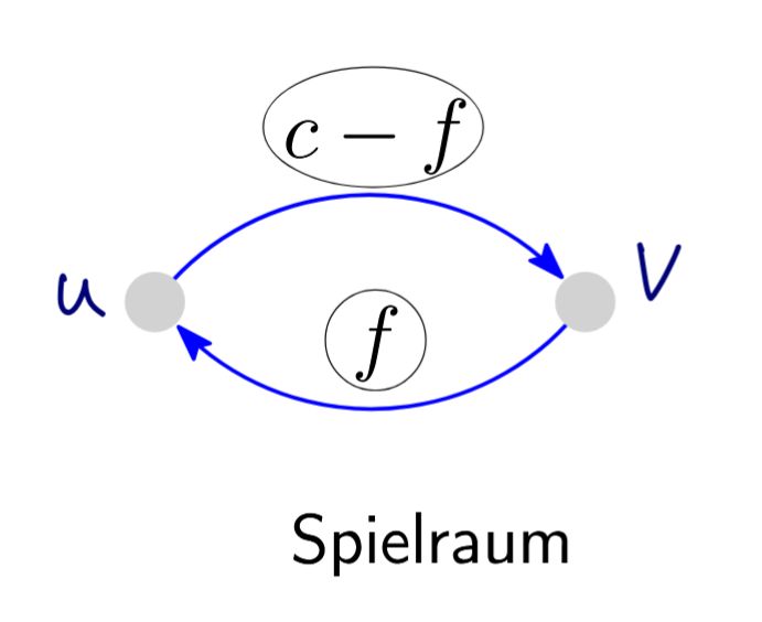
Vorwärts: noch \(c - f\) zusätzliche Einheiten möglich. Rückwärts: bis zu \(f\) Einheiten lassen sich „zurückgeben“. Diese beiden Werte werden im Restnetzwerk zu zwei separaten Kanten.
Field-by-field Comparison
| Field |
Before |
After |
| Text |
<b>Notation.</b> Für eine Kante \(e = (u, v)\) sei \(e^{\mathrm{opp}} := {{c1::(v, u)}}\). Im <b>Spielraum</b> einer Kante mit Kapazität \(c\) und Fluss \(f\) haben wir vorwärts den Vorrat \({{c2::c - f}}\) und rückwärts den Vorrat \({{c3::f}}\). |
Für eine Kante \(e = (u, v)\) sei \(e^{\mathrm{opp}} := {{c1::(v, u)}}\). <br><br>Im <b>Spielraum</b> einer Kante mit Kapazität \(c\) und Fluss \(f\) haben wir vorwärts die Restkapazität \({{c2::c - f}}\) und rückwärts die Restkapazität \({{c2::f}}\). |
| Extra |
Vorwärts: noch \(c - f\) zusätzliche Einheiten möglich. Rückwärts: bis zu \(f\) Einheiten lassen sich „zurückgeben“. Diese beiden Werte werden im Restnetzwerk zu zwei separaten Kanten. |
<img src="paste-c831d6bdcdb2a0fcbcd996592269907f651f1512.jpg"><br><br>Vorwärts: noch \(c - f\) zusätzliche Einheiten möglich. Rückwärts: bis zu \(f\) Einheiten lassen sich „zurückgeben“. Diese beiden Werte werden im Restnetzwerk zu zwei separaten Kanten. |
Tags:
ETH::2._Semester::A&W::3._Algorithmen_-_Highlights::1._Graphenalgorithmen::3._Minimale_Schnitte_in_Graphen
Note 9: ETH::2. Semester::A&W
Deck: ETH::2. Semester::A&W
Note Type: Horvath Cloze
GUID: a(.3t3[#-=
modified
Before
Front
ETH::2._Semester::A&W::3._Algorithmen_-_Highlights::1._Graphenalgorithmen::2._Flüsse_in_Netzwerken
Sei \(N = (V, A, c, s, t)\) ein Netzwerk. Ein
Fluss in \(N\) ist eine Funktion \(f : A \to \mathbb{R}\) mit:
- Zulässigkeit: \[{{c2::0 \leq f(e) \leq c(e) \quad \text{für alle } e \in A}}\]
- Flusserhaltung: für alle \(v \in V \setminus \{s, t\}\) gilt \[{{c4::\sum_{u \in V : (u,v) \in A} f(u, v) \;=\; \sum_{u \in V : (v,u) \in A} f(v, u)}}\]
Back
ETH::2._Semester::A&W::3._Algorithmen_-_Highlights::1._Graphenalgorithmen::2._Flüsse_in_Netzwerken
Sei \(N = (V, A, c, s, t)\) ein Netzwerk. Ein
Fluss in \(N\) ist eine Funktion \(f : A \to \mathbb{R}\) mit:
- Zulässigkeit: \[{{c2::0 \leq f(e) \leq c(e) \quad \text{für alle } e \in A}}\]
- Flusserhaltung: für alle \(v \in V \setminus \{s, t\}\) gilt \[{{c4::\sum_{u \in V : (u,v) \in A} f(u, v) \;=\; \sum_{u \in V : (v,u) \in A} f(v, u)}}\]
Flusserhaltung gilt nur an inneren Knoten, nicht an Quelle oder Senke. Anschaulich: was hineinfliesst, fliesst auch hinaus.
After
Front
ETH::2._Semester::A&W::3._Algorithmen_-_Highlights::1._Graphenalgorithmen::2._Flüsse_in_Netzwerken
Sei \(N = (V, A, c, s, t)\) ein Netzwerk. Ein
Fluss in \(N\) ist eine Funktion \(f : A \to \mathbb{R}\) mit:
- {{c1::Zulässigkeit: \[0 \leq f(e) \leq c(e) \quad \text{für alle } e \in A\]}}
- {{c2::Flusserhaltung: für alle \(v \in V \setminus \{s, t\}\) gilt \[\sum_{u \in V : (u,v) \in A} f(u, v) \;=\; \sum_{u \in V : (v,u) \in A} f(v, u)\]}}
Back
ETH::2._Semester::A&W::3._Algorithmen_-_Highlights::1._Graphenalgorithmen::2._Flüsse_in_Netzwerken
Sei \(N = (V, A, c, s, t)\) ein Netzwerk. Ein
Fluss in \(N\) ist eine Funktion \(f : A \to \mathbb{R}\) mit:
- {{c1::Zulässigkeit: \[0 \leq f(e) \leq c(e) \quad \text{für alle } e \in A\]}}
- {{c2::Flusserhaltung: für alle \(v \in V \setminus \{s, t\}\) gilt \[\sum_{u \in V : (u,v) \in A} f(u, v) \;=\; \sum_{u \in V : (v,u) \in A} f(v, u)\]}}
Flusserhaltung gilt nur an inneren Knoten, nicht an Quelle oder Senke. Anschaulich: was hineinfliesst, fliesst auch hinaus.
Field-by-field Comparison
| Field |
Before |
After |
| Text |
Sei \(N = (V, A, c, s, t)\) ein Netzwerk. Ein <b>Fluss</b> in \(N\) ist eine Funktion \(f : A \to \mathbb{R}\) mit:<ul><li>{{c1::<b>Zulässigkeit</b>}}: \[{{c2::0 \leq f(e) \leq c(e) \quad \text{für alle } e \in A}}\]</li><li>{{c3::<b>Flusserhaltung</b>}}: für alle \(v \in V \setminus \{s, t\}\) gilt \[{{c4::\sum_{u \in V : (u,v) \in A} f(u, v) \;=\; \sum_{u \in V : (v,u) \in A} f(v, u)}}\]</li></ul> |
Sei \(N = (V, A, c, s, t)\) ein Netzwerk. Ein <b>Fluss</b> in \(N\) ist eine Funktion \(f : A \to \mathbb{R}\) mit:<br><ol><li>{{c1::<b>Zulässigkeit</b>: \[0 \leq f(e) \leq c(e) \quad \text{für alle } e \in A\]}}</li><li>{{c2::<b>Flusserhaltung</b>: für alle \(v \in V \setminus \{s, t\}\) gilt \[\sum_{u \in V : (u,v) \in A} f(u, v) \;=\; \sum_{u \in V : (v,u) \in A} f(v, u)\]}}</li></ol> |
Tags:
ETH::2._Semester::A&W::3._Algorithmen_-_Highlights::1._Graphenalgorithmen::2._Flüsse_in_Netzwerken
Note 10: ETH::2. Semester::A&W
Deck: ETH::2. Semester::A&W
Note Type: Horvath Classic
GUID: itUq/f`To4
modified
Before
Front
ETH::2._Semester::A&W::1._Graphentheorie::7._Färbungen ETH::2._Semester::A&W::Minitests::2
Wahr oder falsch?
Ist \(G\) ein Graph mit maximalem Grad \(\Delta(G)\), so findet der Greedy-Algorithmus (mit beliebiger Knotenreihenfolge) stets eine zulässige Färbung mit höchstens \(\Delta(G) + 1\) Farben.
Back
ETH::2._Semester::A&W::1._Graphentheorie::7._Färbungen ETH::2._Semester::A&W::Minitests::2
Wahr oder falsch?
Ist \(G\) ein Graph mit maximalem Grad \(\Delta(G)\), so findet der Greedy-Algorithmus (mit beliebiger Knotenreihenfolge) stets eine zulässige Färbung mit höchstens \(\Delta(G) + 1\) Farben.
Wahr
After
Front
ETH::2._Semester::A&W::1._Graphentheorie::7._Färbungen ETH::2._Semester::A&W::Minitests::2
Wahr oder falsch?
Ist \(G\) ein Graph mit maximalem Grad \(\Delta(G)\), so findet der Greedy-Algorithmus (mit beliebiger Knotenreihenfolge) stets eine zulässige Färbung mit höchstens \(\Delta(G) + 1\) Farben.
Back
ETH::2._Semester::A&W::1._Graphentheorie::7._Färbungen ETH::2._Semester::A&W::Minitests::2
Wahr oder falsch?
Ist \(G\) ein Graph mit maximalem Grad \(\Delta(G)\), so findet der Greedy-Algorithmus (mit beliebiger Knotenreihenfolge) stets eine zulässige Färbung mit höchstens \(\Delta(G) + 1\) Farben.
Wahr.
Field-by-field Comparison
| Field |
Before |
After |
| Back |
Wahr |
Wahr. |
Tags:
ETH::2._Semester::A&W::1._Graphentheorie::7._Färbungen
ETH::2._Semester::A&W::Minitests::2
Note 11: ETH::2. Semester::A&W
Deck: ETH::2. Semester::A&W
Note Type: Horvath Cloze
GUID: lg(2GdY~w`
modified
Before
Front
ETH::2._Semester::A&W::3._Algorithmen_-_Highlights::1._Graphenalgorithmen::2._Flüsse_in_Netzwerken
Lemma (schwache Dualität). Ist \(f\) ein Fluss und \((S, T)\) ein s-t-Schnitt in einem Netzwerk, so gilt\[{{c1::\operatorname{val}(f) \;\leq\; \operatorname{cap}(S, T)}}.\]
Back
ETH::2._Semester::A&W::3._Algorithmen_-_Highlights::1._Graphenalgorithmen::2._Flüsse_in_Netzwerken
Lemma (schwache Dualität). Ist \(f\) ein Fluss und \((S, T)\) ein s-t-Schnitt in einem Netzwerk, so gilt\[{{c1::\operatorname{val}(f) \;\leq\; \operatorname{cap}(S, T)}}.\]
Konsequenz: Findet man zu einem Fluss \(f\) einen Schnitt \((S, T)\) mit \(\operatorname{val}(f) = \operatorname{cap}(S, T)\), so ist \(f\) maximal. Der Schnitt ist dann ein einfaches Zertifikat für die Maximalität.
After
Front
ETH::2._Semester::A&W::3._Algorithmen_-_Highlights::1._Graphenalgorithmen::2._Flüsse_in_Netzwerken
Schwache Dualität
Ist \(f\) ein Fluss und \((S, T)\) ein s-t-Schnitt in einem Netzwerk, so gilt\[{{c1::\operatorname{val}(f) \;\leq\; \operatorname{cap}(S, T)}}.\]
Back
ETH::2._Semester::A&W::3._Algorithmen_-_Highlights::1._Graphenalgorithmen::2._Flüsse_in_Netzwerken
Schwache Dualität
Ist \(f\) ein Fluss und \((S, T)\) ein s-t-Schnitt in einem Netzwerk, so gilt\[{{c1::\operatorname{val}(f) \;\leq\; \operatorname{cap}(S, T)}}.\]
Konsequenz: Findet man zu einem Fluss \(f\) einen Schnitt \((S, T)\) mit \(\operatorname{val}(f) = \operatorname{cap}(S, T)\), so ist \(f\) maximal. Der Schnitt ist dann ein einfaches Zertifikat für die Maximalität.
Field-by-field Comparison
| Field |
Before |
After |
| Text |
<b>Lemma (schwache Dualität).</b> Ist \(f\) ein Fluss und \((S, T)\) ein s-t-Schnitt in einem Netzwerk, so gilt\[{{c1::\operatorname{val}(f) \;\leq\; \operatorname{cap}(S, T)}}.\] |
<b>Schwache Dualität</b><br>Ist \(f\) ein Fluss und \((S, T)\) ein s-t-Schnitt in einem Netzwerk, so gilt\[{{c1::\operatorname{val}(f) \;\leq\; \operatorname{cap}(S, T)}}.\] |
Tags:
ETH::2._Semester::A&W::3._Algorithmen_-_Highlights::1._Graphenalgorithmen::2._Flüsse_in_Netzwerken
Note 12: ETH::2. Semester::A&W
Deck: ETH::2. Semester::A&W
Note Type: Horvath Classic
GUID: s!zsm$&sf}
modified
Before
Front
ETH::2._Semester::A&W::1._Graphentheorie::6._Matchings ETH::2._Semester::A&W::Minitests::2
Wahr oder falsch?
Für einen vollständigen Graphen \(G\) mit gerader Anzahl von Knoten und positiven Gewichten \(\ell(x,y)\), der die Dreiecksungleichung erfüllt, sei \(M\) ein perfektes Matching mit minimalen Kosten und \(C\) die minimale Kosten-Reise des Handlungsreisenden (TSP-Tour). Dann ist \(\ell(M) \leq \ell(C)/2\).
Back
ETH::2._Semester::A&W::1._Graphentheorie::6._Matchings ETH::2._Semester::A&W::Minitests::2
Wahr oder falsch?
Für einen vollständigen Graphen \(G\) mit gerader Anzahl von Knoten und positiven Gewichten \(\ell(x,y)\), der die Dreiecksungleichung erfüllt, sei \(M\) ein perfektes Matching mit minimalen Kosten und \(C\) die minimale Kosten-Reise des Handlungsreisenden (TSP-Tour). Dann ist \(\ell(M) \leq \ell(C)/2\).
Wahr
After
Front
ETH::2._Semester::A&W::1._Graphentheorie::6._Matchings ETH::2._Semester::A&W::Minitests::2
Wahr oder falsch?
Für einen vollständigen Graphen \(G\) mit gerader Anzahl von Knoten und positiven Gewichten \(\ell(x,y)\), der die Dreiecksungleichung erfüllt, sei \(M\) ein perfektes Matching mit minimalen Kosten und \(C\) die minimale Kosten-Reise des Handlungsreisenden (TSP-Tour).
Dann ist \(\ell(M) \leq \ell(C)/2\).
Back
ETH::2._Semester::A&W::1._Graphentheorie::6._Matchings ETH::2._Semester::A&W::Minitests::2
Wahr oder falsch?
Für einen vollständigen Graphen \(G\) mit gerader Anzahl von Knoten und positiven Gewichten \(\ell(x,y)\), der die Dreiecksungleichung erfüllt, sei \(M\) ein perfektes Matching mit minimalen Kosten und \(C\) die minimale Kosten-Reise des Handlungsreisenden (TSP-Tour).
Dann ist \(\ell(M) \leq \ell(C)/2\).
Wahr.
Field-by-field Comparison
| Field |
Before |
After |
| Front |
Wahr oder falsch?<br><br>Für einen vollständigen Graphen \(G\) mit gerader Anzahl von Knoten und positiven Gewichten \(\ell(x,y)\), der die Dreiecksungleichung erfüllt, sei \(M\) ein perfektes Matching mit minimalen Kosten und \(C\) die minimale Kosten-Reise des Handlungsreisenden (TSP-Tour). Dann ist \(\ell(M) \leq \ell(C)/2\). |
Wahr oder falsch?<br><br>Für einen vollständigen Graphen \(G\) mit gerader Anzahl von Knoten und positiven Gewichten \(\ell(x,y)\), der die Dreiecksungleichung erfüllt, sei \(M\) ein perfektes Matching mit minimalen Kosten und \(C\) die minimale Kosten-Reise des Handlungsreisenden (TSP-Tour). <br><br>Dann ist \(\ell(M) \leq \ell(C)/2\). |
| Back |
Wahr |
Wahr. |
Tags:
ETH::2._Semester::A&W::1._Graphentheorie::6._Matchings
ETH::2._Semester::A&W::Minitests::2
Note 13: ETH::2. Semester::A&W
Deck: ETH::2. Semester::A&W
Note Type: Horvath Cloze
GUID: vi;%r.~JIf
modified
Before
Front
ETH::2._Semester::A&W::3._Algorithmen_-_Highlights::1._Graphenalgorithmen::3._Minimale_Schnitte_in_Graphen
Eine Flussaugmentierung ist eine Folge von lokalen Veränderungen entlang eines s-t-Pfads, bei dem auf jeder Kante entweder \(+\delta\) (in Vorwärtsrichtung) oder \(-\delta\) (in Rückwärtsrichtung) addiert wird. Da an Quelle und Senke keine Flusserhaltung gefordert ist, erhöht sich \(\operatorname{val}(f)\) genau um \(\delta\).
Back
ETH::2._Semester::A&W::3._Algorithmen_-_Highlights::1._Graphenalgorithmen::3._Minimale_Schnitte_in_Graphen
Eine Flussaugmentierung ist eine Folge von lokalen Veränderungen entlang eines s-t-Pfads, bei dem auf jeder Kante entweder \(+\delta\) (in Vorwärtsrichtung) oder \(-\delta\) (in Rückwärtsrichtung) addiert wird. Da an Quelle und Senke keine Flusserhaltung gefordert ist, erhöht sich \(\operatorname{val}(f)\) genau um \(\delta\).
Beachte: Augmentierende Pfade aus dem Matching-Kapitel sind ein verwandtes, aber anderes Konzept (alternierende Kanten in/aus \(M\)). Hier geht es um Restkapazitäten in einem Netzwerk.
After
Front
ETH::2._Semester::A&W::3._Algorithmen_-_Highlights::1._Graphenalgorithmen::3._Minimale_Schnitte_in_Graphen
Eine Flussaugmentierung ist eine Folge von lokalen Veränderungen entlang eines s-t-Pfads, bei dem auf jeder Kante entweder \(+\delta\) (in Vorwärtsrichtung) oder \(-\delta\) (in Rückwärtsrichtung) addiert wird.
Da an Quelle und Senke keine Flusserhaltung gefordert ist, erhöht sich \(\operatorname{val}(f)\) genau um \(\delta\).
Back
ETH::2._Semester::A&W::3._Algorithmen_-_Highlights::1._Graphenalgorithmen::3._Minimale_Schnitte_in_Graphen
Eine Flussaugmentierung ist eine Folge von lokalen Veränderungen entlang eines s-t-Pfads, bei dem auf jeder Kante entweder \(+\delta\) (in Vorwärtsrichtung) oder \(-\delta\) (in Rückwärtsrichtung) addiert wird.
Da an Quelle und Senke keine Flusserhaltung gefordert ist, erhöht sich \(\operatorname{val}(f)\) genau um \(\delta\).
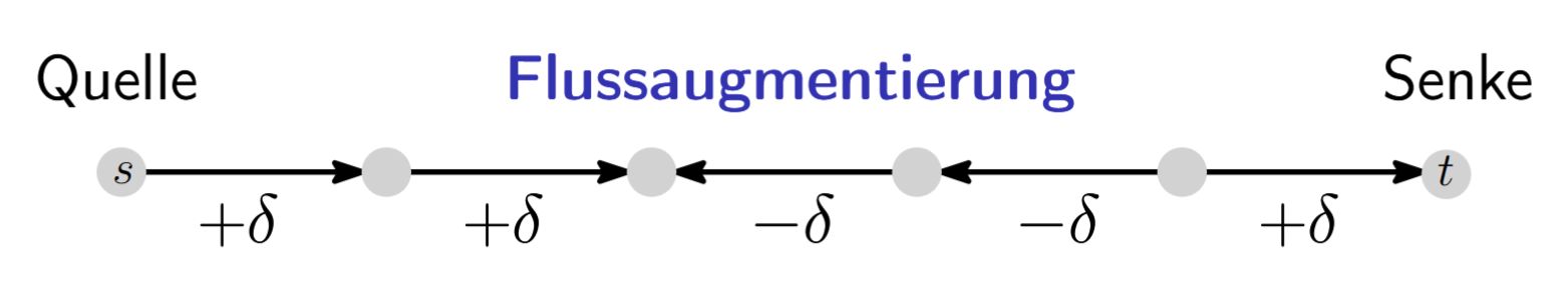
Beachte: Augmentierende Pfade aus dem Matching-Kapitel sind ein verwandtes, aber anderes Konzept (alternierende Kanten in/aus \(M\)). Hier geht es um Restkapazitäten in einem Netzwerk.
Field-by-field Comparison
| Field |
Before |
After |
| Text |
Eine <b>Flussaugmentierung</b> ist eine Folge von lokalen Veränderungen entlang eines s-t-Pfads, bei dem auf jeder Kante entweder \(+\delta\) (in Vorwärtsrichtung) oder \(-\delta\) (in Rückwärtsrichtung) addiert wird. Da {{c1::an Quelle und Senke keine Flusserhaltung gefordert ist}}, erhöht sich \(\operatorname{val}(f)\) genau um {{c2::\(\delta\)}}. |
Eine <b>Flussaugmentierung</b> ist eine Folge von lokalen Veränderungen entlang eines s-t-Pfads, bei dem auf jeder Kante entweder \(+\delta\) (in Vorwärtsrichtung) oder \(-\delta\) (in Rückwärtsrichtung) addiert wird. <br><br>Da {{c1::an Quelle und Senke keine Flusserhaltung gefordert ist}}, erhöht sich \(\operatorname{val}(f)\) genau um \(\delta\). |
| Extra |
<b>Beachte:</b> Augmentierende Pfade aus dem Matching-Kapitel sind ein verwandtes, aber anderes Konzept (alternierende Kanten in/aus \(M\)). Hier geht es um Restkapazitäten in einem Netzwerk. |
<img src="paste-85cc79947c499df1757e8d9f0cdbe5ec19f455b1.jpg"><b><br><br>Beachte:</b> Augmentierende Pfade aus dem Matching-Kapitel sind ein verwandtes, aber anderes Konzept (alternierende Kanten in/aus \(M\)). Hier geht es um Restkapazitäten in einem Netzwerk. |
Tags:
ETH::2._Semester::A&W::3._Algorithmen_-_Highlights::1._Graphenalgorithmen::3._Minimale_Schnitte_in_Graphen
Note 14: ETH::2. Semester::Analysis
Deck: ETH::2. Semester::Analysis
Note Type: Horvath Classic
GUID: $}DD/7f+@3
modified
Before
Front
ETH::2._Semester::Analysis::6._Differentialgleichungen::1._Aufstellen::2._Modelle
Bei der bimolekularen Reaktion \(A + B \to C\) ist die DGl \(u'(t) = k(a - u)(b - u)\) und nicht \(u'(t) = k(a + u)(b + u)\), weil:
Konsequenz:
Back
ETH::2._Semester::Analysis::6._Differentialgleichungen::1._Aufstellen::2._Modelle
Bei der bimolekularen Reaktion \(A + B \to C\) ist die DGl \(u'(t) = k(a - u)(b - u)\) und nicht \(u'(t) = k(a + u)(b + u)\), weil:
Konsequenz:
After
Front
ETH::2._Semester::Analysis::6._Differentialgleichungen::1._Aufstellen::2._Modelle
Bei der bimolekularen Reaktion \(A + B \to C\) ist die DGl \(u'(t) = k(a - u)(b - u)\) und nicht \(u'(t) = k(a + u)(b + u)\), weil?
Back
ETH::2._Semester::Analysis::6._Differentialgleichungen::1._Aufstellen::2._Modelle
Bei der bimolekularen Reaktion \(A + B \to C\) ist die DGl \(u'(t) = k(a - u)(b - u)\) und nicht \(u'(t) = k(a + u)(b + u)\), weil?
Die Ausgangsstoffe \(A\) und \(B\) liegen in endlicher Menge vor und werden mit der Reaktion verbraucht. Die verbleibenden Mengen sind \(a - u\) bzw. \(b - u\), nicht \(a + u\) bzw. \(b + u\).
Konsequenz: Die Reaktion stoppt, sobald \(u = \min(a, b)\), weil dann ein Edukt aufgebraucht ist und \(u' = 0\) wird.
Field-by-field Comparison
| Field |
Before |
After |
| Front |
Bei der bimolekularen Reaktion \(A + B \to C\) ist die DGl \(u'(t) = k(a - u)(b - u)\) und <b>nicht</b> \(u'(t) = k(a + u)(b + u)\), weil:<br><br>{{c1::Die Ausgangsstoffe \(A\) und \(B\) liegen in <b>endlicher Menge</b> vor und werden mit der Reaktion <b>verbraucht</b>. Die verbleibenden Mengen sind \(a - u\) bzw. \(b - u\), nicht \(a + u\) bzw. \(b + u\).}}<br><br>Konsequenz: {{c2::Die Reaktion <b>stoppt</b>, sobald \(u = \min(a, b)\), weil dann ein Edukt aufgebraucht ist und \(u' = 0\) wird.}} |
Bei der bimolekularen Reaktion \(A + B \to C\) ist die DGl \(u'(t) = k(a - u)(b - u)\) und <b>nicht</b> \(u'(t) = k(a + u)(b + u)\), weil? |
| Back |
|
Die Ausgangsstoffe \(A\) und \(B\) liegen in <b>endlicher Menge</b> vor und werden mit der Reaktion <b>verbraucht</b>. Die verbleibenden Mengen sind \(a - u\) bzw. \(b - u\), nicht \(a + u\) bzw. \(b + u\).<br><br>Konsequenz: Die Reaktion <b>stoppt</b>, sobald \(u = \min(a, b)\), weil dann ein Edukt aufgebraucht ist und \(u' = 0\) wird. |
Tags:
ETH::2._Semester::Analysis::6._Differentialgleichungen::1._Aufstellen::2._Modelle
Note 15: ETH::2. Semester::Analysis
Deck: ETH::2. Semester::Analysis
Note Type: Horvath Cloze
GUID: )hn#lezg{!
modified
Before
Front
ETH::2._Semester::Analysis::6._Differentialgleichungen::2._Lineare_homogene::2._Lösungsstruktur
Satz (Fundamentallösungen): Eine lineare, homogene Differentialgleichung der Ordnung \(n\) besitzt \(n\) Lösungen \(y_1(x), \dots, y_n(x)\), sodass die allgemeine Lösung gegeben ist durch
\[ y(x) = C_1 y_1(x) + \dots + C_n y_n(x), \quad C_1, \dots, C_n \in \mathbb{R} \]Diese Lösungen werden Fundamentallösungen genannt.
Back
ETH::2._Semester::Analysis::6._Differentialgleichungen::2._Lineare_homogene::2._Lösungsstruktur
Satz (Fundamentallösungen): Eine lineare, homogene Differentialgleichung der Ordnung \(n\) besitzt \(n\) Lösungen \(y_1(x), \dots, y_n(x)\), sodass die allgemeine Lösung gegeben ist durch
\[ y(x) = C_1 y_1(x) + \dots + C_n y_n(x), \quad C_1, \dots, C_n \in \mathbb{R} \]Diese Lösungen werden Fundamentallösungen genannt.
After
Front
ETH::2._Semester::Analysis::6._Differentialgleichungen::2._Lineare_homogene::2._Lösungsstruktur
Fundamentallösungen
Eine lineare, homogene Differentialgleichung der Ordnung \(n\) besitzt \(n\) Lösungen \(y_1(x), \dots, y_n(x)\), sodass die allgemeine Lösung gegeben ist durch
\[ {{c2::y(x) = C_1 y_1(x) + \dots + C_n y_n(x), \quad C_1, \dots, C_n \in \mathbb{R} }} \]Diese Lösungen werden Fundamentallösungen genannt.
Back
ETH::2._Semester::Analysis::6._Differentialgleichungen::2._Lineare_homogene::2._Lösungsstruktur
Fundamentallösungen
Eine lineare, homogene Differentialgleichung der Ordnung \(n\) besitzt \(n\) Lösungen \(y_1(x), \dots, y_n(x)\), sodass die allgemeine Lösung gegeben ist durch
\[ {{c2::y(x) = C_1 y_1(x) + \dots + C_n y_n(x), \quad C_1, \dots, C_n \in \mathbb{R} }} \]Diese Lösungen werden Fundamentallösungen genannt.
Field-by-field Comparison
| Field |
Before |
After |
| Text |
<b>Satz (Fundamentallösungen):</b> Eine lineare, homogene Differentialgleichung der Ordnung \(n\) besitzt {{c1::\(n\) Lösungen \(y_1(x), \dots, y_n(x)\)}}, sodass die <b>allgemeine Lösung</b> gegeben ist durch<br>\[ {{c2::y(x) = C_1 y_1(x) + \dots + C_n y_n(x), \quad C_1, \dots, C_n \in \mathbb{R}}} \]Diese Lösungen werden {{c3::<b>Fundamentallösungen</b>}} genannt. |
<b>Fundamentallösungen<br></b>Eine lineare, homogene Differentialgleichung der Ordnung \(n\) besitzt {{c1::\(n\) Lösungen \(y_1(x), \dots, y_n(x)\)}}, sodass die <b>allgemeine Lösung</b> gegeben ist durch<br>\[ {{c2::y(x) = C_1 y_1(x) + \dots + C_n y_n(x), \quad C_1, \dots, C_n \in \mathbb{R} }} \]Diese Lösungen werden {{c3::<b>Fundamentallösungen</b>}} genannt. |
Tags:
ETH::2._Semester::Analysis::6._Differentialgleichungen::2._Lineare_homogene::2._Lösungsstruktur
Note 16: ETH::2. Semester::Analysis
Deck: ETH::2. Semester::Analysis
Note Type: Horvath Cloze
GUID: 64..u6&9G{
modified
Before
Front
ETH::2._Semester::Analysis::6._Differentialgleichungen::1._Aufstellen::2._Modelle
Beschränktes (logistisches) Wachstum mit Wachstumskonstante \(k > 0\) und Kapazitätsgrenze \(L > 0\):
\[ {{c1::u'(t) = k\,u(t)\left(1 - \dfrac{u(t)}{L}\right)}} \]
Charakteristisches Verhalten:
- Für \(u(t) \ll L\): nahezu exponentielles Wachstum \(u' \approx k\,u\)
- Für \(u(t) \to L\): Wachstumsrate \(u' \to 0\), die Grösse stagniert bei der Kapazität \(L\)
Back
ETH::2._Semester::Analysis::6._Differentialgleichungen::1._Aufstellen::2._Modelle
Beschränktes (logistisches) Wachstum mit Wachstumskonstante \(k > 0\) und Kapazitätsgrenze \(L > 0\):
\[ {{c1::u'(t) = k\,u(t)\left(1 - \dfrac{u(t)}{L}\right)}} \]
Charakteristisches Verhalten:
- Für \(u(t) \ll L\): nahezu exponentielles Wachstum \(u' \approx k\,u\)
- Für \(u(t) \to L\): Wachstumsrate \(u' \to 0\), die Grösse stagniert bei der Kapazität \(L\)
After
Front
ETH::2._Semester::Analysis::6._Differentialgleichungen::1._Aufstellen::2._Modelle
Beschränktes (logistisches) Wachstum mit Wachstumskonstante \(k > 0\) und Kapazitätsgrenze \(L > 0\):\[ u'(t) = {{c1::k\,u(t)\left(1 - \dfrac{u(t)}{L}\right)}} \]Charakteristisches Verhalten:
- Für \(u(t) \ll L\): nahezu exponentielles Wachstum \(u' \approx k\,u\)
- Für \(u(t) \to L\): Wachstumsrate \(u' \to 0\), die Grösse stagniert bei der Kapazität \(L\)
Back
ETH::2._Semester::Analysis::6._Differentialgleichungen::1._Aufstellen::2._Modelle
Beschränktes (logistisches) Wachstum mit Wachstumskonstante \(k > 0\) und Kapazitätsgrenze \(L > 0\):\[ u'(t) = {{c1::k\,u(t)\left(1 - \dfrac{u(t)}{L}\right)}} \]Charakteristisches Verhalten:
- Für \(u(t) \ll L\): nahezu exponentielles Wachstum \(u' \approx k\,u\)
- Für \(u(t) \to L\): Wachstumsrate \(u' \to 0\), die Grösse stagniert bei der Kapazität \(L\)
Field-by-field Comparison
| Field |
Before |
After |
| Text |
<b>Beschränktes (logistisches) Wachstum</b> mit Wachstumskonstante \(k > 0\) und Kapazitätsgrenze \(L > 0\):<br><br>\[ {{c1::u'(t) = k\,u(t)\left(1 - \dfrac{u(t)}{L}\right)}} \]<br>Charakteristisches Verhalten:<ul><li>Für \(u(t) \ll L\): {{c2::nahezu exponentielles Wachstum \(u' \approx k\,u\)}}</li><li>Für \(u(t) \to L\): {{c3::Wachstumsrate \(u' \to 0\), die Grösse stagniert bei der Kapazität \(L\)}}</li></ul> |
<b>Beschränktes (logistisches) Wachstum</b> mit Wachstumskonstante \(k > 0\) und Kapazitätsgrenze \(L > 0\):\[ u'(t) = {{c1::k\,u(t)\left(1 - \dfrac{u(t)}{L}\right)}} \]Charakteristisches Verhalten:<ul><li>Für \(u(t) \ll L\): {{c2::nahezu exponentielles Wachstum \(u' \approx k\,u\)}}</li><li>Für \(u(t) \to L\): {{c3::Wachstumsrate \(u' \to 0\), die Grösse stagniert bei der Kapazität \(L\)}}</li></ul> |
Tags:
ETH::2._Semester::Analysis::6._Differentialgleichungen::1._Aufstellen::2._Modelle
Note 17: ETH::2. Semester::Analysis
Deck: ETH::2. Semester::Analysis
Note Type: Horvath Cloze
GUID: 856qv[x]vy
modified
Before
Front
ETH::2._Semester::Analysis::5._Differentialrechnung::9._Taylor::2._Taylorreihe
Die Taylorreihe (Taylorentwicklung) von \(f\) um den Punkt \(a\) ist die Reihe
\[ {{c1::\sum_{k=0}^{\infty} \frac{f^{(k)}(a)}{k!} (x - a)^k }} = f(a) + f'(a)(x - a) + \tfrac{1}{2} f''(a)(x - a)^2 + \dots \]
Back
ETH::2._Semester::Analysis::5._Differentialrechnung::9._Taylor::2._Taylorreihe
Die Taylorreihe (Taylorentwicklung) von \(f\) um den Punkt \(a\) ist die Reihe
\[ {{c1::\sum_{k=0}^{\infty} \frac{f^{(k)}(a)}{k!} (x - a)^k }} = f(a) + f'(a)(x - a) + \tfrac{1}{2} f''(a)(x - a)^2 + \dots \]
Achtung: Konvergenz der Taylorreihe und Übereinstimmung mit \(f\) sind zwei verschiedene Aussagen. Funktionen, deren Taylorreihe in einer Umgebung gegen die Funktion konvergiert, heissen analytisch.
After
Front
ETH::2._Semester::Analysis::5._Differentialrechnung::9._Taylor::2._Taylorreihe
Die Taylorreihe (Taylorentwicklung) von \(f\) um den Punkt \(a\) ist die Reihe
\[ {{c1::\sum_{k=0}^{\infty} \frac{f^{(k)}(a)}{k!} (x - a)^k = f(a) + f'(a)(x - a) + \tfrac{1}{2} f''(a)(x - a)^2 + \dots }}\]
Back
ETH::2._Semester::Analysis::5._Differentialrechnung::9._Taylor::2._Taylorreihe
Die Taylorreihe (Taylorentwicklung) von \(f\) um den Punkt \(a\) ist die Reihe
\[ {{c1::\sum_{k=0}^{\infty} \frac{f^{(k)}(a)}{k!} (x - a)^k = f(a) + f'(a)(x - a) + \tfrac{1}{2} f''(a)(x - a)^2 + \dots }}\]
Achtung: Konvergenz der Taylorreihe und Übereinstimmung mit \(f\) sind zwei verschiedene Aussagen. Funktionen, deren Taylorreihe in einer Umgebung gegen die Funktion konvergiert, heissen analytisch.
Field-by-field Comparison
| Field |
Before |
After |
| Text |
Die <i>Taylorreihe</i> (Taylorentwicklung) von \(f\) um den Punkt \(a\) ist die Reihe<br>\[ {{c1::\sum_{k=0}^{\infty} \frac{f^{(k)}(a)}{k!} (x - a)^k }} = f(a) + f'(a)(x - a) + \tfrac{1}{2} f''(a)(x - a)^2 + \dots \] |
Die <i>Taylorreihe</i> (Taylorentwicklung) von \(f\) um den Punkt \(a\) ist die Reihe<br>\[ {{c1::\sum_{k=0}^{\infty} \frac{f^{(k)}(a)}{k!} (x - a)^k = f(a) + f'(a)(x - a) + \tfrac{1}{2} f''(a)(x - a)^2 + \dots }}\] |
Tags:
ETH::2._Semester::Analysis::5._Differentialrechnung::9._Taylor::2._Taylorreihe
Note 18: ETH::2. Semester::Analysis
Deck: ETH::2. Semester::Analysis
Note Type: Horvath Cloze
GUID: =x+CE-oxI#
modified
Before
Front
ETH::2._Semester::Analysis::6._Differentialgleichungen::2._Lineare_homogene::3._Eulerscher_Ansatz
Zum Lösen einer linearen, homogenen DGl mit konstanten Koeffizienten
\[ a_n u^{(n)}(x) + a_{n-1} u^{(n-1)}(x) + \dots + a_1 u'(x) + a_0 u(x) = 0 \]verwendet man den Eulerschen Ansatz:
\[ u(x) = e^{\lambda x} \]Einsetzen liefert die charakteristische Gleichung
\[ {{c2::a_n \lambda^n + a_{n-1} \lambda^{n-1} + \dots + a_1 \lambda + a_0 = 0}} \]bzw. das charakteristische Polynom {{c3::\(p(\lambda) = a_n \lambda^n + a_{n-1} \lambda^{n-1} + \dots + a_1 \lambda + a_0\)}}.
Back
ETH::2._Semester::Analysis::6._Differentialgleichungen::2._Lineare_homogene::3._Eulerscher_Ansatz
Zum Lösen einer linearen, homogenen DGl mit konstanten Koeffizienten
\[ a_n u^{(n)}(x) + a_{n-1} u^{(n-1)}(x) + \dots + a_1 u'(x) + a_0 u(x) = 0 \]verwendet man den Eulerschen Ansatz:
\[ u(x) = e^{\lambda x} \]Einsetzen liefert die charakteristische Gleichung
\[ {{c2::a_n \lambda^n + a_{n-1} \lambda^{n-1} + \dots + a_1 \lambda + a_0 = 0}} \]bzw. das charakteristische Polynom {{c3::\(p(\lambda) = a_n \lambda^n + a_{n-1} \lambda^{n-1} + \dots + a_1 \lambda + a_0\)}}.
After
Front
ETH::2._Semester::Analysis::6._Differentialgleichungen::2._Lineare_homogene::3._Eulerscher_Ansatz
Zum Lösen einer linearen, homogenen DGl mit konstanten Koeffizienten
\[ a_n u^{(n)}(x) + a_{n-1} u^{(n-1)}(x) + \dots + a_1 u'(x) + a_0 u(x) = 0 \]verwendet man den Eulerschen Ansatz:
\[ {{c1::u(x) = e^{\lambda x} }} \]Einsetzen liefert die charakteristische Gleichung {{c2::
\[ a_n \lambda^n + a_{n-1} \lambda^{n-1} + \dots + a_1 \lambda + a_0 = 0 \]bzw. das charakteristische Polynom \[p(\lambda) = a_n \lambda^n + a_{n-1} \lambda^{n-1} + \dots + a_1 \lambda + a_0\]}}
Back
ETH::2._Semester::Analysis::6._Differentialgleichungen::2._Lineare_homogene::3._Eulerscher_Ansatz
Zum Lösen einer linearen, homogenen DGl mit konstanten Koeffizienten
\[ a_n u^{(n)}(x) + a_{n-1} u^{(n-1)}(x) + \dots + a_1 u'(x) + a_0 u(x) = 0 \]verwendet man den Eulerschen Ansatz:
\[ {{c1::u(x) = e^{\lambda x} }} \]Einsetzen liefert die charakteristische Gleichung {{c2::
\[ a_n \lambda^n + a_{n-1} \lambda^{n-1} + \dots + a_1 \lambda + a_0 = 0 \]bzw. das charakteristische Polynom \[p(\lambda) = a_n \lambda^n + a_{n-1} \lambda^{n-1} + \dots + a_1 \lambda + a_0\]}}
Field-by-field Comparison
| Field |
Before |
After |
| Text |
Zum Lösen einer linearen, homogenen DGl mit konstanten Koeffizienten<br>\[ a_n u^{(n)}(x) + a_{n-1} u^{(n-1)}(x) + \dots + a_1 u'(x) + a_0 u(x) = 0 \]verwendet man den <b>Eulerschen Ansatz</b>:<br>\[ {{c1::u(x) = e^{\lambda x}}} \]Einsetzen liefert die <b>charakteristische Gleichung</b><br>\[ {{c2::a_n \lambda^n + a_{n-1} \lambda^{n-1} + \dots + a_1 \lambda + a_0 = 0}} \]bzw. das <b>charakteristische Polynom</b> {{c3::\(p(\lambda) = a_n \lambda^n + a_{n-1} \lambda^{n-1} + \dots + a_1 \lambda + a_0\)}}. |
Zum Lösen einer linearen, homogenen DGl mit konstanten Koeffizienten<br>\[ a_n u^{(n)}(x) + a_{n-1} u^{(n-1)}(x) + \dots + a_1 u'(x) + a_0 u(x) = 0 \]verwendet man den <b>Eulerschen Ansatz</b>:<br>\[ {{c1::u(x) = e^{\lambda x} }} \]Einsetzen liefert die <b>charakteristische Gleichung </b>{{c2::<br>\[ a_n \lambda^n + a_{n-1} \lambda^{n-1} + \dots + a_1 \lambda + a_0 = 0 \]bzw. das <b>charakteristische Polynom</b> \[p(\lambda) = a_n \lambda^n + a_{n-1} \lambda^{n-1} + \dots + a_1 \lambda + a_0\]}} |
Tags:
ETH::2._Semester::Analysis::6._Differentialgleichungen::2._Lineare_homogene::3._Eulerscher_Ansatz
Note 19: ETH::2. Semester::Analysis
Deck: ETH::2. Semester::Analysis
Note Type: Horvath Cloze
GUID: ?ekKX-TS6?
modified
Before
Front
ETH::2._Semester::Analysis::5._Differentialrechnung::9._Taylor::3._Standardreihen
Binomialreihe für beliebigen Exponenten \(p \in \mathbb{R}\) (konvergiert für \(-1 < x < 1\)):
\[ (1 + x)^p = {{c1::\sum_{n=0}^{\infty} \binom{p}{n} x^n}} = 1 + p x + \frac{p(p-1)}{2!} x^2 + \dots \]
Back
ETH::2._Semester::Analysis::5._Differentialrechnung::9._Taylor::3._Standardreihen
Binomialreihe für beliebigen Exponenten \(p \in \mathbb{R}\) (konvergiert für \(-1 < x < 1\)):
\[ (1 + x)^p = {{c1::\sum_{n=0}^{\infty} \binom{p}{n} x^n}} = 1 + p x + \frac{p(p-1)}{2!} x^2 + \dots \]
Verallgemeinerter Binomialkoeffizient: \(\binom{p}{n} = \dfrac{p(p-1)\cdots(p-n+1)}{n!}\). Für \(p \in \mathbb{N}_0\) bricht die Reihe nach endlich vielen Termen ab und ergibt den klassischen binomischen Lehrsatz.
After
Front
ETH::2._Semester::Analysis::5._Differentialrechnung::9._Taylor::3._Standardreihen
Binomialreihe für beliebigen Exponenten \(p \in \mathbb{R}\) (konvergiert für \(-1 < x < 1\)):
\[ (1 + x)^p = {{c1::\sum_{n=0}^{\infty} \binom{p}{n} x^n = 1 + p x + \frac{p(p-1)}{2!} x^2 + \dots }}\]
Back
ETH::2._Semester::Analysis::5._Differentialrechnung::9._Taylor::3._Standardreihen
Binomialreihe für beliebigen Exponenten \(p \in \mathbb{R}\) (konvergiert für \(-1 < x < 1\)):
\[ (1 + x)^p = {{c1::\sum_{n=0}^{\infty} \binom{p}{n} x^n = 1 + p x + \frac{p(p-1)}{2!} x^2 + \dots }}\]
Verallgemeinerter Binomialkoeffizient: \(\binom{p}{n} = \dfrac{p(p-1)\cdots(p-n+1)}{n!}\). Für \(p \in \mathbb{N}_0\) bricht die Reihe nach endlich vielen Termen ab und ergibt den klassischen binomischen Lehrsatz.
Field-by-field Comparison
| Field |
Before |
After |
| Text |
<i>Binomialreihe</i> für beliebigen Exponenten \(p \in \mathbb{R}\) (konvergiert für \(-1 < x < 1\)):<br>\[ (1 + x)^p = {{c1::\sum_{n=0}^{\infty} \binom{p}{n} x^n}} = 1 + p x + \frac{p(p-1)}{2!} x^2 + \dots \] |
<i>Binomialreihe</i> für beliebigen Exponenten \(p \in \mathbb{R}\) (konvergiert für \(-1 < x < 1\)):<br>\[ (1 + x)^p = {{c1::\sum_{n=0}^{\infty} \binom{p}{n} x^n = 1 + p x + \frac{p(p-1)}{2!} x^2 + \dots }}\] |
Tags:
ETH::2._Semester::Analysis::5._Differentialrechnung::9._Taylor::3._Standardreihen
Note 20: ETH::2. Semester::Analysis
Deck: ETH::2. Semester::Analysis
Note Type: Horvath Cloze
GUID: A8gxC4~m&g
modified
Before
Front
ETH::2._Semester::Analysis::5._Differentialrechnung::9._Taylor::3._Standardreihen
Geometrische Reihe als Potenzreihendarstellung (konvergiert für \(-1 < x < 1\)):
\[ \frac{1}{1 - x} = {{c1::\sum_{n=0}^{\infty} x^n}} = 1 + x + x^2 + x^3 + \dots \]
Back
ETH::2._Semester::Analysis::5._Differentialrechnung::9._Taylor::3._Standardreihen
Geometrische Reihe als Potenzreihendarstellung (konvergiert für \(-1 < x < 1\)):
\[ \frac{1}{1 - x} = {{c1::\sum_{n=0}^{\infty} x^n}} = 1 + x + x^2 + x^3 + \dots \]
Werkzeug: Durch Substitution erhält man viele weitere Reihen, etwa \(\tfrac{1}{1+x} = \sum (-1)^n x^n\) oder \(\tfrac{1}{1-x^2} = \sum x^{2n}\).
After
Front
ETH::2._Semester::Analysis::5._Differentialrechnung::9._Taylor::3._Standardreihen
Geometrische Reihe als Potenzreihendarstellung (konvergiert für \(-1 < x < 1\)):
\[ \frac{1}{1 - x} = {{c1::\sum_{n=0}^{\infty} x^n = 1 + x + x^2 + x^3 + \dots }}\]
Back
ETH::2._Semester::Analysis::5._Differentialrechnung::9._Taylor::3._Standardreihen
Geometrische Reihe als Potenzreihendarstellung (konvergiert für \(-1 < x < 1\)):
\[ \frac{1}{1 - x} = {{c1::\sum_{n=0}^{\infty} x^n = 1 + x + x^2 + x^3 + \dots }}\]
Werkzeug: Durch Substitution erhält man viele weitere Reihen, etwa \(\tfrac{1}{1+x} = \sum (-1)^n x^n\) oder \(\tfrac{1}{1-x^2} = \sum x^{2n}\).
Field-by-field Comparison
| Field |
Before |
After |
| Text |
Geometrische Reihe als Potenzreihendarstellung (konvergiert für \(-1 < x < 1\)):<br>\[ \frac{1}{1 - x} = {{c1::\sum_{n=0}^{\infty} x^n}} = 1 + x + x^2 + x^3 + \dots \] |
Geometrische Reihe als Potenzreihendarstellung (konvergiert für \(-1 < x < 1\)):<br>\[ \frac{1}{1 - x} = {{c1::\sum_{n=0}^{\infty} x^n = 1 + x + x^2 + x^3 + \dots }}\] |
Tags:
ETH::2._Semester::Analysis::5._Differentialrechnung::9._Taylor::3._Standardreihen
Note 21: ETH::2. Semester::Analysis
Deck: ETH::2. Semester::Analysis
Note Type: Horvath Cloze
GUID: IY>Ud~,Ud#
modified
Before
Front
ETH::2._Semester::Analysis::5._Differentialrechnung::9._Taylor::3._Standardreihen
Taylorreihe des natürlichen Logarithmus (konvergiert nur für \(-1 < x \leq 1\)):
\[ \ln(1 + x) = {{c1::\sum_{n=1}^{\infty} (-1)^{n-1} \frac{x^n}{n} }} = x - \tfrac{1}{2} x^2 + \tfrac{1}{3} x^3 - \tfrac{1}{4} x^4 + \dots \]
Back
ETH::2._Semester::Analysis::5._Differentialrechnung::9._Taylor::3._Standardreihen
Taylorreihe des natürlichen Logarithmus (konvergiert nur für \(-1 < x \leq 1\)):
\[ \ln(1 + x) = {{c1::\sum_{n=1}^{\infty} (-1)^{n-1} \frac{x^n}{n} }} = x - \tfrac{1}{2} x^2 + \tfrac{1}{3} x^3 - \tfrac{1}{4} x^4 + \dots \]
Bei \(x = 1\) erhält man die alternierende harmonische Reihe mit Wert \(\ln 2\); bei \(x = -1\) divergiert die Reihe (harmonische Reihe).
After
Front
ETH::2._Semester::Analysis::5._Differentialrechnung::9._Taylor::3._Standardreihen
Taylorreihe des natürlichen Logarithmus (konvergiert nur für \(-1 < x \leq 1\)):
\[ \ln(1 + x) = {{c1::\sum_{n=1}^{\infty} (-1)^{n-1} \frac{x^n}{n} = x - \tfrac{1}{2} x^2 + \tfrac{1}{3} x^3 - \tfrac{1}{4} x^4 + \dots }}\]
Back
ETH::2._Semester::Analysis::5._Differentialrechnung::9._Taylor::3._Standardreihen
Taylorreihe des natürlichen Logarithmus (konvergiert nur für \(-1 < x \leq 1\)):
\[ \ln(1 + x) = {{c1::\sum_{n=1}^{\infty} (-1)^{n-1} \frac{x^n}{n} = x - \tfrac{1}{2} x^2 + \tfrac{1}{3} x^3 - \tfrac{1}{4} x^4 + \dots }}\]
Bei \(x = 1\) erhält man die alternierende harmonische Reihe mit Wert \(\ln 2\); bei \(x = -1\) divergiert die Reihe (harmonische Reihe).
Field-by-field Comparison
| Field |
Before |
After |
| Text |
Taylorreihe des natürlichen Logarithmus (konvergiert nur für \(-1 < x \leq 1\)):<br>\[ \ln(1 + x) = {{c1::\sum_{n=1}^{\infty} (-1)^{n-1} \frac{x^n}{n} }} = x - \tfrac{1}{2} x^2 + \tfrac{1}{3} x^3 - \tfrac{1}{4} x^4 + \dots \] |
Taylorreihe des natürlichen Logarithmus (konvergiert nur für \(-1 < x \leq 1\)):<br>\[ \ln(1 + x) = {{c1::\sum_{n=1}^{\infty} (-1)^{n-1} \frac{x^n}{n} = x - \tfrac{1}{2} x^2 + \tfrac{1}{3} x^3 - \tfrac{1}{4} x^4 + \dots }}\] |
Tags:
ETH::2._Semester::Analysis::5._Differentialrechnung::9._Taylor::3._Standardreihen
Note 22: ETH::2. Semester::Analysis
Deck: ETH::2. Semester::Analysis
Note Type: Horvath Cloze
GUID: Ij@&w9=oPW
modified
Before
Front
ETH::2._Semester::Analysis::6._Differentialgleichungen::2._Lineare_homogene::3._Eulerscher_Ansatz
Allgemeine Lösung (nur reelle Nullstellen): Hat das charakteristische Polynom einer linearen, homogenen DGl mit konstanten Koeffizienten ausschliesslich reelle Nullstellen \(\lambda_i\) mit Multiplizität \(m_i\) (\(i = 1, \dots, r\)), so ist die allgemeine Lösung
\[ {{c1::u(x) = \sum_{i=1}^{r} \left( \sum_{p=0}^{m_i - 1} C_{ip}\, x^p \right) e^{\lambda_i x}}} \]Pro Nullstelle \(\lambda_i\) liefert das also {{c2::\(m_i\) Fundamentallösungen \(e^{\lambda_i x}, x e^{\lambda_i x}, \dots, x^{m_i - 1} e^{\lambda_i x}\)}}.
Back
ETH::2._Semester::Analysis::6._Differentialgleichungen::2._Lineare_homogene::3._Eulerscher_Ansatz
Allgemeine Lösung (nur reelle Nullstellen): Hat das charakteristische Polynom einer linearen, homogenen DGl mit konstanten Koeffizienten ausschliesslich reelle Nullstellen \(\lambda_i\) mit Multiplizität \(m_i\) (\(i = 1, \dots, r\)), so ist die allgemeine Lösung
\[ {{c1::u(x) = \sum_{i=1}^{r} \left( \sum_{p=0}^{m_i - 1} C_{ip}\, x^p \right) e^{\lambda_i x}}} \]Pro Nullstelle \(\lambda_i\) liefert das also {{c2::\(m_i\) Fundamentallösungen \(e^{\lambda_i x}, x e^{\lambda_i x}, \dots, x^{m_i - 1} e^{\lambda_i x}\)}}.
After
Front
ETH::2._Semester::Analysis::6._Differentialgleichungen::2._Lineare_homogene::3._Eulerscher_Ansatz
Allgemeine Lösung (nur reelle Nullstellen):
Hat das charakteristische Polynom einer linearen, homogenen DGl mit konstanten Koeffizienten ausschliesslich reelle Nullstellen \(\lambda_i\) mit Multiplizität \(m_i\) (\(i = 1, \dots, r\)), so ist die allgemeine Lösung
\[ {{c1::u(x) = \sum_{i=1}^{r} \left( \sum_{p=0}^{m_i - 1} C_{ip}\, x^p \right) e^{\lambda_i x} }} \]Pro Nullstelle \(\lambda_i\) liefert das also {{c2::\(m_i\) Fundamentallösungen \(e^{\lambda_i x}, x e^{\lambda_i x}, \dots, x^{m_i - 1} e^{\lambda_i x}\)}}.
Back
ETH::2._Semester::Analysis::6._Differentialgleichungen::2._Lineare_homogene::3._Eulerscher_Ansatz
Allgemeine Lösung (nur reelle Nullstellen):
Hat das charakteristische Polynom einer linearen, homogenen DGl mit konstanten Koeffizienten ausschliesslich reelle Nullstellen \(\lambda_i\) mit Multiplizität \(m_i\) (\(i = 1, \dots, r\)), so ist die allgemeine Lösung
\[ {{c1::u(x) = \sum_{i=1}^{r} \left( \sum_{p=0}^{m_i - 1} C_{ip}\, x^p \right) e^{\lambda_i x} }} \]Pro Nullstelle \(\lambda_i\) liefert das also {{c2::\(m_i\) Fundamentallösungen \(e^{\lambda_i x}, x e^{\lambda_i x}, \dots, x^{m_i - 1} e^{\lambda_i x}\)}}.
Field-by-field Comparison
| Field |
Before |
After |
| Text |
<b>Allgemeine Lösung (nur reelle Nullstellen):</b> Hat das charakteristische Polynom einer linearen, homogenen DGl mit konstanten Koeffizienten ausschliesslich reelle Nullstellen \(\lambda_i\) mit Multiplizität \(m_i\) (\(i = 1, \dots, r\)), so ist die allgemeine Lösung<br>\[ {{c1::u(x) = \sum_{i=1}^{r} \left( \sum_{p=0}^{m_i - 1} C_{ip}\, x^p \right) e^{\lambda_i x}}} \]Pro Nullstelle \(\lambda_i\) liefert das also {{c2::\(m_i\) Fundamentallösungen \(e^{\lambda_i x}, x e^{\lambda_i x}, \dots, x^{m_i - 1} e^{\lambda_i x}\)}}. |
<b>Allgemeine Lösung (nur reelle Nullstellen):</b> <br>Hat das charakteristische Polynom einer linearen, homogenen DGl mit konstanten Koeffizienten ausschliesslich reelle Nullstellen \(\lambda_i\) mit Multiplizität \(m_i\) (\(i = 1, \dots, r\)), so ist die allgemeine Lösung<br>\[ {{c1::u(x) = \sum_{i=1}^{r} \left( \sum_{p=0}^{m_i - 1} C_{ip}\, x^p \right) e^{\lambda_i x} }} \]Pro Nullstelle \(\lambda_i\) liefert das also {{c2::\(m_i\) Fundamentallösungen \(e^{\lambda_i x}, x e^{\lambda_i x}, \dots, x^{m_i - 1} e^{\lambda_i x}\)}}. |
Tags:
ETH::2._Semester::Analysis::6._Differentialgleichungen::2._Lineare_homogene::3._Eulerscher_Ansatz
Note 23: ETH::2. Semester::Analysis
Deck: ETH::2. Semester::Analysis
Note Type: Horvath Cloze
GUID: I{:c-3y`e$
modified
Before
Front
ETH::2._Semester::Analysis::2._Folgen::2._Konvergenz::2._Properties
Jede beschränkte Folge reeller Zahlen hat einen Häufungspunkt und eine konvergente Teilfolge.
Proof idea included
Back
ETH::2._Semester::Analysis::2._Folgen::2._Konvergenz::2._Properties
Jede beschränkte Folge reeller Zahlen hat einen Häufungspunkt und eine konvergente Teilfolge.
Proof idea included
(Bolzano-Weierstrass)
Beachte: Dies gilt nur für die 1-norm!
Proof Idea: Nested Intervals. Always bisect the interval. Since the sequence is infinite, at least one of the intervals must contain an infinite amount of terms.
After
Front
ETH::2._Semester::Analysis::2._Folgen::2._Konvergenz::2._Properties
Jede beschränkte Folge reeller Zahlen hat einen Häufungspunkt und eine konvergente Teilfolge.
Proof Idea Included
Back
ETH::2._Semester::Analysis::2._Folgen::2._Konvergenz::2._Properties
Jede beschränkte Folge reeller Zahlen hat einen Häufungspunkt und eine konvergente Teilfolge.
Proof Idea Included
(Bolzano-Weierstrass)
Beachte: Dies gilt nur für die 1-norm!
Proof Idea: Nested Intervals. Always bisect the interval. Since the sequence is infinite, at least one of the intervals must contain an infinite amount of terms.
Field-by-field Comparison
| Field |
Before |
After |
| Text |
Jede {{c1::beschränkte Folge reeller Zahlen}} hat {{c2::einen Häufungspunkt und eine konvergente Teilfolge}}.<br><br><i>Proof idea included</i> |
Jede {{c1::beschränkte Folge reeller Zahlen}} hat {{c2::einen Häufungspunkt}} und {{c2::eine konvergente Teilfolge}}.<br><br><i>Proof Idea Included</i> |
Tags:
ETH::2._Semester::Analysis::2._Folgen::2._Konvergenz::2._Properties
Note 24: ETH::2. Semester::Analysis
Deck: ETH::2. Semester::Analysis
Note Type: Horvath Cloze
GUID: W!ocL61JGV
modified
Before
Front
ETH::2._Semester::Analysis::6._Differentialgleichungen::2._Lineare_homogene::1._Klassifizierung
Eine lineare Differentialgleichung
\[ a_n(x) y^{(n)}(x) + \dots + a_0(x) y(x) = s(x) \]heisst:
- homogen, falls \(s(x) = 0\)
- inhomogen, falls \(s(x) \neq 0\)
Back
ETH::2._Semester::Analysis::6._Differentialgleichungen::2._Lineare_homogene::1._Klassifizierung
Eine lineare Differentialgleichung
\[ a_n(x) y^{(n)}(x) + \dots + a_0(x) y(x) = s(x) \]heisst:
- homogen, falls \(s(x) = 0\)
- inhomogen, falls \(s(x) \neq 0\)
After
Front
ETH::2._Semester::Analysis::6._Differentialgleichungen::2._Lineare_homogene::1._Klassifizierung
Eine lineare Differentialgleichung
\[ a_n(x) y^{(n)}(x) + \dots + a_0(x) y(x) = s(x) \]heisst:
- homogen, falls \(s(x) = 0\)
- inhomogen, falls \(s(x) \neq 0\)
Back
ETH::2._Semester::Analysis::6._Differentialgleichungen::2._Lineare_homogene::1._Klassifizierung
Eine lineare Differentialgleichung
\[ a_n(x) y^{(n)}(x) + \dots + a_0(x) y(x) = s(x) \]heisst:
- homogen, falls \(s(x) = 0\)
- inhomogen, falls \(s(x) \neq 0\)
Field-by-field Comparison
| Field |
Before |
After |
| Text |
Eine lineare Differentialgleichung<br>\[ a_n(x) y^{(n)}(x) + \dots + a_0(x) y(x) = s(x) \]heisst:<ul><li>{{c1::<b>homogen</b>}}, falls {{c2::\(s(x) = 0\)}}</li><li>{{c1::<b>inhomogen</b>}}, falls {{c2::\(s(x) \neq 0\)}}</li></ul> |
Eine lineare Differentialgleichung<br>\[ a_n(x) y^{(n)}(x) + \dots + a_0(x) y(x) = s(x) \]heisst:<ul><li>{{c1::<b>homogen</b>}}, falls \(s(x) = 0\)</li><li>{{c1::<b>inhomogen</b>}}, falls \(s(x) \neq 0\)</li></ul> |
Tags:
ETH::2._Semester::Analysis::6._Differentialgleichungen::2._Lineare_homogene::1._Klassifizierung
Note 25: ETH::2. Semester::Analysis
Deck: ETH::2. Semester::Analysis
Note Type: Horvath Cloze
GUID: XD?:-{*nv*
modified
Before
Front
ETH::2._Semester::Analysis::6._Differentialgleichungen::2._Lineare_homogene::4._Bedingungen
Die allgemeine Lösung einer DGl der Ordnung \(n\) enthält \(n\) freie Konstanten. Um eine konkrete Lösung auszuwählen, muss man also \(n\) Bedingungen vorgeben. Zwei Strategien:
Anfangswertproblem (AWP): Alle Bedingungen werden an derselben Stelle \(t_0\) vorgegeben, z.B. für \(n = 2\): \(u(t_0) = u_0,\ u'(t_0) = v_0\).
Randwertproblem (RWP): Die Bedingungen werden an verschiedenen Stellen vorgegeben, z.B. für \(n = 2\): \(u(t_0) = u_0,\ u(t_1) = u_1\) mit \(t_0 \neq t_1\).
Back
ETH::2._Semester::Analysis::6._Differentialgleichungen::2._Lineare_homogene::4._Bedingungen
Die allgemeine Lösung einer DGl der Ordnung \(n\) enthält \(n\) freie Konstanten. Um eine konkrete Lösung auszuwählen, muss man also \(n\) Bedingungen vorgeben. Zwei Strategien:
Anfangswertproblem (AWP): Alle Bedingungen werden an derselben Stelle \(t_0\) vorgegeben, z.B. für \(n = 2\): \(u(t_0) = u_0,\ u'(t_0) = v_0\).
Randwertproblem (RWP): Die Bedingungen werden an verschiedenen Stellen vorgegeben, z.B. für \(n = 2\): \(u(t_0) = u_0,\ u(t_1) = u_1\) mit \(t_0 \neq t_1\).
After
Front
ETH::2._Semester::Analysis::6._Differentialgleichungen::2._Lineare_homogene::4._Bedingungen
Die allgemeine Lösung einer DGl der Ordnung \(n\) enthält
\(n\) freie Konstanten. Um eine konkrete Lösung auszuwählen, muss man also \(n\) Bedingungen vorgeben. Zwei Strategien:
- Anfangswertproblem (AWP): Alle Bedingungen werden an derselben Stelle \(t_0\) vorgegeben, z.B. für \(n = 2\): \(u(t_0) = u_0,\ u'(t_0) = v_0\).
- Randwertproblem (RWP): Die Bedingungen werden an verschiedenen Stellen vorgegeben, z.B. für \(n = 2\): \(u(t_0) = u_0,\ u(t_1) = u_1\) mit \(t_0 \neq t_1\).
Back
ETH::2._Semester::Analysis::6._Differentialgleichungen::2._Lineare_homogene::4._Bedingungen
Die allgemeine Lösung einer DGl der Ordnung \(n\) enthält
\(n\) freie Konstanten. Um eine konkrete Lösung auszuwählen, muss man also \(n\) Bedingungen vorgeben. Zwei Strategien:
- Anfangswertproblem (AWP): Alle Bedingungen werden an derselben Stelle \(t_0\) vorgegeben, z.B. für \(n = 2\): \(u(t_0) = u_0,\ u'(t_0) = v_0\).
- Randwertproblem (RWP): Die Bedingungen werden an verschiedenen Stellen vorgegeben, z.B. für \(n = 2\): \(u(t_0) = u_0,\ u(t_1) = u_1\) mit \(t_0 \neq t_1\).
Field-by-field Comparison
| Field |
Before |
After |
| Text |
Die allgemeine Lösung einer DGl der Ordnung \(n\) enthält {{c1::\(n\) freie Konstanten}}. Um eine konkrete Lösung auszuwählen, muss man also \(n\) Bedingungen vorgeben. Zwei Strategien:<br><br><b>Anfangswertproblem (AWP):</b> {{c2::Alle Bedingungen werden an <b>derselben Stelle</b> \(t_0\) vorgegeben}}, z.B. für \(n = 2\): {{c3::\(u(t_0) = u_0,\ u'(t_0) = v_0\)}}.<br><br><b>Randwertproblem (RWP):</b> {{c4::Die Bedingungen werden an <b>verschiedenen Stellen</b> vorgegeben}}, z.B. für \(n = 2\): {{c5::\(u(t_0) = u_0,\ u(t_1) = u_1\) mit \(t_0 \neq t_1\)}}. |
Die allgemeine Lösung einer DGl der Ordnung \(n\) enthält {{c1::\(n\) freie Konstanten}}. Um eine konkrete Lösung auszuwählen, muss man also \(n\) Bedingungen vorgeben. Zwei Strategien:<br><ol><li><b>Anfangswertproblem (AWP):</b> {{c2::Alle Bedingungen werden an <b>derselben Stelle</b> \(t_0\) vorgegeben, z.B. für \(n = 2\): \(u(t_0) = u_0,\ u'(t_0) = v_0\)}}.</li><li><b>Randwertproblem (RWP):</b> {{c2::Die Bedingungen werden an <b>verschiedenen Stellen</b> vorgegeben, z.B. für \(n = 2\): \(u(t_0) = u_0,\ u(t_1) = u_1\) mit \(t_0 \neq t_1\)}}.</li></ol> |
Tags:
ETH::2._Semester::Analysis::6._Differentialgleichungen::2._Lineare_homogene::4._Bedingungen
Note 26: ETH::2. Semester::Analysis
Deck: ETH::2. Semester::Analysis
Note Type: Horvath Cloze
GUID: [qecP[HHF2
modified
Before
Front
ETH::2._Semester::Analysis::6._Differentialgleichungen::1._Aufstellen::2._Modelle
Welche der folgenden DGl beschreibt
beschränktes Wachstum (eine Grösse, die nicht beliebig gross werden kann)?
- \(u' = k\,u \cdot \dfrac{u}{L}\): nicht beschränkt: für \(u \to \infty\) wächst \(u'\) sogar quadratisch
- \(u' = k\,u\,\bigl(1 + \dfrac{u}{L}\bigr)\): nicht beschränkt: \(u'\) wächst mit \(u\) immer schneller
- \(u' = k\,u\,\dfrac{L}{u} = k\,L\): nicht beschränkt: konstantes Wachstum, also lineares unbegrenztes Wachstum
- \(u' = k\,u\,\bigl(1 - \dfrac{u}{L}\bigr)\): beschränkt, da \(u' \to 0\) für \(u \to L\)
Back
ETH::2._Semester::Analysis::6._Differentialgleichungen::1._Aufstellen::2._Modelle
Welche der folgenden DGl beschreibt
beschränktes Wachstum (eine Grösse, die nicht beliebig gross werden kann)?
- \(u' = k\,u \cdot \dfrac{u}{L}\): nicht beschränkt: für \(u \to \infty\) wächst \(u'\) sogar quadratisch
- \(u' = k\,u\,\bigl(1 + \dfrac{u}{L}\bigr)\): nicht beschränkt: \(u'\) wächst mit \(u\) immer schneller
- \(u' = k\,u\,\dfrac{L}{u} = k\,L\): nicht beschränkt: konstantes Wachstum, also lineares unbegrenztes Wachstum
- \(u' = k\,u\,\bigl(1 - \dfrac{u}{L}\bigr)\): beschränkt, da \(u' \to 0\) für \(u \to L\)
After
Front
ETH::2._Semester::Analysis::6._Differentialgleichungen::1._Aufstellen::2._Modelle
Welche der folgenden DGl beschreibt
beschränktes Wachstum (eine Grösse, die nicht beliebig gross werden kann)?
- \(u' = k\,u \cdot \dfrac{u}{L}\): nicht beschränkt: für \(u \to \infty\) wächst \(u'\) sogar quadratisch
- \(u' = k\,u\,\bigl(1 + \dfrac{u}{L}\bigr)\): nicht beschränkt: \(u'\) wächst mit \(u\) immer schneller
- \(u' = k\,u\,\dfrac{L}{u} = k\,L\): nicht beschränkt: konstantes Wachstum, also lineares unbegrenztes Wachstum
- \(u' = k\,u\,\bigl(1 - \dfrac{u}{L}\bigr)\): beschränkt, da \(u' \to 0\) für \(u \to L\) ✅
Back
ETH::2._Semester::Analysis::6._Differentialgleichungen::1._Aufstellen::2._Modelle
Welche der folgenden DGl beschreibt
beschränktes Wachstum (eine Grösse, die nicht beliebig gross werden kann)?
- \(u' = k\,u \cdot \dfrac{u}{L}\): nicht beschränkt: für \(u \to \infty\) wächst \(u'\) sogar quadratisch
- \(u' = k\,u\,\bigl(1 + \dfrac{u}{L}\bigr)\): nicht beschränkt: \(u'\) wächst mit \(u\) immer schneller
- \(u' = k\,u\,\dfrac{L}{u} = k\,L\): nicht beschränkt: konstantes Wachstum, also lineares unbegrenztes Wachstum
- \(u' = k\,u\,\bigl(1 - \dfrac{u}{L}\bigr)\): beschränkt, da \(u' \to 0\) für \(u \to L\) ✅
Field-by-field Comparison
| Field |
Before |
After |
| Text |
Welche der folgenden DGl beschreibt <b>beschränktes Wachstum</b> (eine Grösse, die nicht beliebig gross werden kann)?<ul><li>\(u' = k\,u \cdot \dfrac{u}{L}\): {{c1::nicht beschränkt: für \(u \to \infty\) wächst \(u'\) sogar quadratisch}}</li><li>\(u' = k\,u\,\bigl(1 + \dfrac{u}{L}\bigr)\): {{c1::nicht beschränkt: \(u'\) wächst mit \(u\) immer schneller}}</li><li>\(u' = k\,u\,\dfrac{L}{u} = k\,L\): {{c1::nicht beschränkt: konstantes Wachstum, also lineares unbegrenztes Wachstum}}</li><li>\(u' = k\,u\,\bigl(1 - \dfrac{u}{L}\bigr)\): {{c2::beschränkt, da \(u' \to 0\) für \(u \to L\)}}</li></ul> |
Welche der folgenden DGl beschreibt <b>beschränktes Wachstum</b> (eine Grösse, die nicht beliebig gross werden kann)?<ul><li>\(u' = k\,u \cdot \dfrac{u}{L}\): {{c1::nicht beschränkt: für \(u \to \infty\) wächst \(u'\) sogar quadratisch}}</li><li>\(u' = k\,u\,\bigl(1 + \dfrac{u}{L}\bigr)\): {{c1::nicht beschränkt: \(u'\) wächst mit \(u\) immer schneller}}</li><li>\(u' = k\,u\,\dfrac{L}{u} = k\,L\): {{c1::nicht beschränkt: konstantes Wachstum, also lineares unbegrenztes Wachstum}}</li><li>\(u' = k\,u\,\bigl(1 - \dfrac{u}{L}\bigr)\): {{c1::beschränkt, da \(u' \to 0\) für \(u \to L\) ✅}}</li></ul> |
Tags:
ETH::2._Semester::Analysis::6._Differentialgleichungen::1._Aufstellen::2._Modelle
Note 27: ETH::2. Semester::Analysis
Deck: ETH::2. Semester::Analysis
Note Type: Horvath Cloze
GUID: ]e,H2sK$mq
modified
Before
Front
ETH::2._Semester::Analysis::6._Differentialgleichungen::1._Aufstellen::3._Mechanik
Mechanische Probleme: Bewegung wird über die wirkenden Kräfte modelliert. Nach Newton gilt für jede Kraft \(F\):
\[ {{c1::F = m\,\ddot{y} = m\,a}} \]
wobei \(y\) die Position des Körpers und {{c3::\(a = \ddot{y}\) seine Beschleunigung}} ist. Die DGl entsteht, indem alle Kräfte aufsummiert und gleich \(m\,\ddot{y}\) gesetzt werden.
Back
ETH::2._Semester::Analysis::6._Differentialgleichungen::1._Aufstellen::3._Mechanik
Mechanische Probleme: Bewegung wird über die wirkenden Kräfte modelliert. Nach Newton gilt für jede Kraft \(F\):
\[ {{c1::F = m\,\ddot{y} = m\,a}} \]
wobei \(y\) die Position des Körpers und {{c3::\(a = \ddot{y}\) seine Beschleunigung}} ist. Die DGl entsteht, indem alle Kräfte aufsummiert und gleich \(m\,\ddot{y}\) gesetzt werden.
After
Front
ETH::2._Semester::Analysis::6._Differentialgleichungen::1._Aufstellen::3._Mechanik
Mechanische Probleme:
Bewegung wird über die wirkenden Kräfte modelliert. Nach Newton gilt für jede Kraft \(F\):\[ F = {{c1::m\,\ddot{y} }} = m\,a \]wobei \(y\) die Position des Körpers und \(a = {{c2::\ddot{y} }}\) seine Beschleunigung ist.
Back
ETH::2._Semester::Analysis::6._Differentialgleichungen::1._Aufstellen::3._Mechanik
Mechanische Probleme:
Bewegung wird über die wirkenden Kräfte modelliert. Nach Newton gilt für jede Kraft \(F\):\[ F = {{c1::m\,\ddot{y} }} = m\,a \]wobei \(y\) die Position des Körpers und \(a = {{c2::\ddot{y} }}\) seine Beschleunigung ist.
Die DGl entsteht, indem alle Kräfte aufsummiert und gleich \(m\,\ddot{y}\) gesetzt werden.
Field-by-field Comparison
| Field |
Before |
After |
| Text |
<b>Mechanische Probleme:</b> Bewegung wird über die wirkenden Kräfte modelliert. Nach Newton gilt für jede Kraft \(F\):<br><br>\[ {{c1::F = m\,\ddot{y} = m\,a}} \]<br>wobei {{c2::\(y\) die Position des Körpers}} und {{c3::\(a = \ddot{y}\) seine Beschleunigung}} ist. Die DGl entsteht, indem alle Kräfte aufsummiert und gleich \(m\,\ddot{y}\) gesetzt werden. |
<b>Mechanische Probleme:</b> <br>Bewegung wird über die wirkenden Kräfte modelliert. Nach Newton gilt für jede Kraft \(F\):\[ F = {{c1::m\,\ddot{y} }} = {{c1::m\,a}} \]wobei \(y\) {{c2::die Position des Körpers}} und \(a = {{c2::\ddot{y} }}\) {{c2::seine Beschleunigung}} ist. |
| Extra |
|
Die DGl entsteht, indem alle Kräfte aufsummiert und gleich \(m\,\ddot{y}\) gesetzt werden. |
Tags:
ETH::2._Semester::Analysis::6._Differentialgleichungen::1._Aufstellen::3._Mechanik
Note 28: ETH::2. Semester::Analysis
Deck: ETH::2. Semester::Analysis
Note Type: Horvath Cloze
GUID: fiDV6AZfLm
modified
Before
Front
ETH::2._Semester::Analysis::6._Differentialgleichungen::1._Aufstellen::1._Methodik
Grundprinzip beim Aufstellen von DGln aus einer Bilanz: Die Änderungsrate einer Grösse \(y(t)\) ist die Differenz aus Zuwachsrate und Abnahmerate:
\[ {{c2::y'(t) = \text{Zuwachs}(t) - \text{Abnahme}(t)}} \]
Beide Raten sind in Einheiten pro Zeit angegeben und dürfen von \(t\) und/oder von \(y(t)\) selbst abhängen.
Back
ETH::2._Semester::Analysis::6._Differentialgleichungen::1._Aufstellen::1._Methodik
Grundprinzip beim Aufstellen von DGln aus einer Bilanz: Die Änderungsrate einer Grösse \(y(t)\) ist die Differenz aus Zuwachsrate und Abnahmerate:
\[ {{c2::y'(t) = \text{Zuwachs}(t) - \text{Abnahme}(t)}} \]
Beide Raten sind in Einheiten pro Zeit angegeben und dürfen von \(t\) und/oder von \(y(t)\) selbst abhängen.
After
Front
ETH::2._Semester::Analysis::6._Differentialgleichungen::1._Aufstellen::1._Methodik
Grundprinzip beim Aufstellen von DGln aus einer Bilanz: Die Änderungsrate einer Grösse \(y(t)\) ist die Differenz aus Zuwachsrate und Abnahmerate:\[y'(t) = {{c1::\text{Zuwachs}(t) - \text{Abnahme}(t)}} \]
Back
ETH::2._Semester::Analysis::6._Differentialgleichungen::1._Aufstellen::1._Methodik
Grundprinzip beim Aufstellen von DGln aus einer Bilanz: Die Änderungsrate einer Grösse \(y(t)\) ist die Differenz aus Zuwachsrate und Abnahmerate:\[y'(t) = {{c1::\text{Zuwachs}(t) - \text{Abnahme}(t)}} \]
Beide Raten sind in Einheiten pro Zeit angegeben und dürfen von \(t\) und/oder von \(y(t)\) selbst abhängen.
Field-by-field Comparison
| Field |
Before |
After |
| Text |
<b>Grundprinzip</b> beim Aufstellen von DGln aus einer Bilanz: Die Änderungsrate einer Grösse \(y(t)\) ist die {{c1::Differenz aus Zuwachsrate und Abnahmerate}}:<br><br>\[ {{c2::y'(t) = \text{Zuwachs}(t) - \text{Abnahme}(t)}} \]<br>Beide Raten sind in {{c3::Einheiten pro Zeit}} angegeben und dürfen von \(t\) <b>und/oder</b> von \(y(t)\) selbst abhängen. |
<b>Grundprinzip</b> beim Aufstellen von DGln aus einer Bilanz: Die Änderungsrate einer Grösse \(y(t)\) ist die {{c1::Differenz aus Zuwachsrate und Abnahmerate}}:\[y'(t) = {{c1::\text{Zuwachs}(t) - \text{Abnahme}(t)}} \] |
| Extra |
|
Beide Raten sind in Einheiten pro Zeit angegeben und dürfen von \(t\) <b>und/oder</b> von \(y(t)\) selbst abhängen. |
Tags:
ETH::2._Semester::Analysis::6._Differentialgleichungen::1._Aufstellen::1._Methodik
Note 29: ETH::2. Semester::Analysis
Deck: ETH::2. Semester::Analysis
Note Type: Horvath Cloze
GUID: fsYIR[D{A1
modified
Before
Front
ETH::2._Semester::Analysis::6._Differentialgleichungen::1._Aufstellen::2._Modelle
Bimolekulare Reaktion \(A + B \to C\) mit endlichen Anfangsmengen \(a, b\) und Reaktionskonstante \(k > 0\). Sei \(u(t)\) die Menge des Produkts \(C\) zur Zeit \(t\). Dann lautet die DGl:
\[ u'(t) = k\,(a - u(t))\,(b - u(t)) \]
Idee: Die Reaktionsrate ist proportional zum Produkt der verbleibenden Mengen \((a - u)\) von \(A\) und \((b - u)\) von \(B\), weil pro entstandenem \(C\) je ein \(A\) und ein \(B\) verbraucht werden.
Back
ETH::2._Semester::Analysis::6._Differentialgleichungen::1._Aufstellen::2._Modelle
Bimolekulare Reaktion \(A + B \to C\) mit endlichen Anfangsmengen \(a, b\) und Reaktionskonstante \(k > 0\). Sei \(u(t)\) die Menge des Produkts \(C\) zur Zeit \(t\). Dann lautet die DGl:
\[ u'(t) = k\,(a - u(t))\,(b - u(t)) \]
Idee: Die Reaktionsrate ist proportional zum Produkt der verbleibenden Mengen \((a - u)\) von \(A\) und \((b - u)\) von \(B\), weil pro entstandenem \(C\) je ein \(A\) und ein \(B\) verbraucht werden.
After
Front
ETH::2._Semester::Analysis::6._Differentialgleichungen::1._Aufstellen::2._Modelle
Bimolekulare Reaktion \(A + B \to C\) mit endlichen Anfangsmengen \(a, b\) und Reaktionskonstante \(k > 0\).
Sei \(u(t)\) die Menge des Produkts \(C\) zur Zeit \(t\). Dann lautet die DGl:\[ u'(t) = k\,(a - u(t))\,(b - u(t)) \]
Back
ETH::2._Semester::Analysis::6._Differentialgleichungen::1._Aufstellen::2._Modelle
Bimolekulare Reaktion \(A + B \to C\) mit endlichen Anfangsmengen \(a, b\) und Reaktionskonstante \(k > 0\).
Sei \(u(t)\) die Menge des Produkts \(C\) zur Zeit \(t\). Dann lautet die DGl:\[ u'(t) = k\,(a - u(t))\,(b - u(t)) \]
Die Reaktionsrate ist proportional zum Produkt der verbleibenden Mengen \((a - u)\) von \(A\) und \((b - u)\) von \(B\), weil pro entstandenem \(C\) je ein \(A\) und ein \(B\) verbraucht werden.
Field-by-field Comparison
| Field |
Before |
After |
| Text |
<b>Bimolekulare Reaktion</b> \(A + B \to C\) mit endlichen Anfangsmengen \(a, b\) und Reaktionskonstante \(k > 0\). Sei \(u(t)\) die Menge des Produkts \(C\) zur Zeit \(t\). Dann lautet die DGl:<br><br>\[ {{c1::u'(t) = k\,(a - u(t))\,(b - u(t))}} \]<br>Idee: Die Reaktionsrate ist proportional zum Produkt der {{c2::verbleibenden Mengen \((a - u)\) von \(A\) und \((b - u)\) von \(B\)}}, weil pro entstandenem \(C\) je ein \(A\) und ein \(B\) verbraucht werden. |
<b>Bimolekulare Reaktion</b> \(A + B \to C\) mit endlichen Anfangsmengen \(a, b\) und Reaktionskonstante \(k > 0\). <br>Sei \(u(t)\) die Menge des Produkts \(C\) zur Zeit \(t\). Dann lautet die DGl:\[ u'(t) = {{c1::k\,(a - u(t))\,(b - u(t))}} \] |
| Extra |
|
Die Reaktionsrate ist proportional zum Produkt der verbleibenden Mengen \((a - u)\) von \(A\) und \((b - u)\) von \(B\), weil pro entstandenem \(C\) je ein \(A\) und ein \(B\) verbraucht werden. |
Tags:
ETH::2._Semester::Analysis::6._Differentialgleichungen::1._Aufstellen::2._Modelle
Note 30: ETH::2. Semester::Analysis
Deck: ETH::2. Semester::Analysis
Note Type: Horvath Cloze
GUID: gj0j?GOgU5
modified
Before
Front
ETH::2._Semester::Analysis::5._Differentialrechnung::9._Taylor::3._Standardreihen
Taylorreihe des Sinus (konvergiert für alle \(x \in \mathbb{R}\)):
\[ \sin(x) = {{c1::\sum_{n=0}^{\infty} (-1)^n \frac{x^{2n+1} }{(2n+1)!} }} = x - \tfrac{1}{3!} x^3 + \tfrac{1}{5!} x^5 - \dots \]
Back
ETH::2._Semester::Analysis::5._Differentialrechnung::9._Taylor::3._Standardreihen
Taylorreihe des Sinus (konvergiert für alle \(x \in \mathbb{R}\)):
\[ \sin(x) = {{c1::\sum_{n=0}^{\infty} (-1)^n \frac{x^{2n+1} }{(2n+1)!} }} = x - \tfrac{1}{3!} x^3 + \tfrac{1}{5!} x^5 - \dots \]
Nur ungerade Potenzen, weil \(\sin\) eine ungerade Funktion ist. Entwicklungsstelle \(a = 0\) (Maclaurin-Reihe).
After
Front
ETH::2._Semester::Analysis::5._Differentialrechnung::9._Taylor::3._Standardreihen
Taylorreihe des Sinus (konvergiert für alle \(x \in \mathbb{R}\)):
\[ \sin(x) = {{c1::\sum_{n=0}^{\infty} (-1)^n \frac{x^{2n+1} }{(2n+1)!} = x - \tfrac{1}{3!} x^3 + \tfrac{1}{5!} x^5 - \dots}} \]
Back
ETH::2._Semester::Analysis::5._Differentialrechnung::9._Taylor::3._Standardreihen
Taylorreihe des Sinus (konvergiert für alle \(x \in \mathbb{R}\)):
\[ \sin(x) = {{c1::\sum_{n=0}^{\infty} (-1)^n \frac{x^{2n+1} }{(2n+1)!} = x - \tfrac{1}{3!} x^3 + \tfrac{1}{5!} x^5 - \dots}} \]
Nur ungerade Potenzen, weil \(\sin\) eine ungerade Funktion ist. Entwicklungsstelle \(a = 0\) (Maclaurin-Reihe).
Field-by-field Comparison
| Field |
Before |
After |
| Text |
Taylorreihe des Sinus (konvergiert für alle \(x \in \mathbb{R}\)):<br>\[ \sin(x) = {{c1::\sum_{n=0}^{\infty} (-1)^n \frac{x^{2n+1} }{(2n+1)!} }} = x - \tfrac{1}{3!} x^3 + \tfrac{1}{5!} x^5 - \dots \] |
Taylorreihe des Sinus (konvergiert für alle \(x \in \mathbb{R}\)):<br>\[ \sin(x) = {{c1::\sum_{n=0}^{\infty} (-1)^n \frac{x^{2n+1} }{(2n+1)!} = x - \tfrac{1}{3!} x^3 + \tfrac{1}{5!} x^5 - \dots}} \] |
Tags:
ETH::2._Semester::Analysis::5._Differentialrechnung::9._Taylor::3._Standardreihen
Note 31: ETH::2. Semester::Analysis
Deck: ETH::2. Semester::Analysis
Note Type: Horvath Cloze
GUID: gxV}gd66Rd
modified
Before
Front
ETH::2._Semester::Analysis::6._Differentialgleichungen::2._Lineare_homogene::2._Lösungsstruktur
Satz (Superpositionsprinzip): Sind \(y_1(x)\) und \(y_2(x)\) Lösungen einer linearen, homogenen Differentialgleichung, so ist auch
\[ y(x) = C_1 y_1(x) + C_2 y_2(x), \quad C_1, C_2 \in \mathbb{R} \]eine Lösung der gleichen Differentialgleichung.
Back
ETH::2._Semester::Analysis::6._Differentialgleichungen::2._Lineare_homogene::2._Lösungsstruktur
Satz (Superpositionsprinzip): Sind \(y_1(x)\) und \(y_2(x)\) Lösungen einer linearen, homogenen Differentialgleichung, so ist auch
\[ y(x) = C_1 y_1(x) + C_2 y_2(x), \quad C_1, C_2 \in \mathbb{R} \]eine Lösung der gleichen Differentialgleichung.
After
Front
ETH::2._Semester::Analysis::6._Differentialgleichungen::2._Lineare_homogene::2._Lösungsstruktur
Superpositionsprinzip:
Sind \(y_1(x)\) und \(y_2(x)\) Lösungen einer linearen, homogenen Differentialgleichung, so ist auch
\[ y(x) = {{c2::C_1 y_1(x) + C_2 y_2(x), \quad C_1, C_2 \in \mathbb{R} }} \]eine Lösung der gleichen Differentialgleichung.
Back
ETH::2._Semester::Analysis::6._Differentialgleichungen::2._Lineare_homogene::2._Lösungsstruktur
Superpositionsprinzip:
Sind \(y_1(x)\) und \(y_2(x)\) Lösungen einer linearen, homogenen Differentialgleichung, so ist auch
\[ y(x) = {{c2::C_1 y_1(x) + C_2 y_2(x), \quad C_1, C_2 \in \mathbb{R} }} \]eine Lösung der gleichen Differentialgleichung.
Field-by-field Comparison
| Field |
Before |
After |
| Text |
<b>Satz (Superpositionsprinzip):</b> Sind \(y_1(x)\) und \(y_2(x)\) Lösungen einer {{c1::linearen, homogenen}} Differentialgleichung, so ist auch<br>\[ {{c2::y(x) = C_1 y_1(x) + C_2 y_2(x), \quad C_1, C_2 \in \mathbb{R}}} \]eine Lösung der gleichen Differentialgleichung. |
<b>Superpositionsprinzip:</b> <br>Sind \(y_1(x)\) und \(y_2(x)\) Lösungen einer {{c1::linearen, homogenen}} Differentialgleichung, so ist auch<br>\[ y(x) = {{c2::C_1 y_1(x) + C_2 y_2(x), \quad C_1, C_2 \in \mathbb{R} }} \]eine Lösung der gleichen Differentialgleichung. |
Tags:
ETH::2._Semester::Analysis::6._Differentialgleichungen::2._Lineare_homogene::2._Lösungsstruktur
Note 32: ETH::2. Semester::Analysis
Deck: ETH::2. Semester::Analysis
Note Type: Horvath Cloze
GUID: q;kZaA@xt9
modified
Before
Front
ETH::2._Semester::Analysis::6._Differentialgleichungen::2._Lineare_homogene::1._Klassifizierung
Definition Differentialgleichung: Eine Differentialgleichung ist eine Gleichung, in welcher
die gesuchte Funktion sowie deren Ableitungen auftreten.
Bezeichnungen am Beispiel \(u'(t) = r(a - u(t))\):
- \(t\) heisst unabhängige Variable
- \(u\) heisst abhängige Variable (gesuchte Funktion)
Back
ETH::2._Semester::Analysis::6._Differentialgleichungen::2._Lineare_homogene::1._Klassifizierung
Definition Differentialgleichung: Eine Differentialgleichung ist eine Gleichung, in welcher
die gesuchte Funktion sowie deren Ableitungen auftreten.
Bezeichnungen am Beispiel \(u'(t) = r(a - u(t))\):
- \(t\) heisst unabhängige Variable
- \(u\) heisst abhängige Variable (gesuchte Funktion)
After
Front
ETH::2._Semester::Analysis::6._Differentialgleichungen::2._Lineare_homogene::1._Klassifizierung
Taylorreihe des Sinus (konvergiert für alle \(x \in \mathbb{R}\)):
\[ \sin(x) = {{c1::\sum_{n=0}^{\infty} (-1)^n \frac{x^{2n+1} }{(2n+1)!} = x - \tfrac{1}{3!} x^3 + \tfrac{1}{5!} x^5 - \dots}} \]
Back
ETH::2._Semester::Analysis::6._Differentialgleichungen::2._Lineare_homogene::1._Klassifizierung
Taylorreihe des Sinus (konvergiert für alle \(x \in \mathbb{R}\)):
\[ \sin(x) = {{c1::\sum_{n=0}^{\infty} (-1)^n \frac{x^{2n+1} }{(2n+1)!} = x - \tfrac{1}{3!} x^3 + \tfrac{1}{5!} x^5 - \dots}} \]
Field-by-field Comparison
| Field |
Before |
After |
| Text |
<b>Definition Differentialgleichung:</b> Eine Differentialgleichung ist eine Gleichung, in welcher {{c1::die gesuchte Funktion sowie deren Ableitungen auftreten}}.<br><br>Bezeichnungen am Beispiel \(u'(t) = r(a - u(t))\):<ul><li>{{c2::\(t\) heisst <b>unabhängige Variable</b>}}</li><li>{{c3::\(u\) heisst <b>abhängige Variable</b> (gesuchte Funktion)}}</li></ul> |
Taylorreihe des Sinus (konvergiert für alle \(x \in \mathbb{R}\)):<br>\[ \sin(x) = {{c1::\sum_{n=0}^{\infty} (-1)^n \frac{x^{2n+1} }{(2n+1)!} = x - \tfrac{1}{3!} x^3 + \tfrac{1}{5!} x^5 - \dots}} \] |
Tags:
ETH::2._Semester::Analysis::6._Differentialgleichungen::2._Lineare_homogene::1._Klassifizierung
Note 33: ETH::2. Semester::Analysis
Deck: ETH::2. Semester::Analysis
Note Type: Horvath Cloze
GUID: tvE6GF:g2Q
modified
Before
Front
ETH::2._Semester::Analysis::6._Differentialgleichungen::1._Aufstellen::1._Methodik
5-Schritt-Methodik zum Aufstellen einer Differentialgleichung für eine Grösse \(y(t)\):
- Veränderung in einem kleinen Zeitintervall \(\Delta t\) bilanzieren: {{c1::\(y(t + \Delta t) = y(t) + \text{Zuwachs} - \text{Abnahme}\)}}
- Differenz bilden: \(\Delta y = y(t + \Delta t) - y(t)\)
- Proportionale Veränderung (Differenzenquotient): {{c3::\(\dfrac{\Delta y}{\Delta t} = \dfrac{y(t + \Delta t) - y(t)}{\Delta t}\)}}
- Grenzwert \(\Delta t \to 0\): {{c4::\(\dfrac{dy}{dt} = \lim\limits_{\Delta t \to 0} \dfrac{\Delta y}{\Delta t}\)}}
- Differentialgleichung \(y'(t) = \dots\) zusammenfassen
Back
ETH::2._Semester::Analysis::6._Differentialgleichungen::1._Aufstellen::1._Methodik
5-Schritt-Methodik zum Aufstellen einer Differentialgleichung für eine Grösse \(y(t)\):
- Veränderung in einem kleinen Zeitintervall \(\Delta t\) bilanzieren: {{c1::\(y(t + \Delta t) = y(t) + \text{Zuwachs} - \text{Abnahme}\)}}
- Differenz bilden: \(\Delta y = y(t + \Delta t) - y(t)\)
- Proportionale Veränderung (Differenzenquotient): {{c3::\(\dfrac{\Delta y}{\Delta t} = \dfrac{y(t + \Delta t) - y(t)}{\Delta t}\)}}
- Grenzwert \(\Delta t \to 0\): {{c4::\(\dfrac{dy}{dt} = \lim\limits_{\Delta t \to 0} \dfrac{\Delta y}{\Delta t}\)}}
- Differentialgleichung \(y'(t) = \dots\) zusammenfassen
After
Front
ETH::2._Semester::Analysis::6._Differentialgleichungen::1._Aufstellen::1._Methodik
5-Schritt-Methodik zum Aufstellen einer Differentialgleichung für eine Grösse \(y(t)\):
- Veränderung in einem kleinen Zeitintervall \(\Delta t\) bilanzieren: {{c1::\(y(t + \Delta t) = y(t) + \text{Zuwachs} - \text{Abnahme}\)}}
- Differenz bilden: \(\Delta y = y(t + \Delta t) - y(t)\)
- Proportionale Veränderung (Differenzenquotient): {{c3::\(\dfrac{\Delta y}{\Delta t} = \dfrac{y(t + \Delta t) - y(t)}{\Delta t}\)}}
- Grenzwert \(\Delta t \to 0\): {{c4::\(\dfrac{dy}{dt} = \lim\limits_{\Delta t \to 0} \dfrac{\Delta y}{\Delta t}\)}}
- Differentialgleichung \(y'(t) = \dots\) zusammenfassen
Back
ETH::2._Semester::Analysis::6._Differentialgleichungen::1._Aufstellen::1._Methodik
5-Schritt-Methodik zum Aufstellen einer Differentialgleichung für eine Grösse \(y(t)\):
- Veränderung in einem kleinen Zeitintervall \(\Delta t\) bilanzieren: {{c1::\(y(t + \Delta t) = y(t) + \text{Zuwachs} - \text{Abnahme}\)}}
- Differenz bilden: \(\Delta y = y(t + \Delta t) - y(t)\)
- Proportionale Veränderung (Differenzenquotient): {{c3::\(\dfrac{\Delta y}{\Delta t} = \dfrac{y(t + \Delta t) - y(t)}{\Delta t}\)}}
- Grenzwert \(\Delta t \to 0\): {{c4::\(\dfrac{dy}{dt} = \lim\limits_{\Delta t \to 0} \dfrac{\Delta y}{\Delta t}\)}}
- Differentialgleichung \(y'(t) = \dots\) zusammenfassen
Field-by-field Comparison
| Field |
Before |
After |
| Text |
<b>5-Schritt-Methodik</b> zum Aufstellen einer Differentialgleichung für eine Grösse \(y(t)\):<ol><li>Veränderung in einem kleinen Zeitintervall \(\Delta t\) bilanzieren: {{c1::\(y(t + \Delta t) = y(t) + \text{Zuwachs} - \text{Abnahme}\)}}</li><li>Differenz bilden: {{c2::\(\Delta y = y(t + \Delta t) - y(t)\)}}</li><li>Proportionale Veränderung (Differenzenquotient): {{c3::\(\dfrac{\Delta y}{\Delta t} = \dfrac{y(t + \Delta t) - y(t)}{\Delta t}\)}}</li><li>Grenzwert \(\Delta t \to 0\): {{c4::\(\dfrac{dy}{dt} = \lim\limits_{\Delta t \to 0} \dfrac{\Delta y}{\Delta t}\)}}</li><li>{{c5::Differentialgleichung \(y'(t) = \dots\) zusammenfassen}}</li></ol> |
<b>5-Schritt-Methodik</b> zum Aufstellen einer Differentialgleichung für eine Grösse \(y(t)\):<ol><li>Veränderung in einem kleinen Zeitintervall \(\Delta t\) bilanzieren: {{c1::\(y(t + \Delta t) = y(t) + \text{Zuwachs} - \text{Abnahme}\)}}</li><li>Differenz bilden: {{c2::\(\Delta y = y(t + \Delta t) - y(t)\)}}</li><li>Proportionale Veränderung (Differenzenquotient): {{c3::\(\dfrac{\Delta y}{\Delta t} = \dfrac{y(t + \Delta t) - y(t)}{\Delta t}\)}}</li><li>Grenzwert \(\Delta t \to 0\): {{c4::\(\dfrac{dy}{dt} = \lim\limits_{\Delta t \to 0} \dfrac{\Delta y}{\Delta t}\)}}</li><li>Differentialgleichung \(y'(t) = \dots\) zusammenfassen</li></ol> |
Tags:
ETH::2._Semester::Analysis::6._Differentialgleichungen::1._Aufstellen::1._Methodik
Note 34: ETH::2. Semester::Analysis
Deck: ETH::2. Semester::Analysis
Note Type: Horvath Cloze
GUID: {#Z!M:@yu,
modified
Before
Front
ETH::2._Semester::Analysis::6._Differentialgleichungen::1._Aufstellen::2._Modelle
Bevölkerungsmodell: Sei \(B(t)\) die Geburtenrate und \(T(t)\) die Sterberate (jeweils pro Zeiteinheit). Dann ist die DGl für die Bevölkerung \(y(t)\):
\[ y'(t) = B(t) - T(t) \]
Begründung: Im Intervall \(\Delta t\) gilt \(y(t+\Delta t) = y(t) + B(t)\,\Delta t - T(t)\,\Delta t\), und der Grenzwert \(\Delta t \to 0\) liefert die DGl.
Back
ETH::2._Semester::Analysis::6._Differentialgleichungen::1._Aufstellen::2._Modelle
Bevölkerungsmodell: Sei \(B(t)\) die Geburtenrate und \(T(t)\) die Sterberate (jeweils pro Zeiteinheit). Dann ist die DGl für die Bevölkerung \(y(t)\):
\[ y'(t) = B(t) - T(t) \]
Begründung: Im Intervall \(\Delta t\) gilt \(y(t+\Delta t) = y(t) + B(t)\,\Delta t - T(t)\,\Delta t\), und der Grenzwert \(\Delta t \to 0\) liefert die DGl.
After
Front
ETH::2._Semester::Analysis::6._Differentialgleichungen::1._Aufstellen::2._Modelle
Bevölkerungsmodell
Sei \(B(t)\) die Geburtenrate und \(T(t)\) die Sterberate (jeweils pro Zeiteinheit). Dann ist die DGl für die Bevölkerung \(y(t)\):\[ y'(t) = B(t) - T(t) \]
Back
ETH::2._Semester::Analysis::6._Differentialgleichungen::1._Aufstellen::2._Modelle
Bevölkerungsmodell
Sei \(B(t)\) die Geburtenrate und \(T(t)\) die Sterberate (jeweils pro Zeiteinheit). Dann ist die DGl für die Bevölkerung \(y(t)\):\[ y'(t) = B(t) - T(t) \]
Im Intervall \(\Delta t\) gilt \(y(t+\Delta t) = y(t) + B(t)\,\Delta t - T(t)\,\Delta t\), und der Grenzwert \(\Delta t \to 0\) liefert die DGl.
Field-by-field Comparison
| Field |
Before |
After |
| Text |
<b>Bevölkerungsmodell:</b> Sei \(B(t)\) die Geburtenrate und \(T(t)\) die Sterberate (jeweils pro Zeiteinheit). Dann ist die DGl für die Bevölkerung \(y(t)\):<br><br>\[ {{c1::y'(t) = B(t) - T(t)}} \]<br>Begründung: Im Intervall \(\Delta t\) gilt {{c2::\(y(t+\Delta t) = y(t) + B(t)\,\Delta t - T(t)\,\Delta t\)}}, und der Grenzwert \(\Delta t \to 0\) liefert die DGl. |
<b>Bevölkerungsmodell<br></b><br>Sei \(B(t)\) die Geburtenrate und \(T(t)\) die Sterberate (jeweils pro Zeiteinheit). Dann ist die DGl für die Bevölkerung \(y(t)\):\[ y'(t) = {{c1::B(t) - T(t)}} \] |
| Extra |
|
Im Intervall \(\Delta t\) gilt \(y(t+\Delta t) = y(t) + B(t)\,\Delta t - T(t)\,\Delta t\), und der Grenzwert \(\Delta t \to 0\) liefert die DGl. |
Tags:
ETH::2._Semester::Analysis::6._Differentialgleichungen::1._Aufstellen::2._Modelle
Note 35: ETH::2. Semester::PProg
Deck: ETH::2. Semester::PProg
Note Type: Horvath Cloze
GUID: $JRc9>k3KE
modified
Before
Front
ETH::2._Semester::PProg::12._Shared_Memory_Concurrency::8._Semaphores
Implementation of a semaphore
without spinning (with a blocking queue \(Q_S\)):
acquire(S):                 release(S):
  if S > 0: dec(S)            if Q_S == \(\emptyset\): inc(S)
  else: put(Q_S, self);        else: get(Q_S, p);
        block(self)                  unblock(p)
The condition test plus queue operation must be
atomic (e.g. under an internal lock).
release only increments S if no one is waiting: otherwise it directly unblocks a waiting process without
S ever becoming positive.
Back
ETH::2._Semester::PProg::12._Shared_Memory_Concurrency::8._Semaphores
Implementation of a semaphore
without spinning (with a blocking queue \(Q_S\)):
acquire(S):                 release(S):
  if S > 0: dec(S)            if Q_S == \(\emptyset\): inc(S)
  else: put(Q_S, self);        else: get(Q_S, p);
        block(self)                  unblock(p)
The condition test plus queue operation must be
atomic (e.g. under an internal lock).
release only increments S if no one is waiting: otherwise it directly unblocks a waiting process without
S ever becoming positive.
Advantage over busy-wait: waiting threads consume no CPU. The price is context-switch overhead, which only pays off once waits are long enough to dwarf it (short critical sections may still favour spinning).
After
Front
ETH::2._Semester::PProg::12._Shared_Memory_Concurrency::8._Semaphores
Implementation of a semaphore without
spinning (with a blocking queue \(Q_S\)):
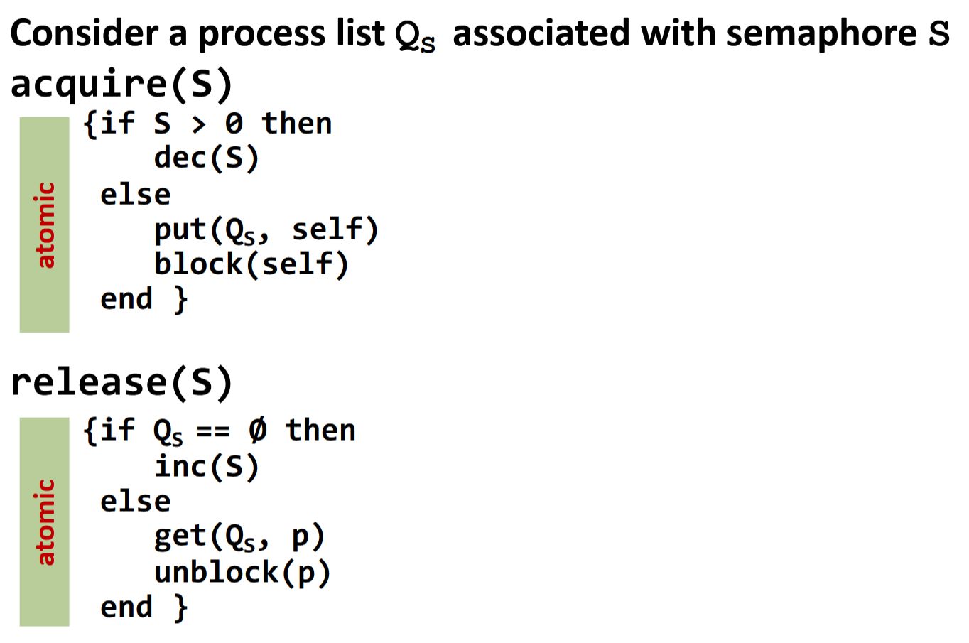
The condition test plus queue operation must be
atomic (e.g. under an internal lock).
release only increments
S if
no one is waiting: otherwise it directly unblocks a waiting process without S ever becoming positive.
Back
ETH::2._Semester::PProg::12._Shared_Memory_Concurrency::8._Semaphores
Implementation of a semaphore without
spinning (with a blocking queue \(Q_S\)):
The condition test plus queue operation must be
atomic (e.g. under an internal lock).
release only increments
S if
no one is waiting: otherwise it directly unblocks a waiting process without S ever becoming positive.
Advantage over busy-wait: waiting threads consume no CPU. The price is context-switch overhead, which only pays off once waits are long enough to dwarf it (short critical sections may still favour spinning).
Field-by-field Comparison
| Field |
Before |
After |
| Text |
Implementation of a semaphore {{c1::without spinning (with a blocking queue \(Q_S\))}}: <pre>acquire(S): release(S):
if S > 0: dec(S) if Q_S == \(\emptyset\): inc(S)
else: put(Q_S, self); else: get(Q_S, p);
block(self) unblock(p)</pre>The condition test plus queue operation must be {{c2::atomic}} (e.g. under an internal lock). {{c3::<code>release</code> only increments <code>S</code> if no one is waiting}}: otherwise it directly unblocks a waiting process without <code>S</code> ever becoming positive. |
Implementation of a semaphore without {{c1::spinning (with a blocking queue \(Q_S\))}}: <pre><img src="paste-f2c4bd33e27d75d01b7fe526db4f7ca2939ae39b.jpg"><br></pre>The condition test plus queue operation must be {{c2::atomic (e.g. under an internal lock)}}. <br><code>release</code> only increments <code>S</code> if {{c3::no one is waiting: otherwise it directly unblocks a waiting process without <code>S</code> ever becoming positive}}. |
Tags:
ETH::2._Semester::PProg::12._Shared_Memory_Concurrency::8._Semaphores
Note 36: ETH::2. Semester::PProg
Deck: ETH::2. Semester::PProg
Note Type: Horvath Cloze
GUID: +YN}l=~9iw
modified
Before
Front
ETH::2._Semester::PProg::12._Shared_Memory_Concurrency::5._Locks_with_Atomic_Registers
Mutual exclusion built only from atomic registers (Filter, Bakery, Peterson) is not used in practice for four reasons: space lower bound is linear in the maximum number of threads; correctness relies on no memory reordering, which requires expensive memory barriers in real hardware; these algorithms are not wait-free; the "primitive" assumption is unrealistic - hardware provides faster combined RMW instructions instead.
Back
ETH::2._Semester::PProg::12._Shared_Memory_Concurrency::5._Locks_with_Atomic_Registers
Mutual exclusion built only from atomic registers (Filter, Bakery, Peterson) is not used in practice for four reasons: space lower bound is linear in the maximum number of threads; correctness relies on no memory reordering, which requires expensive memory barriers in real hardware; these algorithms are not wait-free; the "primitive" assumption is unrealistic - hardware provides faster combined RMW instructions instead.
The way out: extend the model. Modern multiprocessor architectures provide special instructions for atomically reading and writing at once (TAS, CAS, LL/SC), enabling \(O(1)\) space mutexes with practical performance.
After
Front
ETH::2._Semester::PProg::12._Shared_Memory_Concurrency::5._Locks_with_Atomic_Registers
Mutual exclusion built only from atomic registers (Filter, Bakery, Peterson) is not used in practice for four reasons:
- Space lower bound is linear in the maximum number of threads.
- Correctness relies on no memory reordering, which requires expensive memory barriers in real hardware.
- These algorithms are not wait-free.
- The "primitive" assumption is unrealistic - hardware provides faster combined RMW instructions instead.
Back
ETH::2._Semester::PProg::12._Shared_Memory_Concurrency::5._Locks_with_Atomic_Registers
Mutual exclusion built only from atomic registers (Filter, Bakery, Peterson) is not used in practice for four reasons:
- Space lower bound is linear in the maximum number of threads.
- Correctness relies on no memory reordering, which requires expensive memory barriers in real hardware.
- These algorithms are not wait-free.
- The "primitive" assumption is unrealistic - hardware provides faster combined RMW instructions instead.
The way out: extend the model. Modern multiprocessor architectures provide special instructions for atomically reading and writing at once (TAS, CAS, LL/SC), enabling \(O(1)\) space mutexes with practical performance.
Field-by-field Comparison
| Field |
Before |
After |
| Text |
Mutual exclusion built only from atomic registers (Filter, Bakery, Peterson) is not used in practice for four reasons: {{c1::space lower bound is linear in the maximum number of threads}}; {{c1::correctness relies on no memory reordering, which requires expensive memory barriers in real hardware}}; {{c1::these algorithms are not wait-free}}; {{c1::the "primitive" assumption is unrealistic - hardware provides faster combined RMW instructions instead}}. |
Mutual exclusion built only from atomic registers (Filter, Bakery, Peterson) is not used in practice for four reasons: <br><ol><li>{{c1::Space lower bound is linear in the maximum number of threads}}.</li><li>{{c2::Correctness relies on no memory reordering, which requires expensive memory barriers in real hardware}}.</li><li>{{c3::These algorithms are not wait-free}}.</li><li>{{c4::The "primitive" assumption is unrealistic - hardware provides faster combined RMW instructions instead}}.</li></ol> |
Tags:
ETH::2._Semester::PProg::12._Shared_Memory_Concurrency::5._Locks_with_Atomic_Registers
Note 37: ETH::2. Semester::PProg
Deck: ETH::2. Semester::PProg
Note Type: Horvath Cloze
GUID: /J$dsYJ
modified
Before
Front
ETH::2._Semester::PProg::12._Shared_Memory_Concurrency::9._Barriers
A barrier synchronises a number \(n\) of processes such that no process passes the barrier until all \(n\) of them have reached it.
Back
ETH::2._Semester::PProg::12._Shared_Memory_Concurrency::9._Barriers
A barrier synchronises a number \(n\) of processes such that no process passes the barrier until all \(n\) of them have reached it.
Unlike a rendezvous (which is for exactly two processes), a barrier generalises to arbitrarily many. This fits BSP naturally: between any two supersteps stands a barrier.
After
Front
ETH::2._Semester::PProg::12._Shared_Memory_Concurrency::9._Barriers
A barrier synchronises a number \(n\) of processes such that no process passes the .
Back
ETH::2._Semester::PProg::12._Shared_Memory_Concurrency::9._Barriers
A barrier synchronises a number \(n\) of processes such that no process passes the .
Unlike a rendezvous (which is for exactly two processes), a barrier generalises to arbitrarily many. This fits BSP naturally: between any two supersteps stands a barrier.
Field-by-field Comparison
| Field |
Before |
After |
| Text |
A {{c1::barrier}} synchronises {{c2::a number \(n\) of processes such that no process passes the barrier until all \(n\) of them have reached it}}. |
A {{c1::barrier}} synchronises {{c2::a number \(n\) of processes such that no process passes the {{c1::barrier}} until all \(n\) of them have reached it}}. |
Tags:
ETH::2._Semester::PProg::12._Shared_Memory_Concurrency::9._Barriers
Note 38: ETH::2. Semester::PProg
Deck: ETH::2. Semester::PProg
Note Type: Horvath Cloze
GUID: 0~]{jI&/:2
modified
Before
Front
ETH::2._Semester::PProg::12._Shared_Memory_Concurrency::5._Locks_with_Atomic_Registers
The
Filter Lock extends Peterson's lock from 2 to \(n\) processes by introducing
\(n-1\) levels: each thread climbs from level 1 up to level \(n-1\), and at each level \(\ell\) it sets
level[me] = \ell and
victim[\ell] = me, then waits while
\exists k \neq me: level[k] >= \ell && victim[\ell] == me
Back
ETH::2._Semester::PProg::12._Shared_Memory_Concurrency::5._Locks_with_Atomic_Registers
The
Filter Lock extends Peterson's lock from 2 to \(n\) processes by introducing
\(n-1\) levels: each thread climbs from level 1 up to level \(n-1\), and at each level \(\ell\) it sets
level[me] = \ell and
victim[\ell] = me, then waits while
\exists k \neq me: level[k] >= \ell && victim[\ell] == me
Intuition: at each level, Peterson's mechanism filters out at most one thread (the current victim, if anyone else is still around). After traversing all \(n-1\) levels, at most one thread can be left, which then enters the CS.
unlock just resets level[me] = 0.
After
Front
ETH::2._Semester::PProg::12._Shared_Memory_Concurrency::5._Locks_with_Atomic_Registers
The Filter Lock extends Peterson's lock from 2 to \(n\) processes by introducing \(n-1\) levels:
Each thread climbs from level 1 up to level \(n-1\), and at each level \(\ell\) it sets \(\texttt{level[me]} = \ell\) and \(\texttt{victim}[\ell] = \texttt{me}\), then waits while
\(\exists k \neq \texttt{me}: \texttt{level}[k] \geq \ell \;\land\; \texttt{victim}[\ell] = \texttt{me}\)
Back
ETH::2._Semester::PProg::12._Shared_Memory_Concurrency::5._Locks_with_Atomic_Registers
The Filter Lock extends Peterson's lock from 2 to \(n\) processes by introducing \(n-1\) levels:
Each thread climbs from level 1 up to level \(n-1\), and at each level \(\ell\) it sets \(\texttt{level[me]} = \ell\) and \(\texttt{victim}[\ell] = \texttt{me}\), then waits while
\(\exists k \neq \texttt{me}: \texttt{level}[k] \geq \ell \;\land\; \texttt{victim}[\ell] = \texttt{me}\)
Intuition: at each level, Peterson's mechanism filters out at most one thread (the current victim, if anyone else is still around). After traversing all \(n-1\) levels, at most one thread can be left, which then enters the CS.
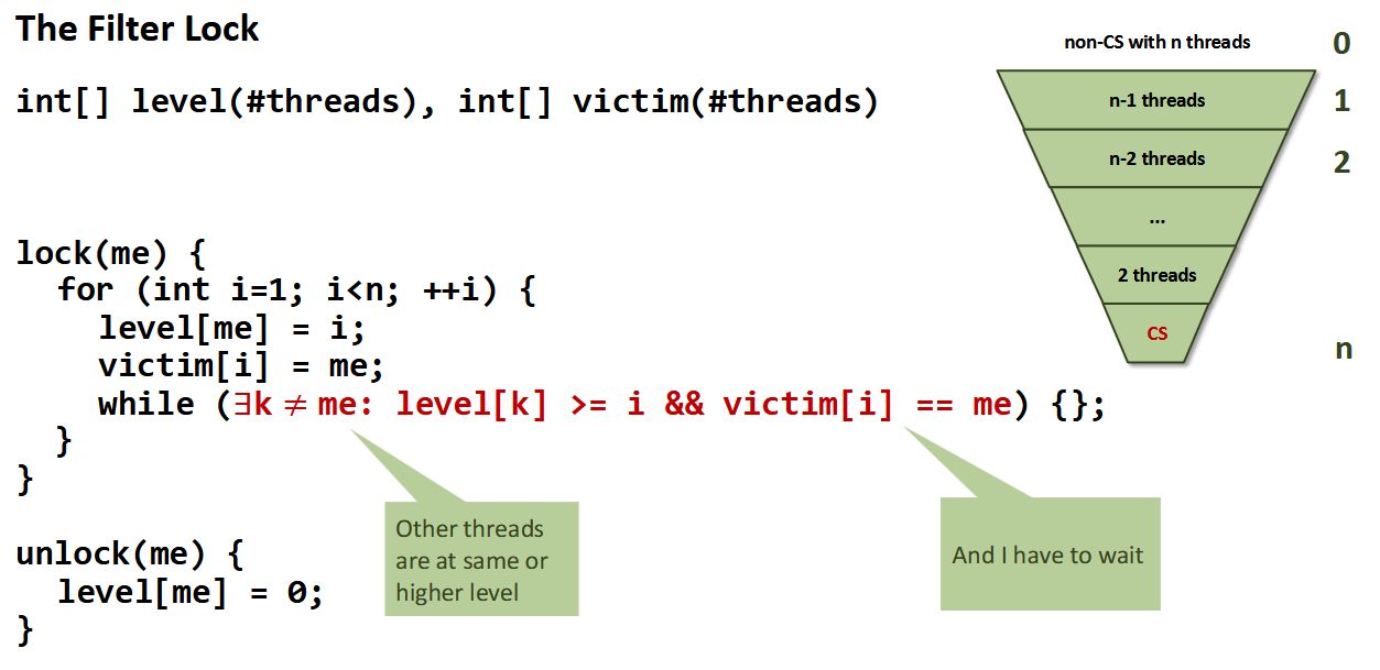
unlock just resets
level[me] = 0.
Field-by-field Comparison
| Field |
Before |
After |
| Text |
The {{c1::Filter Lock}} extends Peterson's lock from 2 to \(n\) processes by introducing {{c2::\(n-1\) levels}}: each thread climbs from level 1 up to level \(n-1\), and at each level \(\ell\) it sets <code>level[me] = \ell</code> and <code>victim[\ell] = me</code>, then waits while <pre>\exists k \neq me: level[k] >= \ell && victim[\ell] == me</pre> |
The {{c1::Filter Lock}} extends Peterson's lock from 2 to \(n\) processes by introducing {{c2::\(n-1\) levels}}: <br>Each thread climbs from level 1 up to level \(n-1\), and at each level \(\ell\) it sets \(\texttt{level[me]} = \ell\) and \(\texttt{victim}[\ell] = \texttt{me}\), then waits while <br>\(\exists k \neq \texttt{me}: \texttt{level}[k] \geq \ell \;\land\; \texttt{victim}[\ell] = \texttt{me}\) |
| Extra |
Intuition: at each level, Peterson's mechanism filters out at most one thread (the current victim, if anyone else is still around). After traversing all \(n-1\) levels, at most one thread can be left, which then enters the CS.<br><br><code>unlock</code> just resets <code>level[me] = 0</code>. |
Intuition: at each level, Peterson's mechanism filters out at most one thread (the current victim, if anyone else is still around). After traversing all \(n-1\) levels, at most one thread can be left, which then enters the CS.<br><br><img src="paste-be547b78f721e9fb57a587d379ea29ddb769e437.jpg"><br><br><code>unlock</code> just resets <code>level[me] = 0</code>. |
Tags:
ETH::2._Semester::PProg::12._Shared_Memory_Concurrency::5._Locks_with_Atomic_Registers
Note 39: ETH::2. Semester::PProg
Deck: ETH::2. Semester::PProg
Note Type: Horvath Cloze
GUID: 4%UUWqRVem
modified
Before
Front
ETH::2._Semester::PProg::12._Shared_Memory_Concurrency::7._Deadlock_Avoidance
When applying resource ordering and the objects do not have a natural total order, generate one: each instance is assigned a unique final long index from a class-level AtomicLong counter via counter.incrementAndGet() in the constructor. Locks are then always acquired in ascending order of index.
Back
ETH::2._Semester::PProg::12._Shared_Memory_Concurrency::7._Deadlock_Avoidance
When applying resource ordering and the objects do not have a natural total order, generate one: each instance is assigned a unique final long index from a class-level AtomicLong counter via counter.incrementAndGet() in the constructor. Locks are then always acquired in ascending order of index.
This is the standard pattern used inside java.util.concurrent. AtomicLong guarantees uniqueness and monotonicity even under concurrent construction, and a 64-bit counter never realistically overflows.
Using System.identityHashCode is tempting but unsafe - hashes can collide.
After
Front
ETH::2._Semester::PProg::12._Shared_Memory_Concurrency::7._Deadlock_Avoidance
When applying resource ordering and the objects do not have a natural total order, generate one:
Each instance is assigned a unique final long index from a class-level AtomicLong counter via counter.incrementAndGet() in the constructor.
Locks are then always acquired in ascending order of index.
Back
ETH::2._Semester::PProg::12._Shared_Memory_Concurrency::7._Deadlock_Avoidance
When applying resource ordering and the objects do not have a natural total order, generate one:
Each instance is assigned a unique final long index from a class-level AtomicLong counter via counter.incrementAndGet() in the constructor.
Locks are then always acquired in ascending order of index.
This is the standard pattern used inside
java.util.concurrent.
AtomicLong guarantees uniqueness and monotonicity even under concurrent construction, and a 64-bit counter never realistically overflows.
Using
System.identityHashCode is tempting but unsafe - hashes can collide.
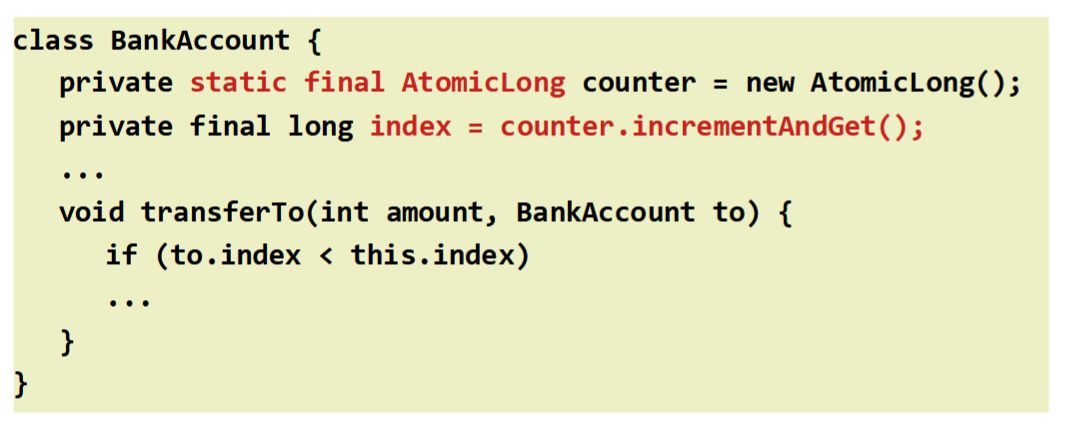
Field-by-field Comparison
| Field |
Before |
After |
| Text |
When applying resource ordering and the objects do not have a natural total order, generate one: each instance is assigned {{c1::a unique <code>final long</code> index from a class-level <code>AtomicLong counter</code>}} via <code>counter.incrementAndGet()</code> in the constructor. Locks are then always acquired in {{c2::ascending order of <code>index</code>}}. |
When applying resource ordering and the objects do not have a natural total order, generate one: <br>{{c1::Each instance is assigned a unique <code>final long</code> index from a class-level <code>AtomicLong counter</code> via <code>counter.incrementAndGet()</code> in the constructor. <br>Locks are then always acquired in ascending order of <code>index</code>}}. |
| Extra |
This is the standard pattern used inside <code>java.util.concurrent</code>. <code>AtomicLong</code> guarantees uniqueness and monotonicity even under concurrent construction, and a 64-bit counter never realistically overflows.<br><br>Using <code>System.identityHashCode</code> is tempting but unsafe - hashes can collide. |
This is the standard pattern used inside <code>java.util.concurrent</code>. <code>AtomicLong</code> guarantees uniqueness and monotonicity even under concurrent construction, and a 64-bit counter never realistically overflows.<br><br>Using <code>System.identityHashCode</code> is tempting but unsafe - hashes can collide.<br><br><img src="paste-a4af20ca247ce047f7595067e7cadac74b99884e.jpg"> |
Tags:
ETH::2._Semester::PProg::12._Shared_Memory_Concurrency::7._Deadlock_Avoidance
Note 40: ETH::2. Semester::PProg
Deck: ETH::2. Semester::PProg
Note Type: Horvath Cloze
GUID: 6>tVnB+D6%
modified
Before
Front
ETH::2._Semester::PProg::12._Shared_Memory_Concurrency::9._Barriers
Correct (one-shot) barrier with semaphores
mutex = 1,
barrier = 0 and integer
count = 0:
acquire(mutex)
count++
release(mutex)
if (count == n) release(barrier)
acquire(barrier)
release(barrier)
The mutex protects
the race on count++; the trailing
acquire(barrier); release(barrier); is called a
turnstile and ensures that
each thread that gets through immediately admits the next, so all \(n\) threads pass in sequence.
Back
ETH::2._Semester::PProg::12._Shared_Memory_Concurrency::9._Barriers
Correct (one-shot) barrier with semaphores
mutex = 1,
barrier = 0 and integer
count = 0:
acquire(mutex)
count++
release(mutex)
if (count == n) release(barrier)
acquire(barrier)
release(barrier)
The mutex protects
the race on count++; the trailing
acquire(barrier); release(barrier); is called a
turnstile and ensures that
each thread that gets through immediately admits the next, so all \(n\) threads pass in sequence.
After one run, count = n and barrier = 1: the barrier is not reusable (a reusable version needs a second phase, often called a "two-phase barrier"). Exactly one thread (the \(n\)-th) calls release(barrier), and the turnstile passes the token along.
After
Front
ETH::2._Semester::PProg::12._Shared_Memory_Concurrency::9._Barriers
Correct (one-shot) barrier with semaphores
mutex = 1,
barrier = 0 and integer
count = 0:
acquire(mutex)
count++
release(mutex)
if (count == n) release(barrier)
acquire(barrier)
release(barrier)
The mutex protects
the race on count++.
The trailing
acquire(barrier); release(barrier); is called a
turnstile and ensures that
each thread that gets through immediately admits the next, so all \(n\) threads pass in sequence.
Back
ETH::2._Semester::PProg::12._Shared_Memory_Concurrency::9._Barriers
Correct (one-shot) barrier with semaphores
mutex = 1,
barrier = 0 and integer
count = 0:
acquire(mutex)
count++
release(mutex)
if (count == n) release(barrier)
acquire(barrier)
release(barrier)
The mutex protects
the race on count++.
The trailing
acquire(barrier); release(barrier); is called a
turnstile and ensures that
each thread that gets through immediately admits the next, so all \(n\) threads pass in sequence.
After one run, count = n and barrier = 1: the barrier is not reusable (a reusable version needs a second phase, often called a "two-phase barrier"). Exactly one thread (the \(n\)-th) calls release(barrier), and the turnstile passes the token along.
Field-by-field Comparison
| Field |
Before |
After |
| Text |
Correct (one-shot) barrier with semaphores <code>mutex = 1</code>, <code>barrier = 0</code> and integer <code>count = 0</code>: <pre>acquire(mutex)
count++
release(mutex)
if (count == n) release(barrier)
acquire(barrier)
release(barrier)</pre>The mutex protects {{c1::the race on <code>count++</code>}}; the trailing <code>acquire(barrier); release(barrier);</code> is called a {{c2::turnstile}} and ensures that {{c3::each thread that gets through immediately admits the next, so all \(n\) threads pass in sequence}}. |
Correct (one-shot) barrier with semaphores <code>mutex = 1</code>, <code>barrier = 0</code> and integer <code>count = 0</code>: <pre>acquire(mutex)
count++
release(mutex)
if (count == n) release(barrier)
acquire(barrier)
release(barrier)</pre>The mutex protects {{c1::the race on <code>count++</code>}}. <br>The trailing <code>acquire(barrier); release(barrier);</code> is called a {{c2::turnstile}} and ensures that {{c2::each thread that gets through immediately admits the next, so all \(n\) threads pass in sequence}}. |
Tags:
ETH::2._Semester::PProg::12._Shared_Memory_Concurrency::9._Barriers
Note 41: ETH::2. Semester::PProg
Deck: ETH::2. Semester::PProg
Note Type: Horvath Cloze
GUID: 7/+$V!A5-^
modified
Before
Front
ETH::2._Semester::PProg::12._Shared_Memory_Concurrency::6._Locks_with_Atomic_Operations
java.util.concurrent.atomic.AtomicBoolean exposes two key RMW operations on top of plain get / set: compareAndSet(expect, update), which atomically writes update iff the current value equals expect and returns true on success; and getAndSet(newValue), which atomically writes newValue and returns the previous value.
Back
ETH::2._Semester::PProg::12._Shared_Memory_Concurrency::6._Locks_with_Atomic_Operations
java.util.concurrent.atomic.AtomicBoolean exposes two key RMW operations on top of plain get / set: compareAndSet(expect, update), which atomically writes update iff the current value equals expect and returns true on success; and getAndSet(newValue), which atomically writes newValue and returns the previous value.
compareAndSet ≅ CAS, getAndSet ≅ TAS. Note: even though they are called "atomic", the JLS does not guarantee these map to a single hardware instruction; they may be implemented via internal locks. They are guaranteed atomic, not guaranteed lock-free.
After
Front
ETH::2._Semester::PProg::12._Shared_Memory_Concurrency::6._Locks_with_Atomic_Operations
java.util.concurrent.atomic.AtomicBoolean exposes two key RMW operations on top of plain
get /
set:
compareAndSet(expect, update), which atomically writes update iff the current value equals expect and returns true on success.getAndSet(newValue), which atomically writes newValue and returns the previous value.
Back
ETH::2._Semester::PProg::12._Shared_Memory_Concurrency::6._Locks_with_Atomic_Operations
java.util.concurrent.atomic.AtomicBoolean exposes two key RMW operations on top of plain
get /
set:
compareAndSet(expect, update), which atomically writes update iff the current value equals expect and returns true on success.getAndSet(newValue), which atomically writes newValue and returns the previous value.
compareAndSet ≅ CAS, getAndSet ≅ TAS.
Note: even though they are called "atomic", the JLS does not guarantee these map to a single hardware instruction; they may be implemented via internal locks. They are guaranteed atomic, not guaranteed lock-free.
Field-by-field Comparison
| Field |
Before |
After |
| Text |
<code>java.util.concurrent.atomic.AtomicBoolean</code> exposes two key RMW operations on top of plain <code>get</code> / <code>set</code>: {{c1::<code>compareAndSet(expect, update)</code>}}, which atomically writes <code>update</code> iff the current value equals <code>expect</code> and {{c2::returns <code>true</code> on success}}; and {{c3::<code>getAndSet(newValue)</code>}}, which {{c4::atomically writes <code>newValue</code> and returns the previous value}}. |
<code>java.util.concurrent.atomic.AtomicBoolean</code> exposes two key RMW operations on top of plain <code>get</code> / <code>set</code>: <br><ol><li>{{c1::<code>compareAndSet(expect, update)</code>}}, which atomically writes <code>update</code> iff the current value equals <code>expect</code> and returns <code>true</code> on success.</li><li>{{c2::<code>getAndSet(newValue)</code>}}, which atomically writes <code>newValue</code> and returns the previous value.</li></ol> |
| Extra |
<code>compareAndSet</code> ≅ CAS, <code>getAndSet</code> ≅ TAS. Note: even though they are called "atomic", the JLS does not guarantee these map to a single hardware instruction; they may be implemented via internal locks. They are guaranteed atomic, not guaranteed lock-free. |
<code>compareAndSet</code> ≅ CAS, <code>getAndSet</code> ≅ TAS. <br><br>Note: even though they are called "atomic", the JLS does not guarantee these map to a single hardware instruction; they may be implemented via internal locks. They are guaranteed atomic, not guaranteed lock-free. |
Tags:
ETH::2._Semester::PProg::12._Shared_Memory_Concurrency::6._Locks_with_Atomic_Operations
Note 42: ETH::2. Semester::PProg
Deck: ETH::2. Semester::PProg
Note Type: Horvath Cloze
GUID:
modified
Before
Front
ETH::2._Semester::PProg::12._Shared_Memory_Concurrency::8._Semaphores
Scaled dot product \(x = (a^T \cdot d) \cdot z\) with partial sums \(x_A, x_B\) on two threads: with locks (lock(); x = x + x_A; unlock(); in both threads) it is unclear when \(x\) is finished. With a semaphore \(S\) initialised to \(0\), the order can be enforced: thread A computes x = x + x_A and then calls release(S); thread B does acquire(S) first, then x = x + x_B, then x = x*z. This guarantees that A adds before B.
Back
ETH::2._Semester::PProg::12._Shared_Memory_Concurrency::8._Semaphores
Scaled dot product \(x = (a^T \cdot d) \cdot z\) with partial sums \(x_A, x_B\) on two threads: with locks (lock(); x = x + x_A; unlock(); in both threads) it is unclear when \(x\) is finished. With a semaphore \(S\) initialised to \(0\), the order can be enforced: thread A computes x = x + x_A and then calls release(S); thread B does acquire(S) first, then x = x + x_B, then x = x*z. This guarantees that A adds before B.
This is exactly what locks cannot deliver: not only mutual exclusion, but a concrete ordering between threads. The trick with initial value \(0\): the first acquire blocks until a release unblocks it: the semaphore is used as a signal, not as a mutex.
After
Front
ETH::2._Semester::PProg::12._Shared_Memory_Concurrency::8._Semaphores
Scaled dot product \(x = (a^T \cdot d) \cdot z\) with partial sums \(x_A, x_B\) on two threads:
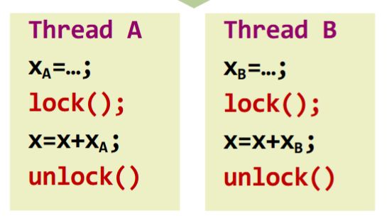
With locks it is unclear
when \(x\) is finished.
With a semaphore \(S\) initialised to \(0\), the order can be enforced:
thread A computes x = x + x_A and then calls release(S);
thread B does acquire(S) first, then x = x + x_B, then x = x*z. This guarantees that A adds before B.
Back
ETH::2._Semester::PProg::12._Shared_Memory_Concurrency::8._Semaphores
Scaled dot product \(x = (a^T \cdot d) \cdot z\) with partial sums \(x_A, x_B\) on two threads:
With locks it is unclear
when \(x\) is finished.
With a semaphore \(S\) initialised to \(0\), the order can be enforced:
thread A computes x = x + x_A and then calls release(S);
thread B does acquire(S) first, then x = x + x_B, then x = x*z. This guarantees that A adds before B.
This is exactly what locks cannot deliver: not only mutual exclusion, but a concrete ordering between threads. The trick with initial value \(0\): the first
acquire blocks until a
release unblocks it: the semaphore is used as a
signal, not as a mutex.
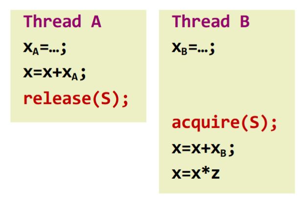
Field-by-field Comparison
| Field |
Before |
After |
| Text |
Scaled dot product \(x = (a^T \cdot d) \cdot z\) with partial sums \(x_A, x_B\) on two threads: with locks ({{c1::<code>lock(); x = x + x_A; unlock();</code> in both threads}}) it is unclear <i>when</i> \(x\) is finished. With a semaphore \(S\) initialised to \(0\), the order can be enforced: {{c2::thread A computes <code>x = x + x_A</code> and then calls <code>release(S)</code>}}; {{c2::thread B does <code>acquire(S)</code> first, then <code>x = x + x_B</code>, then <code>x = x*z</code>}}. This guarantees that A adds before B. |
Scaled dot product \(x = (a^T \cdot d) \cdot z\) with partial sums \(x_A, x_B\) on two threads: <br><br><img src="paste-aa2db79945226e156083dee46d13de4b6bc7698e.jpg"><br><br>With locks it is unclear {{c1::<i>when</i> \(x\) is finished}}. <br><br>With a semaphore \(S\) initialised to \(0\), the order can be enforced: {{c2::thread A computes <code>x = x + x_A</code> and then calls <code>release(S)</code>}}; {{c2::thread B does <code>acquire(S)</code> first, then <code>x = x + x_B</code>, then <code>x = x*z</code>}}. This guarantees that A adds before B. |
| Extra |
This is exactly what locks cannot deliver: not only mutual exclusion, but a concrete ordering between threads. The trick with initial value \(0\): the first <code>acquire</code> blocks until a <code>release</code> unblocks it: the semaphore is used as a <em>signal</em>, not as a mutex. |
This is exactly what locks cannot deliver: not only mutual exclusion, but a concrete ordering between threads. The trick with initial value \(0\): the first <code>acquire</code> blocks until a <code>release</code> unblocks it: the semaphore is used as a <em>signal</em>, not as a mutex.<br><br><img src="paste-ac1e6ceaf2129092ac601dfea415d4620ac16889.jpg"> |
Tags:
ETH::2._Semester::PProg::12._Shared_Memory_Concurrency::8._Semaphores
Note 43: ETH::2. Semester::PProg
Deck: ETH::2. Semester::PProg
Note Type: Horvath Cloze
GUID: >^UKYB#lC@
modified
Before
Front
ETH::2._Semester::PProg::12._Shared_Memory_Concurrency::9._Barriers
A naive reusable barrier extends the one-shot barrier with a symmetric "second half"
acquire(mutex); count--; release(mutex);
if (count==0) acquire(barrier);
after the turnstile, intended to reset
count and
barrier. It is broken because
the invariant "after all processes have passed, barrier = 0" is violated: release(barrier) can be executed multiple times across iterations before any thread reaches the resetting acquire(barrier), so barrier drifts to \(2, 3, \dots\), and
the if (count == 0) acquire(barrier) check happens outside the mutex, so it cannot reliably restore the semaphore to 0 in the presence of fast re-entrants.
Back
ETH::2._Semester::PProg::12._Shared_Memory_Concurrency::9._Barriers
A naive reusable barrier extends the one-shot barrier with a symmetric "second half"
acquire(mutex); count--; release(mutex);
if (count==0) acquire(barrier);
after the turnstile, intended to reset
count and
barrier. It is broken because
the invariant "after all processes have passed, barrier = 0" is violated: release(barrier) can be executed multiple times across iterations before any thread reaches the resetting acquire(barrier), so barrier drifts to \(2, 3, \dots\), and
the if (count == 0) acquire(barrier) check happens outside the mutex, so it cannot reliably restore the semaphore to 0 in the presence of fast re-entrants.
Concrete scheduling: thread A finishes phase 1 with count = 1; meanwhile B and C race into the next iteration, both increment count back up, hit count == n, and each calls release(barrier). The semaphore is no longer a clean 0/1 toggle. The fix is a proper two-phase split with separate semaphores for the two halves.
After
Front
ETH::2._Semester::PProg::12._Shared_Memory_Concurrency::9._Barriers
A naive reusable barrier extends the one-shot barrier with a symmetric "second half"
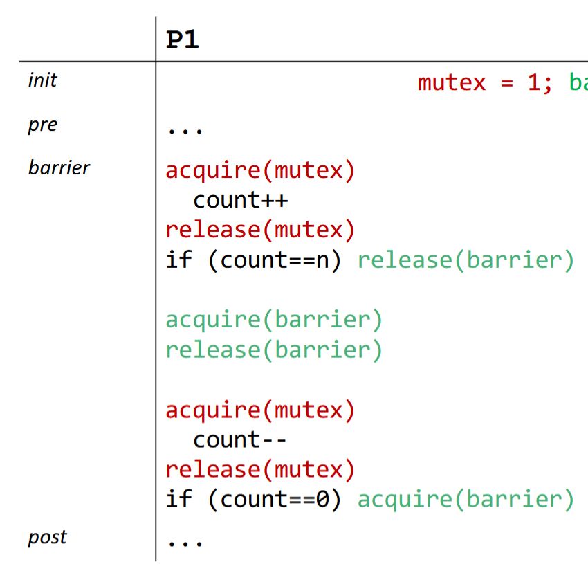
after the turnstile, intended to reset
count and
barrier.
It is broken because the invariant
"after all processes have passed, barrier = 0" is violated: release(barrier) can be executed multiple times across iterations before any thread reaches the resetting acquire(barrier), so barrier drifts to \(2, 3, \dots\), and the
if (count == 0) acquire(barrier) check
happens outside the mutex, so it cannot reliably restore the semaphore to 0 in the presence of fast re-entrants.
Back
ETH::2._Semester::PProg::12._Shared_Memory_Concurrency::9._Barriers
A naive reusable barrier extends the one-shot barrier with a symmetric "second half"
after the turnstile, intended to reset
count and
barrier.
It is broken because the invariant
"after all processes have passed, barrier = 0" is violated: release(barrier) can be executed multiple times across iterations before any thread reaches the resetting acquire(barrier), so barrier drifts to \(2, 3, \dots\), and the
if (count == 0) acquire(barrier) check
happens outside the mutex, so it cannot reliably restore the semaphore to 0 in the presence of fast re-entrants.
Concrete scheduling: thread A finishes phase 1 with count = 1; meanwhile B and C race into the next iteration, both increment count back up, hit count == n, and each calls release(barrier). The semaphore is no longer a clean 0/1 toggle. The fix is a proper two-phase split with separate semaphores for the two halves.
Field-by-field Comparison
| Field |
Before |
After |
| Text |
A naive reusable barrier extends the one-shot barrier with a symmetric "second half" <pre>acquire(mutex); count--; release(mutex);
if (count==0) acquire(barrier);</pre>after the turnstile, intended to reset <code>count</code> and <code>barrier</code>. It is broken because {{c1::the invariant "after all processes have passed, <code>barrier = 0</code>" is violated: <code>release(barrier)</code> can be executed multiple times across iterations before any thread reaches the resetting <code>acquire(barrier)</code>, so <code>barrier</code> drifts to \(2, 3, \dots\)}}, and {{c2::the <code>if (count == 0) acquire(barrier)</code> check happens outside the mutex, so it cannot reliably restore the semaphore to 0 in the presence of fast re-entrants}}. |
A naive reusable barrier extends the one-shot barrier with a symmetric "second half" <pre><img src="paste-ffd6359913f85c1da896aba5205bc4cf259dbbc3.jpg"><br></pre>after the turnstile, intended to reset <code>count</code> and <code>barrier</code>. <br><br>It is broken because the invariant {{c1::"after all processes have passed, <code>barrier = 0</code>" is violated: <code>release(barrier)</code> can be executed multiple times across iterations before any thread reaches the resetting <code>acquire(barrier)</code>, so <code>barrier</code> drifts to \(2, 3, \dots\)}}, and the <code>if (count == 0) acquire(barrier)</code> check {{c2::happens outside the mutex, so it cannot reliably restore the semaphore to 0 in the presence of fast re-entrants}}. |
Tags:
ETH::2._Semester::PProg::12._Shared_Memory_Concurrency::9._Barriers
Note 44: ETH::2. Semester::PProg
Deck: ETH::2. Semester::PProg
Note Type: Horvath Cloze
GUID: ApSiaX&)Ab
modified
Before
Front
ETH::2._Semester::PProg::12._Shared_Memory_Concurrency::5._Locks_with_Atomic_Registers
Lamport's Bakery algorithm solves \(n\)-process mutex by assigning each thread a
ticket (label) larger than all outstanding tickets:
flag[me] = true;
label[me] = max(label[0..n-1]) + 1;
while(\exists k != me: flag[k] && (k, label[k]) <_l (me, label[me])) {};
where ties are broken by
lexicographic order on (thread id, label), so two equal labels are still totally ordered.
Back
ETH::2._Semester::PProg::12._Shared_Memory_Concurrency::5._Locks_with_Atomic_Registers
Lamport's Bakery algorithm solves \(n\)-process mutex by assigning each thread a
ticket (label) larger than all outstanding tickets:
flag[me] = true;
label[me] = max(label[0..n-1]) + 1;
while(\exists k != me: flag[k] && (k, label[k]) <_l (me, label[me])) {};
where ties are broken by
lexicographic order on (thread id, label), so two equal labels are still totally ordered.
Properties: mutual exclusion, deadlock freedom, starvation freedom, and FCFS (the doorway is the label assignment).
The bug-resistant trick is the lexicographic tie-break: two threads can read the same max simultaneously and end up with equal labels, but the smaller-id thread still goes first - no live or dead lock.
After
Front
ETH::2._Semester::PProg::12._Shared_Memory_Concurrency::5._Locks_with_Atomic_Registers
Lamport's Bakery algorithm solves \(n\)-process mutex by assigning each thread a
ticket (label) larger than all outstanding tickets:
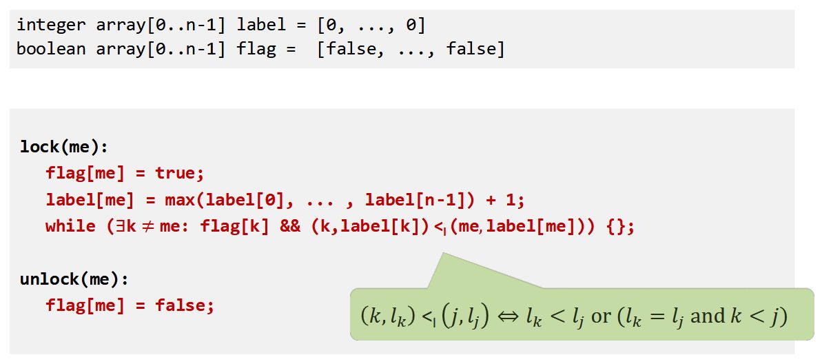
where ties are broken by
lexicographic order on (thread id, label), so two equal labels are still totally ordered.
Back
ETH::2._Semester::PProg::12._Shared_Memory_Concurrency::5._Locks_with_Atomic_Registers
Lamport's Bakery algorithm solves \(n\)-process mutex by assigning each thread a
ticket (label) larger than all outstanding tickets:
where ties are broken by
lexicographic order on (thread id, label), so two equal labels are still totally ordered.
Properties: mutual exclusion, deadlock freedom, starvation freedom, and FCFS (the doorway is the label assignment).
The bug-resistant trick is the lexicographic tie-break: two threads can read the same max simultaneously and end up with equal labels, but the smaller-id thread still goes first - no live or dead lock.
Field-by-field Comparison
| Field |
Before |
After |
| Text |
{{c1::Lamport's Bakery algorithm}} solves \(n\)-process mutex by assigning each thread a {{c2::ticket (label) larger than all outstanding tickets}}: <pre>flag[me] = true;
label[me] = max(label[0..n-1]) + 1;
while(\exists k != me: flag[k] && (k, label[k]) <_l (me, label[me])) {};</pre> where ties are broken by {{c3::lexicographic order on (thread id, label), so two equal labels are still totally ordered}}. |
{{c1::Lamport's Bakery algorithm}} solves \(n\)-process mutex by assigning each thread a {{c2::ticket (label) larger than all outstanding tickets}}:<br><br><img src="paste-7781996e26f881803d8d4ab221a20d87438ffae3.jpg"><br><br>where ties are broken by {{c3::lexicographic order on (thread id, label), so two equal labels are still totally ordered}}. |
Tags:
ETH::2._Semester::PProg::12._Shared_Memory_Concurrency::5._Locks_with_Atomic_Registers
Note 45: ETH::2. Semester::PProg
Deck: ETH::2. Semester::PProg
Note Type: Horvath Cloze
GUID: C9O/B$skj#
modified
Before
Front
ETH::2._Semester::PProg::12._Shared_Memory_Concurrency::5._Locks_with_Atomic_Registers
Peterson's starvation-freedom proof is by exhaustive contradiction: assume \(P\) is stuck in its while loop forever. Then \(Q\) is in one of three cases - stuck in non-CS (then flag[Q]=false, \(P\) proceeds, contradiction); repeatedly entering and leaving its CS (each entry sets victim=Q, freezing victim away from \(P\), so \(P\) proceeds, contradiction); also stuck in its lock loop (then \(Q\) needs victim != Q, but victim can equal at most one of \(P,Q\), contradiction).
Back
ETH::2._Semester::PProg::12._Shared_Memory_Concurrency::5._Locks_with_Atomic_Registers
Peterson's starvation-freedom proof is by exhaustive contradiction: assume \(P\) is stuck in its while loop forever. Then \(Q\) is in one of three cases - stuck in non-CS (then flag[Q]=false, \(P\) proceeds, contradiction); repeatedly entering and leaving its CS (each entry sets victim=Q, freezing victim away from \(P\), so \(P\) proceeds, contradiction); also stuck in its lock loop (then \(Q\) needs victim != Q, but victim can equal at most one of \(P,Q\), contradiction).
The case split is exhaustive because these are the only three possible long-term behaviours of \(Q\) under our assumptions. Each leads to a contradiction, so \(P\) cannot be stuck.
After
Front
ETH::2._Semester::PProg::12._Shared_Memory_Concurrency::5._Locks_with_Atomic_Registers
Peterson's starvation-freedom proof is by exhaustive contradiction:
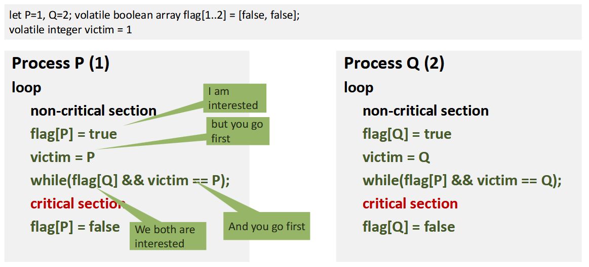
Assume \(P\) is stuck in its
while loop forever. Then \(Q\) is in one of three cases:
- Stuck in non-CS (then
flag[Q]=false, \(P\) proceeds, contradiction). - Repeatedly entering and leaving its CS (each entry sets
victim=Q, freezing victim away from \(P\), so \(P\) proceeds, contradiction). - Also stuck in its lock loop (then \(Q\) needs
victim != Q, but victim can equal at most one of \(P,Q\), contradiction).
Back
ETH::2._Semester::PProg::12._Shared_Memory_Concurrency::5._Locks_with_Atomic_Registers
Peterson's starvation-freedom proof is by exhaustive contradiction:
Assume \(P\) is stuck in its
while loop forever. Then \(Q\) is in one of three cases:
- Stuck in non-CS (then
flag[Q]=false, \(P\) proceeds, contradiction). - Repeatedly entering and leaving its CS (each entry sets
victim=Q, freezing victim away from \(P\), so \(P\) proceeds, contradiction). - Also stuck in its lock loop (then \(Q\) needs
victim != Q, but victim can equal at most one of \(P,Q\), contradiction).
The case split is exhaustive because these are the only three possible long-term behaviours of \(Q\) under our assumptions. Each leads to a contradiction, so \(P\) cannot be stuck.
Field-by-field Comparison
| Field |
Before |
After |
| Text |
Peterson's starvation-freedom proof is by exhaustive contradiction: assume \(P\) is stuck in its <code>while</code> loop forever. Then \(Q\) is in one of three cases - {{c1::stuck in non-CS (then <code>flag[Q]=false</code>, \(P\) proceeds, contradiction)}}; {{c2::repeatedly entering and leaving its CS (each entry sets <code>victim=Q</code>, freezing <code>victim</code> away from \(P\), so \(P\) proceeds, contradiction)}}; {{c3::also stuck in its lock loop (then \(Q\) needs <code>victim != Q</code>, but <code>victim</code> can equal at most one of \(P,Q\), contradiction)}}. |
Peterson's starvation-freedom proof is by exhaustive contradiction: <br><br><img src="paste-63fb713427fe3e491127bceaa3894b34b8dfc602.jpg"><br><br>Assume \(P\) is stuck in its <code>while</code> loop forever. Then \(Q\) is in one of three cases:<ol><li>{{c1::Stuck in non-CS (then <code>flag[Q]=false</code>, \(P\) proceeds, contradiction)}}.</li><li>{{c2::Repeatedly entering and leaving its CS (each entry sets <code>victim=Q</code>, freezing <code>victim</code> away from \(P\), so \(P\) proceeds, contradiction)}}.</li><li>{{c3::Also stuck in its lock loop (then \(Q\) needs <code>victim != Q</code>, but <code>victim</code> can equal at most one of \(P,Q\), contradiction)}}.</li></ol> |
Tags:
ETH::2._Semester::PProg::12._Shared_Memory_Concurrency::5._Locks_with_Atomic_Registers
Note 46: ETH::2. Semester::PProg
Deck: ETH::2. Semester::PProg
Note Type: Horvath Cloze
GUID: D|&w=l8gFV
modified
Before
Front
ETH::2._Semester::PProg::12._Shared_Memory_Concurrency::6._Locks_with_Atomic_Operations
The
Test-And-Test-And-Set (TATAS) lock improves on TAS by spinning on a plain read first:
do {
  while(state.get()) {}
} while(!state.compareAndSet(false, true));
The inner loop only
reads the cached value, generating no coherence traffic while the lock stays held; the costly RMW is attempted only
after the lock looks free.
Back
ETH::2._Semester::PProg::12._Shared_Memory_Concurrency::6._Locks_with_Atomic_Operations
The
Test-And-Test-And-Set (TATAS) lock improves on TAS by spinning on a plain read first:
do {
  while(state.get()) {}
} while(!state.compareAndSet(false, true));
The inner loop only
reads the cached value, generating no coherence traffic while the lock stays held; the costly RMW is attempted only
after the lock looks free.
Caveat: TATAS does not generalise. The classical "double-checked locking" pattern - a TATAS-style optimisation around lazy initialisation - is famously broken without explicit memory barriers, because compilers and hardware may reorder the publish of the new object with respect to the flag write.
After
Front
ETH::2._Semester::PProg::12._Shared_Memory_Concurrency::6._Locks_with_Atomic_Operations
The
Test-And-Test-And-Set (TATAS) lock improves on TAS by spinning on a plain read first:
do {
  while(state.get()) {}
} while(!state.compareAndSet(false, true));
The inner loop only
reads the cached value, generating no coherence traffic while the lock stays held; the costly RMW is attempted only
after the lock looks free.
Back
ETH::2._Semester::PProg::12._Shared_Memory_Concurrency::6._Locks_with_Atomic_Operations
The
Test-And-Test-And-Set (TATAS) lock improves on TAS by spinning on a plain read first:
do {
  while(state.get()) {}
} while(!state.compareAndSet(false, true));
The inner loop only
reads the cached value, generating no coherence traffic while the lock stays held; the costly RMW is attempted only
after the lock looks free.
Caveat: TATAS does not generalise. The classical "double-checked locking" pattern - a TATAS-style optimisation around lazy initialisation - is famously broken without explicit memory barriers, because compilers and hardware may reorder the publish of the new object with respect to the flag write.
Field-by-field Comparison
| Field |
Before |
After |
| Text |
The <i>Test-And-Test-And-Set (TATAS)</i> lock improves on TAS by spinning on a plain read first: <pre>do {
while(state.get()) {}
} while(!state.compareAndSet(false, true));</pre> The inner loop only {{c1::reads the cached value, generating no coherence traffic while the lock stays held}}; the costly RMW is attempted only {{c2::after the lock <i>looks</i> free}}. |
The <i>Test-And-Test-And-Set (TATAS)</i> lock improves on TAS by spinning on a plain read first: <pre>do {
while(state.get()) {}
} while(!state.compareAndSet(false, true));</pre> The inner loop only {{c1::reads the cached value, generating no coherence traffic while the lock stays held}}; the costly RMW is attempted only {{c1::after the lock <i>looks</i> free}}. |
Tags:
ETH::2._Semester::PProg::12._Shared_Memory_Concurrency::6._Locks_with_Atomic_Operations
Note 47: ETH::2. Semester::PProg
Deck: ETH::2. Semester::PProg
Note Type: Horvath Cloze
GUID: FGboL4isC9
modified
Before
Front
ETH::2._Semester::PProg::12._Shared_Memory_Concurrency::7._Deadlock_Avoidance
Another deadlock fix is to protect every transferTo with a single static global lock, which trivially avoids cycles because there is only one lock to acquire. Cost: no two transfers can run in parallel, even on completely disjoint pairs of accounts.
Back
ETH::2._Semester::PProg::12._Shared_Memory_Concurrency::7._Deadlock_Avoidance
Another deadlock fix is to protect every transferTo with a single static global lock, which trivially avoids cycles because there is only one lock to acquire. Cost: no two transfers can run in parallel, even on completely disjoint pairs of accounts.
This sacrifices nearly all the available concurrency for safety. It is a sensible default when contention is rare or when correctness clearly trumps throughput, but rarely the right answer at scale.
After
Front
ETH::2._Semester::PProg::12._Shared_Memory_Concurrency::7._Deadlock_Avoidance
Another deadlock fix is to protect every transferTo with a single static global lock, which trivially avoids cycles because there is only one lock to acquire.
Cost: no two transfers can run in parallel, even on completely disjoint pairs of accounts.
Back
ETH::2._Semester::PProg::12._Shared_Memory_Concurrency::7._Deadlock_Avoidance
Another deadlock fix is to protect every transferTo with a single static global lock, which trivially avoids cycles because there is only one lock to acquire.
Cost: no two transfers can run in parallel, even on completely disjoint pairs of accounts.
This sacrifices nearly all the available concurrency for safety. It is a sensible default when contention is rare or when correctness clearly trumps throughput, but rarely the right answer at scale.
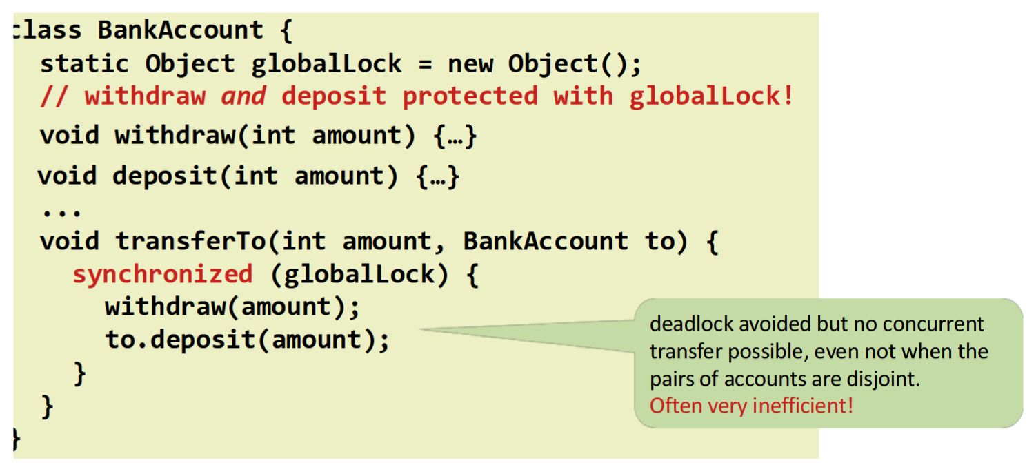
Field-by-field Comparison
| Field |
Before |
After |
| Text |
Another deadlock fix is to protect every <code>transferTo</code> with {{c1::a single static global lock}}, which trivially avoids cycles because there is only one lock to acquire. Cost: {{c2::no two transfers can run in parallel, even on completely disjoint pairs of accounts}}. |
Another deadlock fix is to protect every <code>transferTo</code> with {{c1::a single static global lock, which trivially avoids cycles because there is only one lock to acquire}}. <br><br>Cost: {{c2::no two transfers can run in parallel, even on completely disjoint pairs of accounts}}. |
| Extra |
This sacrifices nearly all the available concurrency for safety. It is a sensible default when contention is rare or when correctness clearly trumps throughput, but rarely the right answer at scale. |
This sacrifices nearly all the available concurrency for safety. It is a sensible default when contention is rare or when correctness clearly trumps throughput, but rarely the right answer at scale.<br><br><img src="paste-76071e07b5ffd7a0eb5781ab5441704540621931.jpg"> |
Tags:
ETH::2._Semester::PProg::12._Shared_Memory_Concurrency::7._Deadlock_Avoidance
Note 48: ETH::2. Semester::PProg
Deck: ETH::2. Semester::PProg
Note Type: Horvath Cloze
GUID: Fc~lyNYx7K
modified
Before
Front
ETH::2._Semester::PProg::12._Shared_Memory_Concurrency::6._Locks_with_Atomic_Operations
A naive TAS-based spinlock
while(state.getAndSet(true)) {} scales poorly because
every spinning thread issues writes to the lock variable, which
generates bus contention and forces the cache-coherence protocol to invalidate all other cached copies on every retry.
Back
ETH::2._Semester::PProg::12._Shared_Memory_Concurrency::6._Locks_with_Atomic_Operations
A naive TAS-based spinlock
while(state.getAndSet(true)) {} scales poorly because
every spinning thread issues writes to the lock variable, which
generates bus contention and forces the cache-coherence protocol to invalidate all other cached copies on every retry.
Result: the runtime per thread grows roughly linearly (or worse) with the number of contending threads. Each spinning core hammers the bus, so even threads not currently trying to acquire the lock pay a cost. The fix is to spin on a read until the lock looks free (TTAS), then attempt the RMW only optimistically.
After
Front
ETH::2._Semester::PProg::12._Shared_Memory_Concurrency::6._Locks_with_Atomic_Operations
A naive TAS-based spinlock
while(state.getAndSet(true)) {} scales poorly because
every spinning thread issues writes to the lock variable, which
generates bus contention and forces the cache-coherence protocol to invalidate all other cached copies on every retry.
Back
ETH::2._Semester::PProg::12._Shared_Memory_Concurrency::6._Locks_with_Atomic_Operations
A naive TAS-based spinlock
while(state.getAndSet(true)) {} scales poorly because
every spinning thread issues writes to the lock variable, which
generates bus contention and forces the cache-coherence protocol to invalidate all other cached copies on every retry.
Result: the runtime per thread grows roughly linearly (or worse) with the number of contending threads. Each spinning core hammers the bus, so even threads not currently trying to acquire the lock pay a cost. The fix is to spin on a read until the lock looks free (TTAS), then attempt the RMW only optimistically.
Field-by-field Comparison
| Field |
Before |
After |
| Text |
A naive TAS-based spinlock <pre>while(state.getAndSet(true)) {}</pre> scales poorly because {{c1::every spinning thread issues writes to the lock variable}}, which {{c2::generates bus contention and forces the cache-coherence protocol to invalidate all other cached copies on every retry}}. |
A naive TAS-based spinlock <pre>while(state.getAndSet(true)) {}</pre> scales poorly because {{c1::every spinning thread issues writes to the lock variable}}, which {{c1::generates bus contention and forces the cache-coherence protocol to invalidate all other cached copies on every retry}}. |
Tags:
ETH::2._Semester::PProg::12._Shared_Memory_Concurrency::6._Locks_with_Atomic_Operations
Note 49: ETH::2. Semester::PProg
Deck: ETH::2. Semester::PProg
Note Type: Horvath Cloze
GUID: IglAO#3E9?
modified
Before
Front
ETH::2._Semester::PProg::12._Shared_Memory_Concurrency::7._Deadlock_Avoidance
Two cases in which deadlock prevention by a fixed lock order is straightforward: different object types: document a fixed order between the types (e.g. "when moving an item from the hashtable to the work queue, never try to acquire the queue lock while holding the hashtable lock") and objects in an acyclic data structure: use the structure itself to determine an order (e.g. "if holding a tree node's lock, do not acquire other tree nodes' locks unless they are children").
Back
ETH::2._Semester::PProg::12._Shared_Memory_Concurrency::7._Deadlock_Avoidance
Two cases in which deadlock prevention by a fixed lock order is straightforward: different object types: document a fixed order between the types (e.g. "when moving an item from the hashtable to the work queue, never try to acquire the queue lock while holding the hashtable lock") and objects in an acyclic data structure: use the structure itself to determine an order (e.g. "if holding a tree node's lock, do not acquire other tree nodes' locks unless they are children").
Both cases break the Coffman "circular wait" condition by imposing a total order on locks. The hard case (like transferTo or StringBuffer.append) is when two objects of the same type with no natural ordering are involved.
After
Front
ETH::2._Semester::PProg::12._Shared_Memory_Concurrency::7._Deadlock_Avoidance
Two cases in which deadlock prevention by a fixed lock order is straightforward:
- Different object types: document a fixed order between the types (e.g. "when moving an item from the hashtable to the work queue, never try to acquire the queue lock while holding the hashtable lock").
- Objects in an acyclic data structure: use the structure itself to determine an order (e.g. "if holding a tree node's lock, do not acquire other tree nodes' locks unless they are children").
Back
ETH::2._Semester::PProg::12._Shared_Memory_Concurrency::7._Deadlock_Avoidance
Two cases in which deadlock prevention by a fixed lock order is straightforward:
- Different object types: document a fixed order between the types (e.g. "when moving an item from the hashtable to the work queue, never try to acquire the queue lock while holding the hashtable lock").
- Objects in an acyclic data structure: use the structure itself to determine an order (e.g. "if holding a tree node's lock, do not acquire other tree nodes' locks unless they are children").
Both cases break the Coffman "circular wait" condition by imposing a total order on locks. The hard case (like transferTo or StringBuffer.append) is when two objects of the same type with no natural ordering are involved.
Field-by-field Comparison
| Field |
Before |
After |
| Text |
Two cases in which deadlock prevention by a fixed lock order is straightforward: {{c1::different object types: document a fixed order between the types (e.g. "when moving an item from the hashtable to the work queue, never try to acquire the queue lock while holding the hashtable lock")}} and {{c2::objects in an acyclic data structure: use the structure itself to determine an order (e.g. "if holding a tree node's lock, do not acquire other tree nodes' locks unless they are children")}}. |
Two cases in which deadlock prevention by a fixed lock order is straightforward: <br><ol><li>{{c1::Different object types: document a fixed order between the types (e.g. "when moving an item from the hashtable to the work queue, never try to acquire the queue lock while holding the hashtable lock")}}.</li><li>{{c2::Objects in an acyclic data structure: use the structure itself to determine an order (e.g. "if holding a tree node's lock, do not acquire other tree nodes' locks unless they are children")}}.</li></ol> |
Tags:
ETH::2._Semester::PProg::12._Shared_Memory_Concurrency::7._Deadlock_Avoidance
Note 50: ETH::2. Semester::PProg
Deck: ETH::2. Semester::PProg
Note Type: Horvath Cloze
GUID: L8nAd_#p<^
modified
Before
Front
ETH::2._Semester::PProg::12._Shared_Memory_Concurrency::8._Semaphores
A rendezvous is a location in code at which two processes \(P\) and \(Q\) each wait for the other to arrive before either continues. It synchronises two threads at a common point.
Back
ETH::2._Semester::PProg::12._Shared_Memory_Concurrency::8._Semaphores
A rendezvous is a location in code at which two processes \(P\) and \(Q\) each wait for the other to arrive before either continues. It synchronises two threads at a common point.
Implementation with two semaphores P_Arrived and Q_Arrived (both initialised to 0): each thread releases "its" semaphore and acquires the other one.
After
Front
ETH::2._Semester::PProg::12._Shared_Memory_Concurrency::8._Semaphores
A rendezvous is a location in code at which two processes \(P\) and \(Q\) each wait for the other to arrive before either continues. It synchronises two threads at a common point.
Back
ETH::2._Semester::PProg::12._Shared_Memory_Concurrency::8._Semaphores
A rendezvous is a location in code at which two processes \(P\) and \(Q\) each wait for the other to arrive before either continues. It synchronises two threads at a common point.
Implementation with two semaphores
P_Arrived and
Q_Arrived (both initialised to 0): each thread releases "its" semaphore and acquires the other one.
Field-by-field Comparison
| Field |
Before |
After |
| Text |
A {{c1::rendezvous}} is {{c2::a location in code at which two processes \(P\) and \(Q\) each wait for the other to arrive before either continues}}. It synchronises two threads at a common point. |
A {{c1::rendezvous}} is {{c2::a location in code at which two processes \(P\) and \(Q\) each wait for the other to arrive before either continues. It synchronises two threads at a common point}}. |
| Extra |
Implementation with two semaphores <code>P_Arrived</code> and <code>Q_Arrived</code> (both initialised to 0): each thread releases "its" semaphore and acquires the other one. |
Implementation with two semaphores <code>P_Arrived</code> and <code>Q_Arrived</code> (both initialised to 0): each thread releases "its" semaphore and acquires the other one.<br><br><img src="paste-3da756c33a5774b52c4f0fea821faf5ad1b0b361.jpg"> |
Tags:
ETH::2._Semester::PProg::12._Shared_Memory_Concurrency::8._Semaphores
Note 51: ETH::2. Semester::PProg
Deck: ETH::2. Semester::PProg
Note Type: Horvath Cloze
GUID: Lf?|c7TXKB
modified
Before
Front
ETH::2._Semester::PProg::12._Shared_Memory_Concurrency::9._Barriers
Four invariants a correct barrier must satisfy: each of the processes eventually reaches the acquire statement; the barrier opens iff all processes have reached the barrier; count gives the number of processes that have passed the barrier; once all processes have reached the barrier, all waiting processes can continue.
Back
ETH::2._Semester::PProg::12._Shared_Memory_Concurrency::9._Barriers
Four invariants a correct barrier must satisfy: each of the processes eventually reaches the acquire statement; the barrier opens iff all processes have reached the barrier; count gives the number of processes that have passed the barrier; once all processes have reached the barrier, all waiting processes can continue.
The naive 1st-try implementation violates the latter two: the race on count++ breaks (3), and the single release on a 0-initialised semaphore breaks (4).
After
Front
ETH::2._Semester::PProg::12._Shared_Memory_Concurrency::9._Barriers
Four invariants a correct barrier must satisfy:
- Each of the processes eventually reaches the
acquire statement. - The barrier opens iff all processes have reached the barrier.
count gives the number of processes that have passed the barrier - Once all processes have reached the barrier, all waiting processes can continue.
Back
ETH::2._Semester::PProg::12._Shared_Memory_Concurrency::9._Barriers
Four invariants a correct barrier must satisfy:
- Each of the processes eventually reaches the
acquire statement. - The barrier opens iff all processes have reached the barrier.
count gives the number of processes that have passed the barrier - Once all processes have reached the barrier, all waiting processes can continue.
The naive 1st-try implementation violates the latter two: the race on count++ breaks (3), and the single release on a 0-initialised semaphore breaks (4).
Field-by-field Comparison
| Field |
Before |
After |
| Text |
Four invariants a correct barrier must satisfy: {{c1::each of the processes eventually reaches the <code>acquire</code> statement}}; {{c2::the barrier opens iff all processes have reached the barrier}}; {{c3::<code>count</code> gives the number of processes that have passed the barrier}}; {{c4::once all processes have reached the barrier, all waiting processes can continue}}. |
Four invariants a correct barrier must satisfy: <br><ol><li>{{c1::Each of the processes eventually reaches the <code>acquire</code> statement}}.</li><li>{{c2::The barrier opens iff all processes have reached the barrier}}. </li><li>{{c3::<code>count</code> gives the number of processes that have passed the barrier}} </li><li>{{c4::Once all processes have reached the barrier, all waiting processes can continue}}.</li></ol> |
Tags:
ETH::2._Semester::PProg::12._Shared_Memory_Concurrency::9._Barriers
Note 52: ETH::2. Semester::PProg
Deck: ETH::2. Semester::PProg
Note Type: Horvath Cloze
GUID: O96Epv!-$o
modified
Before
Front
ETH::2._Semester::PProg::12._Shared_Memory_Concurrency::6._Locks_with_Atomic_Operations
Exponential-backoff lock: when a TATAS acquire attempt fails, the thread {{c1::sleeps for a random duration drawn from \([0, \text{limit}]\), then doubles limit up to maxDelay}} before retrying. This removes the synchronised stampede of all waiters trying to acquire simultaneously the moment the lock is released.
Back
ETH::2._Semester::PProg::12._Shared_Memory_Concurrency::6._Locks_with_Atomic_Operations
Exponential-backoff lock: when a TATAS acquire attempt fails, the thread {{c1::sleeps for a random duration drawn from \([0, \text{limit}]\), then doubles limit up to maxDelay}} before retrying. This removes the synchronised stampede of all waiters trying to acquire simultaneously the moment the lock is released.
Empirically this gives near-flat scaling under high contention (vs. linear-or-worse for TAS / TTAS). Trade-offs: a thread may be sleeping when the lock becomes free, so latency under low contention is worse; tuning minDelay / maxDelay is workload-specific.
After
Front
ETH::2._Semester::PProg::12._Shared_Memory_Concurrency::6._Locks_with_Atomic_Operations
Exponential-backoff lock
When a TATAS acquire attempt fails, the thread {{c1::sleeps for a random duration drawn from \([0, \text{limit}]\), then doubles limit up to maxDelay}} before retrying.
This removes the synchronised stampede of all waiters trying to acquire simultaneously the moment the lock is released.
Back
ETH::2._Semester::PProg::12._Shared_Memory_Concurrency::6._Locks_with_Atomic_Operations
Exponential-backoff lock
When a TATAS acquire attempt fails, the thread {{c1::sleeps for a random duration drawn from \([0, \text{limit}]\), then doubles limit up to maxDelay}} before retrying.
This removes the synchronised stampede of all waiters trying to acquire simultaneously the moment the lock is released.
Empirically this gives near-flat scaling under high contention (vs. linear-or-worse for TAS / TTAS).
Trade-offs: a thread may be sleeping when the lock becomes free, so latency under low contention is worse; tuning minDelay / maxDelay is workload-specific.
Field-by-field Comparison
| Field |
Before |
After |
| Text |
<i>Exponential-backoff</i> lock: when a TATAS acquire attempt fails, the thread {{c1::sleeps for a random duration drawn from \([0, \text{limit}]\), then doubles <code>limit</code> up to <code>maxDelay</code>}} before retrying. This removes the {{c2::synchronised stampede of all waiters trying to acquire simultaneously the moment the lock is released}}. |
<i>Exponential-backoff</i> lock<br>When a TATAS acquire attempt fails, the thread {{c1::sleeps for a random duration drawn from \([0, \text{limit}]\), then doubles <code>limit</code> up to <code>maxDelay</code>}} before retrying. <br>This removes the {{c2::synchronised stampede of all waiters trying to acquire simultaneously the moment the lock is released}}. |
| Extra |
Empirically this gives near-flat scaling under high contention (vs. linear-or-worse for TAS / TTAS). Trade-offs: a thread may be sleeping when the lock becomes free, so latency under low contention is worse; tuning <code>minDelay</code> / <code>maxDelay</code> is workload-specific. |
Empirically this gives near-flat scaling under high contention (vs. linear-or-worse for TAS / TTAS). <br><br>Trade-offs: a thread may be sleeping when the lock becomes free, so latency under low contention is worse; tuning <code>minDelay</code> / <code>maxDelay</code> is workload-specific. |
Tags:
ETH::2._Semester::PProg::12._Shared_Memory_Concurrency::6._Locks_with_Atomic_Operations
Note 53: ETH::2. Semester::PProg
Deck: ETH::2. Semester::PProg
Note Type: Horvath Cloze
GUID: P5lCo*-DG/
modified
Before
Front
ETH::2._Semester::PProg::12._Shared_Memory_Concurrency::7._Deadlock_Avoidance
Race conditions vs. deadlocks: race conditions, once you understand where they can occur, are relatively easy to handle with good programming practice and rules. Deadlock, by contrast, is the dominant problem of reasonably complex concurrent programs and must therefore be anticipated from the start.
Back
ETH::2._Semester::PProg::12._Shared_Memory_Concurrency::7._Deadlock_Avoidance
Race conditions vs. deadlocks: race conditions, once you understand where they can occur, are relatively easy to handle with good programming practice and rules. Deadlock, by contrast, is the dominant problem of reasonably complex concurrent programs and must therefore be anticipated from the start.
After
Front
ETH::2._Semester::PProg::12._Shared_Memory_Concurrency::7._Deadlock_Avoidance
Race conditions vs. deadlocks:
Race conditions, once you understand where they can occur, are relatively easy to handle with good programming practice and rules.
Deadlock, by contrast, is the dominant problem of reasonably complex concurrent programs and must therefore be anticipated from the start.
Back
ETH::2._Semester::PProg::12._Shared_Memory_Concurrency::7._Deadlock_Avoidance
Race conditions vs. deadlocks:
Race conditions, once you understand where they can occur, are relatively easy to handle with good programming practice and rules.
Deadlock, by contrast, is the dominant problem of reasonably complex concurrent programs and must therefore be anticipated from the start.
Field-by-field Comparison
| Field |
Before |
After |
| Text |
Race conditions vs. deadlocks: {{c1::race conditions, once you understand where they can occur, are relatively easy to handle with good programming practice and rules}}. {{c2::Deadlock, by contrast, is the dominant problem of reasonably complex concurrent programs and must therefore be anticipated from the start}}. |
Race conditions vs. deadlocks: <br>{{c1::Race conditions}}, once you understand where they can occur, are relatively easy to handle with good programming practice and rules. <br>{{c1::Deadlock}}, by contrast, is the dominant problem of reasonably complex concurrent programs and must therefore be anticipated from the start. |
Tags:
ETH::2._Semester::PProg::12._Shared_Memory_Concurrency::7._Deadlock_Avoidance
Note 54: ETH::2. Semester::PProg
Deck: ETH::2. Semester::PProg
Note Type: Horvath Cloze
GUID: SX-B$lpC!#
modified
Before
Front
ETH::2._Semester::PProg::12._Shared_Memory_Concurrency::8._Semaphores
A semaphore initialised to 1 (sem_mutex = Semaphore(1)) acts as a lock: lock() is sem_mutex.acquire() and unlock() is sem_mutex.release(). In general the value means: \(1\) is unlocked, \(0\) is locked, \(x > 0\) means \(x\) threads will be let into the "critical section".
Back
ETH::2._Semester::PProg::12._Shared_Memory_Concurrency::8._Semaphores
A semaphore initialised to 1 (sem_mutex = Semaphore(1)) acts as a lock: lock() is sem_mutex.acquire() and unlock() is sem_mutex.release(). In general the value means: \(1\) is unlocked, \(0\) is locked, \(x > 0\) means \(x\) threads will be let into the "critical section".
A semaphore with initial value \(k > 1\) is therefore a generalised lock that admits up to \(k\) threads concurrently (a counting semaphore). With \(k=1\) it degenerates to a binary mutex.
After
Front
ETH::2._Semester::PProg::12._Shared_Memory_Concurrency::8._Semaphores
A semaphore initialised to 1 (sem_mutex = Semaphore(1)) acts as a lock: lock() is sem_mutex.acquire() and unlock() is sem_mutex.release().
Back
ETH::2._Semester::PProg::12._Shared_Memory_Concurrency::8._Semaphores
A semaphore initialised to 1 (sem_mutex = Semaphore(1)) acts as a lock: lock() is sem_mutex.acquire() and unlock() is sem_mutex.release().
In general the value means: \(1\) is unlocked, \(0\) is locked, \(x > 0\) means \(x\) threads will be let into the "critical section".
A semaphore with initial value \(k > 1\) is therefore a generalised lock that admits up to \(k\) threads concurrently (a counting semaphore). With \(k=1\) it degenerates to a binary mutex.
Field-by-field Comparison
| Field |
Before |
After |
| Text |
A semaphore initialised to {{c1::1}} (<code>sem_mutex = Semaphore(1)</code>) acts as a lock: {{c2::<code>lock()</code> is <code>sem_mutex.acquire()</code>}} and {{c2::<code>unlock()</code> is <code>sem_mutex.release()</code>}}. In general the value means: \(1\) is {{c3::unlocked}}, \(0\) is {{c3::locked}}, \(x > 0\) means {{c3::\(x\) threads will be let into the "critical section"}}. |
A semaphore initialised to 1 (<code>sem_mutex = Semaphore(1)</code>) acts as {{c1::a lock: <code>lock()</code> is <code>sem_mutex.acquire()</code> and <code>unlock()</code> is <code>sem_mutex.release()</code>}}. |
| Extra |
A semaphore with initial value \(k > 1\) is therefore a generalised lock that admits up to \(k\) threads concurrently (a counting semaphore). With \(k=1\) it degenerates to a binary mutex. |
In general the value means: \(1\) is unlocked, \(0\) is locked, \(x > 0\) means \(x\) threads will be let into the "critical section".<br><br>A semaphore with initial value \(k > 1\) is therefore a generalised lock that admits up to \(k\) threads concurrently (a counting semaphore). With \(k=1\) it degenerates to a binary mutex. |
Tags:
ETH::2._Semester::PProg::12._Shared_Memory_Concurrency::8._Semaphores
Note 55: ETH::2. Semester::PProg
Deck: ETH::2. Semester::PProg
Note Type: Horvath Cloze
GUID: VQe2x::6Vm
modified
Before
Front
ETH::2._Semester::PProg::12._Shared_Memory_Concurrency::7._Deadlock_Avoidance
One way to break the transferTo deadlock is to remove the outer synchronized on transferTo, leaving only the per-method locks on withdraw and deposit. The trade-off is a transient inconsistency: between the withdraw and the deposit, the money is briefly missing from both accounts.
Back
ETH::2._Semester::PProg::12._Shared_Memory_Concurrency::7._Deadlock_Avoidance
One way to break the transferTo deadlock is to remove the outer synchronized on transferTo, leaving only the per-method locks on withdraw and deposit. The trade-off is a transient inconsistency: between the withdraw and the deposit, the money is briefly missing from both accounts.
For financial systems this is usually unacceptable: an external observer (audit, balance read) could see the missing amount. Smaller critical sections are a good move whenever the application can tolerate seeing intermediate states.
After
Front
ETH::2._Semester::PProg::12._Shared_Memory_Concurrency::7._Deadlock_Avoidance
One way to break the transferTo deadlock is to remove the outer synchronized on transferTo, leaving only the per-method locks on withdraw and deposit.
The trade-off is a transient inconsistency: between the withdraw and the deposit, the money is briefly missing from both accounts.
Back
ETH::2._Semester::PProg::12._Shared_Memory_Concurrency::7._Deadlock_Avoidance
One way to break the transferTo deadlock is to remove the outer synchronized on transferTo, leaving only the per-method locks on withdraw and deposit.
The trade-off is a transient inconsistency: between the withdraw and the deposit, the money is briefly missing from both accounts.
For financial systems this is usually unacceptable: an external observer (audit, balance read) could see the missing amount. Smaller critical sections are a good move whenever the application can tolerate seeing intermediate states.
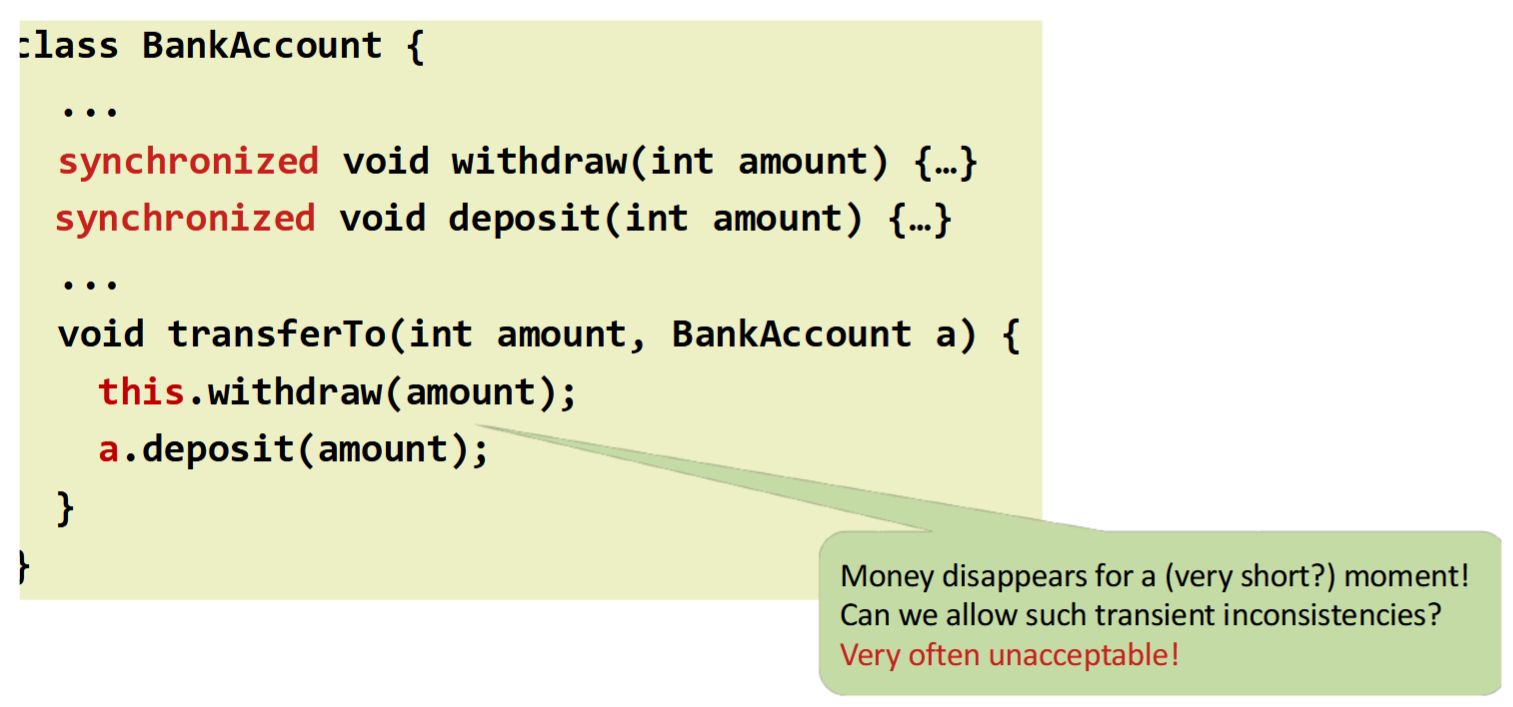
Field-by-field Comparison
| Field |
Before |
After |
| Text |
One way to break the <code>transferTo</code> deadlock is to {{c1::remove the outer <code>synchronized</code> on <code>transferTo</code>}}, leaving only the per-method locks on <code>withdraw</code> and <code>deposit</code>. The trade-off is a {{c2::transient inconsistency: between the withdraw and the deposit, the money is briefly missing from both accounts}}. |
One way to break the <code>transferTo</code> deadlock is to {{c1::remove the outer <code>synchronized</code> on <code>transferTo</code>, leaving only the per-method locks on <code>withdraw</code> and <code>deposit</code>}}.<br><br>The trade-off is a {{c2::transient inconsistency: between the withdraw and the deposit, the money is briefly missing from both accounts}}. |
| Extra |
For financial systems this is usually unacceptable: an external observer (audit, balance read) could see the missing amount. Smaller critical sections are a good move whenever the application can tolerate seeing intermediate states. |
For financial systems this is usually unacceptable: an external observer (audit, balance read) could see the missing amount. Smaller critical sections are a good move whenever the application can tolerate seeing intermediate states.<br><br><img src="paste-622b090b2c0e04672451be52eb56367535f001e8.jpg"> |
Tags:
ETH::2._Semester::PProg::12._Shared_Memory_Concurrency::7._Deadlock_Avoidance
Note 56: ETH::2. Semester::PProg
Deck: ETH::2. Semester::PProg
Note Type: Horvath Cloze
GUID: ]SzQ}B-b0#
modified
Before
Front
ETH::2._Semester::PProg::12._Shared_Memory_Concurrency::5._Locks_with_Atomic_Registers
A common Java bug when implementing Peterson's lock is writing volatile boolean[] flag = new boolean[2];, which makes only the array reference volatile, not its elements. Element accesses then have no volatile semantics. The correct fix is to use AtomicIntegerArray (or AtomicIntegerArray for victim).
Back
ETH::2._Semester::PProg::12._Shared_Memory_Concurrency::5._Locks_with_Atomic_Registers
A common Java bug when implementing Peterson's lock is writing volatile boolean[] flag = new boolean[2];, which makes only the array reference volatile, not its elements. Element accesses then have no volatile semantics. The correct fix is to use AtomicIntegerArray (or AtomicIntegerArray for victim).
The buggy version may appear to work in practice (especially on x86), but provides no JMM guarantees about visibility and ordering of writes to individual array slots. AtomicIntegerArray exposes per-element atomic and volatile-like operations.
After
Front
ETH::2._Semester::PProg::12._Shared_Memory_Concurrency::5._Locks_with_Atomic_Registers
A common Java bug when implementing Peterson's lock is writing
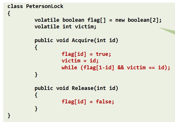
, which makes
only the array reference volatile, not its elements. Element accesses then have no volatile semantics.
The correct fix is to use
AtomicIntegerArray (or AtomicIntegerArray for victim).
Back
ETH::2._Semester::PProg::12._Shared_Memory_Concurrency::5._Locks_with_Atomic_Registers
A common Java bug when implementing Peterson's lock is writing
, which makes
only the array reference volatile, not its elements. Element accesses then have no volatile semantics.
The correct fix is to use
AtomicIntegerArray (or AtomicIntegerArray for victim).
The buggy version may appear to work in practice (especially on x86), but provides no JMM guarantees about visibility and ordering of writes to individual array slots. AtomicIntegerArray exposes per-element atomic and volatile-like operations.
Field-by-field Comparison
| Field |
Before |
After |
| Text |
A common Java bug when implementing Peterson's lock is writing <code>volatile boolean[] flag = new boolean[2];</code>, which makes {{c1::only the array <i>reference</i> volatile, not its <i>elements</i>}}. Element accesses then have no volatile semantics. The correct fix is to use {{c2::<code>AtomicIntegerArray</code> (or <code>AtomicIntegerArray</code> for <code>victim</code>)}}. |
A common Java bug when implementing Peterson's lock is writing <br><code><br><img src="paste-f98c62f8d225881fac276df72497237c0e0339e3.jpg"><br><br></code>, which makes {{c1::only the array <i>reference</i> volatile, not its <i>elements</i>}}. Element accesses then have no volatile semantics. <br><br>The correct fix is to use {{c1::<code>AtomicIntegerArray</code> (or <code>AtomicIntegerArray</code> for <code>victim</code>)}}. |
Tags:
ETH::2._Semester::PProg::12._Shared_Memory_Concurrency::5._Locks_with_Atomic_Registers
Note 57: ETH::2. Semester::PProg
Deck: ETH::2. Semester::PProg
Note Type: Horvath Cloze
GUID: _19oq0$uNl
modified
Before
Front
ETH::2._Semester::PProg::12._Shared_Memory_Concurrency::8._Semaphores
Correct rendezvous implementation with
P_Arrived = Q_Arrived = 0:
| P | Q |
|---|
release(P_Arrived)
acquire(Q_Arrived) | release(Q_Arrived)
acquire(P_Arrived) |
Rule:
signal first ("I am here"), then wait ("are you here too?"). No deadlock is possible because the own
release is already executed before waiting on the other one.
Back
ETH::2._Semester::PProg::12._Shared_Memory_Concurrency::8._Semaphores
Correct rendezvous implementation with
P_Arrived = Q_Arrived = 0:
| P | Q |
|---|
release(P_Arrived)
acquire(Q_Arrived) | release(Q_Arrived)
acquire(P_Arrived) |
Rule:
signal first ("I am here"), then wait ("are you here too?"). No deadlock is possible because the own
release is already executed before waiting on the other one.
Whether P or Q arrives first does not matter: the earlier one waits, the later one triggers both releases before its acquire. Both pass the rendezvous as soon as the second thread arrives.
After
Front
ETH::2._Semester::PProg::12._Shared_Memory_Concurrency::8._Semaphores
Correct rendezvous implementation:
Rule:
Signal first ("I am here"), then wait ("are you here too?").
No deadlock is possible because
the own release is already executed before waiting on the other one.
Back
ETH::2._Semester::PProg::12._Shared_Memory_Concurrency::8._Semaphores
Correct rendezvous implementation:
Rule:
Signal first ("I am here"), then wait ("are you here too?").
No deadlock is possible because
the own release is already executed before waiting on the other one.
Whether P or Q arrives first does not matter: the earlier one waits, the later one triggers both releases before its acquire. Both pass the rendezvous as soon as the second thread arrives.
Field-by-field Comparison
| Field |
Before |
After |
| Text |
Correct rendezvous implementation with <code>P_Arrived = Q_Arrived = 0</code>: <table border="1" cellpadding="4"><tr><th>P</th><th>Q</th></tr><tr><td>{{c1::<code>release(P_Arrived)</code><br><code>acquire(Q_Arrived)</code>}}</td><td>{{c1::<code>release(Q_Arrived)</code><br><code>acquire(P_Arrived)</code>}}</td></tr></table>Rule: {{c2::signal first ("I am here"), then wait ("are you here too?")}}. No deadlock is possible because the own <code>release</code> is already executed before waiting on the other one. |
Correct rendezvous implementation:<br><font face="monospace"><br></font><img src="paste-449fc88e56639a1fbba68957ab236205c15a0780.jpg"><font face="monospace"><br><br></font>Rule: {{c1::Signal first ("I am here"), then wait ("are you here too?")}}. <br>No deadlock is possible because {{c2::the own <code>release</code> is already executed before waiting on the other one}}. |
Tags:
ETH::2._Semester::PProg::12._Shared_Memory_Concurrency::8._Semaphores
Note 58: ETH::2. Semester::PProg
Deck: ETH::2. Semester::PProg
Note Type: Horvath Cloze
GUID: _9&=
modified
Before
Front
ETH::2._Semester::PProg::12._Shared_Memory_Concurrency::7._Deadlock_Avoidance
Two strategies for handling deadlocks: detection (find cycles in the resource graph at runtime; cannot in general be healed because releasing locks usually leaves inconsistent state) and avoidance (statically ensure a cycle can never form). Two standard avoidance techniques are two-phase locking with retry (release everything and restart on conflict; common in databases where transactions can be aborted) and resource ordering (impose a global total order on locks; common in parallel programming where state mutations are not transactional).
Back
ETH::2._Semester::PProg::12._Shared_Memory_Concurrency::7._Deadlock_Avoidance
Two strategies for handling deadlocks: detection (find cycles in the resource graph at runtime; cannot in general be healed because releasing locks usually leaves inconsistent state) and avoidance (statically ensure a cycle can never form). Two standard avoidance techniques are two-phase locking with retry (release everything and restart on conflict; common in databases where transactions can be aborted) and resource ordering (impose a global total order on locks; common in parallel programming where state mutations are not transactional).
Detection is reactive; avoidance is proactive. Avoidance is preferred when consistency requirements rule out the rollback-and-retry approach.
After
Front
ETH::2._Semester::PProg::12._Shared_Memory_Concurrency::7._Deadlock_Avoidance
Two strategies for handling deadlocks:
- Detection (find cycles in the resource graph at runtime; cannot in general be healed because releasing locks usually leaves inconsistent state)
- Avoidance (statically ensure a cycle can never form)
Back
ETH::2._Semester::PProg::12._Shared_Memory_Concurrency::7._Deadlock_Avoidance
Two strategies for handling deadlocks:
- Detection (find cycles in the resource graph at runtime; cannot in general be healed because releasing locks usually leaves inconsistent state)
- Avoidance (statically ensure a cycle can never form)
Detection is reactive; avoidance is proactive. Avoidance is preferred when consistency requirements rule out the rollback-and-retry approach.
Field-by-field Comparison
| Field |
Before |
After |
| Text |
Two strategies for handling deadlocks: {{c1::detection (find cycles in the resource graph at runtime; cannot in general be healed because releasing locks usually leaves inconsistent state)}} and {{c2::avoidance (statically ensure a cycle can never form)}}. Two standard avoidance techniques are {{c3::two-phase locking with retry (release everything and restart on conflict; common in databases where transactions can be aborted)}} and {{c3::resource ordering (impose a global total order on locks; common in parallel programming where state mutations are not transactional)}}. |
Two strategies for handling deadlocks: <br><ol><li>{{c1::Detection (find cycles in the resource graph at runtime; cannot in general be healed because releasing locks usually leaves inconsistent state)}} </li><li>{{c2::Avoidance (statically ensure a cycle can never form)}}</li></ol> |
Tags:
ETH::2._Semester::PProg::12._Shared_Memory_Concurrency::7._Deadlock_Avoidance
Note 59: ETH::2. Semester::PProg
Deck: ETH::2. Semester::PProg
Note Type: Horvath Cloze
GUID: g?{Lm[l$i^
modified
Before
Front
ETH::2._Semester::PProg::12._Shared_Memory_Concurrency::4._Java_Memory_Model
HB consistency: a read sees either the latest write in HB or any other write that is unordered with respect to it in HB.
Consequence: the JMM explicitly allows data races rather than forbidding them.
Back
ETH::2._Semester::PProg::12._Shared_Memory_Concurrency::4._Java_Memory_Model
HB consistency: a read sees either the latest write in HB or any other write that is unordered with respect to it in HB.
Consequence: the JMM explicitly allows data races rather than forbidding them.
Example: in a race a read may observe an "old" value even though a newer write exists, as long as that newer write is not HB-before the read. This is how the typical "impossible" outcomes arise.
After
Front
ETH::2._Semester::PProg::12._Shared_Memory_Concurrency::4._Java_Memory_Model
HB consistency: a read sees either the latest write in HB or any other write that is unordered with respect to it in HB.
Consequence: the JMM explicitly allows data races rather than forbidding them.
Back
ETH::2._Semester::PProg::12._Shared_Memory_Concurrency::4._Java_Memory_Model
HB consistency: a read sees either the latest write in HB or any other write that is unordered with respect to it in HB.
Consequence: the JMM explicitly allows data races rather than forbidding them.
Example: in a race a read may observe an "old" value even though a newer write exists, as long as that newer write is not HB-before the read. This is how the typical "impossible" outcomes arise.
Field-by-field Comparison
| Field |
Before |
After |
| Text |
<i>HB consistency</i>: a read sees either {{c1::the latest write in HB}} or {{c1::any other write that is unordered with respect to it in HB}}. <br><br>Consequence: the JMM {{c2::explicitly allows data races}} rather than forbidding them. |
<i>HB consistency</i>: a read sees either {{c1::the latest write in HB}} or {{c1::any other write that is unordered with respect to it in HB}}. <br><br>Consequence: the JMM {{c2::explicitly allows data races}} rather than {{c2::forbidding them}}. |
Tags:
ETH::2._Semester::PProg::12._Shared_Memory_Concurrency::4._Java_Memory_Model
Note 60: ETH::2. Semester::PProg
Deck: ETH::2. Semester::PProg
Note Type: Horvath Cloze
GUID: iM|cWW?YzD
modified
Before
Front
ETH::2._Semester::PProg::12._Shared_Memory_Concurrency::9._Barriers
Scaling a dot product to 1 million entries on 10 000 threads is impractical with semaphores or locks. It calls for a higher-level abstraction supporting threads in bulk mode (all moving in lock-step). The corresponding programming model is Bulk-Synchronous Parallel (BSP).
Back
ETH::2._Semester::PProg::12._Shared_Memory_Concurrency::9._Barriers
Scaling a dot product to 1 million entries on 10 000 threads is impractical with semaphores or locks. It calls for a higher-level abstraction supporting threads in bulk mode (all moving in lock-step). The corresponding programming model is Bulk-Synchronous Parallel (BSP).
The full BSP model (Valiant, 1990) is more general and supports distributed memory: computation proceeds in supersteps consisting of local computation, communication, and a global barrier. In shared-memory code the barrier is the central building block.
After
Front
ETH::2._Semester::PProg::12._Shared_Memory_Concurrency::9._Barriers
Scaling a dot product to 1 million entries on 10 000 threads is impractical with semaphores or locks. It calls for a higher-level abstraction supporting threads in bulk mode (all moving in lock-step).
The corresponding programming model is Bulk-Synchronous Parallel (BSP).
Back
ETH::2._Semester::PProg::12._Shared_Memory_Concurrency::9._Barriers
Scaling a dot product to 1 million entries on 10 000 threads is impractical with semaphores or locks. It calls for a higher-level abstraction supporting threads in bulk mode (all moving in lock-step).
The corresponding programming model is Bulk-Synchronous Parallel (BSP).
The full BSP model (Valiant, 1990) is more general and supports distributed memory: computation proceeds in supersteps consisting of local computation, communication, and a global barrier. In shared-memory code the barrier is the central building block.
Field-by-field Comparison
| Field |
Before |
After |
| Text |
Scaling a dot product to 1 million entries on 10 000 threads is impractical with semaphores or locks. It calls for a higher-level abstraction supporting {{c1::threads in bulk mode}} (all moving in lock-step). The corresponding programming model is {{c2::Bulk-Synchronous Parallel (BSP)}}. |
Scaling a dot product to 1 million entries on 10 000 threads is impractical with semaphores or locks. It calls for a higher-level abstraction supporting {{c1::threads in bulk mode (all moving in lock-step)}}. <br><br>The corresponding programming model is {{c1::Bulk-Synchronous Parallel (BSP)}}. |
Tags:
ETH::2._Semester::PProg::12._Shared_Memory_Concurrency::9._Barriers
Note 61: ETH::2. Semester::PProg
Deck: ETH::2. Semester::PProg
Note Type: Horvath Cloze
GUID: kU$/VTuynM
modified
Before
Front
ETH::2._Semester::PProg::12._Shared_Memory_Concurrency::7._Deadlock_Avoidance
The historic Java StringBuffer.append(StringBuffer sb) (synchronized append(...){ int len = sb.length(); ... sb.getChars(0, len, value, count); }) has two problems: the lock on sb is not held between sb.length() and sb.getChars(...), so sb can grow or shrink in between (a shrinking sb definitely breaks append) and deadlock potential on crossing calls x.append(y) and y.append(x) on two threads, analogous to the bank-account transfer example.
Back
ETH::2._Semester::PProg::12._Shared_Memory_Concurrency::7._Deadlock_Avoidance
The historic Java StringBuffer.append(StringBuffer sb) (synchronized append(...){ int len = sb.length(); ... sb.getChars(0, len, value, count); }) has two problems: the lock on sb is not held between sb.length() and sb.getChars(...), so sb can grow or shrink in between (a shrinking sb definitely breaks append) and deadlock potential on crossing calls x.append(y) and y.append(x) on two threads, analogous to the bank-account transfer example.
Neither problem is easy to fix without overhead: you do not want a unique id on every StringBuffer, nor a single global lock for all of them. The Java library initially fixed neither (only changed the javadoc) and later split the API into StringBuffer (claimed synchronized) and StringBuilder (not synchronized), leaving clients to avoid such situations with their own protocols.
After
Front
ETH::2._Semester::PProg::12._Shared_Memory_Concurrency::7._Deadlock_Avoidance
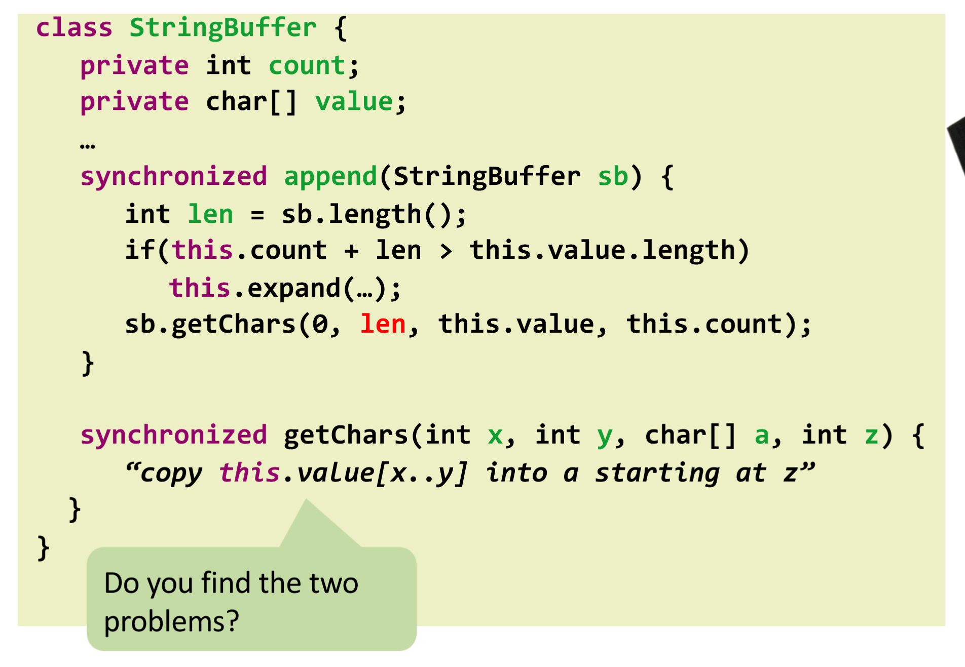
The historic Java
StringBuffer.append has two problems:
- The lock on
sb is not held between sb.length() and sb.getChars(...), so sb can grow or shrink in between (a shrinking sb definitely breaks append). - Deadlock potential on crossing calls
x.append(y) and y.append(x) on two threads, analogous to the bank-account transfer example.
Back
ETH::2._Semester::PProg::12._Shared_Memory_Concurrency::7._Deadlock_Avoidance
The historic Java
StringBuffer.append has two problems:
- The lock on
sb is not held between sb.length() and sb.getChars(...), so sb can grow or shrink in between (a shrinking sb definitely breaks append). - Deadlock potential on crossing calls
x.append(y) and y.append(x) on two threads, analogous to the bank-account transfer example.
Neither problem is easy to fix without overhead: you do not want a unique id on every StringBuffer, nor a single global lock for all of them. The Java library initially fixed neither (only changed the javadoc) and later split the API into StringBuffer (claimed synchronized) and StringBuilder (not synchronized), leaving clients to avoid such situations with their own protocols.
Field-by-field Comparison
| Field |
Before |
After |
| Text |
The historic Java <code>StringBuffer.append(StringBuffer sb)</code> (<code>synchronized append(...){ int len = sb.length(); ... sb.getChars(0, len, value, count); }</code>) has two problems: {{c1::the lock on <code>sb</code> is not held between <code>sb.length()</code> and <code>sb.getChars(...)</code>, so <code>sb</code> can grow or shrink in between (a shrinking <code>sb</code> definitely breaks <code>append</code>)}} and {{c2::deadlock potential on crossing calls <code>x.append(y)</code> and <code>y.append(x)</code> on two threads, analogous to the bank-account transfer example}}. |
<img src="paste-a59c314b7eb5aaea46a960fd7437ced3cb98c6dd.jpg"><br><br>The historic Java <code>StringBuffer.append</code> has two problems: <br><ol><li>{{c1::The lock on <code>sb</code> is not held between <code>sb.length()</code> and <code>sb.getChars(...)</code>, so <code>sb</code> can grow or shrink in between (a shrinking <code>sb</code> definitely breaks <code>append</code>)}}.</li><li>{{c2::Deadlock potential on crossing calls <code>x.append(y)</code> and <code>y.append(x)</code> on two threads, analogous to the bank-account transfer example}}.</li></ol> |
Tags:
ETH::2._Semester::PProg::12._Shared_Memory_Concurrency::7._Deadlock_Avoidance
Note 62: ETH::2. Semester::PProg
Deck: ETH::2. Semester::PProg
Note Type: Horvath Cloze
GUID: mV#=N#**?7
added
Previous
Note did not exist
New Note
Front
ETH::2._Semester::PProg::12._Shared_Memory_Concurrency::7._Deadlock_Avoidance
Two standard avoidance techniques are:
- Two-phase locking with retry (release everything and restart on conflict; common in databases where transactions can be aborted).
- Resource ordering (impose a global total order on locks; common in parallel programming where state mutations are not transactional).
Back
ETH::2._Semester::PProg::12._Shared_Memory_Concurrency::7._Deadlock_Avoidance
Two standard avoidance techniques are:
- Two-phase locking with retry (release everything and restart on conflict; common in databases where transactions can be aborted).
- Resource ordering (impose a global total order on locks; common in parallel programming where state mutations are not transactional).
Field-by-field Comparison
| Field |
Before |
After |
| Text |
|
Two standard avoidance techniques are:<br><ol><li>{{c1::Two-phase locking with retry (release everything and restart on conflict; common in databases where transactions can be aborted)}}.</li><li>{{c2::Resource ordering (impose a global total order on locks; common in parallel programming where state mutations are not transactional)}}.</li></ol> |
Tags:
ETH::2._Semester::PProg::12._Shared_Memory_Concurrency::7._Deadlock_Avoidance
Note 63: ETH::2. Semester::PProg
Deck: ETH::2. Semester::PProg
Note Type: Horvath Cloze
GUID: p)%lBpQ>Q<
modified
Before
Front
ETH::2._Semester::PProg::12._Shared_Memory_Concurrency::6._Locks_with_Atomic_Operations
Three common families of hardware atomic instructions: Test-And-Set (TAS) - e.g. m68k TSL; Compare-And-Swap (CAS) - e.g. x86 LOCK CMPXCHG, SPARC CASA; Load-Linked / Store-Conditional - e.g. ARM LDREX/STREX, MIPS / POWER / RISC-V LL/SC. They are typically 10-100x slower than plain reads / writes.
Back
ETH::2._Semester::PProg::12._Shared_Memory_Concurrency::6._Locks_with_Atomic_Operations
Three common families of hardware atomic instructions: Test-And-Set (TAS) - e.g. m68k TSL; Compare-And-Swap (CAS) - e.g. x86 LOCK CMPXCHG, SPARC CASA; Load-Linked / Store-Conditional - e.g. ARM LDREX/STREX, MIPS / POWER / RISC-V LL/SC. They are typically 10-100x slower than plain reads / writes.
These primitives are needed because plain atomic registers cannot break the \(\Omega(n)\) space lower bound for \(n\)-thread mutex (Burns-Lynch). They also enable lock-free data structures.
After
Front
ETH::2._Semester::PProg::12._Shared_Memory_Concurrency::6._Locks_with_Atomic_Operations
Three common families of hardware atomic instructions:
- Test-And-Set (TAS) - e.g. m68k
TSL - Compare-And-Swap (CAS) - e.g. x86
LOCK CMPXCHG, SPARC CASA - Load-Linked / Store-Conditional - e.g. ARM
LDREX/STREX, MIPS / POWER / RISC-V LL/SC. They are typically 10-100x slower than plain reads / writes.
Back
ETH::2._Semester::PProg::12._Shared_Memory_Concurrency::6._Locks_with_Atomic_Operations
Three common families of hardware atomic instructions:
- Test-And-Set (TAS) - e.g. m68k
TSL - Compare-And-Swap (CAS) - e.g. x86
LOCK CMPXCHG, SPARC CASA - Load-Linked / Store-Conditional - e.g. ARM
LDREX/STREX, MIPS / POWER / RISC-V LL/SC. They are typically 10-100x slower than plain reads / writes.
These primitives are needed because plain atomic registers cannot break the \(\Omega(n)\) space lower bound for \(n\)-thread mutex (Burns-Lynch). They also enable lock-free data structures.
Field-by-field Comparison
| Field |
Before |
After |
| Text |
Three common families of hardware atomic instructions: {{c1::Test-And-Set (TAS)}} - e.g. m68k <code>TSL</code>; {{c2::Compare-And-Swap (CAS)}} - e.g. x86 <code>LOCK CMPXCHG</code>, SPARC <code>CASA</code>; {{c3::Load-Linked / Store-Conditional}} - e.g. ARM <code>LDREX/STREX</code>, MIPS / POWER / RISC-V <code>LL/SC</code>. They are typically {{c4::10-100x slower than plain reads / writes}}. |
Three common families of hardware atomic instructions: <br><ol><li>{{c1::Test-And-Set (TAS)}} - e.g. m68k <code>TSL</code></li><li>{{c2::Compare-And-Swap (CAS)}} - e.g. x86 <code>LOCK CMPXCHG</code>, SPARC <code>CASA</code></li><li>{{c3::Load-Linked / Store-Conditional}} - e.g. ARM <code>LDREX/STREX</code>, MIPS / POWER / RISC-V <code>LL/SC</code>. They are typically 10-100x slower than plain reads / writes.</li></ol> |
Tags:
ETH::2._Semester::PProg::12._Shared_Memory_Concurrency::6._Locks_with_Atomic_Operations
Note 64: ETH::2. Semester::PProg
Deck: ETH::2. Semester::PProg
Note Type: Horvath Cloze
GUID: qzA@de.%OP
modified
Before
Front
ETH::2._Semester::PProg::12._Shared_Memory_Concurrency::5._Locks_with_Atomic_Registers
The Filter Lock satisfies mutual exclusion, deadlock freedom, and starvation freedom, but it is not first-come-first-served: a thread that finished its doorway later may overtake one that finished earlier.
Back
ETH::2._Semester::PProg::12._Shared_Memory_Concurrency::5._Locks_with_Atomic_Registers
The Filter Lock satisfies mutual exclusion, deadlock freedom, and starvation freedom, but it is not first-come-first-served: a thread that finished its doorway later may overtake one that finished earlier.
Reason: there is no global ticket; progress depends on the level/victim arrays, which are updated continuously. A thread that arrives later can become "victim" at a high level after another thread already passed that level. Bakery is the canonical lock that fixes this.
After
Front
ETH::2._Semester::PProg::12._Shared_Memory_Concurrency::5._Locks_with_Atomic_Registers
The Filter Lock satisfies mutual exclusion, deadlock freedom, and starvation freedom, but it is not first-come-first-served:
A thread that finished its doorway later may overtake one that finished earlier.
Back
ETH::2._Semester::PProg::12._Shared_Memory_Concurrency::5._Locks_with_Atomic_Registers
The Filter Lock satisfies mutual exclusion, deadlock freedom, and starvation freedom, but it is not first-come-first-served:
A thread that finished its doorway later may overtake one that finished earlier.
Reason: There is no global ticket; progress depends on the level/victim arrays, which are updated continuously. A thread that arrives later can become "victim" at a high level after another thread already passed that level. Bakery is the canonical lock that fixes this.
Field-by-field Comparison
| Field |
Before |
After |
| Text |
The Filter Lock satisfies {{c1::mutual exclusion, deadlock freedom, and starvation freedom}}, but it is {{c2::not first-come-first-served}}: a thread that finished its doorway later may overtake one that finished earlier. |
The Filter Lock satisfies {{c1::mutual exclusion, deadlock freedom, and starvation freedom}}, but it is not {{c2::first-come-first-served: <br>A thread that finished its doorway later may overtake one that finished earlier}}. |
| Extra |
Reason: there is no global ticket; progress depends on the level/<code>victim</code> arrays, which are updated continuously. A thread that arrives later can become "victim" at a high level after another thread already passed that level. Bakery is the canonical lock that fixes this. |
Reason: There is no global ticket; progress depends on the level/<code>victim</code> arrays, which are updated continuously. A thread that arrives later can become "victim" at a high level after another thread already passed that level. Bakery is the canonical lock that fixes this. |
Tags:
ETH::2._Semester::PProg::12._Shared_Memory_Concurrency::5._Locks_with_Atomic_Registers
Note 65: ETH::2. Semester::PProg
Deck: ETH::2. Semester::PProg
Note Type: Horvath Cloze
GUID: x$osz_e?7R
modified
Before
Front
ETH::2._Semester::PProg::12._Shared_Memory_Concurrency::8._Semaphores
Wrong rendezvous implementation with
P_Arrived = Q_Arrived = 0:
| P | Q |
|---|
acquire(Q_Arrived)
release(P_Arrived) | acquire(P_Arrived)
release(Q_Arrived) |
Problem:
deadlock, because
both threads acquire before anyone has released: P needs Q_Arrived (held by Q), Q needs P_Arrived (held by P): a circular wait.
Back
ETH::2._Semester::PProg::12._Shared_Memory_Concurrency::8._Semaphores
Wrong rendezvous implementation with
P_Arrived = Q_Arrived = 0:
| P | Q |
|---|
acquire(Q_Arrived)
release(P_Arrived) | acquire(P_Arrived)
release(Q_Arrived) |
Problem:
deadlock, because
both threads acquire before anyone has released: P needs Q_Arrived (held by Q), Q needs P_Arrived (held by P): a circular wait.
Lesson: in a rendezvous, always signal first, then wait. Otherwise a classic hold-and-wait cycle forms because neither thread ever reaches its release.
After
Front
ETH::2._Semester::PProg::12._Shared_Memory_Concurrency::8._Semaphores
Wrong rendezvous implementation:
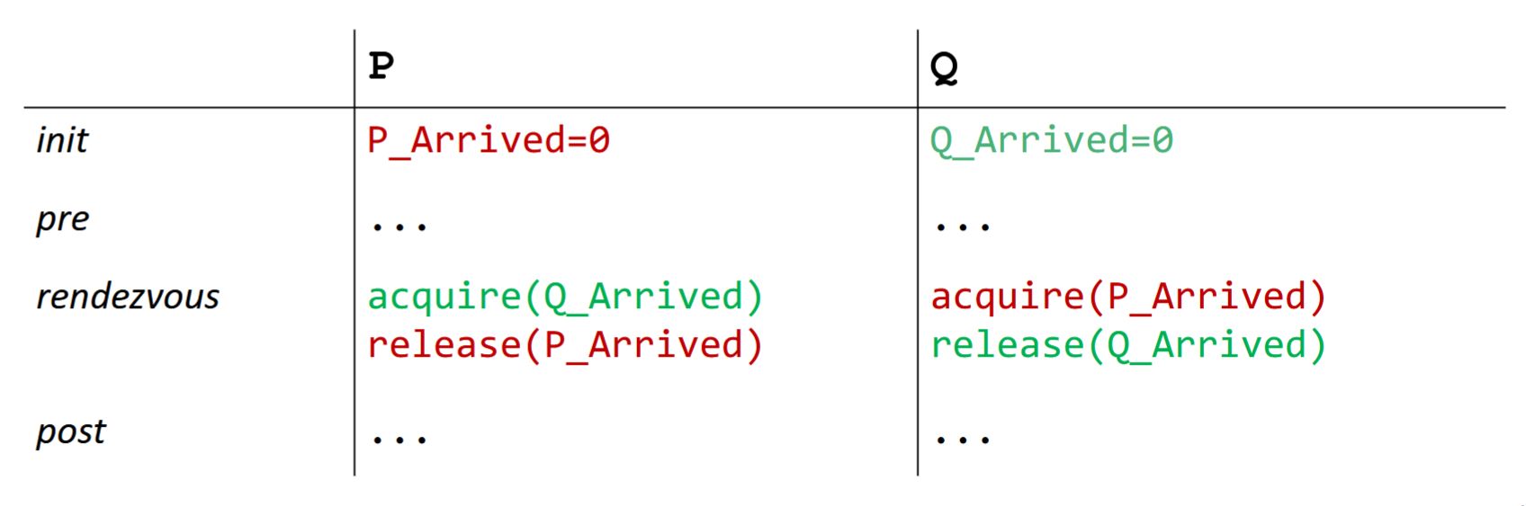
Problem:
deadlock, because
both threads acquire before anyone has released: P needs Q_Arrived (held by Q), Q needs P_Arrived (held by P): a circular wait.
Back
ETH::2._Semester::PProg::12._Shared_Memory_Concurrency::8._Semaphores
Wrong rendezvous implementation:
Problem:
deadlock, because
both threads acquire before anyone has released: P needs Q_Arrived (held by Q), Q needs P_Arrived (held by P): a circular wait.
Lesson: in a rendezvous, always
signal first, then wait. Otherwise a classic hold-and-wait cycle forms because neither thread ever reaches its
release.
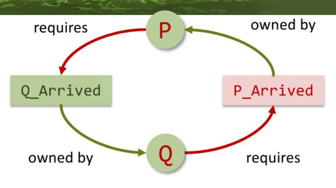
Field-by-field Comparison
| Field |
Before |
After |
| Text |
Wrong rendezvous implementation with <code>P_Arrived = Q_Arrived = 0</code>: <table border="1" cellpadding="4"><tr><th>P</th><th>Q</th></tr><tr><td><code>acquire(Q_Arrived)</code><br><code>release(P_Arrived)</code></td><td><code>acquire(P_Arrived)</code><br><code>release(Q_Arrived)</code></td></tr></table>Problem: {{c1::deadlock}}, because {{c2::both threads acquire before anyone has released: <code>P</code> needs <code>Q_Arrived</code> (held by Q), <code>Q</code> needs <code>P_Arrived</code> (held by P): a circular wait}}. |
Wrong rendezvous implementation:<br><br><img src="paste-ba3515ab9b41f03da81e714beffc8e3b959aed12.jpg"><br><br>Problem: {{c1::deadlock}}, because {{c1::both threads acquire before anyone has released: <code>P</code> needs <code>Q_Arrived</code> (held by Q), <code>Q</code> needs <code>P_Arrived</code> (held by P): a circular wait}}. |
| Extra |
Lesson: in a rendezvous, always <em>signal first, then wait</em>. Otherwise a classic hold-and-wait cycle forms because neither thread ever reaches its <code>release</code>. |
Lesson: in a rendezvous, always <em>signal first, then wait</em>. Otherwise a classic hold-and-wait cycle forms because neither thread ever reaches its <code>release</code>.<br><br><img src="paste-b89b81ae16962c5a2cb87af1f107795940c8a81e.jpg"> |
Tags:
ETH::2._Semester::PProg::12._Shared_Memory_Concurrency::8._Semaphores
Note 66: ETH::2. Semester::PProg
Deck: ETH::2. Semester::PProg
Note Type: Horvath Cloze
GUID: y4X/i|x>Tz
modified
Before
Front
ETH::2._Semester::PProg::12._Shared_Memory_Concurrency::9._Barriers
Wrong barrier implementation with semaphore barrier = 0 and shared variable count = 0: each thread does count++; if (count == n) release(barrier); acquire(barrier);. Problems: race condition on count++ (no mutex) and deadlock, because release is called only once but \(n\) threads acquire: after the first acquire the semaphore is back to 0, so all others wait forever.
Back
ETH::2._Semester::PProg::12._Shared_Memory_Concurrency::9._Barriers
Wrong barrier implementation with semaphore barrier = 0 and shared variable count = 0: each thread does count++; if (count == n) release(barrier); acquire(barrier);. Problems: race condition on count++ (no mutex) and deadlock, because release is called only once but \(n\) threads acquire: after the first acquire the semaphore is back to 0, so all others wait forever.
Violated invariants: "count gives the number of processes that have passed the barrier" and "once all processes have reached the barrier, all waiting processes can continue". Both must be fixed separately: the race with a mutex, the deadlock with a turnstile.
After
Front
ETH::2._Semester::PProg::12._Shared_Memory_Concurrency::9._Barriers
Wrong barrier implementation with semaphore:
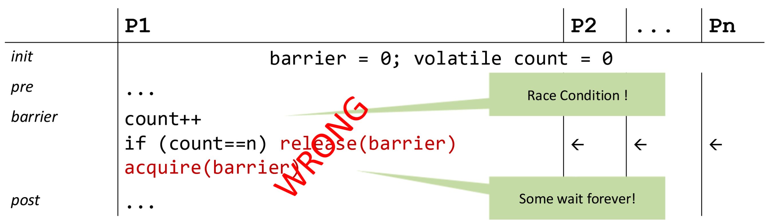
Problems:
race condition on count++ (no mutex) and
deadlock, because release is called only once but \(n\) threads acquire: after the first acquire the semaphore is back to 0, so all others wait forever.
Back
ETH::2._Semester::PProg::12._Shared_Memory_Concurrency::9._Barriers
Wrong barrier implementation with semaphore:
Problems:
race condition on count++ (no mutex) and
deadlock, because release is called only once but \(n\) threads acquire: after the first acquire the semaphore is back to 0, so all others wait forever.
Violated invariants: "count gives the number of processes that have passed the barrier" and "once all processes have reached the barrier, all waiting processes can continue". Both must be fixed separately: the race with a mutex, the deadlock with a turnstile.
Field-by-field Comparison
| Field |
Before |
After |
| Text |
Wrong barrier implementation with semaphore <code>barrier = 0</code> and shared variable <code>count = 0</code>: each thread does <code>count++; if (count == n) release(barrier); acquire(barrier);</code>. Problems: {{c1::race condition on <code>count++</code> (no mutex)}} and {{c2::deadlock, because <code>release</code> is called only once but \(n\) threads <code>acquire</code>: after the first <code>acquire</code> the semaphore is back to 0, so all others wait forever}}. |
Wrong barrier implementation with semaphore:<br><br><img src="paste-5871ecc6e94ff43962d684c318c6547f462564d6.jpg"><br><br>Problems: {{c1::race condition on <code>count++</code> (no mutex)}} and {{c1::deadlock, because <code>release</code> is called only once but \(n\) threads <code>acquire</code>: after the first <code>acquire</code> the semaphore is back to 0, so all others wait forever}}. |
Tags:
ETH::2._Semester::PProg::12._Shared_Memory_Concurrency::9._Barriers