Anki Deck Changes

Note 1: ETH::A&D

Deck: ETH::A&D
Note Type: Algorithms
GUID: DeJ!2ph{Al

modified

Before

Front

Runtime of Johnson's Algorithm?

Back

Runtime of Johnson's Algorithm?

\(O(|V| \cdot (|V| + |E|) \log |V|)\) (running dijkstra's n times, but allows negatives)

After

Front

Runtime of Johnson's Algorithm?

Back

Runtime of Johnson's Algorithm?

\(O(|V| \cdot (|V| + |E|) \log |V|)\) (running dijkstra's n times, but allows negatives)

Field-by-field Comparison

Field	Before	After
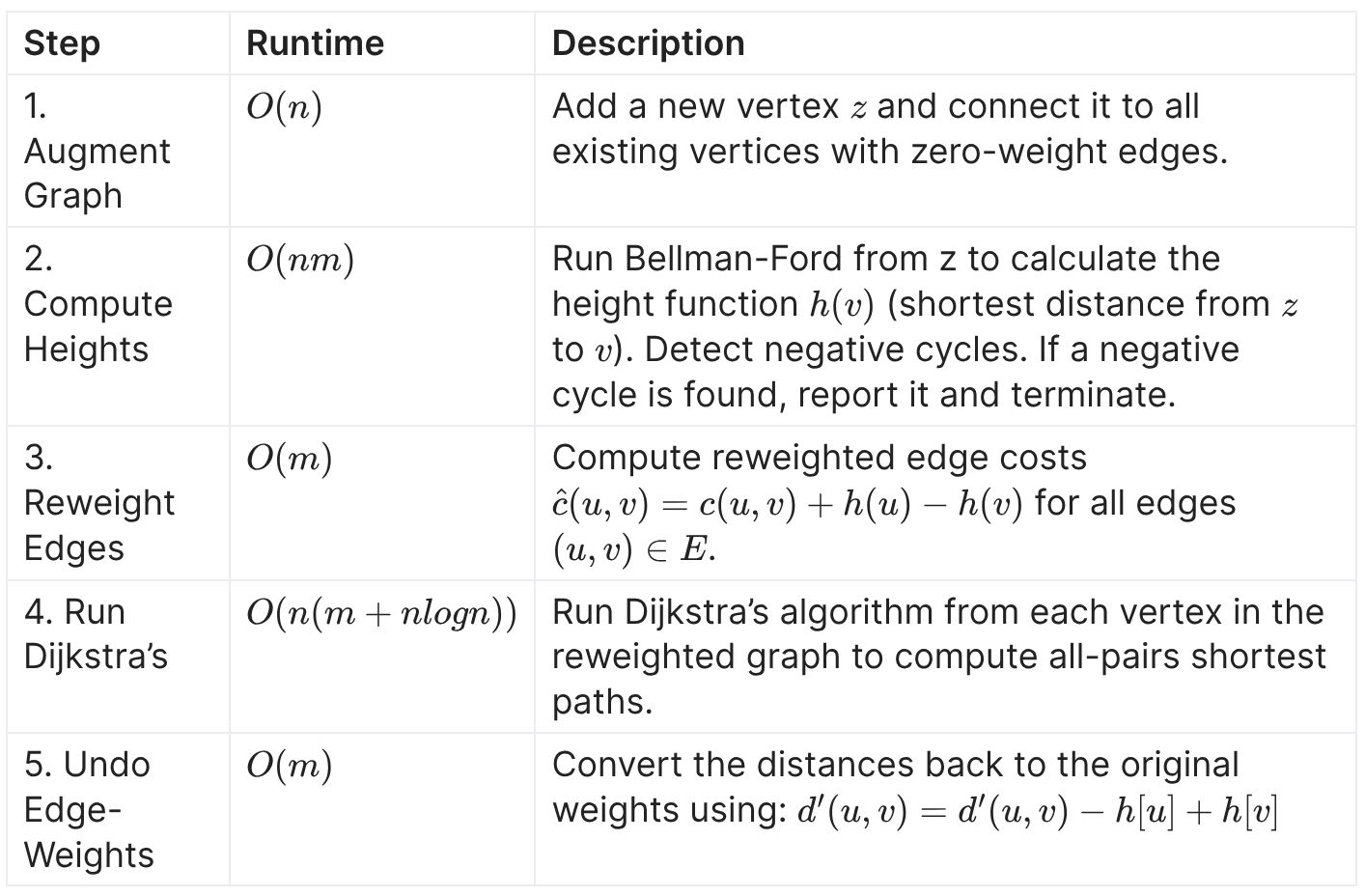
Approach	<ol><li><b>Add a New Vertex:</b><ul><li>Add a new vertex s to the graph and connect it to all vertices with zero-weight edges. </li> </ul></li><li><b>Run Bellman-Ford</b>:<ul><li>Use the Bellman-Ford algorithm starting from s to compute the shortest distance h[v] from s to each vertex v.</li><li>If a negative-weight cycle is detected, stop.</li></ul></li><li><b>Reweight Edges</b>: <ul><li>For each edge u → v with weight w(u, v), reweight it as: w′(u, v) = w(u, v) + h[u] − h[v]</li><li>This ensures all edge weights are non-negative.</li> </ul> </li><li><b>Run Dijkstra’s Algorithm:</b><ul><li>For each vertex v, use Dijkstra’s algorithm to compute the shortest paths to all other vertices.</li> </ul></li><li><b>Adjust Back</b>:<ul><li>Convert the distances back to the original weights using: d′(u, v) = d′(u, v) − h[u] + h[v]</li> </ul></li><li><b>End:</b></li><ul><li>The resulting shortest path distances between all pairs of vertices are valid.</li></ul></ol><div>The overall higher cost allows us to run pre-computation steps like B-F for "free"</div>	<ol><li><b>Add a New Vertex:</b><ul><li>Add a new vertex s to the graph and connect it to all vertices with zero-weight edges. </li> </ul></li><li><b>Run Bellman-Ford</b>:<ul><li>Use the Bellman-Ford algorithm starting from s to compute the shortest distance h[v] from s to each vertex v.</li><li>If a negative-weight cycle is detected, stop.</li></ul></li><li><b>Reweight Edges</b>: <ul><li>For each edge u → v with weight w(u, v), reweight it as: w′(u, v) = w(u, v) + h[u] − h[v]</li><li>This ensures all edge weights are non-negative.</li> </ul> </li><li><b>Run Dijkstra’s Algorithm:</b><ul><li>For each vertex v, use Dijkstra’s algorithm to compute the shortest paths to all other vertices.</li> </ul></li><li><b>Adjust Back</b>:<ul><li>Convert the distances back to the original weights using: d′(u, v) = d′(u, v) − h[u] + h[v]</li> </ul></li><li><b>End:</b></li><ul><li>The resulting shortest path distances between all pairs of vertices are valid.</li></ul></ol><div>The overall higher cost allows us to run pre-computation steps like Bellman-Ford for "free".</div>

Tags: ETH::1._Semester::A&D::12._All-Pair_Shortest_Paths::2._Johnson's_Algorithm

Note 2: ETH::A&D

Deck: ETH::A&D
Note Type: Horvath Cloze
GUID: hsaD+h{~n8

modified

Before

Front

Reweighting in Johnson's algorithm:

We add a vertex \(s\) and add a 0 cost edge from it to all vertices.
We then run B-F which determines the height of each vertex by the d[v] from start vertex \(s\)

Back

Reweighting in Johnson's algorithm:

We add a vertex \(s\) and add a 0 cost edge from it to all vertices.
We then run B-F which determines the height of each vertex by the d[v] from start vertex \(s\)

After

Front

Reweighting in Johnson's algorithm:

We add a vertex \(s\) and add a 0 cost edge from it to all vertices.
We then run Bellman-Ford which determines the height of each vertex by the d[v] from start vertex \(s\)

Back

Reweighting in Johnson's algorithm:

We add a vertex \(s\) and add a 0 cost edge from it to all vertices.
We then run Bellman-Ford which determines the height of each vertex by the d[v] from start vertex \(s\)

Field-by-field Comparison

Field	Before	After
Text	Reweighting in Johnson's algorithm:<br><ol><li>We {{c1::add a vertex \(s\)}} and {{c1::add a 0 cost edge from it to all vertices}}.</li><li>We then {{c2::run B-F which determines the height of each vertex by the d[v] from start vertex \(s\)}} </li></ol>	Reweighting in Johnson's algorithm:<br><ol><li>We {{c1::add a vertex \(s\)}} and {{c1::add a 0 cost edge from it to all vertices}}.</li><li>We then {{c2::run Bellman-Ford which determines the height of each vertex by the d[v] from start vertex \(s\)}} </li></ol>

Tags: ETH::1._Semester::A&D::12._All-Pair_Shortest_Paths::2._Johnson's_Algorithm

Note 3: ETH::LinAlg

Deck: ETH::LinAlg
Note Type: Horvath Cloze
GUID: G9![k&wZRU

modified

Before

Front

Given a symmetric matrix \(A \in \mathbb{R}^{n \times n}\) the Rayleigh Quotient defined for \(x \in \mathbb{R}^n \setminus {0}\), as \[ R(x) = {{c1::\frac{x^\top Ax}{x^\top x} }}\]attains it’s

maximum at \(R(v_{\text{max) = \lambda_{\text{max}}\)}}
minimum at \(R(v_{\text{min) = \lambda_{\text{min}}\)}}

where \(\lambda_{\text{max\) and \(\lambda_{\text{min}}\) are respectively the largest and smallest eigenvalues of \(A\) and \(v_{\text{max}}\) and \(v_{\text{min}}\) their associated eigenvectors}}.

Back

Given a symmetric matrix \(A \in \mathbb{R}^{n \times n}\) the Rayleigh Quotient defined for \(x \in \mathbb{R}^n \setminus {0}\), as \[ R(x) = {{c1::\frac{x^\top Ax}{x^\top x} }}\]attains it’s

maximum at \(R(v_{\text{max) = \lambda_{\text{max}}\)}}
minimum at \(R(v_{\text{min) = \lambda_{\text{min}}\)}}

where \(\lambda_{\text{max\) and \(\lambda_{\text{min}}\) are respectively the largest and smallest eigenvalues of \(A\) and \(v_{\text{max}}\) and \(v_{\text{min}}\) their associated eigenvectors}}.

After

Front

Given a symmetric matrix \(A \in \mathbb{R}^{n \times n}\) the Rayleigh Quotient defined for \(x \in \mathbb{R}^n \setminus {0}\), as \[ R(x) = {{c1::\frac{x^\top Ax}{x^\top x} }}\]attains it’s

maximum at {{c2::\(R(v_{\text{max} }) = \lambda_{\text{max} }\)}}
minimum at {{c2::\(R(v_{\text{min} }) = \lambda_{\text{min} } \)}}

where {{c2::\(\lambda_{\text{max} }\) and \(\lambda_{\text{min} }\) are respectively the largest and smallest eigenvalues of \(A\) and \(v_{\text{max} }\) and \(v_{\text{min} }\) their associated eigenvectors}}.

Back

Given a symmetric matrix \(A \in \mathbb{R}^{n \times n}\) the Rayleigh Quotient defined for \(x \in \mathbb{R}^n \setminus {0}\), as \[ R(x) = {{c1::\frac{x^\top Ax}{x^\top x} }}\]attains it’s

maximum at {{c2::\(R(v_{\text{max} }) = \lambda_{\text{max} }\)}}
minimum at {{c2::\(R(v_{\text{min} }) = \lambda_{\text{min} } \)}}

Field-by-field Comparison

Field	Before	After
Text	<div>Given a symmetric matrix \(A \in \mathbb{R}^{n \times n}\) the Rayleigh Quotient defined for \(x \in \mathbb{R}^n \setminus {0}\), as \[ R(x) = {{c1::\frac{x^\top Ax}{x^\top x} }}\]attains it’s</div><div><ul><li>~~{{c2::~~maximum at \(R(v_{\text{max}}) = \lambda_{\text{max}}\)}}</li><li>~~{{c2::~~minimum at \(R(v_{\text{min}}) = \lambda_{\text{min}}\)}}</li></ul><div>where {{c2::\(\lambda_{\text{max}}\) and \(\lambda_{\text{min}}\) are respectively the largest and smallest eigenvalues of \(A\) and \(v_{\text{max}}\) and \(v_{\text{min}}\) their associated eigenvectors}}.</div></div><blockquote><ul> </ul></blockquote>	<div>Given a symmetric matrix \(A \in \mathbb{R}^{n \times n}\) the Rayleigh Quotient defined for \(x \in \mathbb{R}^n \setminus {0}\), as \[ R(x) = {{c1::\frac{x^\top Ax}{x^\top x} }}\]attains it’s</div><div><ul><li>maximum at {{c2::\(R(v_{\text{max} }) = \lambda_{\text{max} }\)}}</li><li>minimum at {{c2::\(R(v_{\text{min} }) = \lambda_{\text{min} } \)}}</li></ul><div>where {{c2::\(\lambda_{\text{max} }\) and \(\lambda_{\text{min} }\) are respectively the largest and smallest eigenvalues of \(A\) and \(v_{\text{max} }\) and \(v_{\text{min} }\) their associated eigenvectors}}.</div></div><blockquote><ul> </ul></blockquote>

Tags: ETH::1._Semester::LinAlg::9._Diagonalisable_Matrices_and_the_SVD::2._Symmetric_Matrices_and_the_Spectral_Theorem::1._Rayleigh_Quotient

Note 4: ETH::LinAlg

Deck: ETH::LinAlg
Note Type: Horvath Cloze
GUID: M;:>m2mzC#

modified

Before

Front

Let \(A \in \mathbb{R}^{m \times n}\). Then \(N(A) = N(A^\top A)\). Proof Included

Back

Let \(A \in \mathbb{R}^{m \times n}\). Then \(N(A) = N(A^\top A)\). Proof Included

\(N(A) = N(A^\top A)\) holds because:

if \(x \in N(A)\) then \(Ax = 0 \implies A^\top Ax = A \cdot 0 \implies A^\top A x = 0\).
if \(x \in N(A^\top A)\) then \(A^\top A x = 0\), which means \[ 0 = x^\top 0 = x^\top A^\top Ax = (Ax)^\top(Ax) = ||Ax||^2 \implies Ax = 0 \]

After

Front

Let \(A \in \mathbb{R}^{m \times n}\). Then \(N(A) = {{c1::N(A^\top A)::\text{another nullspace} }}\). Proof Included

Back

Let \(A \in \mathbb{R}^{m \times n}\). Then \(N(A) = {{c1::N(A^\top A)::\text{another nullspace} }}\). Proof Included

\(N(A) = N(A^\top A)\) holds because:

if \(x \in N(A)\) then \(Ax = 0 \implies A^\top Ax = A \cdot 0 \implies A^\top A x = 0\).
if \(x \in N(A^\top A)\) then \(A^\top A x = 0\), which means \[ 0 = x^\top 0 = x^\top A^\top Ax = (Ax)^\top(Ax) = ||Ax||^2 \implies Ax = 0 \]

Field-by-field Comparison

Field	Before	After
Text	Let \(A \in \mathbb{R}^{m \times n}\). Then \(N(A) = {{c1::N(A^\top A)}}\). <i>Proof Included</i>	Let \(A \in \mathbb{R}^{m \times n}\). Then \(N(A) = {{c1::N(A^\top A)::\text{another nullspace} }}\). <i>Proof Included</i>

Tags: ETH::1._Semester::LinAlg::5._Orthogonality_and_Projections::1._Orthogonality

Note 5: ETH::LinAlg

Deck: ETH::LinAlg
Note Type: Horvath Cloze
GUID: OYJ^1jnB1-

modified

Before

Front

Real antisymmetric matrices always have imaginary (or zero) eigenvalues.

Back

Real antisymmetric matrices always have imaginary (or zero) eigenvalues.

After

Front

Real antisymmetric matrices always have imaginary (or zero) eigenvalues.

Back

Real antisymmetric matrices always have imaginary (or zero) eigenvalues.

Antisymmetric means \(A^T=-A\).

Field-by-field Comparison

Field	Before	After
Extra		Antisymmetric means \(A^T=-A\).

Tags: ETH::1._Semester::LinAlg::8._Eigenvalues_and_Eigenvectors::5._Extra

Note 6: ETH::LinAlg

Deck: ETH::LinAlg
Note Type: Horvath Cloze
GUID: Pa)fnn7&WJ

modified

Before

Front

\(A \in \mathbb{R}^{n \times n}\) arbitrary non-symmetric has rank \(n - \dim(N(A))\) so it's \(n\) minus the geometric multiplicity of \(\lambda = 0\) .

Back

\(A \in \mathbb{R}^{n \times n}\) arbitrary non-symmetric has rank \(n - \dim(N(A))\) so it's \(n\) minus the geometric multiplicity of \(\lambda = 0\) .

After

Front

\(A \in \mathbb{R}^{n \times n}\) arbitrary non-symmetric has rank \(n - \dim(N(A))\) so it's \(n\) minus the geometric multiplicity of \(\lambda = 0\) .

Back

\(A \in \mathbb{R}^{n \times n}\) arbitrary non-symmetric has rank \(n - \dim(N(A))\) so it's \(n\) minus the geometric multiplicity of \(\lambda = 0\) .

Field-by-field Comparison

Field	Before	After
Text	\(A \in \mathbb{R}^{n \times n}\) arbitrary non-symmetric has rank {{c1::  \(n - \dim(N(A))\) so it's \(n\) minus the geometric multiplicity of \(\lambda = 0\) :: in terms of multiplicities}}.	\(A \in \mathbb{R}^{n \times n}\) arbitrary non-symmetric has rank {{c1:: \(n - \dim(N(A))\) so it's \(n\) minus the geometric multiplicity of \(\lambda = 0\) ::in terms of multiplicities}}.

Tags: ETH::1._Semester::LinAlg::9._Diagonalisable_Matrices_and_the_SVD::2._Symmetric_Matrices_and_the_Spectral_Theorem

Note 7: ETH::LinAlg

Deck: ETH::LinAlg
Note Type: Horvath Cloze
GUID: d9#?3c)V#_

modified

Before

Front

Let \(A \in \mathbb{R}^{n \times n}\) be a symmetric matrix and \(\lambda \in \mathbb{C}\) be an eigenvalue of \(A\), then {{c1::\(\lambda \in \mathbb{R}\):: property of the EW}}. Proof Included

Back

Let \(A \in \mathbb{R}^{n \times n}\) be a symmetric matrix and \(\lambda \in \mathbb{C}\) be an eigenvalue of \(A\), then {{c1::\(\lambda \in \mathbb{R}\):: property of the EW}}. Proof Included

Proof \(v \in \mathbb{C}^n\) be EV of \(\lambda\). Thus we have \(Av = \lambda v\). Since \(A\) is symmetric we have \(A^ = A\). \[\begin{align} \overline{\lambda}||v||^2 &= \overline{\lambda} v^*v \\ &= (\lambda v)^*v \\ &= (Av)^*v = v^*A^*v \\ &= v^* Av \text{ (uses } A^* = A \text{) } \\ &= v^*\lambda v \\ &= \lambda ||v||^2 \end{align}\]Since \(v \neq 0\), then \(||v|| \neq 0\) and so \(\lambda = \overline{\lambda}\) thus \(\lambda \in \mathbb{R}\).

After

Front

Let \(A \in \mathbb{R}^{n \times n}\) be a symmetric matrix and \(\lambda \in \mathbb{C}\) be an eigenvalue of \(A\), then {{c1::\(\lambda \in \mathbb{R}\)::property of the EW}}. Proof Included

Back

Let \(A \in \mathbb{R}^{n \times n}\) be a symmetric matrix and \(\lambda \in \mathbb{C}\) be an eigenvalue of \(A\), then {{c1::\(\lambda \in \mathbb{R}\)::property of the EW}}. Proof Included

Field-by-field Comparison

Field	Before	After
Text	Let \(A \in \mathbb{R}^{n \times n}\) be a symmetric matrix and \(\lambda \in \mathbb{C}\) be an eigenvalue of \(A\), then {{c1::\(\lambda \in \mathbb{R}\):: property of the EW}}. <i>Proof Included</i>	Let \(A \in \mathbb{R}^{n \times n}\) be a symmetric matrix and \(\lambda \in \mathbb{C}\) be an eigenvalue of \(A\), then {{c1::\(\lambda \in \mathbb{R}\)::property of the EW}}. <i>Proof Included</i>

Tags: ETH::1._Semester::LinAlg::9._Diagonalisable_Matrices_and_the_SVD::2._Symmetric_Matrices_and_the_Spectral_Theorem

Note 8: ETH::LinAlg

Deck: ETH::LinAlg
Note Type: Horvath Cloze
GUID: dZ)aTr>2eb

modified

Before

Front

Given a real matrix \(A \in \mathbb{R}^{n \times n}\), the non-zero eigenvalues of \(A^\top A\) are the same ones of \(AA^\top\). Proof Included

Back

Given a real matrix \(A \in \mathbb{R}^{n \times n}\), the non-zero eigenvalues of \(A^\top A\) are the same ones of \(AA^\top\). Proof Included

Shared EWs: For \((A\top A)v_k = \lambda_k v_k\) we get \(AA^\top A v_k = \lambda_k Av_k\) and thus \(Av_k\) EV and \(\lambda_k\) is an EW of \(AA^\top\).

Orthogonality: For \(j \neq k\) we have \((Av_j)^\top (Av_k) = v_j^\top A^\top Av_k = v_j^\top \lambda_k v_k = \lambda_k v_j^\top v_k = 0\)

After

Front

Given a real matrix \(A \in \mathbb{R}^{n \times n}\), the non-zero eigenvalues of \(A^\top A\) are the same ones of \(AA^\top\). Proof Included

Back

Given a real matrix \(A \in \mathbb{R}^{n \times n}\), the non-zero eigenvalues of \(A^\top A\) are the same ones of \(AA^\top\). Proof Included

Shared EWs: For \((A^\top A)v_k = \lambda_k v_k\) we get \(AA^\top A v_k = \lambda_k Av_k\) and thus \(Av_k\) EV and \(\lambda_k\) is an EW of \(AA^\top\).

Orthogonality: For \(j \neq k\) we have \((Av_j)^\top (Av_k) = v_j^\top A^\top Av_k = v_j^\top \lambda_k v_k = \lambda_k v_j^\top v_k = 0\)

Field-by-field Comparison

Field	Before	After
Extra	<b>Shared EWs:</b> For \((A\top A)v_k = \lambda_k v_k\) we get \(AA^\top A v_k = \lambda_k Av_k\) and thus \(Av_k\) EV and \(\lambda_k\) is an EW of \(AA^\top\).<br><br><b>Orthogonality:</b> For \(j \neq k\) we have \((Av_j)^\top (Av_k) = v_j^\top A^\top Av_k = v_j^\top \lambda_k v_k = \lambda_k v_j^\top v_k = 0\)<div></div><div></div>	<b>Shared EWs:</b> For \((A^\top A)v_k = \lambda_k v_k\) we get \(AA^\top A v_k = \lambda_k Av_k\) and thus \(Av_k\) EV and \(\lambda_k\) is an EW of \(AA^\top\).<br><br><b>Orthogonality:</b> For \(j \neq k\) we have \((Av_j)^\top (Av_k) = v_j^\top A^\top Av_k = v_j^\top \lambda_k v_k = \lambda_k v_j^\top v_k = 0\)<div></div><div></div>

Tags: ETH::1._Semester::LinAlg::9._Diagonalisable_Matrices_and_the_SVD::1._Diagonalisation

Note 9: ETH::LinAlg

Deck: ETH::LinAlg
Note Type: Horvath Cloze
GUID: fILs=r`j+*

modified

Before

Front

Spectral Theorem: Any symmetric matrix \(A \in \mathbb{R}^{n \times n}\) has \(n\) real eigenvalues and {{c1::an orthonormal basis of \(\mathbb{R}^{n \times n}\) consisting of it's eigenvectors :: EV}}.

Back

After

Front

Back

Field-by-field Comparison

Field	Before	After
Text	<b>Spectral Theorem: </b>Any symmetric matrix \(A \in \mathbb{R}^{n \times n}\) has {{c1::\(n\) real eigenvalues :: EW}} and {{c1::an orthonormal basis of \(\mathbb{R}^{n \times n}\) consisting of it's eigenvectors :: EV}}.	<b>Spectral Theorem: </b>Any symmetric matrix \(A \in \mathbb{R}^{n \times n}\) has {{c1::\(n\) real eigenvalues::EW}} and {{c1::an orthonormal basis of \(\mathbb{R}^{n \times n}\) consisting of it's eigenvectors::EV}}.

Tags: ETH::1._Semester::LinAlg::9._Diagonalisable_Matrices_and_the_SVD::2._Symmetric_Matrices_and_the_Spectral_Theorem

Note 10: ETH::LinAlg

Deck: ETH::LinAlg
Note Type: Horvath Cloze
GUID:

jn6


            modified
            

            
            
            
                
                    Before
                    
                    
                        Front
                        
                            
  ETH::1._Semester::LinAlg::9._Diagonalisable_Matrices_and_the_SVD::2._Symmetric_Matrices_and_the_Spectral_Theorem
  
  
    Let \(A \in \mathbb{R}^{n \times n}\) be a symmetric matrix and \(\lambda_1 \neq \lambda_2 \in \mathbb{R}\) be two distinct eigenvalues of \(A\) with corresponding eigenvectors \(v_1, v_2\): \(v_1\) and \(v_2\) are orthogonal. Proof Included
  



                        
                    
                    
                        Back
                        
                            
  ETH::1._Semester::LinAlg::9._Diagonalisable_Matrices_and_the_SVD::2._Symmetric_Matrices_and_the_Spectral_Theorem
  
  
    Let \(A \in \mathbb{R}^{n \times n}\) be a symmetric matrix and \(\lambda_1 \neq \lambda_2 \in \mathbb{R}\) be two distinct eigenvalues of \(A\) with corresponding eigenvectors \(v_1, v_2\): \(v_1\) and \(v_2\) are orthogonal. Proof Included
    
    
    
    Proof \(\lambda_1 v_1 ^\top v_2 = (Av_1)^\top v_2 = v_1^\top A ^\top v_2 = v_1^\top (Av_2) = \lambda_2 v_1^\top v_2\) Thus \(v_1^\top v_2\) must be \(0\).
  



                        
                    
                    
                
                
                    After
                    
                    
                        Front
                        
                            
  ETH::1._Semester::LinAlg::9._Diagonalisable_Matrices_and_the_SVD::2._Symmetric_Matrices_and_the_Spectral_Theorem
  
  
    Let \(A \in \mathbb{R}^{n \times n}\) be a symmetric matrix and \(\lambda_1,\lambda_2 \in \mathbb{R}\) be two distinct eigenvalues of \(A\) with corresponding eigenvectors \(v_1, v_2\):

\(v_1\) and \(v_2\) are orthogonal. Proof Included
  



                        
                    
                    
                        Back
                        
                            
  ETH::1._Semester::LinAlg::9._Diagonalisable_Matrices_and_the_SVD::2._Symmetric_Matrices_and_the_Spectral_Theorem
  
  
    Let \(A \in \mathbb{R}^{n \times n}\) be a symmetric matrix and \(\lambda_1,\lambda_2 \in \mathbb{R}\) be two distinct eigenvalues of \(A\) with corresponding eigenvectors \(v_1, v_2\):

\(v_1\) and \(v_2\) are orthogonal. Proof Included
    
    
    
    Proof \(\lambda_1 v_1 ^\top v_2 = (Av_1)^\top v_2 = v_1^\top A ^\top v_2 = v_1^\top (Av_2) = \lambda_2 v_1^\top v_2\) Thus \(v_1^\top v_2\) must be \(0\).
  



                        
                    
                    
                
            
            

            
            
            
                Field-by-field Comparison
                
                    
                        
                            Field
                            Before
                            After
                        
                    
                    
                        
                        
                            Text
                            <div>Let \(A \in \mathbb{R}^{n \times n}\) be a symmetric matrix and \(\lambda_1 \neq \lambda_2 \in \mathbb{R}\) be two {{c2::distinct}} eigenvalues of \(A\) with corresponding eigenvectors \(v_1, v_2\):&nbsp;\(v_1\) and \(v_2\) are {{c1::orthogonal:: property}}.&nbsp;<i>Proof Included</i></div>
                            <div>Let \(A \in \mathbb{R}^{n \times n}\) be a symmetric matrix and \(\lambda_1,\lambda_2 \in \mathbb{R}\) be two {{c2::distinct}} eigenvalues of \(A\) with corresponding eigenvectors \(v_1, v_2\):</div><div><br></div><div>\(v_1\) and \(v_2\) are {{c1::orthogonal:: property}}.&nbsp;<i>Proof Included</i></div>
                        
                        
                    
                
            
            

            
            
            
                Tags:
                
                    
                    
                    
                    
                    ETH::1._Semester::LinAlg::9._Diagonalisable_Matrices_and_the_SVD::2._Symmetric_Matrices_and_the_Spectral_Theorem

Field	Before	After
Text	<div>Let \(A \in \mathbb{R}^{n \times n}\) be a symmetric matrix and \(\lambda_1 ~~\neq~~ \lambda_2 \in \mathbb{R}\) be two {{c2::distinct}} eigenvalues of \(A\) with corresponding eigenvectors \(v_1, v_2\):~~ ~~\(v_1\) and \(v_2\) are {{c1::orthogonal:: property}}. <i>Proof Included</i></div>	<div>Let \(A \in \mathbb{R}^{n \times n}\) be a symmetric matrix and \(\lambda_1,\lambda_2 \in \mathbb{R}\) be two {{c2::distinct}} eigenvalues of \(A\) with corresponding eigenvectors \(v_1, v_2\):</div><div><br></div><div>\(v_1\) and \(v_2\) are {{c1::orthogonal:: property}}. <i>Proof Included</i></div>


        
        
            Note 11: ETH::LinAlg
            
                Deck: ETH::LinAlg

                Note Type: Horvath Cloze

                GUID: jo;...VEEI
            
            modified
            

            
            
            
                
                    Before
                    
                    
                        Front
                        
                            
  ETH::1._Semester::LinAlg::9._Diagonalisable_Matrices_and_the_SVD::1._Diagonalisation
  
  
    A matrix has a complete set of real eigenvectors if all its eigenvalues are real and the geometric multiplicities are the same as the algebraic multiplicities of all it's eigenvalues .
  



                        
                    
                    
                        Back
                        
                            
  ETH::1._Semester::LinAlg::9._Diagonalisable_Matrices_and_the_SVD::1._Diagonalisation
  
  
    A matrix has a complete set of real eigenvectors if all its eigenvalues are real and the geometric multiplicities are the same as the algebraic multiplicities of all it's eigenvalues .
    
    
    
    Example \(I\) has eigenvalue \(1\) with geometric multiplicity \(n\) (\(\dim(N(I - 1 \cdot I)) = n\)) and algebraic multiplicity \(n\) (As the characteristic polynomial of \(I\), \(P(z) = (z - 1)(z - 1) \dots (z - 1)\) with that repeated \(n\) times).
  



                        
                    
                    
                
                
                    After
                    
                    
                        Front
                        
                            
  ETH::1._Semester::LinAlg::9._Diagonalisable_Matrices_and_the_SVD::1._Diagonalisation
  
  
    A matrix has a complete set of real eigenvectors if all its eigenvalues are real and the geometric multiplicities are the same as the algebraic multiplicities of all it's eigenvalues.
  



                        
                    
                    
                        Back
                        
                            
  ETH::1._Semester::LinAlg::9._Diagonalisable_Matrices_and_the_SVD::1._Diagonalisation
  
  
    A matrix has a complete set of real eigenvectors if all its eigenvalues are real and the geometric multiplicities are the same as the algebraic multiplicities of all it's eigenvalues.
    
    
    
    Example \(I\) has eigenvalue \(1\) with geometric multiplicity \(n\) (\(\dim(N(I - 1 \cdot I)) = n\)) and algebraic multiplicity \(n\) (As the characteristic polynomial of \(I\), \(P(z) = (z - 1)(z - 1) \dots (z - 1)\) with that repeated \(n\) times).
  



                        
                    
                    
                
            
            

            
            
            
                Field-by-field Comparison
                
                    
                        
                            Field
                            Before
                            After
                        
                    
                    
                        
                        
                            Text
                            A matrix has a <b>complete set of real eigenvectors</b> if {{c1::all its eigenvalues are real and the geometric multiplicities are the same as the algebraic multiplicities of all it's eigenvalues :: in terms of multiplicities}}.
                            A matrix has a <b>complete set of real eigenvectors</b> if {{c1::all its eigenvalues are real and the geometric multiplicities are the same as the algebraic multiplicities of all it's eigenvalues::in terms of multiplicities}}.
                        
                        
                    
                
            
            

            
            
            
                Tags:
                
                    
                    
                    
                    
                    ETH::1._Semester::LinAlg::9._Diagonalisable_Matrices_and_the_SVD::1._Diagonalisation
                    
                    
                    
                
            
            
        
        
        
            Note 12: ETH::LinAlg
            
                Deck: ETH::LinAlg

                Note Type: Horvath Cloze

                GUID: qn2vol8}8V
            
            modified
            

            
            
            
                
                    Before
                    
                    
                        Front
                        
                            
  ETH::1._Semester::LinAlg::9._Diagonalisable_Matrices_and_the_SVD::2._Symmetric_Matrices_and_the_Spectral_Theorem
  
  
    Every symmetric matrix \(A \in \mathbb{R}^{n \times n}\) has a real eigenvalue \(\lambda\).
  



                        
                    
                    
                        Back
                        
                            
  ETH::1._Semester::LinAlg::9._Diagonalisable_Matrices_and_the_SVD::2._Symmetric_Matrices_and_the_Spectral_Theorem
  
  
    Every symmetric matrix \(A \in \mathbb{R}^{n \times n}\) has a real eigenvalue \(\lambda\).
    
    
  



                        
                    
                    
                
                
                    After
                    
                    
                        Front
                        
                            
  ETH::1._Semester::LinAlg::9._Diagonalisable_Matrices_and_the_SVD::2._Symmetric_Matrices_and_the_Spectral_Theorem
  
  
    Every symmetric matrix \(A \in \mathbb{R}^{n \times n}\) has a real eigenvalue \(\lambda\).
  



                        
                    
                    
                        Back
                        
                            
  ETH::1._Semester::LinAlg::9._Diagonalisable_Matrices_and_the_SVD::2._Symmetric_Matrices_and_the_Spectral_Theorem
  
  
    Every symmetric matrix \(A \in \mathbb{R}^{n \times n}\) has a real eigenvalue \(\lambda\).
    
    
  



                        
                    
                    
                
            
            

            
            
            
                Field-by-field Comparison
                
                    
                        
                            Field
                            Before
                            After
                        
                    
                    
                        
                        
                            Text
                            Every symmetric matrix \(A \in \mathbb{R}^{n \times n}\) has {{c1::a real eigenvalue \(\lambda\):: existence}}.
                            Every symmetric matrix \(A \in \mathbb{R}^{n \times n}\) has {{c1::a real eigenvalue \(\lambda\)::existence}}.
                        
                        
                    
                
            
            

            
            
            
                Tags:
                
                    
                    
                    
                    
                    ETH::1._Semester::LinAlg::9._Diagonalisable_Matrices_and_the_SVD::2._Symmetric_Matrices_and_the_Spectral_Theorem
                    
                    
                    
                
            
            
        
        
        
            Note 13: ETH::LinAlg
            
                Deck: ETH::LinAlg

                Note Type: Horvath Cloze

                GUID: qr+Ln*lsd_
            
            modified
            

            
            
            
                
                    Before
                    
                    
                        Front
                        
                            
  ETH::1._Semester::LinAlg::9._Diagonalisable_Matrices_and_the_SVD::2._Symmetric_Matrices_and_the_Spectral_Theorem
  
  
    Any symmetric matrix has  only real eigenvalues.
  



                        
                    
                    
                        Back
                        
                            
  ETH::1._Semester::LinAlg::9._Diagonalisable_Matrices_and_the_SVD::2._Symmetric_Matrices_and_the_Spectral_Theorem
  
  
    Any symmetric matrix has  only real eigenvalues.
    
    
  



                        
                    
                    
                
                
                    After
                    
                    
                        Front
                        
                            
  ETH::1._Semester::LinAlg::9._Diagonalisable_Matrices_and_the_SVD::2._Symmetric_Matrices_and_the_Spectral_Theorem
  
  
    Any symmetric matrix has only real eigenvalues.
  



                        
                    
                    
                        Back
                        
                            
  ETH::1._Semester::LinAlg::9._Diagonalisable_Matrices_and_the_SVD::2._Symmetric_Matrices_and_the_Spectral_Theorem
  
  
    Any symmetric matrix has only real eigenvalues.
    
    
  



                        
                    
                    
                
            
            

            
            
            
                Field-by-field Comparison
                
                    
                        
                            Field
                            Before
                            After
                        
                    
                    
                        
                        
                            Text
                            Any symmetric matrix has {{c1:: only real eigenvalues:: fact about the EWs}}.
                            Any symmetric matrix has {{c1::only real eigenvalues::fact about the EWs}}.
                        
                        
                    
                
            
            

            
            
            
                Tags:
                
                    
                    
                    
                    
                    ETH::1._Semester::LinAlg::9._Diagonalisable_Matrices_and_the_SVD::2._Symmetric_Matrices_and_the_Spectral_Theorem
                    
                    
                    
                
            
            
        
        
        
            Note 14: ETH::LinAlg
            
                Deck: ETH::LinAlg

                Note Type: Horvath Cloze

                GUID: qs3_-P{w4Q
            
            modified
            

            
            
            
                
                    Before
                    
                    
                        Front
                        
                            
  ETH::1._Semester::LinAlg::9._Diagonalisable_Matrices_and_the_SVD::1._Diagonalisation::2._Similar_Matrices
  
  
    Similar matrices \(A\) and \(B = S^{-1}AS\) have the same eigenvalues .
  



                        
                    
                    
                        Back
                        
                            
  ETH::1._Semester::LinAlg::9._Diagonalisable_Matrices_and_the_SVD::1._Diagonalisation::2._Similar_Matrices
  
  
    Similar matrices \(A\) and \(B = S^{-1}AS\) have the same eigenvalues .
    
    
  



                        
                    
                    
                
                
                    After
                    
                    
                        Front
                        
                            
  ETH::1._Semester::LinAlg::9._Diagonalisable_Matrices_and_the_SVD::1._Diagonalisation::2._Similar_Matrices
  
  
    Similar matrices \(A\) and \(B = S^{-1}AS\) have the same eigenvalues.
  



                        
                    
                    
                        Back
                        
                            
  ETH::1._Semester::LinAlg::9._Diagonalisable_Matrices_and_the_SVD::1._Diagonalisation::2._Similar_Matrices
  
  
    Similar matrices \(A\) and \(B = S^{-1}AS\) have the same eigenvalues.
    
    
  



                        
                    
                    
                
            
            

            
            
            
                Field-by-field Comparison
                
                    
                        
                            Field
                            Before
                            After
                        
                    
                    
                        
                        
                            Text
                            Similar matrices \(A\) and \(B = S^{-1}AS\) have {{c1::the same eigenvalues :: shared property}}.
                            Similar matrices \(A\) and \(B = S^{-1}AS\) have {{c1::the same eigenvalues::shared property}}.
                        
                        
                    
                
            
            

            
            
            
                Tags:
                
                    
                    
                    
                    
                    ETH::1._Semester::LinAlg::9._Diagonalisable_Matrices_and_the_SVD::1._Diagonalisation::2._Similar_Matrices
                    
                    
                    
                
            
            
        
        
        
            Note 15: ETH::LinAlg
            
                Deck: ETH::LinAlg

                Note Type: Horvath Cloze

                GUID: s,(|c|R^[@
            
            modified
            

            
            
            
                
                    Before
                    
                    
                        Front
                        
                            
  ETH::1._Semester::LinAlg::4._The_Three_Fundamental_Subspaces::4._The_solution_space_Ax=b::2._Number_of_solutions
  
  
    If \(m = n\) (\(A\) is square), the system \(Ax = b\) is called square. Typically solvable. 
If \(m < n\) (A is a wide matrix), the system \(Ax = b\) is called underdetermined. These are typically solvable. 
If \(m > n\) (A is a tall matrix) the system \(Ax = b\) is called overdetermined. Typically not solvable.
  



                        
                    
                    
                        Back
                        
                            
  ETH::1._Semester::LinAlg::4._The_Three_Fundamental_Subspaces::4._The_solution_space_Ax=b::2._Number_of_solutions
  
  
    If \(m = n\) (\(A\) is square), the system \(Ax = b\) is called square. Typically solvable. 
If \(m < n\) (A is a wide matrix), the system \(Ax = b\) is called underdetermined. These are typically solvable. 
If \(m > n\) (A is a tall matrix) the system \(Ax = b\) is called overdetermined. Typically not solvable.
    
    
    
    (Undetermined because there are more variables than equations.)
  



                        
                    
                    
                
                
                    After
                    
                    
                        Front
                        
                            
  ETH::1._Semester::LinAlg::4._The_Three_Fundamental_Subspaces::4._The_solution_space_Ax=b::2._Number_of_solutions
  
  
    If \(m = n\) (\(A\) is square), the system \(Ax = b\) is called square. Typically solvable. 
If \(m < n\) (A is a wide matrix), the system \(Ax = b\) is called underdetermined. These are typically solvable. 
If \(m > n\) (A is a tall matrix) the system \(Ax = b\) is called overdetermined. Typically not solvable.
  



                        
                    
                    
                        Back
                        
                            
  ETH::1._Semester::LinAlg::4._The_Three_Fundamental_Subspaces::4._The_solution_space_Ax=b::2._Number_of_solutions
  
  
    If \(m = n\) (\(A\) is square), the system \(Ax = b\) is called square. Typically solvable. 
If \(m < n\) (A is a wide matrix), the system \(Ax = b\) is called underdetermined. These are typically solvable. 
If \(m > n\) (A is a tall matrix) the system \(Ax = b\) is called overdetermined. Typically not solvable.
    
    
    
    (Undetermined because there are more variables than equations.)
  



                        
                    
                    
                
            
            

            
            
            
                Field-by-field Comparison
                
                    
                        
                            Field
                            Before
                            After
                        
                    
                    
                        
                        
                            Text
                            <ol><li>If \(m = n\) (\(A\) is square), the system \(Ax = b\) is called square. Typically solvable.&nbsp;</li><li>If \(m &lt; n\) (A is a wide matrix), the system \(Ax = b\) is called {{c1::underdetermined}}. These are {{c1::typically solvable:: solvability}}.&nbsp;</li><li>If \(m &gt; n\) (A is a tall matrix) the system \(Ax = b\) is called {{c2::overdetermined}}. Typically {{c2::not solvable::solvability}}.</li></ol>
                            <ol><li>If \(m = n\) (\(A\) is square), the system \(Ax = b\) is called square. Typically solvable.&nbsp;</li><li>If \(m &lt; n\) (A is a wide matrix), the system \(Ax = b\) is called {{c1::underdetermined}}. These are {{c1::typically solvable::solvability}}.&nbsp;</li><li>If \(m &gt; n\) (A is a tall matrix) the system \(Ax = b\) is called {{c2::overdetermined}}. Typically {{c2::not solvable::solvability}}.</li></ol>
                        
                        
                    
                
            
            

            
            
            
                Tags:
                
                    
                    
                    
                    
                    ETH::1._Semester::LinAlg::4._The_Three_Fundamental_Subspaces::4._The_solution_space_Ax=b::2._Number_of_solutions
                    
                    
                    
                
            
            
        
        
        
            Note 16: ETH::LinAlg
            
                Deck: ETH::LinAlg

                Note Type: Horvath Cloze

                GUID: tQtZJZ|Ls+
            
            modified
            

            
            
            
                
                    Before
                    
                    
                        Front
                        
                            
  ETH::1._Semester::LinAlg::9._Diagonalisable_Matrices_and_the_SVD::1._Diagonalisation
  
  
    Given a real matrix \(A \in \mathbb{R}^{n \times n}\), the non-zero eigenvalues of \(A^\top A\) are the same ones of \(AA^\top\).
Both matrices are symmetric and PSD.
Proof Included

  



                        
                    
                    
                        Back
                        
                            
  ETH::1._Semester::LinAlg::9._Diagonalisable_Matrices_and_the_SVD::1._Diagonalisation
  
  
    Given a real matrix \(A \in \mathbb{R}^{n \times n}\), the non-zero eigenvalues of \(A^\top A\) are the same ones of \(AA^\top\).
Both matrices are symmetric and PSD.
Proof Included

    
    
    
    Proof \(G = AA^\top\) and \(G = A^\top A\) are PSD.
  \(x^\top G x = x^\top (A^\top A ) x = (Ax)^\top (Ax) = ||Ax||^2 \geq 0\) 
\(x^\top G x = x^\top AA^\top x = (A^\top x)^\top (A^\top x) = ||A^\top x||^2 \geq 0\)


  



                        
                    
                    
                
                
                    After
                    
                    
                        Front
                        
                            
  ETH::1._Semester::LinAlg::9._Diagonalisable_Matrices_and_the_SVD::1._Diagonalisation
  
  
    Given a real matrix \(A \in \mathbb{R}^{n \times n}\), the non-zero eigenvalues of \(A^\top A\) are the same ones as of \(AA^\top\).

Both matrices are symmetric and PSD.
Proof Included

  



                        
                    
                    
                        Back
                        
                            
  ETH::1._Semester::LinAlg::9._Diagonalisable_Matrices_and_the_SVD::1._Diagonalisation
  
  
    Given a real matrix \(A \in \mathbb{R}^{n \times n}\), the non-zero eigenvalues of \(A^\top A\) are the same ones as of \(AA^\top\).

Both matrices are symmetric and PSD.
Proof Included

    
    
    
    Proof \(G = AA^\top\) and \(G = A^\top A\) are PSD.
  \(x^\top G x = x^\top (A^\top A ) x = (Ax)^\top (Ax) = ||Ax||^2 \geq 0\) 
\(x^\top G x = x^\top AA^\top x = (A^\top x)^\top (A^\top x) = ||A^\top x||^2 \geq 0\)


  



                        
                    
                    
                
            
            

            
            
            
                Field-by-field Comparison
                
                    
                        
                            Field
                            Before
                            After
                        
                    
                    
                        
                        
                            Text
                            <div>Given a real matrix \(A \in \mathbb{R}^{n \times n}\), the non-zero eigenvalues of&nbsp;\(A^\top A\) are the same ones of \(AA^\top\).</div><div>Both matrices are {{c3::<em>symmetric</em> and <i>PSD</i>}}.</div><div><i>Proof Included</i><br></div>
                            <div>Given a real matrix \(A \in \mathbb{R}^{n \times n}\), the non-zero eigenvalues of&nbsp;\(A^\top A\) are the same ones as of \(AA^\top\).</div><div><br></div><div>Both matrices are {{c3::<em>symmetric</em> and <i>PSD</i>}}.</div><div><i>Proof Included</i><br></div>
                        
                        
                    
                
            
            

            
            
            
                Tags:
                
                    
                    
                    
                    
                    ETH::1._Semester::LinAlg::9._Diagonalisable_Matrices_and_the_SVD::1._Diagonalisation