Seien \(A\) und \(B\) Ereignisse mit \(\Pr[B] > 0\).
Die bedingte Wahrscheinlichkeit \(\Pr[A|B]\) von \(A\) gegeben \(B\) ist definiert durch
\[\Pr[A|B] := {{c1::\frac{\Pr[A \cap B]}{\Pr[B]} }}.\]
Field-by-field Comparison
Field
Before
After
Text
Seien \(A\) und \(B\) Ereignisse mit \(\Pr[B] > 0\).
<br><br>
Die bedingte Wahrscheinlichkeit \(\Pr[A|B]\) von \(A\) gegeben \(B\) ist definiert durch
\[\Pr[A|B] := {{c1::\frac{\Pr[A \cap B]}{\Pr[B]} }}.\]
Beispiel: Geburtstagsproblem Betrachte einen Raum mit \(m\) Personen. Was ist die Wahrscheinlichkeit, dass zwei Personen am gleichen Tag Geburtstag haben?
Multiplikationssatz<br><br><b>Beispiel: Geburtstagsproblem</b><br>Betrachte einen Raum mit \(m\) Personen.<br>Was ist die Wahrscheinlichkeit, dass zwei Personen am gleichen Tag Geburtstag haben?
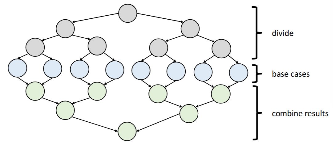
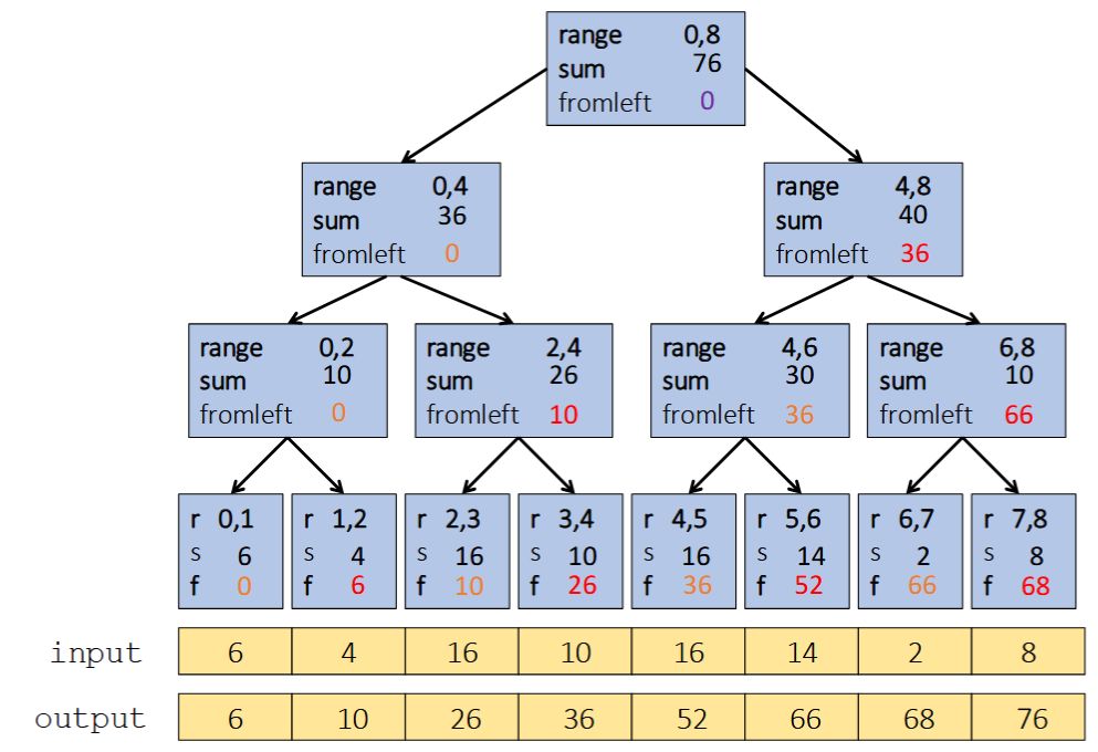
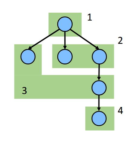
Second pass traverses the tree top-down: the "down" pass
Each pass has \(O(n)\) work and \(O(\log n)\) span So in total there is \(O(n)\) work and \(O(\log n)\) span So like with array summing, parallelism is \(n / \log n\)
Field-by-field Comparison
Field
Before
After
Text
<b>Parallel prefix-sum</b>
<br><br>
The parallel-prefix algorithm does two passes:<br><ol><li>
First pass {{c1::builds a tree bottom-up: the "up" pass}}</li><li>
Second pass {{c1::traverses the tree top-down: the "down" pass}}</li></ol>
Extra
Each pass has \(O(n)\) work and \(O(\log n)\) span<br>So in total there is \(O(n)\) work and \(O(\log n)\) span<br>So like with array summing, parallelism is \(n / \log n\)<br><br><div><img src="paste-c29833901d0bef4bf829b08f15583acc2ac94c68.jpg"><br></div>
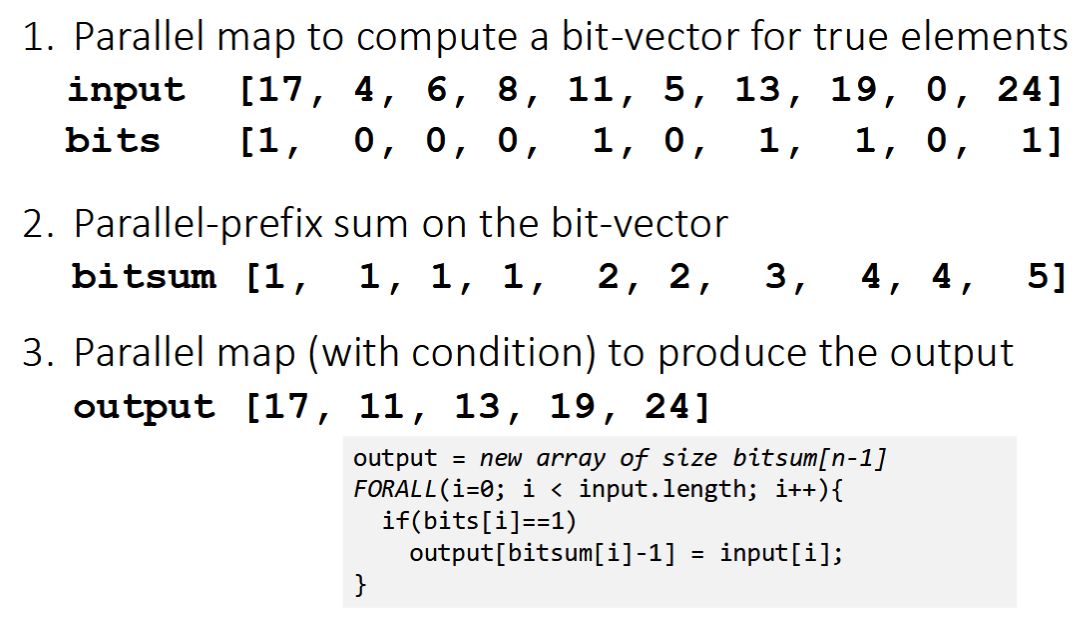
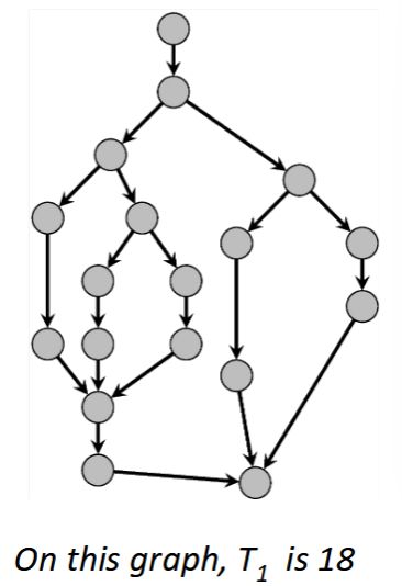
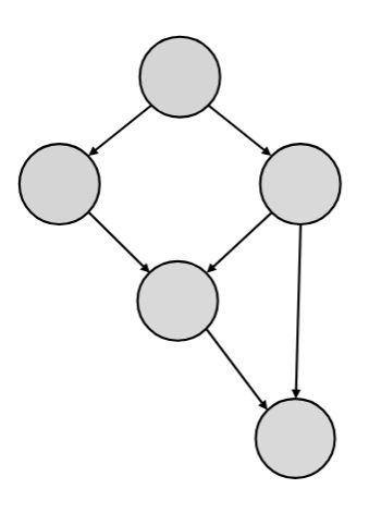
Gives an upper bound on how much speedup we can get
On this graph: \(T_1 / T_\infty = 18 / 9 = 2\)
This means that even with infinite cores and threads, the best possible speedup is 2.
Bottleneck is the span – DAG structure does not allow more parallelism.
Field-by-field Comparison
Field
Before
After
Text
Parallelism in DAG = \({{c1::T_1 / T_\infty}}\)
<ul>
<li>How much parallelism exist in the task graph</li>
<li>Gives an upper bound on how much speedup we can get</li>
</ul>
Extra
<img src="paste-ec818a1d799c2a19ea6cad709291b848ccaa132c.jpg" style="float: right;">On this graph: \(T_1 / T_\infty = 18 / 9 = 2\)
<br><br>
This means that even with infinite cores and threads, the best possible speedup is 2.<br><br>
Bottleneck is the span – DAG structure does not allow more parallelism.
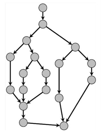
A program execution using fork and join can be seen as a DAG.
Nodes: Units of work
FJ: tasks; Cilk: finer-grained strands
Edges: Dependencies
Source must finish before destination starts (logical completion, not immediate termination)
The DAG does not depict "who is running when", but rather "who must finish before what"
Field-by-field Comparison
Field
Before
After
Text
A program execution using fork and join can be seen as a {{c1::DAG}}.
Extra
<img src="paste-5f03284709dc83297ef59e92187f035b0919be20.jpg" style="float: right;">Nodes: Units of work<br><ul><li>FJ: tasks; Cilk: finer-grained strands</li></ul>Edges: Dependencies<br><ul><li>Source must finish before destination starts (logical completion, not immediate termination)</li></ul><div>The DAG does not depict "who is running when", but rather "who must finish before what"<br></div>
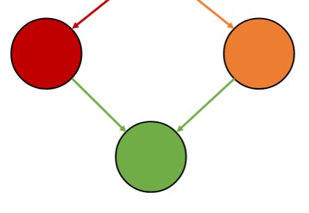
A join after a fork creates a node with two incoming edges:
One from the forked task that just finished
One from the continuation of the original task (which was waiting for the forked task to complete)
The continuation does not execute until both branches leading into the join node are complete.
Field-by-field Comparison
Field
Before
After
Text
A join after a fork creates a node with two incoming edges:<br><ul><li>One from {{c1::the forked task that just finished}}</li><li>One from {{c2::the continuation of the original task (which was waiting for the forked task to complete)}}</li></ul>
Extra
<img src="paste-1ce0eec3f1632895953635ebfd77d792ac16328e.jpg"><br><br>The continuation does not execute until both branches leading into the join node are complete.
A wide task graph → higher potential parallelism (shorter \(T_\infty\))
A deep task graph → more sequential dependencies (longer \(T_\infty\), less speedup)
Speedup is limited by the ratio \(T_1 / T_\infty\) (work versus critical path → Amdahl's law).
Parallelism is limited by dependencies.
Field-by-field Comparison
Field
Before
After
Text
Intuition from the DAG:<br><ul><li>A wide task graph → {{c1::higher potential parallelism (shorter \(T_\infty\))}}</li><li>
A deep task graph → {{c1::more sequential dependencies (longer \(T_\infty\), less speedup)}}</li></ul>
Extra
Speedup is limited by the ratio \(T_1 / T_\infty\) (work versus critical path → Amdahl's law).<br><br>
Parallelism is limited by dependencies.
Designing parallel algorithms is about decreasing span without increasing work too much.
Amdahl's Law describes the limit of speedup due to sequential parts of a program
\(T_\infty\) (span) in the DAG is the practical representation of the "sequential fraction" in Amdahl's Law
\(T_\infty\) is the fundamental cause of the speedup limit - it represents the longest sequential dependency
If we reduce \(T_\infty\), we get closer to ideal speedup
Field-by-field Comparison
Field
Before
After
Text
Designing parallel algorithms is about {{c1::decreasing span without increasing work too much}}.
Extra
<ol><li>Amdahl's Law describes the limit of speedup due to sequential parts of a program</li>
<li>\(T_\infty\) (span) in the DAG is the practical representation of the "sequential fraction" in Amdahl's Law</li>
<li>\(T_\infty\) is the fundamental cause of the speedup limit - it represents the longest sequential dependency</li>
<li>If we reduce \(T_\infty\), we get closer to ideal speedup</li></ol>
We can control p by configuring the thread pool (ForkJoinPool(p))
We cannot control \(T_p\) - it depends on:
Task dependencies in the DAG
Work distribution and load balancing
Thread contention and scheduling by the JVM/OS
Field-by-field Comparison
Field
Before
After
Text
\(T_p\) in DAG: execution time on p threads
<ul>
<li>We can control p by {{c1::configuring the thread pool (<code>ForkJoinPool(p)</code>)}}</li>
<li>We cannot control \(T_p\) - it depends on:
<ul>
<li>{{c2::Task dependencies in the DAG}}</li>
<li>{{c2::Work distribution and load balancing}}</li>
<li>{{c2::Thread contention and scheduling by the JVM/OS}}</li>
</ul>
</li>
</ul>
For parallelism, balanced trees are generally better than lists so that we can get to all the data exponentially faster (\(O(\log n)\) vs. \(O(n)\)).
Trees have the same flexibility as lists compared to arrays.
Field-by-field Comparison
Field
Before
After
Text
For parallelism, balanced trees are generally {{c1::better::better/worse}} than lists so that {{c1::we can get to all the data exponentially faster (\(O(\log n)\) vs. \(O(n)\))}}.
Extra
Trees have the same flexibility as lists compared to arrays.
First two steps can be combined into one pass
<ul>
<li>Just using a different base case for the prefix sum</li>
<li>No effect on asymptotic complexity</li>
</ul>
Can also combine third step into the down pass of the prefix sum
<ul>
<li>Again no effect on asymptotic complexity</li>
</ul>
Analysis: \(O(n)\) work, \(O(\log n)\) span
<ul>
<li>2 or 3 passes, but 3 is a constant</li>
</ul>
We know a pack is \(O(n)\) work, \(O(\log n)\) span
Pack elements less than pivot into left side of aux array
Pack elements greater than pivot into right side of aux array
Put pivot between them and recursively sort
With a little more cleverness, can do both packs at once but no effect on asymptotic complexity
With \(O(\log n)\) span for partition, the total span for quicksort is \(T(n) = O(\log n) + 1T(n/2) = O(\log^2 n)\).
Parallelism is \(O(n \log n) / O(\log^2 n) = O(n / \log n)\).
Field-by-field Comparison
Field
Before
After
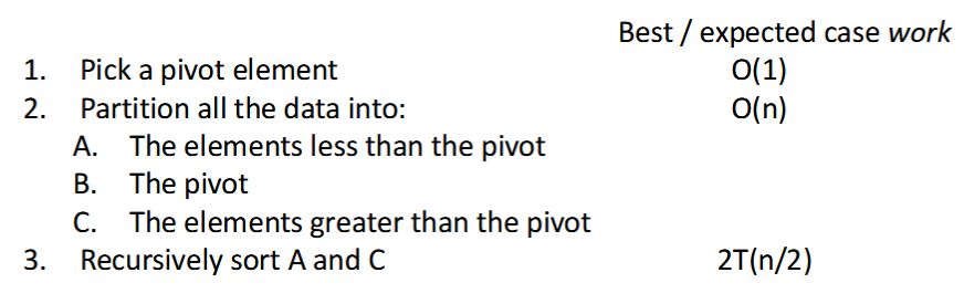
Front
For Quicksort, we partition all the data into:
<ol type="A">
<li>The elements less than the pivot</li>
<li>The pivot</li>
<li>The elements greater than the pivot</li>
</ol><div>How can this be parallelized?</div>
Back
This is just two packs!
<ul>
<li>We know a pack is \(O(n)\) work, \(O(\log n)\) span</li>
<li>Pack elements less than pivot into left side of <code>aux</code> array</li>
<li>Pack elements greater than pivot into right side of <code>aux</code> array</li>
<li>Put pivot between them and recursively sort</li>
<li>With a little more cleverness, can do both packs at once but no effect on asymptotic complexity</li>
</ul>
With \(O(\log n)\) span for partition, the total span for quicksort is \(T(n) = O(\log n) + 1T(n/2) = O(\log^2 n)\).<br>
Parallelism is \(O(n \log n) / O(\log^2 n) = O(n / \log n)\).
A fork ends a node and creates two outgoing edges:
One to a new forked task
One to the continuation of the current task
May execute in parallel if worker thread is available.
Field-by-field Comparison
Field
Before
After
Text
A fork ends a node and creates two outgoing edges:<br><ul><li>One to {{c1::a new forked task}}</li><li>One to {{c1::the continuation of the current task}}</li></ul>
Extra
<img src="paste-cea411eff84adb49b099f7aa3bad8e51a3f80d02.jpg"><br><br>May execute in parallel if worker thread is available.
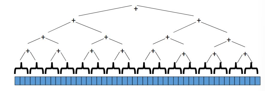
So parallelism (i.e., work / span) is \(O(\log n)\)
Field-by-field Comparison
Field
Before
After
Front
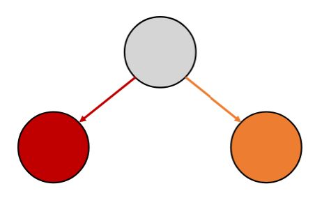
How can we parallelize Quicksort?<br><br><img src="paste-2e1c682cea6540c1e39b1511df2d33cbcc697698.jpg">
Back
Easy: Do the two recursive calls in parallel
<ul>
<li>Work: unchanged of course \(O(n \log n)\)</li>
<li>Span: now \(T(n) = O(n) + 1T(n/2) = O(n)\)</li>
<li>So parallelism (i.e., work / span) is \(O(\log n)\)</li>
</ul>
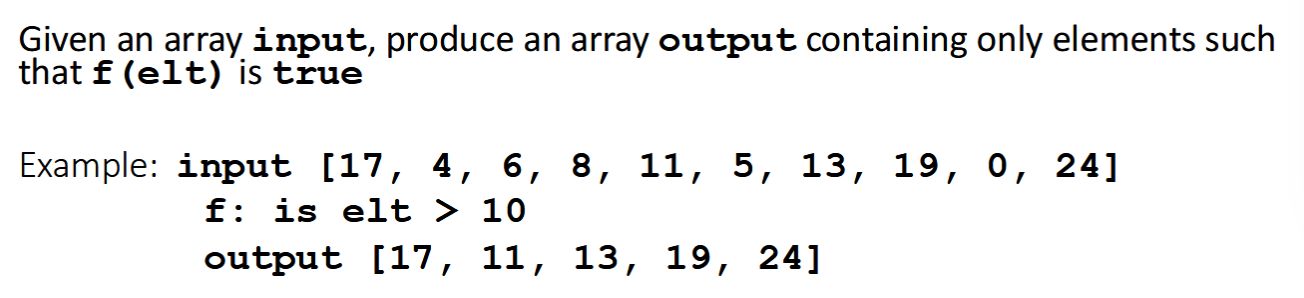
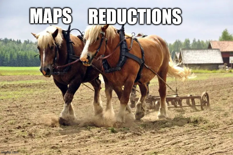
Reductions produce a single answer from a collection via an associative operator.
Examples: max, count, rightmost, sum.
Field-by-field Comparison
Field
Before
After
Text
{{c1::Reductions}} produce a {{c2::single answer}} from a collection via an {{c3::associative operator}}. Examples: {{c4::max, count, rightmost, sum}}.
{{c1::Reductions}} produce {{c2::a single answer from a collection via an associative operator}}.
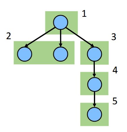
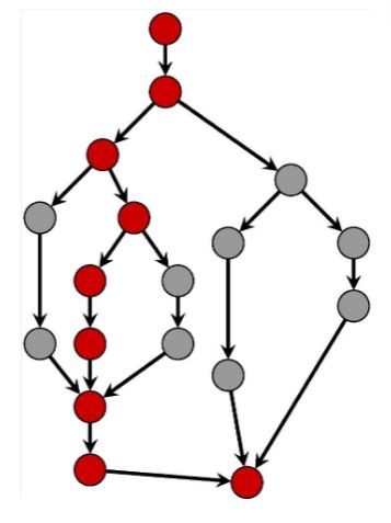
Spawn other tasks (= start in JT, submit in ExS, fork in FJ)
Wait for results from other tasks (= join in JT and FJ, get in ExS)
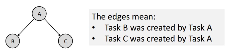
A graph is formed based on spawning tasks:
Field-by-field Comparison
Field
Before
After
Text
Tasks:<br><ol><li>Execute code</li><li>{{c1::Spawn other tasks (= start in JT, submit in ExS, fork in FJ)}}</li><li>{{c2::Wait for results from other tasks (= join in JT and FJ, get in ExS)}}</li></ol>
Extra
A graph is formed based on spawning tasks:<br><br><img src="paste-49c881948e5bf3f307be6ad2f1a2946538f4da1a.jpg">
 On this graph: \(T_1 / T_\infty = 18 / 9 = 2\)
 Nodes: Units of work