Note 1: ETH::2. Semester::A&W
Deck: ETH::2. Semester::A&W
Note Type: Horvath Cloze
GUID: A-7$#*Ia_p
modified
Before
Front
ETH::2._Semester::A&W::2._Wahrscheinlichkeitstheorie_und_randomisierte_Algorithmen::2._Bedingte_Wahrscheinlichkeiten
Seien \(A\) und \(B\) Ereignisse mit \(\Pr[B] > 0\).
Die bedingte Wahrscheinlichkeit \(\Pr[A|B]\) von \(A\) gegeben \(B\) ist definiert durch
\[\Pr[A|B] := {{c1::\frac{\Pr[A \cap B]}{\Pr[B]} }}\]
Back
ETH::2._Semester::A&W::2._Wahrscheinlichkeitstheorie_und_randomisierte_Algorithmen::2._Bedingte_Wahrscheinlichkeiten
Seien \(A\) und \(B\) Ereignisse mit \(\Pr[B] > 0\).
Die bedingte Wahrscheinlichkeit \(\Pr[A|B]\) von \(A\) gegeben \(B\) ist definiert durch
\[\Pr[A|B] := {{c1::\frac{\Pr[A \cap B]}{\Pr[B]} }}\]
After
Front
ETH::2._Semester::A&W::2._Wahrscheinlichkeitstheorie_und_randomisierte_Algorithmen::2._Bedingte_Wahrscheinlichkeiten
Seien \(A\) und \(B\) Ereignisse mit \(\Pr[B] > 0\).
Die bedingte Wahrscheinlichkeit \(\Pr[A|B]\) von \(A\) gegeben \(B\) ist definiert durch: \[\Pr[A|B] := {{c1::\frac{\Pr[A \cap B]}{\Pr[B]} }}\]
Back
ETH::2._Semester::A&W::2._Wahrscheinlichkeitstheorie_und_randomisierte_Algorithmen::2._Bedingte_Wahrscheinlichkeiten
Seien \(A\) und \(B\) Ereignisse mit \(\Pr[B] > 0\).
Die bedingte Wahrscheinlichkeit \(\Pr[A|B]\) von \(A\) gegeben \(B\) ist definiert durch: \[\Pr[A|B] := {{c1::\frac{\Pr[A \cap B]}{\Pr[B]} }}\]
Field-by-field Comparison
| Field |
Before |
After |
| Text |
Seien \(A\) und \(B\) Ereignisse mit \(\Pr[B] > 0\).
<br><br>
Die bedingte Wahrscheinlichkeit \(\Pr[A|B]\) von \(A\) gegeben \(B\) ist definiert durch
\[\Pr[A|B] := {{c1::\frac{\Pr[A \cap B]}{\Pr[B]} }}\] |
Seien \(A\) und \(B\) Ereignisse mit \(\Pr[B] > 0\).
<br><br>
Die bedingte Wahrscheinlichkeit \(\Pr[A|B]\) von \(A\) gegeben \(B\) ist definiert durch: \[\Pr[A|B] := {{c1::\frac{\Pr[A \cap B]}{\Pr[B]} }}\] |
Tags:
ETH::2._Semester::A&W::2._Wahrscheinlichkeitstheorie_und_randomisierte_Algorithmen::2._Bedingte_Wahrscheinlichkeiten
Note 2: ETH::2. Semester::A&W
Deck: ETH::2. Semester::A&W
Note Type: Horvath Cloze
GUID: B1cEOSgE
modified
Before
Front
ETH::2._Semester::A&W::1._Graphentheorie::6._Matchings::1._Algorithmen
BFS für augmentierende Pfade in bipartiten Graphen \(G = (A \uplus B, E)\):
- \(L_0 := \)unüberdeckte Knoten aus \(A\)
- Für ungerades \(i\): \(L_i := \){{c2::unbesuchte Nachbarn von \(L_{i-1}\) via Kanten in \(E \setminus M\)}}
- Für gerades \(i\): \(L_i := \){{c3::unbesuchte Nachbarn von \(L_{i-1}\) via Kanten in \(M\)}}
- Terminierung: sobald \(L_i\) einen unüberdeckten Knoten enthält → Pfad per Backtracking.
Back
ETH::2._Semester::A&W::1._Graphentheorie::6._Matchings::1._Algorithmen
BFS für augmentierende Pfade in bipartiten Graphen \(G = (A \uplus B, E)\):
- \(L_0 := \)unüberdeckte Knoten aus \(A\)
- Für ungerades \(i\): \(L_i := \){{c2::unbesuchte Nachbarn von \(L_{i-1}\) via Kanten in \(E \setminus M\)}}
- Für gerades \(i\): \(L_i := \){{c3::unbesuchte Nachbarn von \(L_{i-1}\) via Kanten in \(M\)}}
- Terminierung: sobald \(L_i\) einen unüberdeckten Knoten enthält → Pfad per Backtracking.
Laufzeit: \(O(|V| + |E|)\) für einen augmentierenden Pfad.
After
Front
ETH::2._Semester::A&W::1._Graphentheorie::6._Matchings::1._Algorithmen
BFS für augmentierende Pfade in bipartiten Graphen \(G = (A \uplus B, E)\):
- \(L_0 := \) unüberdeckte Knoten aus \(A\)
- Für ungerades \(i\): \(L_i := \) {{c2::unbesuchte Nachbarn von \(L_{i-1}\) via Kanten in \(E \setminus M\)}}
- Für gerades \(i\): \(L_i := \) {{c2::unbesuchte Nachbarn von \(L_{i-1}\) via Kanten in \(M\)}}
- Terminierung: Sobald \(L_i\) einen unüberdeckten Knoten enthält → Pfad per Backtracking.
Back
ETH::2._Semester::A&W::1._Graphentheorie::6._Matchings::1._Algorithmen
BFS für augmentierende Pfade in bipartiten Graphen \(G = (A \uplus B, E)\):
- \(L_0 := \) unüberdeckte Knoten aus \(A\)
- Für ungerades \(i\): \(L_i := \) {{c2::unbesuchte Nachbarn von \(L_{i-1}\) via Kanten in \(E \setminus M\)}}
- Für gerades \(i\): \(L_i := \) {{c2::unbesuchte Nachbarn von \(L_{i-1}\) via Kanten in \(M\)}}
- Terminierung: Sobald \(L_i\) einen unüberdeckten Knoten enthält → Pfad per Backtracking.
Laufzeit: \(O(|V| + |E|)\) für einen augmentierenden Pfad.
Field-by-field Comparison
| Field |
Before |
After |
| Text |
BFS für augmentierende Pfade in bipartiten Graphen \(G = (A \uplus B, E)\):<br><ol><li>\(L_0 := \){{c1::unüberdeckte Knoten aus \(A\)}}</li><li>Für ungerades \(i\): \(L_i := \){{c2::unbesuchte Nachbarn von \(L_{i-1}\) via Kanten in \(E \setminus M\)}}</li><li>Für gerades \(i\): \(L_i := \){{c3::unbesuchte Nachbarn von \(L_{i-1}\) via Kanten in \(M\)}}</li><li>Terminierung: {{c4::sobald \(L_i\) einen unüberdeckten Knoten enthält}} → Pfad per Backtracking.</li></ol> |
BFS für augmentierende Pfade in bipartiten Graphen \(G = (A \uplus B, E)\):<br><ol><li>\(L_0 := \) {{c1::unüberdeckte Knoten aus \(A\)}}</li><li>Für ungerades \(i\): \(L_i := \) {{c2::unbesuchte Nachbarn von \(L_{i-1}\) via Kanten in \(E \setminus M\)}}</li><li>Für gerades \(i\): \(L_i := \) {{c2::unbesuchte Nachbarn von \(L_{i-1}\) via Kanten in \(M\)}}</li><li>Terminierung: {{c4::Sobald \(L_i\) einen unüberdeckten Knoten enthält}} → Pfad per Backtracking.</li></ol> |
Tags:
ETH::2._Semester::A&W::1._Graphentheorie::6._Matchings::1._Algorithmen
Note 3: ETH::2. Semester::A&W
Deck: ETH::2. Semester::A&W
Note Type: Horvath Cloze
GUID: GDDu8@FRW=
modified
Before
Front
ETH::2._Semester::A&W::2._Wahrscheinlichkeitstheorie_und_randomisierte_Algorithmen::4._Zufallsvariablen::3._Varianz
Die Grösse {{c1::\(\sigma := \sqrt{\operatorname{Var}[X]}\)}} heisst Standardabweichung von \(X\).
Back
ETH::2._Semester::A&W::2._Wahrscheinlichkeitstheorie_und_randomisierte_Algorithmen::4._Zufallsvariablen::3._Varianz
Die Grösse {{c1::\(\sigma := \sqrt{\operatorname{Var}[X]}\)}} heisst Standardabweichung von \(X\).
After
Front
ETH::2._Semester::A&W::2._Wahrscheinlichkeitstheorie_und_randomisierte_Algorithmen::4._Zufallsvariablen::3._Varianz
Die Grösse \(\sigma := {{c1::\sqrt{\operatorname{Var}[X]} }}\) heisst Standardabweichung von \(X\).
Back
ETH::2._Semester::A&W::2._Wahrscheinlichkeitstheorie_und_randomisierte_Algorithmen::4._Zufallsvariablen::3._Varianz
Die Grösse \(\sigma := {{c1::\sqrt{\operatorname{Var}[X]} }}\) heisst Standardabweichung von \(X\).
Field-by-field Comparison
| Field |
Before |
After |
| Text |
Die Grösse {{c1::\(\sigma := \sqrt{\operatorname{Var}[X]}\)}} heisst {{c2::Standardabweichung von \(X\)}}. |
Die Grösse \(\sigma := {{c1::\sqrt{\operatorname{Var}[X]} }}\) heisst {{c2::Standardabweichung von \(X\)}}. |
Tags:
ETH::2._Semester::A&W::2._Wahrscheinlichkeitstheorie_und_randomisierte_Algorithmen::4._Zufallsvariablen::3._Varianz
Note 4: ETH::2. Semester::A&W
Deck: ETH::2. Semester::A&W
Note Type: Horvath Cloze
GUID: GTMcPtrK9g
modified
Before
Front
basic ETH::2._Semester::A&W::2._Wahrscheinlichkeitstheorie_und_randomisierte_Algorithmen::0._Kombinatorik
Die Anzahl der geordneten Auswahlen von \(k\) aus \(n\) Objekten
mit Zurücklegen (Reihenfolge wichtig) ist:
\[n^k.\]
Back
basic ETH::2._Semester::A&W::2._Wahrscheinlichkeitstheorie_und_randomisierte_Algorithmen::0._Kombinatorik
Die Anzahl der geordneten Auswahlen von \(k\) aus \(n\) Objekten
mit Zurücklegen (Reihenfolge wichtig) ist:
\[n^k.\]
Jede der \(k\) Positionen hat \(n\) Möglichkeiten.
Beispiel:
Wie viele 4-stellige PINs aus 0–9 (mit Wiederholung)?
\(10^4 = 10{,}000\).
After
Front
basic ETH::2._Semester::A&W::2._Wahrscheinlichkeitstheorie_und_randomisierte_Algorithmen::0._Kombinatorik
Die Anzahl der geordneten Auswahlen von \(k\) aus \(n\) Objekten
mit Zurücklegen (Reihenfolge wichtig) ist:
\[n^k\]
Back
basic ETH::2._Semester::A&W::2._Wahrscheinlichkeitstheorie_und_randomisierte_Algorithmen::0._Kombinatorik
Die Anzahl der geordneten Auswahlen von \(k\) aus \(n\) Objekten
mit Zurücklegen (Reihenfolge wichtig) ist:
\[n^k\]
Jede der \(k\) Positionen hat \(n\) Möglichkeiten.
Beispiel:
Wie viele 4-stellige PINs aus 0–9 (mit Wiederholung)?
\(10^4 = 10{,}000\).
Field-by-field Comparison
| Field |
Before |
After |
| Text |
Die Anzahl der geordneten Auswahlen von \(k\) aus \(n\) Objekten<br><strong>mit Zurücklegen</strong> (Reihenfolge wichtig) ist:<br>\[{{c1::n^k}}.\] |
Die Anzahl der geordneten Auswahlen von \(k\) aus \(n\) Objekten<br><strong>mit Zurücklegen</strong> (Reihenfolge wichtig) ist:<br>\[{{c1::n^k}}\] |
Tags:
ETH::2._Semester::A&W::2._Wahrscheinlichkeitstheorie_und_randomisierte_Algorithmen::0._Kombinatorik
basic
Note 5: ETH::2. Semester::A&W
Deck: ETH::2. Semester::A&W
Note Type: Horvath Cloze
GUID: H#LoquJg]}
modified
Before
Front
basic ETH::2._Semester::A&W::2._Wahrscheinlichkeitstheorie_und_randomisierte_Algorithmen::0._Kombinatorik
Für den Binomialkoeffizienten gilt:
\(\binom{n}{k} = {{c1::\binom{n}{n-k} :: symmetrie }}\)
Back
basic ETH::2._Semester::A&W::2._Wahrscheinlichkeitstheorie_und_randomisierte_Algorithmen::0._Kombinatorik
Für den Binomialkoeffizienten gilt:
\(\binom{n}{k} = {{c1::\binom{n}{n-k} :: symmetrie }}\)
After
Front
basic ETH::2._Semester::A&W::2._Wahrscheinlichkeitstheorie_und_randomisierte_Algorithmen::0._Kombinatorik
Für den Binomialkoeffizienten gilt:\[\binom{n}{k} = {{c1::\binom{n}{n-k} :: \text{Symmetrie} }}\]
Back
basic ETH::2._Semester::A&W::2._Wahrscheinlichkeitstheorie_und_randomisierte_Algorithmen::0._Kombinatorik
Für den Binomialkoeffizienten gilt:\[\binom{n}{k} = {{c1::\binom{n}{n-k} :: \text{Symmetrie} }}\]
Field-by-field Comparison
| Field |
Before |
After |
| Text |
Für den Binomialkoeffizienten gilt:<br>\(\binom{n}{k} = {{c1::\binom{n}{n-k} :: symmetrie }}\) |
Für den Binomialkoeffizienten gilt:\[\binom{n}{k} = {{c1::\binom{n}{n-k} :: \text{Symmetrie} }}\] |
Tags:
ETH::2._Semester::A&W::2._Wahrscheinlichkeitstheorie_und_randomisierte_Algorithmen::0._Kombinatorik
basic
Note 6: ETH::2. Semester::A&W
Deck: ETH::2. Semester::A&W
Note Type: Horvath Cloze
GUID: HmM2`t+Bg|
modified
Before
Front
ETH::2._Semester::A&W::2._Wahrscheinlichkeitstheorie_und_randomisierte_Algorithmen::4._Zufallsvariablen::3._Varianz
Für Die Varianz gilt \[\mathbb{E}[(X - \mu)^2] = {{c1::\sum_{x \in W_X} (x - \mu)^2 \cdot \Pr[X = x]::summenform}}\]
Back
ETH::2._Semester::A&W::2._Wahrscheinlichkeitstheorie_und_randomisierte_Algorithmen::4._Zufallsvariablen::3._Varianz
Für Die Varianz gilt \[\mathbb{E}[(X - \mu)^2] = {{c1::\sum_{x \in W_X} (x - \mu)^2 \cdot \Pr[X = x]::summenform}}\]
After
Front
ETH::2._Semester::A&W::2._Wahrscheinlichkeitstheorie_und_randomisierte_Algorithmen::4._Zufallsvariablen::3._Varianz
Für die Varianz gilt: \[\mathbb{E}[(X - \mu)^2] = {{c1::\sum_{x \in W_X} (x - \mu)^2 \cdot \Pr[X = x]::\text{Summe} }}\]
Back
ETH::2._Semester::A&W::2._Wahrscheinlichkeitstheorie_und_randomisierte_Algorithmen::4._Zufallsvariablen::3._Varianz
Für die Varianz gilt: \[\mathbb{E}[(X - \mu)^2] = {{c1::\sum_{x \in W_X} (x - \mu)^2 \cdot \Pr[X = x]::\text{Summe} }}\]
Field-by-field Comparison
| Field |
Before |
After |
| Text |
Für Die Varianz gilt \[\mathbb{E}[(X - \mu)^2] = {{c1::\sum_{x \in W_X} (x - \mu)^2 \cdot \Pr[X = x]::summenform}}\]<br> |
Für die Varianz gilt: \[\mathbb{E}[(X - \mu)^2] = {{c1::\sum_{x \in W_X} (x - \mu)^2 \cdot \Pr[X = x]::\text{Summe} }}\] |
Tags:
ETH::2._Semester::A&W::2._Wahrscheinlichkeitstheorie_und_randomisierte_Algorithmen::4._Zufallsvariablen::3._Varianz
Note 7: ETH::2. Semester::A&W
Deck: ETH::2. Semester::A&W
Note Type: Horvath Cloze
GUID: Kxi,Zs1MD]
modified
Before
Front
ETH::2._Semester::A&W::1._Graphentheorie::7._Färbungen
\(G \neq
K_n,\ G \neq {{c1::C_{2n+1} }},\ G\) zshgd.:
\(\Rightarrow\) \(G\) kann in Zeit \(O(|E|)\) mit \(\Delta(G)\) Farben gefärbt werden
Back
ETH::2._Semester::A&W::1._Graphentheorie::7._Färbungen
\(G \neq
K_n,\ G \neq {{c1::C_{2n+1} }},\ G\) zshgd.:
\(\Rightarrow\) \(G\) kann in Zeit \(O(|E|)\) mit \(\Delta(G)\) Farben gefärbt werden
Satz von Brooks
\(K_n\) ist der vollständige Graph auf (n) Knoten - jeder Knoten ist mit jedem anderen verbunden. Er braucht \(n\) Farben.
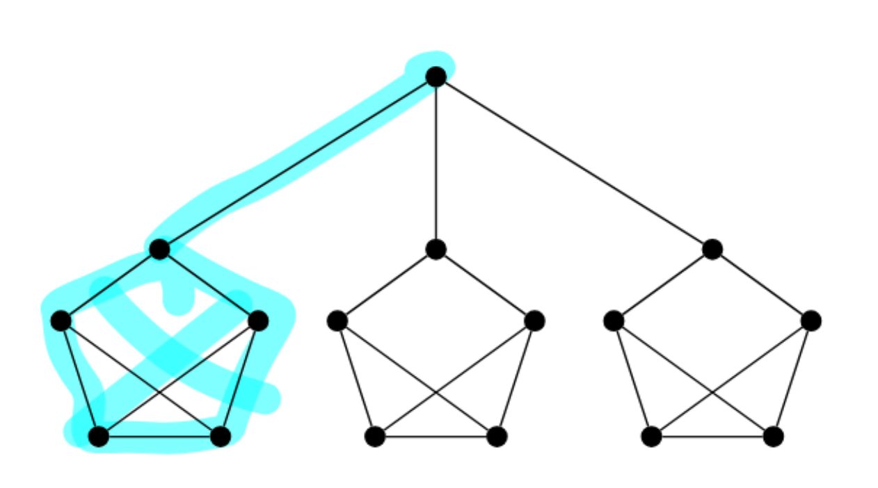
\(C_{2n+1}\) ist ein Kreis mit einer ungeraden Anzahl von Knoten (z.B. Dreieck, Fünfeck, ...). Er braucht 3 Farben, obwohl \(\Delta = 2\).
After
Front
ETH::2._Semester::A&W::1._Graphentheorie::7._Färbungen
\(G \neq
K_n,\ G \neq {{c1::C_{2n+1} }},\ G\) zshgd.:
\(\Rightarrow\) \(G\) kann in Zeit \(O(|E|)\) mit \(\Delta(G)\) Farben gefärbt werden
Back
ETH::2._Semester::A&W::1._Graphentheorie::7._Färbungen
\(G \neq
K_n,\ G \neq {{c1::C_{2n+1} }},\ G\) zshgd.:
\(\Rightarrow\) \(G\) kann in Zeit \(O(|E|)\) mit \(\Delta(G)\) Farben gefärbt werden
Satz von Brooks
\(K_n\) ist der vollständige Graph auf \(n\) Knoten - jeder Knoten ist mit jedem anderen verbunden. Er braucht \(n\) Farben.
\(C_{2n+1}\) ist ein Kreis mit einer ungeraden Anzahl von Knoten (z.B. Dreieck, Fünfeck, ...). Er braucht 3 Farben, obwohl \(\Delta = 2\).
Field-by-field Comparison
| Field |
Before |
After |
| Extra |
Satz von Brooks<br><br><div>\(K_n\) ist der vollständige Graph auf (n) Knoten - jeder Knoten ist mit jedem anderen verbunden. Er braucht \(n\) Farben.</div>
<div>\(C_{2n+1}\) ist ein Kreis mit einer ungeraden Anzahl von Knoten (z.B. Dreieck, Fünfeck, ...). Er braucht 3 Farben, obwohl \(\Delta = 2\).</div> |
Satz von Brooks<br><br><div>\(K_n\) ist der vollständige Graph auf \(n\) Knoten - jeder Knoten ist mit jedem anderen verbunden. Er braucht \(n\) Farben.</div>
<div>\(C_{2n+1}\) ist ein Kreis mit einer ungeraden Anzahl von Knoten (z.B. Dreieck, Fünfeck, ...). Er braucht 3 Farben, obwohl \(\Delta = 2\).</div> |
Tags:
ETH::2._Semester::A&W::1._Graphentheorie::7._Färbungen
Note 8: ETH::2. Semester::A&W
Deck: ETH::2. Semester::A&W
Note Type: Horvath Cloze
GUID: LE!#OdHaHH
modified
Before
Front
ETH::2._Semester::A&W::2._Wahrscheinlichkeitstheorie_und_randomisierte_Algorithmen::4._Zufallsvariablen::2._Erwartungswert
Die Linearität der Erwartung hält wenn \(X_1,\ldots,X_n\) nicht unabhängig, du dummbatzi sind?
Back
ETH::2._Semester::A&W::2._Wahrscheinlichkeitstheorie_und_randomisierte_Algorithmen::4._Zufallsvariablen::2._Erwartungswert
Die Linearität der Erwartung hält wenn \(X_1,\ldots,X_n\) nicht unabhängig, du dummbatzi sind?
After
Front
ETH::2._Semester::A&W::2._Wahrscheinlichkeitstheorie_und_randomisierte_Algorithmen::4._Zufallsvariablen::2._Erwartungswert
Die Linearität der Erwartung hält, wenn \(X_1,\ldots,X_n\) vollkommen wurscht ob unabhängig, du dummbatzi sind?
Back
ETH::2._Semester::A&W::2._Wahrscheinlichkeitstheorie_und_randomisierte_Algorithmen::4._Zufallsvariablen::2._Erwartungswert
Die Linearität der Erwartung hält, wenn \(X_1,\ldots,X_n\) vollkommen wurscht ob unabhängig, du dummbatzi sind?
Field-by-field Comparison
| Field |
Before |
After |
| Text |
Die Linearität der Erwartung hält wenn \(X_1,\ldots,X_n\) {{c1::nicht unabhängig, du dummbatzi}} sind? |
Die Linearität der Erwartung hält, wenn \(X_1,\ldots,X_n\) {{c1::vollkommen wurscht ob unabhängig, du dummbatzi}} sind? |
Tags:
ETH::2._Semester::A&W::2._Wahrscheinlichkeitstheorie_und_randomisierte_Algorithmen::4._Zufallsvariablen::2._Erwartungswert
Note 9: ETH::2. Semester::A&W
Deck: ETH::2. Semester::A&W
Note Type: Horvath Cloze
GUID: P#e48Dok$?
modified
Before
Front
ETH::2._Semester::A&W::2._Wahrscheinlichkeitstheorie_und_randomisierte_Algorithmen::3._Unabhängigkeit
Paarweise Unabhängigkeit \(\not\Rightarrow\) aber \(\Leftarrow\) stochastische Unabhängigkeit!
Back
ETH::2._Semester::A&W::2._Wahrscheinlichkeitstheorie_und_randomisierte_Algorithmen::3._Unabhängigkeit
Paarweise Unabhängigkeit \(\not\Rightarrow\) aber \(\Leftarrow\) stochastische Unabhängigkeit!
After
Front
ETH::2._Semester::A&W::2._Wahrscheinlichkeitstheorie_und_randomisierte_Algorithmen::3._Unabhängigkeit
Paarweise Unabhängigkeit \(\Leftarrow\) Stochastische Unabhängigkeit
Back
ETH::2._Semester::A&W::2._Wahrscheinlichkeitstheorie_und_randomisierte_Algorithmen::3._Unabhängigkeit
Paarweise Unabhängigkeit \(\Leftarrow\) Stochastische Unabhängigkeit
Field-by-field Comparison
| Field |
Before |
After |
| Text |
Paarweise Unabhängigkeit {{c1::\(\not\Rightarrow\) aber \(\Leftarrow\)}} stochastische Unabhängigkeit! |
Paarweise Unabhängigkeit {{c1::\(\Leftarrow\)::Implikationen in welche Richtungen?}} Stochastische Unabhängigkeit |
Tags:
ETH::2._Semester::A&W::2._Wahrscheinlichkeitstheorie_und_randomisierte_Algorithmen::3._Unabhängigkeit
Note 10: ETH::2. Semester::A&W
Deck: ETH::2. Semester::A&W
Note Type: Horvath Cloze
GUID: P<77mx`t+b
modified
Before
Front
ETH::2._Semester::A&W::2._Wahrscheinlichkeitstheorie_und_randomisierte_Algorithmen::4._Zufallsvariablen::3._Varianz
Für eine Zufallsvariable \(X\) mit \(\mu = \mathbb{E}[X]\) definieren wir die Varianz \(\operatorname{Var}[X]\) durch \[\operatorname{Var}[X] := {{c1::\mathbb{E}[(X - \mu)^2]}}\]
Back
ETH::2._Semester::A&W::2._Wahrscheinlichkeitstheorie_und_randomisierte_Algorithmen::4._Zufallsvariablen::3._Varianz
Für eine Zufallsvariable \(X\) mit \(\mu = \mathbb{E}[X]\) definieren wir die Varianz \(\operatorname{Var}[X]\) durch \[\operatorname{Var}[X] := {{c1::\mathbb{E}[(X - \mu)^2]}}\]
After
Front
ETH::2._Semester::A&W::2._Wahrscheinlichkeitstheorie_und_randomisierte_Algorithmen::4._Zufallsvariablen::3._Varianz
Für eine Zufallsvariable \(X\) mit \(\mu = \mathbb{E}[X]\) definieren wir die Varianz \(\operatorname{Var}[X]\) durch: \[\operatorname{Var}[X] := {{c1::\mathbb{E}[(X - \mu)^2]}}\]
Back
ETH::2._Semester::A&W::2._Wahrscheinlichkeitstheorie_und_randomisierte_Algorithmen::4._Zufallsvariablen::3._Varianz
Für eine Zufallsvariable \(X\) mit \(\mu = \mathbb{E}[X]\) definieren wir die Varianz \(\operatorname{Var}[X]\) durch: \[\operatorname{Var}[X] := {{c1::\mathbb{E}[(X - \mu)^2]}}\]
Field-by-field Comparison
| Field |
Before |
After |
| Text |
Für eine Zufallsvariable \(X\) mit \(\mu = \mathbb{E}[X]\) definieren wir die Varianz \(\operatorname{Var}[X]\) durch \[\operatorname{Var}[X] := {{c1::\mathbb{E}[(X - \mu)^2]}}\] |
Für eine Zufallsvariable \(X\) mit \(\mu = \mathbb{E}[X]\) definieren wir die Varianz \(\operatorname{Var}[X]\) durch: \[\operatorname{Var}[X] := {{c1::\mathbb{E}[(X - \mu)^2]}}\] |
Tags:
ETH::2._Semester::A&W::2._Wahrscheinlichkeitstheorie_und_randomisierte_Algorithmen::4._Zufallsvariablen::3._Varianz
Note 11: ETH::2. Semester::A&W
Deck: ETH::2. Semester::A&W
Note Type: Horvath Cloze
GUID: PV7-/GzLwe
modified
Before
Front
ETH::2._Semester::A&W::2._Wahrscheinlichkeitstheorie_und_randomisierte_Algorithmen::0._Kombinatorik
Rekursion (Pascalsches Dreieck): \(\binom{n}{k} = {{c3::\binom{n-1}{k-1} + \binom{n-1}{k} }}\)
Back
ETH::2._Semester::A&W::2._Wahrscheinlichkeitstheorie_und_randomisierte_Algorithmen::0._Kombinatorik
Rekursion (Pascalsches Dreieck): \(\binom{n}{k} = {{c3::\binom{n-1}{k-1} + \binom{n-1}{k} }}\)
After
Front
ETH::2._Semester::A&W::2._Wahrscheinlichkeitstheorie_und_randomisierte_Algorithmen::0._Kombinatorik
Die Rekursionsformel des Pascalschen Dreiecks lautet: \[\binom{n}{k} = {{c3::\binom{n-1}{k-1} + \binom{n-1}{k} }}\]
Back
ETH::2._Semester::A&W::2._Wahrscheinlichkeitstheorie_und_randomisierte_Algorithmen::0._Kombinatorik
Die Rekursionsformel des Pascalschen Dreiecks lautet: \[\binom{n}{k} = {{c3::\binom{n-1}{k-1} + \binom{n-1}{k} }}\]
Intuition: Fixiere Element \(x\).
- \(x\) dabei → noch \(k-1\) aus \(n-1\) wählen
- \(x\) nicht dabei → alle \(k\) aus \(n-1\) wählen
Pascalsches Dreieck (Eintrag in Zeile \(n\)
, Position \(k\)
ist \(\binom{n}{k}\)
):\[\begin{array}{ccccccccc} & & & & 1 \\ & & & 1 & & 1 \\ & & 1 & & 2 & & 1 \\ & 1 & & 3 & & 3 & & 1 \\ 1 & & 4 & & 6 & & 4 & & 1 \end{array}\]Jeder Eintrag = Summe der zwei Einträge schräg darüber.
Z.B.: \(\binom{4}{2} = 6 = \underbrace{\binom{3}{1}}_{3} + \underbrace{\binom{3}{2}}_{3}\)
Field-by-field Comparison
| Field |
Before |
After |
| Text |
Rekursion (Pascalsches Dreieck): \(\binom{n}{k} = {{c3::\binom{n-1}{k-1} + \binom{n-1}{k} }}\) |
Die Rekursionsformel des Pascalschen Dreiecks lautet: \[\binom{n}{k} = {{c3::\binom{n-1}{k-1} + \binom{n-1}{k} }}\] |
| Extra |
|
<b>Intuition:</b> <br>Fixiere Element \(x\).<br><ul><li>\(x\) dabei → noch \(k-1\) aus \(n-1\) wählen</li><li>\(x\) nicht dabei → alle \(k\) aus \(n-1\) wählen</li></ul><b>Pascalsches Dreieck (Eintrag in Zeile </b>\(n\)<b>, Position </b>\(k\)<b> ist </b>\(\binom{n}{k}\)<b>):</b><br>\[\begin{array}{ccccccccc} & & & & 1 \\ & & & 1 & & 1 \\ & & 1 & & 2 & & 1 \\ & 1 & & 3 & & 3 & & 1 \\ 1 & & 4 & & 6 & & 4 & & 1 \end{array}\]Jeder Eintrag = Summe der zwei Einträge schräg darüber.<br>Z.B.: \(\binom{4}{2} = 6 = \underbrace{\binom{3}{1}}_{3} + \underbrace{\binom{3}{2}}_{3}\) |
Tags:
ETH::2._Semester::A&W::2._Wahrscheinlichkeitstheorie_und_randomisierte_Algorithmen::0._Kombinatorik
Note 12: ETH::2. Semester::A&W
Deck: ETH::2. Semester::A&W
Note Type: Horvath Cloze
GUID: Pp@EGP+L[^
modified
Before
Front
ETH::2._Semester::A&W::1._Graphentheorie::6._Matchings::1._Algorithmen
Hopcroft-Karp findet in einem bipartiten Graphen in {{c1::\(O(\sqrt{|V|} \cdot |E|)\)}} ein maximales Matching.
Back
ETH::2._Semester::A&W::1._Graphentheorie::6._Matchings::1._Algorithmen
Hopcroft-Karp findet in einem bipartiten Graphen in {{c1::\(O(\sqrt{|V|} \cdot |E|)\)}} ein maximales Matching.
After
Front
ETH::2._Semester::A&W::1._Graphentheorie::6._Matchings::1._Algorithmen
Hopcroft-Karp findet in einem bipartiten Graphen in \(O({{c2::\sqrt{|V|} \cdot |E|}})\) ein maximales Matching.
Back
ETH::2._Semester::A&W::1._Graphentheorie::6._Matchings::1._Algorithmen
Hopcroft-Karp findet in einem bipartiten Graphen in \(O({{c2::\sqrt{|V|} \cdot |E|}})\) ein maximales Matching.
Field-by-field Comparison
| Field |
Before |
After |
| Text |
Hopcroft-Karp findet in einem {{c1::<b>bipartiten Graphen</b>}} in {{c1::\(O(\sqrt{|V|} \cdot |E|)\)}} ein {{c1::maximales Matching}}. |
Hopcroft-Karp findet in einem {{c1::<b>bipartiten</b>}}<b> Graphen</b> in \(O({{c2::\sqrt{|V|} \cdot |E|}})\) ein {{c3::maximales Matching}}. |
Tags:
ETH::2._Semester::A&W::1._Graphentheorie::6._Matchings::1._Algorithmen
Note 13: ETH::2. Semester::A&W
Deck: ETH::2. Semester::A&W
Note Type: Horvath Cloze
GUID: Q@0nZt+]Z(
modified
Before
Front
Für alle \( k \) gilt: jeder \( k \)-reguläre Graph enthält du dumme nuss, das gilt nur für bipartite.
Back
Für alle \( k \) gilt: jeder \( k \)-reguläre Graph enthält du dumme nuss, das gilt nur für bipartite.
Counterexample:
After
Front
ETH::2._Semester::A&W::1._Graphentheorie::5._Kreise::3._Spezialfälle
Für alle \( k \) gilt: jeder \( k \)-reguläre Graph enthält du dumme nuss, das gilt nur für bipartite.
Back
ETH::2._Semester::A&W::1._Graphentheorie::5._Kreise::3._Spezialfälle
Für alle \( k \) gilt: jeder \( k \)-reguläre Graph enthält du dumme nuss, das gilt nur für bipartite.
(Kein perfektes Matching)
Counterexample:
Field-by-field Comparison
| Field |
Before |
After |
| Extra |
Counterexample:<br><img src="paste-193a551c914a2a5dbdcd979b38301cf09f2dbf89.jpg"> |
(Kein perfektes Matching)<br><br>Counterexample:<br><img src="paste-193a551c914a2a5dbdcd979b38301cf09f2dbf89.jpg"> |
Tags:
ETH::2._Semester::A&W::1._Graphentheorie::5._Kreise::3._Spezialfälle
Note 14: ETH::2. Semester::A&W
Deck: ETH::2. Semester::A&W
Note Type: Horvath Cloze
GUID: XQ3mqcUc7W
modified
Before
Front
ETH::2._Semester::A&W::2._Wahrscheinlichkeitstheorie_und_randomisierte_Algorithmen::4._Zufallsvariablen::1._Definitionen
Eine Zufallsvariable auf \(\Omega\) ist {{c1::eine Funktion \(X\colon \Omega \to \mathbb{R}\)}}.
\(\Pr[X = x] := {{c2::\Pr[\{\omega \in \Omega : X(\omega) = x\}]}}.\)
Back
ETH::2._Semester::A&W::2._Wahrscheinlichkeitstheorie_und_randomisierte_Algorithmen::4._Zufallsvariablen::1._Definitionen
Eine Zufallsvariable auf \(\Omega\) ist {{c1::eine Funktion \(X\colon \Omega \to \mathbb{R}\)}}.
\(\Pr[X = x] := {{c2::\Pr[\{\omega \in \Omega : X(\omega) = x\}]}}.\)
Zufallsvariablen abstrahieren Ergebnisse zu numerischen Werten.
Beispiel:
Bei 2 Würfelwürfen ist \(X =\) "Summe der Augenzahlen" eine Zufallsvariable.
After
Front
ETH::2._Semester::A&W::2._Wahrscheinlichkeitstheorie_und_randomisierte_Algorithmen::4._Zufallsvariablen::1._Definitionen
Eine Zufallsvariable auf \(\Omega\) ist {{c1::eine Funktion \(X\colon \Omega \to \mathbb{R}\)}}.\[\Pr[X = x] := {{c2::\Pr[\{\omega \in \Omega : X(\omega) = x\}]}}.\]
Back
ETH::2._Semester::A&W::2._Wahrscheinlichkeitstheorie_und_randomisierte_Algorithmen::4._Zufallsvariablen::1._Definitionen
Eine Zufallsvariable auf \(\Omega\) ist {{c1::eine Funktion \(X\colon \Omega \to \mathbb{R}\)}}.\[\Pr[X = x] := {{c2::\Pr[\{\omega \in \Omega : X(\omega) = x\}]}}.\]
Zufallsvariablen abstrahieren Ergebnisse zu numerischen Werten.
Beispiel:
Bei 2 Würfelwürfen ist \(X =\) "Summe der Augenzahlen" eine Zufallsvariable.
Field-by-field Comparison
| Field |
Before |
After |
| Text |
Eine Zufallsvariable auf \(\Omega\) ist {{c1::eine Funktion \(X\colon \Omega \to \mathbb{R}\)}}.<br><br>\(\Pr[X = x] := {{c2::\Pr[\{\omega \in \Omega : X(\omega) = x\}]}}.\) |
Eine Zufallsvariable auf \(\Omega\) ist {{c1::eine Funktion \(X\colon \Omega \to \mathbb{R}\)}}.\[\Pr[X = x] := {{c2::\Pr[\{\omega \in \Omega : X(\omega) = x\}]}}.\] |
Tags:
ETH::2._Semester::A&W::2._Wahrscheinlichkeitstheorie_und_randomisierte_Algorithmen::4._Zufallsvariablen::1._Definitionen
Note 15: ETH::2. Semester::A&W
Deck: ETH::2. Semester::A&W
Note Type: Horvath Classic
GUID: bn:Zftw53>
modified
Before
Front
ETH::2._Semester::A&W::2._Wahrscheinlichkeitstheorie_und_randomisierte_Algorithmen::4._Zufallsvariablen::2._Erwartungswert
Let \(X\) = number of flips until first heads with \(\Pr[\text{heads}] = p\). What method do we use in a memoryless problem like this?
Back
ETH::2._Semester::A&W::2._Wahrscheinlichkeitstheorie_und_randomisierte_Algorithmen::4._Zufallsvariablen::2._Erwartungswert
Let \(X\) = number of flips until first heads with \(\Pr[\text{heads}] = p\). What method do we use in a memoryless problem like this?
Define \(K_1\) = "first flip is heads." Apply total expectation conditioned on \(K_1\): -
- \(\mathbb{E}[X \mid K_1] = 1\) (done immediately)
- \(\mathbb{E}[X \mid \bar{K}_1] = 1 + \mathbb{E}[X]\) (memoryless: after tails, the process restarts identically, plus the one spent flip)
Plugging into \(\mathbb{E}[X] = 1 \cdot p + (1 + \mathbb{E}[X])(1-p)\) and solving yields \(\mathbb{E}[X] = 1/p\). Avoids computing \(\sum k \cdot (1-p)^{k-1} p\) directly.
After
Front
ETH::2._Semester::A&W::2._Wahrscheinlichkeitstheorie_und_randomisierte_Algorithmen::4._Zufallsvariablen::2._Erwartungswert
Sei \(X=\) Anzahl Würfe bis zum ersten Kopf mit \(\Pr[\text{Kopf}] = p\).
Welche Methode verwenden wir bei einem gedächtnislosen Problem wie diesem?
Back
ETH::2._Semester::A&W::2._Wahrscheinlichkeitstheorie_und_randomisierte_Algorithmen::4._Zufallsvariablen::2._Erwartungswert
Sei \(X=\) Anzahl Würfe bis zum ersten Kopf mit \(\Pr[\text{Kopf}] = p\).
Welche Methode verwenden wir bei einem gedächtnislosen Problem wie diesem?
Definiere \(K_1\) = "erster Wurf ist Kopf." Wende totale Erwartung bedingt auf \(K_1\) an:
- \(\mathbb{E}[X \mid K_1] = 1\) (sofort fertig)
- \(\mathbb{E}[X \mid \overline{K}_1] = 1 + \mathbb{E}[X]\) (gedächtnislos: nach Zahl startet der Prozess identisch neu, plus der eine verbrauchte Wurf)
Einsetzen in \(\mathbb{E}[X] = 1 \cdot p + (1 + \mathbb{E}[X])(1-p)\) und Auflösen ergibt \(\mathbb{E}[X] = 1/p\). Vermeidet die direkte Berechnung von \(\sum k \cdot (1-p)^{k-1} p\).
Field-by-field Comparison
| Field |
Before |
After |
| Front |
Let \(X\) = number of flips until first heads with \(\Pr[\text{heads}] = p\). What method do we use in a <i>memoryless</i> problem like this? |
Sei \(X=\) Anzahl Würfe bis zum ersten Kopf mit \(\Pr[\text{Kopf}] = p\). <br><br>Welche Methode verwenden wir bei einem <i>gedächtnislosen</i> Problem wie diesem? |
| Back |
Define \(K_1\) = "first flip is heads." Apply total expectation conditioned on \(K_1\): - <br><ul><li>\(\mathbb{E}[X \mid K_1] = 1\) (done immediately) </li><li>\(\mathbb{E}[X \mid \bar{K}_1] = 1 + \mathbb{E}[X]\) (memoryless: after tails, the process restarts identically, plus the one spent flip) </li></ul>Plugging into \(\mathbb{E}[X] = 1 \cdot p + (1 + \mathbb{E}[X])(1-p)\) and solving yields \(\mathbb{E}[X] = 1/p\). Avoids computing \(\sum k \cdot (1-p)^{k-1} p\) directly. |
Definiere \(K_1\) = "erster Wurf ist Kopf." Wende totale Erwartung bedingt auf \(K_1\) an:<br><ul><li>\(\mathbb{E}[X \mid K_1] = 1\) (sofort fertig)</li><li>\(\mathbb{E}[X \mid \overline{K}_1] = 1 + \mathbb{E}[X]\) (gedächtnislos: nach Zahl startet der Prozess identisch neu, plus der eine verbrauchte Wurf)</li></ul>Einsetzen in \(\mathbb{E}[X] = 1 \cdot p + (1 + \mathbb{E}[X])(1-p)\) und Auflösen ergibt \(\mathbb{E}[X] = 1/p\). Vermeidet die direkte Berechnung von \(\sum k \cdot (1-p)^{k-1} p\). |
Tags:
ETH::2._Semester::A&W::2._Wahrscheinlichkeitstheorie_und_randomisierte_Algorithmen::4._Zufallsvariablen::2._Erwartungswert
Note 16: ETH::2. Semester::A&W
Deck: ETH::2. Semester::A&W
Note Type: Horvath Cloze
GUID: gUmycq$(t=
modified
Before
Front
ETH::2._Semester::A&W::2._Wahrscheinlichkeitstheorie_und_randomisierte_Algorithmen::1._Grundbegriffe_und_Notationen
Boolsche Ungleichung: Für Ereignisse \(A_1, \ldots, A_n\) gilt\[\Pr\left[\bigcup_{i=1}^{n} A_i\right] \leq {{c1::\sum_{i=1}^{n} \Pr[A_i]}}.\]
Back
ETH::2._Semester::A&W::2._Wahrscheinlichkeitstheorie_und_randomisierte_Algorithmen::1._Grundbegriffe_und_Notationen
Boolsche Ungleichung: Für Ereignisse \(A_1, \ldots, A_n\) gilt\[\Pr\left[\bigcup_{i=1}^{n} A_i\right] \leq {{c1::\sum_{i=1}^{n} \Pr[A_i]}}.\]
After
Front
ETH::2._Semester::A&W::2._Wahrscheinlichkeitstheorie_und_randomisierte_Algorithmen::1._Grundbegriffe_und_Notationen
Für Ereignisse \(A_1, \ldots, A_n\) gilt\[\Pr\left[\bigcup_{i=1}^{n} A_i\right] \leq {{c1::\sum_{i=1}^{n} \Pr[A_i]}}.\]
Back
ETH::2._Semester::A&W::2._Wahrscheinlichkeitstheorie_und_randomisierte_Algorithmen::1._Grundbegriffe_und_Notationen
Für Ereignisse \(A_1, \ldots, A_n\) gilt\[\Pr\left[\bigcup_{i=1}^{n} A_i\right] \leq {{c1::\sum_{i=1}^{n} \Pr[A_i]}}.\]
(Boolsche Ungleichung)
Field-by-field Comparison
| Field |
Before |
After |
| Text |
<b>Boolsche Ungleichung: </b>Für Ereignisse \(A_1, \ldots, A_n\) gilt\[\Pr\left[\bigcup_{i=1}^{n} A_i\right] \leq {{c1::\sum_{i=1}^{n} \Pr[A_i]}}.\] |
Für Ereignisse \(A_1, \ldots, A_n\) gilt\[\Pr\left[\bigcup_{i=1}^{n} A_i\right] \leq {{c1::\sum_{i=1}^{n} \Pr[A_i]}}.\] |
| Extra |
|
(Boolsche Ungleichung) |
Tags:
ETH::2._Semester::A&W::2._Wahrscheinlichkeitstheorie_und_randomisierte_Algorithmen::1._Grundbegriffe_und_Notationen
Note 17: ETH::2. Semester::A&W
Deck: ETH::2. Semester::A&W
Note Type: Horvath Cloze
GUID: gY|BFj@/!$
modified
Before
Front
ETH::2._Semester::A&W::2._Wahrscheinlichkeitstheorie_und_randomisierte_Algorithmen::4._Zufallsvariablen::3._Varianz
Für eine beliebige Zufallsvariable \(X\) und \(a, b \in \mathbb{R}\) gilt \[\operatorname{Var}[a \cdot X + b] = {{c1::a^2 \cdot \operatorname{Var}[X]}}\]Proof Included
Back
ETH::2._Semester::A&W::2._Wahrscheinlichkeitstheorie_und_randomisierte_Algorithmen::4._Zufallsvariablen::3._Varianz
Für eine beliebige Zufallsvariable \(X\) und \(a, b \in \mathbb{R}\) gilt \[\operatorname{Var}[a \cdot X + b] = {{c1::a^2 \cdot \operatorname{Var}[X]}}\]Proof Included
Beweis- \(\operatorname{Var}[X + b] = \mathbb{E}[(X + b - \mathbb{E}[X + b])^2]\) \(= \mathbb{E}[(X - \mathbb{E}[X])^2]\) \(= \operatorname{Var}[X]\)
- Mit Hilfe von \(\text{Var}[X] = \mathbb{E}[X^2] - \mathbb{E}[X]^2\) erhalten wir \(\operatorname{Var}[a \cdot X] = \mathbb{E}[(aX)^2] - \mathbb{E}[aX]^2\) \(= a^2 \mathbb{E}[X^2] - (a\mathbb{E}[X])^2 = a^2 \cdot \operatorname{Var}[X]\)
After
Front
ETH::2._Semester::A&W::2._Wahrscheinlichkeitstheorie_und_randomisierte_Algorithmen::4._Zufallsvariablen::3._Varianz
Für eine beliebige Zufallsvariable \(X\) und \(a, b \in \mathbb{R}\) gilt: \[\operatorname{Var}[a \cdot X + b] = {{c1::a^2 \cdot \operatorname{Var}[X]}}\]Proof Included
Back
ETH::2._Semester::A&W::2._Wahrscheinlichkeitstheorie_und_randomisierte_Algorithmen::4._Zufallsvariablen::3._Varianz
Für eine beliebige Zufallsvariable \(X\) und \(a, b \in \mathbb{R}\) gilt: \[\operatorname{Var}[a \cdot X + b] = {{c1::a^2 \cdot \operatorname{Var}[X]}}\]Proof Included
Beweis:
\(\operatorname{Var}[X + b] = \mathbb{E}[(X + b - \mathbb{E}[X + b])^2]\) \(= \mathbb{E}[(X - \mathbb{E}[X])^2]\) \(= \operatorname{Var}[X]\)
Mit Hilfe von \(\text{Var}[X] = \mathbb{E}[X^2] - \mathbb{E}[X]^2\) erhalten wir \(\operatorname{Var}[a \cdot X] = \mathbb{E}[(aX)^2] - \mathbb{E}[aX]^2\) \(= a^2 \mathbb{E}[X^2] - (a\mathbb{E}[X])^2 = a^2 \cdot \operatorname{Var}[X]\)
Field-by-field Comparison
| Field |
Before |
After |
| Text |
Für eine beliebige Zufallsvariable \(X\) und \(a, b \in \mathbb{R}\) gilt \[\operatorname{Var}[a \cdot X + b] = {{c1::a^2 \cdot \operatorname{Var}[X]}}\]<i>Proof Included</i> |
Für eine beliebige Zufallsvariable \(X\) und \(a, b \in \mathbb{R}\) gilt: \[\operatorname{Var}[a \cdot X + b] = {{c1::a^2 \cdot \operatorname{Var}[X]}}\]<i>Proof Included</i> |
| Extra |
<b>Beweis</b><br><ul><li>\(\operatorname{Var}[X + b] = \mathbb{E}[(X + b - \mathbb{E}[X + b])^2]\) \(= \mathbb{E}[(X - \mathbb{E}[X])^2]\) \(= \operatorname{Var}[X]\) </li><li>Mit Hilfe von \(\text{Var}[X] = \mathbb{E}[X^2] - \mathbb{E}[X]^2\) erhalten wir \(\operatorname{Var}[a \cdot X] = \mathbb{E}[(aX)^2] - \mathbb{E}[aX]^2\) \(= a^2 \mathbb{E}[X^2] - (a\mathbb{E}[X])^2 = a^2 \cdot \operatorname{Var}[X]\)</li></ul> |
<b>Beweis:</b><br>\(\operatorname{Var}[X + b] = \mathbb{E}[(X + b - \mathbb{E}[X + b])^2]\) \(= \mathbb{E}[(X - \mathbb{E}[X])^2]\) \(= \operatorname{Var}[X]\) <br>Mit Hilfe von \(\text{Var}[X] = \mathbb{E}[X^2] - \mathbb{E}[X]^2\) erhalten wir \(\operatorname{Var}[a \cdot X] = \mathbb{E}[(aX)^2] - \mathbb{E}[aX]^2\) \(= a^2 \mathbb{E}[X^2] - (a\mathbb{E}[X])^2 = a^2 \cdot \operatorname{Var}[X]\) |
Tags:
ETH::2._Semester::A&W::2._Wahrscheinlichkeitstheorie_und_randomisierte_Algorithmen::4._Zufallsvariablen::3._Varianz
Note 18: ETH::2. Semester::A&W
Deck: ETH::2. Semester::A&W
Note Type: Horvath Cloze
GUID: jc@5=H8@[9
modified
Before
Front
ETH::2._Semester::A&W::2._Wahrscheinlichkeitstheorie_und_randomisierte_Algorithmen::2._Bedingte_Wahrscheinlichkeiten
Seien \(A, B\) Ereignisse mit \(\Pr[B] > 0\).
Dann gilt:
\[\Pr[A\mid B] = {{c1::\frac{\Pr[B\mid A] \cdot \Pr[A]}{\Pr[B]} }}.\]
Back
ETH::2._Semester::A&W::2._Wahrscheinlichkeitstheorie_und_randomisierte_Algorithmen::2._Bedingte_Wahrscheinlichkeiten
Seien \(A, B\) Ereignisse mit \(\Pr[B] > 0\).
Dann gilt:
\[\Pr[A\mid B] = {{c1::\frac{\Pr[B\mid A] \cdot \Pr[A]}{\Pr[B]} }}.\]
(Satz von Bayes)
Es folgt direkt: \(\Pr[A\mid B] = \frac{\Pr[A \cap B]}{\Pr[B]} = \frac{\Pr[B\mid A]\cdot\Pr[A]}{\Pr[B]}\).
Verallgemeinerung (Partition \(A_1,\ldots,A_n\)):
\(\Pr[A_i\mid B] = \frac{\Pr[B\mid A_i]\Pr[A_i]}{\sum_j \Pr[B\mid A_j]\Pr[A_j]}\).
After
Front
ETH::2._Semester::A&W::2._Wahrscheinlichkeitstheorie_und_randomisierte_Algorithmen::2._Bedingte_Wahrscheinlichkeiten
Seien \(A, B\) Ereignisse mit \(\Pr[B] > 0\).
Dann gilt:
\[\Pr[A\mid B] = {{c1::\frac{\Pr[B\mid A] \cdot \Pr[A]}{\Pr[B]}::\text{Bayes} }}.\]
Back
ETH::2._Semester::A&W::2._Wahrscheinlichkeitstheorie_und_randomisierte_Algorithmen::2._Bedingte_Wahrscheinlichkeiten
Seien \(A, B\) Ereignisse mit \(\Pr[B] > 0\).
Dann gilt:
\[\Pr[A\mid B] = {{c1::\frac{\Pr[B\mid A] \cdot \Pr[A]}{\Pr[B]}::\text{Bayes} }}.\]
(Satz von Bayes)
Es folgt direkt: \(\Pr[A\mid B] = \frac{\Pr[A \cap B]}{\Pr[B]} = \frac{\Pr[B\mid A]\cdot\Pr[A]}{\Pr[B]}\).
Verallgemeinerung (Partition \(A_1,\ldots,A_n\)):
\(\Pr[A_i\mid B] = \frac{\Pr[B\mid A_i]\Pr[A_i]}{\sum_j \Pr[B\mid A_j]\Pr[A_j]}\).
Field-by-field Comparison
| Field |
Before |
After |
| Text |
Seien \(A, B\) Ereignisse mit \(\Pr[B] > 0\). <br>Dann gilt:<br>\[\Pr[A\mid B] = {{c1::\frac{\Pr[B\mid A] \cdot \Pr[A]}{\Pr[B]} }}.\] |
Seien \(A, B\) Ereignisse mit \(\Pr[B] > 0\). <br>Dann gilt:<br>\[\Pr[A\mid B] = {{c1::\frac{\Pr[B\mid A] \cdot \Pr[A]}{\Pr[B]}::\text{Bayes} }}.\] |
Tags:
ETH::2._Semester::A&W::2._Wahrscheinlichkeitstheorie_und_randomisierte_Algorithmen::2._Bedingte_Wahrscheinlichkeiten
Note 19: ETH::2. Semester::A&W
Deck: ETH::2. Semester::A&W
Note Type: Horvath Cloze
GUID: n.e@Tr+tLx
modified
Before
Front
ETH::2._Semester::A&W::2._Wahrscheinlichkeitstheorie_und_randomisierte_Algorithmen::3._Unabhängigkeit
Falls \(\Pr[B] > 0\) ist stochastische Unabhängigkeit \(\Pr[A \cap B] = \Pr[A] \cdot \Pr[B]\) ident mit \(\Pr[A|B] = \Pr[A]\) (Bayes).
Back
ETH::2._Semester::A&W::2._Wahrscheinlichkeitstheorie_und_randomisierte_Algorithmen::3._Unabhängigkeit
Falls \(\Pr[B] > 0\) ist stochastische Unabhängigkeit \(\Pr[A \cap B] = \Pr[A] \cdot \Pr[B]\) ident mit \(\Pr[A|B] = \Pr[A]\) (Bayes).
After
Front
ETH::2._Semester::A&W::2._Wahrscheinlichkeitstheorie_und_randomisierte_Algorithmen::3._Unabhängigkeit
Stochastische Unabhängigkeit hat zwei äquivalente Formulierungen (falls \(\Pr[B] > 0\)):
- \(\Pr[A \cap B] = \Pr[A] \cdot \Pr[B]\)
- \(\Pr[A\mid B] = \Pr[A]\)
Back
ETH::2._Semester::A&W::2._Wahrscheinlichkeitstheorie_und_randomisierte_Algorithmen::3._Unabhängigkeit
Stochastische Unabhängigkeit hat zwei äquivalente Formulierungen (falls \(\Pr[B] > 0\)):
- \(\Pr[A \cap B] = \Pr[A] \cdot \Pr[B]\)
- \(\Pr[A\mid B] = \Pr[A]\)
Beweis:
Setze 1. in \(\Pr[A\mid B] = \frac{\Pr[A \cap B]}{\Pr[B]}\) ein, dann kürzt sich \(\Pr[B]\) weg.
Intuition:
Das Eintreten von \(B\) beeinflusst die Wahrscheinlichkeit von \(A\) nicht.
Field-by-field Comparison
| Field |
Before |
After |
| Text |
Falls \(\Pr[B] > 0\) ist stochastische Unabhängigkeit \(\Pr[A \cap B] = \Pr[A] \cdot \Pr[B]\) ident mit {{c1:: \(\Pr[A|B] = \Pr[A]\) (Bayes)}}. |
Stochastische Unabhängigkeit hat zwei äquivalente Formulierungen (falls \(\Pr[B] > 0\)):<br><ol><li>\(\Pr[A \cap B] = \Pr[A] \cdot \Pr[B]\)</li><li>{{c1::\(\Pr[A\mid B] = \Pr[A]\)}}</li></ol> |
| Extra |
|
<b>Beweis:</b> <br>Setze 1. in \(\Pr[A\mid B] = \frac{\Pr[A \cap B]}{\Pr[B]}\) ein, dann kürzt sich \(\Pr[B]\) weg.<br><br>Intuition: <br>Das Eintreten von \(B\) beeinflusst die Wahrscheinlichkeit von \(A\) nicht. |
Tags:
ETH::2._Semester::A&W::2._Wahrscheinlichkeitstheorie_und_randomisierte_Algorithmen::3._Unabhängigkeit
Note 20: ETH::2. Semester::A&W
Deck: ETH::2. Semester::A&W
Note Type: Horvath Cloze
GUID: o78LP-Mw-W
modified
Before
Front
ETH::2._Semester::A&W::1._Graphentheorie::7._Färbungen
Für alle \(k \geq 2\) gibt es einen dreiecksfreien Graphen \(G_k\) mit \(\chi(G_k) \geq k\).
Back
ETH::2._Semester::A&W::1._Graphentheorie::7._Färbungen
Für alle \(k \geq 2\) gibt es einen dreiecksfreien Graphen \(G_k\) mit \(\chi(G_k) \geq k\).
(Mycielski-Konstruktion)
Konstruktion:
Aus \(G_k = (V_k, E_k)\) mit \(V_k = \{v_1,\ldots,v_n\}\) bilde \(G_{k+1}\):
Füge Knoten \(w_1,\ldots,w_n, z\) hinzu. \(w_i\) ist mit allen Nachbarn von \(v_i\) verbunden (aber nicht mit \(v_i\) selbst). \(z\) ist mit allen \(w_i\) verbunden.
Der neue Graph ist dreiecksfrei und braucht eine Farbe mehr als \(G_k\).
After
Front
ETH::2._Semester::A&W::1._Graphentheorie::7._Färbungen
Für alle \(k \geq 2\) gibt es einen dreiecksfreien Graphen \(G_k\) mit \(\chi(G_k) \geq k\).
Back
ETH::2._Semester::A&W::1._Graphentheorie::7._Färbungen
Für alle \(k \geq 2\) gibt es einen dreiecksfreien Graphen \(G_k\) mit \(\chi(G_k) \geq k\).
(Mycielski-Konstruktion)
Konstruktion:
Aus \(G_k = (V_k, E_k)\) mit \(V_k = \{v_1,\ldots,v_n\}\) bilde \(G_{k+1}\):
Füge Knoten \(w_1,\ldots,w_n, z\) hinzu. \(w_i\) ist mit allen Nachbarn von \(v_i\) verbunden (aber nicht mit \(v_i\) selbst). \(z\) ist mit allen \(w_i\) verbunden.
Der neue Graph ist dreiecksfrei und braucht eine Farbe mehr als \(G_k\).
Field-by-field Comparison
| Field |
Before |
After |
| Text |
Für alle \(k \geq 2\) gibt es einen {{c1::dreiecksfreien}} Graphen \(G_k\) mit \(\chi(G_k) \geq {{c2::k}}\). |
Für alle \(k \geq 2\) gibt es einen {{c1::dreiecksfreien}} Graphen \(G_k\) mit \(\chi(G_k) \geq k\). |
Tags:
ETH::2._Semester::A&W::1._Graphentheorie::7._Färbungen
Note 21: ETH::2. Semester::A&W
Deck: ETH::2. Semester::A&W
Note Type: Horvath Cloze
GUID: qsXztu}x3_
modified
Before
Front
ETH::2._Semester::A&W::2._Wahrscheinlichkeitstheorie_und_randomisierte_Algorithmen::3._Unabhängigkeit
Ereignisse \(A_1, \ldots, A_n\) heißen stochastisch unabhängig,
falls für alle nichtleeren \(I \subseteq \{1,\ldots,n\}\) gilt:
\[{{c2::\Pr\!\left[\bigcap_{i \in I} A_i\right] = \prod_{i \in I} \Pr[A_i]}}.\]
Back
ETH::2._Semester::A&W::2._Wahrscheinlichkeitstheorie_und_randomisierte_Algorithmen::3._Unabhängigkeit
Ereignisse \(A_1, \ldots, A_n\) heißen stochastisch unabhängig,
falls für alle nichtleeren \(I \subseteq \{1,\ldots,n\}\) gilt:
\[{{c2::\Pr\!\left[\bigcap_{i \in I} A_i\right] = \prod_{i \in I} \Pr[A_i]}}.\]
Achtung:
Paarweise Unabhängigkeit (\(\Pr[A_i \cap A_j] = \Pr[A_i]\Pr[A_j]\) für alle \(i \neq j\)) impliziert NICHT stochastische Unabhängigkeit!
After
Front
ETH::2._Semester::A&W::2._Wahrscheinlichkeitstheorie_und_randomisierte_Algorithmen::3._Unabhängigkeit
Ereignisse \(A_1, \ldots, A_n\) heissen stochastisch unabhängig, falls für alle nichtleeren \(I \subseteq \{1,\ldots,n\}\) gilt:
\[{{c2::\Pr\!\left[\bigcap_{i \in I} A_i\right] = \prod_{i \in I} \Pr[A_i]}}.\]
Back
ETH::2._Semester::A&W::2._Wahrscheinlichkeitstheorie_und_randomisierte_Algorithmen::3._Unabhängigkeit
Ereignisse \(A_1, \ldots, A_n\) heissen stochastisch unabhängig, falls für alle nichtleeren \(I \subseteq \{1,\ldots,n\}\) gilt:
\[{{c2::\Pr\!\left[\bigcap_{i \in I} A_i\right] = \prod_{i \in I} \Pr[A_i]}}.\]
Achtung:
Paarweise Unabhängigkeit (\(\Pr[A_i \cap A_j] = \Pr[A_i]\Pr[A_j]\) für alle \(i \neq j\)) impliziert NICHT stochastische Unabhängigkeit!
Field-by-field Comparison
| Field |
Before |
After |
| Text |
Ereignisse \(A_1, \ldots, A_n\) heißen stochastisch unabhängig,<br>falls für alle nichtleeren \(I \subseteq \{1,\ldots,n\}\) gilt:<br>\[{{c2::\Pr\!\left[\bigcap_{i \in I} A_i\right] = \prod_{i \in I} \Pr[A_i]}}.\] |
Ereignisse \(A_1, \ldots, A_n\) heissen stochastisch unabhängig, falls für alle nichtleeren \(I \subseteq \{1,\ldots,n\}\) gilt:<br>\[{{c2::\Pr\!\left[\bigcap_{i \in I} A_i\right] = \prod_{i \in I} \Pr[A_i]}}.\] |
Tags:
ETH::2._Semester::A&W::2._Wahrscheinlichkeitstheorie_und_randomisierte_Algorithmen::3._Unabhängigkeit
Note 22: ETH::2. Semester::A&W
Deck: ETH::2. Semester::A&W
Note Type: Horvath Cloze
GUID: s7OsezhA)h
modified
Before
Front
ETH::2._Semester::A&W::2._Wahrscheinlichkeitstheorie_und_randomisierte_Algorithmen::0._Kombinatorik
Für den Binomialkoeffizienten gelten:
Randfälle: \(\binom{n}{0} = 1\), \(\binom{n}{n} = 1\), \(\binom{n}{1} = n\)
Back
ETH::2._Semester::A&W::2._Wahrscheinlichkeitstheorie_und_randomisierte_Algorithmen::0._Kombinatorik
Für den Binomialkoeffizienten gelten:
Randfälle: \(\binom{n}{0} = 1\), \(\binom{n}{n} = 1\), \(\binom{n}{1} = n\)
After
Front
ETH::2._Semester::A&W::2._Wahrscheinlichkeitstheorie_und_randomisierte_Algorithmen::0._Kombinatorik
Für den Binomialkoeffizienten gelten:
- \(\binom{n}{0} = 1\)
- \(\binom{n}{n} = 1\)
- \(\binom{n}{1} = n\)
Back
ETH::2._Semester::A&W::2._Wahrscheinlichkeitstheorie_und_randomisierte_Algorithmen::0._Kombinatorik
Für den Binomialkoeffizienten gelten:
- \(\binom{n}{0} = 1\)
- \(\binom{n}{n} = 1\)
- \(\binom{n}{1} = n\)
Field-by-field Comparison
| Field |
Before |
After |
| Text |
Für den Binomialkoeffizienten gelten:<br>Randfälle: \(\binom{n}{0} = {{c2::1}}\), \(\binom{n}{n} = {{c2::1}}\), \(\binom{n}{1} = {{c2::n}}\) |
Für den Binomialkoeffizienten gelten:<br><ol><li>\(\binom{n}{0} = {{c1::1}}\)</li><li>\(\binom{n}{n} = {{c2::1}}\)</li><li>\(\binom{n}{1} = {{c3::n}}\)</li></ol> |
Tags:
ETH::2._Semester::A&W::2._Wahrscheinlichkeitstheorie_und_randomisierte_Algorithmen::0._Kombinatorik
Note 23: ETH::2. Semester::A&W
Deck: ETH::2. Semester::A&W
Note Type: Horvath Cloze
GUID: sc_35dcd411
modified
Before
Front
ETH::2._Semester::A&W::2._Wahrscheinlichkeitstheorie_und_randomisierte_Algorithmen::4._Zufallsvariablen::2._Erwartungswert
Für jede Zufallsvariable \(X\):
\[ \mathbb{E}[X] = {{c1::\sum_{\omega\in\Omega} X(\omega)\cdot\Pr[\omega]::\text{gewichtete Summe} }} \]Proof Included
Back
ETH::2._Semester::A&W::2._Wahrscheinlichkeitstheorie_und_randomisierte_Algorithmen::4._Zufallsvariablen::2._Erwartungswert
Für jede Zufallsvariable \(X\):
\[ \mathbb{E}[X] = {{c1::\sum_{\omega\in\Omega} X(\omega)\cdot\Pr[\omega]::\text{gewichtete Summe} }} \]Proof Included
(Erwartungswert als Summe)
Proof:
\[\begin{align} \mathbb{E}[X] &= \sum_{x\in W_X}x\cdot\Pr[X=x] \\ &=\sum_{x\in W_X}x\cdot\sum_{\omega: X(\omega)=x}\Pr[\omega] \\&=\sum_{\omega\in\Omega}X(\omega)\cdot\Pr[\omega].\quad \end{align}\]
(Summationsreihenfolge vertauschen: nach \(\omega\) gruppieren statt nach Wert \(x\).)
After
Front
ETH::2._Semester::A&W::2._Wahrscheinlichkeitstheorie_und_randomisierte_Algorithmen::4._Zufallsvariablen::2._Erwartungswert
Für jede Zufallsvariable \(X\):
\[ \mathbb{E}[X] = {{c1::\sum_{\omega\in\Omega} X(\omega)\cdot\Pr[\omega]::\text{Summe} }} \]Proof Included
Back
ETH::2._Semester::A&W::2._Wahrscheinlichkeitstheorie_und_randomisierte_Algorithmen::4._Zufallsvariablen::2._Erwartungswert
Für jede Zufallsvariable \(X\):
\[ \mathbb{E}[X] = {{c1::\sum_{\omega\in\Omega} X(\omega)\cdot\Pr[\omega]::\text{Summe} }} \]Proof Included
(Erwartungswert als Summe)
Proof:
\[\begin{align} \mathbb{E}[X] &= \sum_{x\in W_X}x\cdot\Pr[X=x] \\ &=\sum_{x\in W_X}x\cdot\sum_{\omega: X(\omega)=x}\Pr[\omega] \\&=\sum_{\omega\in\Omega}X(\omega)\cdot\Pr[\omega].\quad \end{align}\]
(Summationsreihenfolge vertauschen: nach \(\omega\) gruppieren statt nach Wert \(x\).)
Field-by-field Comparison
| Field |
Before |
After |
| Text |
Für jede Zufallsvariable \(X\):<br>\[ \mathbb{E}[X] = {{c1::\sum_{\omega\in\Omega} X(\omega)\cdot\Pr[\omega]::\text{gewichtete Summe} }} \]<em>Proof Included</em> |
Für jede Zufallsvariable \(X\):<br>\[ \mathbb{E}[X] = {{c1::\sum_{\omega\in\Omega} X(\omega)\cdot\Pr[\omega]::\text{Summe} }} \]<em>Proof Included</em> |
Tags:
ETH::2._Semester::A&W::2._Wahrscheinlichkeitstheorie_und_randomisierte_Algorithmen::4._Zufallsvariablen::2._Erwartungswert
Note 24: ETH::2. Semester::A&W
Deck: ETH::2. Semester::A&W
Note Type: Horvath Cloze
GUID: sc_38dbfe49
modified
Before
Front
ETH::2._Semester::A&W::2._Wahrscheinlichkeitstheorie_und_randomisierte_Algorithmen::4._Zufallsvariablen::2._Erwartungswert
Für eine Zufallsvariable \(X\) mit \(W_X\subseteq\mathbb{N}_0\):\[ \mathbb{E}[X] = {{c1::\sum_{i=1}^{\infty}\Pr[X\ge i] :: \text{Schrankenform} }} \]Proof Included
Back
ETH::2._Semester::A&W::2._Wahrscheinlichkeitstheorie_und_randomisierte_Algorithmen::4._Zufallsvariablen::2._Erwartungswert
Für eine Zufallsvariable \(X\) mit \(W_X\subseteq\mathbb{N}_0\):\[ \mathbb{E}[X] = {{c1::\sum_{i=1}^{\infty}\Pr[X\ge i] :: \text{Schrankenform} }} \]Proof Included
(Erwartungswert)
Proof:\[ \mathbb{E}[X]=\sum_{i=0}^{\infty}i\cdot\Pr[X=i]=\sum_{i=0}^{\infty}\sum_{j=1}^{i}\Pr[X=i]=\sum_{j=1}^{\infty}\sum_{i=j}^{\infty}\Pr[X=i]=\sum_{j=1}^{\infty}\Pr[X\ge j].\quad\square \](Der Schlüsselschritt ist das Vertauschen der Summationsreihenfolge: Statt über \(i\) zu summieren und für jedes \(j\le i\) eine 1 zu zählen, wird über \(j\) summiert und alle \(i\ge j\) gezählt.)
After
Front
ETH::2._Semester::A&W::2._Wahrscheinlichkeitstheorie_und_randomisierte_Algorithmen::4._Zufallsvariablen::2._Erwartungswert
Für eine Zufallsvariable \(X\) mit \(W_X\subseteq\mathbb{N}_0\) gilt:\[ \mathbb{E}[X] = {{c1::\sum_{i=1}^{\infty}\Pr[X\ge i] :: \text{Schrankenform} }} \]Proof Included
Back
ETH::2._Semester::A&W::2._Wahrscheinlichkeitstheorie_und_randomisierte_Algorithmen::4._Zufallsvariablen::2._Erwartungswert
Für eine Zufallsvariable \(X\) mit \(W_X\subseteq\mathbb{N}_0\) gilt:\[ \mathbb{E}[X] = {{c1::\sum_{i=1}^{\infty}\Pr[X\ge i] :: \text{Schrankenform} }} \]Proof Included
Proof:\[ \mathbb{E}[X]=\sum_{i=0}^{\infty}i\cdot\Pr[X=i]=\sum_{i=0}^{\infty}\sum_{j=1}^{i}\Pr[X=i]=\sum_{j=1}^{\infty}\sum_{i=j}^{\infty}\Pr[X=i]=\sum_{j=1}^{\infty}\Pr[X\ge j].\quad\square \](Der Schlüsselschritt ist das Vertauschen der Summationsreihenfolge: Statt über \(i\) zu summieren und für jedes \(j\le i\) eine 1 zu zählen, wird über \(j\) summiert und alle \(i\ge j\) gezählt.)
Field-by-field Comparison
| Field |
Before |
After |
| Text |
Für eine Zufallsvariable \(X\) mit \(W_X\subseteq\mathbb{N}_0\):\[ \mathbb{E}[X] = {{c1::\sum_{i=1}^{\infty}\Pr[X\ge i] :: \text{Schrankenform} }} \]<em>Proof Included</em> |
Für eine Zufallsvariable \(X\) mit \(W_X\subseteq\mathbb{N}_0\) gilt:\[ \mathbb{E}[X] = {{c1::\sum_{i=1}^{\infty}\Pr[X\ge i] :: \text{Schrankenform} }} \]<em>Proof Included</em> |
| Extra |
(Erwartungswert)<br><br><b>Proof:</b>\[ \mathbb{E}[X]=\sum_{i=0}^{\infty}i\cdot\Pr[X=i]=\sum_{i=0}^{\infty}\sum_{j=1}^{i}\Pr[X=i]=\sum_{j=1}^{\infty}\sum_{i=j}^{\infty}\Pr[X=i]=\sum_{j=1}^{\infty}\Pr[X\ge j].\quad\square \](Der Schlüsselschritt ist das Vertauschen der Summationsreihenfolge: Statt über \(i\) zu summieren und für jedes \(j\le i\) eine 1 zu zählen, wird über \(j\) summiert und alle \(i\ge j\) gezählt.) |
<b>Proof:</b>\[ \mathbb{E}[X]=\sum_{i=0}^{\infty}i\cdot\Pr[X=i]=\sum_{i=0}^{\infty}\sum_{j=1}^{i}\Pr[X=i]=\sum_{j=1}^{\infty}\sum_{i=j}^{\infty}\Pr[X=i]=\sum_{j=1}^{\infty}\Pr[X\ge j].\quad\square \](Der Schlüsselschritt ist das Vertauschen der Summationsreihenfolge: Statt über \(i\) zu summieren und für jedes \(j\le i\) eine 1 zu zählen, wird über \(j\) summiert und alle \(i\ge j\) gezählt.) |
Tags:
ETH::2._Semester::A&W::2._Wahrscheinlichkeitstheorie_und_randomisierte_Algorithmen::4._Zufallsvariablen::2._Erwartungswert
Note 25: ETH::2. Semester::A&W
Deck: ETH::2. Semester::A&W
Note Type: Horvath Classic
GUID: sc_59b0d013
modified
Before
Front
ETH::2._Semester::A&W::2._Wahrscheinlichkeitstheorie_und_randomisierte_Algorithmen::3._Unabhängigkeit
Give an example of three events that are pairwise independent but not mutually independent.
Back
ETH::2._Semester::A&W::2._Wahrscheinlichkeitstheorie_und_randomisierte_Algorithmen::3._Unabhängigkeit
Give an example of three events that are pairwise independent but not mutually independent.
Flip two fair coins \(M_1, M_2\). Define:
\(A\) = "\(M_1\) shows heads"
\(B\) = "\(M_2\) shows heads"
\(C\) = "the results differ" = \(\{(K,Z),(Z,K)\}\)
Then \(A\) and \(B\), \(B\) and \(C\), \(A\) and \(C\) are pairwise independent (each pair: \(\Pr[X\cap Y]=1/4=1/2\cdot1/2\)).
But:
\[ \Pr[A\cap B\cap C] = 0 \neq \tfrac{1}{8} = \Pr[A]\Pr[B]\Pr[C]. \]
Because if both \(A\) and \(B\) occur (both heads), then \(C\) (results differ) cannot occur.
After
Front
ETH::2._Semester::A&W::2._Wahrscheinlichkeitstheorie_und_randomisierte_Algorithmen::3._Unabhängigkeit
Gib ein Beispiel für drei Ereignisse, die paarweise unabhängig, aber nicht gemeinsam unabhängig sind.
Back
ETH::2._Semester::A&W::2._Wahrscheinlichkeitstheorie_und_randomisierte_Algorithmen::3._Unabhängigkeit
Gib ein Beispiel für drei Ereignisse, die paarweise unabhängig, aber nicht gemeinsam unabhängig sind.
Wirf zwei faire Münzen \(M_1, M_2\).
Definiere:
\(A\) = "\(M_1\) zeigt Kopf"
\(B\) = "\(M_2\) zeigt Kopf"
\(C\) = "die Ergebnisse unterscheiden sich" = \(\{(K,Z),(Z,K)\}\)
Dann sind \(A\) und \(B\), \(B\) und \(C\), \(A\) und \(C\) paarweise unabhängig (jedes Paar: \(\Pr[X\cap Y]=1/4=1/2\cdot1/2\)).
Aber:\[\Pr[A\cap B\cap C] = 0 \neq \tfrac{1}{8} = \Pr[A]\Pr[B]\Pr[C].\]Denn falls sowohl \(A\) als auch \(B\) eintreten (beide Kopf), kann \(C\) (Ergebnisse unterscheiden sich) nicht eintreten.
Field-by-field Comparison
| Field |
Before |
After |
| Front |
Give an example of three events that are <strong>pairwise independent</strong> but <strong>not mutually independent</strong>. |
Gib ein Beispiel für drei Ereignisse, die paarweise unabhängig, aber nicht gemeinsam unabhängig sind. |
| Back |
Flip two fair coins \(M_1, M_2\). Define:<br>\(A\) = "\(M_1\) shows heads"<br>\(B\) = "\(M_2\) shows heads"<br>\(C\) = "the results differ" = \(\{(K,Z),(Z,K)\}\)<br><br>Then \(A\) and \(B\), \(B\) and \(C\), \(A\) and \(C\) are pairwise independent (each pair: \(\Pr[X\cap Y]=1/4=1/2\cdot1/2\)).<br><br>But:<br>\[ \Pr[A\cap B\cap C] = 0 \neq \tfrac{1}{8} = \Pr[A]\Pr[B]\Pr[C]. \]<br><br>Because if both \(A\) and \(B\) occur (both heads), then \(C\) (results differ) cannot occur. |
Wirf zwei faire Münzen \(M_1, M_2\). <br><br>Definiere:<br>\(A\) = "\(M_1\) zeigt Kopf"<br>\(B\) = "\(M_2\) zeigt Kopf"<br>\(C\) = "die Ergebnisse unterscheiden sich" = \(\{(K,Z),(Z,K)\}\)<br><br>Dann sind \(A\) und \(B\), \(B\) und \(C\), \(A\) und \(C\) paarweise unabhängig (jedes Paar: \(\Pr[X\cap Y]=1/4=1/2\cdot1/2\)).<br><br>Aber:\[\Pr[A\cap B\cap C] = 0 \neq \tfrac{1}{8} = \Pr[A]\Pr[B]\Pr[C].\]Denn falls sowohl \(A\) als auch \(B\) eintreten (beide Kopf), kann \(C\) (Ergebnisse unterscheiden sich) nicht eintreten. |
Tags:
ETH::2._Semester::A&W::2._Wahrscheinlichkeitstheorie_und_randomisierte_Algorithmen::3._Unabhängigkeit
Note 26: ETH::2. Semester::A&W
Deck: ETH::2. Semester::A&W
Note Type: Horvath Classic
GUID: sc_59ff89ba
modified
Before
Front
ETH::2._Semester::A&W::2._Wahrscheinlichkeitstheorie_und_randomisierte_Algorithmen::4._Zufallsvariablen::2._Erwartungswert
When is the expected value \(\mathbb{E}[X] = \sum_{x\in W_X} x\cdot\Pr[X=x]\) undefined ?
Back
ETH::2._Semester::A&W::2._Wahrscheinlichkeitstheorie_und_randomisierte_Algorithmen::4._Zufallsvariablen::2._Erwartungswert
When is the expected value \(\mathbb{E}[X] = \sum_{x\in W_X} x\cdot\Pr[X=x]\) undefined ?
The expected value is only defined if the sum converges absolutely, i.e., \(\sum_{x\in W_X}|x|\cdot\Pr[X=x]<\infty\).
If the sum does not converge absolutely (e.g., the positive and negative parts both diverge), \(\mathbb{E}[X]\) is undefined.
For finite probability spaces this is always satisfied (finitely many terms). For infinite spaces, care is needed.
After
Front
ETH::2._Semester::A&W::2._Wahrscheinlichkeitstheorie_und_randomisierte_Algorithmen::4._Zufallsvariablen::2._Erwartungswert
Wann ist der Erwartungswert \(\mathbb{E}[X] = \sum_{x\in W_X} x\cdot\Pr[X=x]\) undefiniert?
Back
ETH::2._Semester::A&W::2._Wahrscheinlichkeitstheorie_und_randomisierte_Algorithmen::4._Zufallsvariablen::2._Erwartungswert
Wann ist der Erwartungswert \(\mathbb{E}[X] = \sum_{x\in W_X} x\cdot\Pr[X=x]\) undefiniert?
Falls die Summe nicht absolut konvergiert (z.B. positiver und negativer Anteil beide divergieren).
Der Erwartungswert ist nur definiert, wenn die Summe absolut konvergiert, d.h. \(\sum_{x\in W_X}|x|\cdot\Pr[X=x]<\infty\).
In endlichen Wahrscheinlichkeitsräumen ist dies immer erfüllt (endlich viele Terme). Bei unendlichen Räumen muss man aufpassen.
Field-by-field Comparison
| Field |
Before |
After |
| Front |
When is the expected value \(\mathbb{E}[X] = \sum_{x\in W_X} x\cdot\Pr[X=x]\) <strong>undefined</strong> ? |
Wann ist der Erwartungswert \(\mathbb{E}[X] = \sum_{x\in W_X} x\cdot\Pr[X=x]\) undefiniert? |
| Back |
The expected value is only defined if the sum <strong>converges absolutely</strong>, i.e., \(\sum_{x\in W_X}|x|\cdot\Pr[X=x]<\infty\).<br><br>If the sum does not converge absolutely (e.g., the positive and negative parts both diverge), \(\mathbb{E}[X]\) is <strong>undefined</strong>.<br><br>For <strong>finite</strong> probability spaces this is always satisfied (finitely many terms). For infinite spaces, care is needed. |
Falls <b>die Summe nicht absolut konvergiert</b> (z.B. positiver und negativer Anteil beide divergieren).<br><br>Der Erwartungswert ist nur definiert, wenn die Summe <b>absolut konvergiert</b>, d.h. \(\sum_{x\in W_X}|x|\cdot\Pr[X=x]<\infty\).<br><br>In <b>endlichen</b> Wahrscheinlichkeitsräumen ist dies immer erfüllt (endlich viele Terme). Bei unendlichen Räumen muss man aufpassen. |
Tags:
ETH::2._Semester::A&W::2._Wahrscheinlichkeitstheorie_und_randomisierte_Algorithmen::4._Zufallsvariablen::2._Erwartungswert
Note 27: ETH::2. Semester::A&W
Deck: ETH::2. Semester::A&W
Note Type: Horvath Classic
GUID: sc_5d4b53d1
modified
Before
Front
ETH::2._Semester::A&W::2._Wahrscheinlichkeitstheorie_und_randomisierte_Algorithmen::2._Bedingte_Wahrscheinlichkeiten
In Bayesian terms, what does it mean to "update" a belief using new evidence?
Back
ETH::2._Semester::A&W::2._Wahrscheinlichkeitstheorie_und_randomisierte_Algorithmen::2._Bedingte_Wahrscheinlichkeiten
In Bayesian terms, what does it mean to "update" a belief using new evidence?
Before observation: We have a prior \(\Pr[H]\) — our initial belief in hypothesis \(H\).
After observing evidence \(E\): We compute the posterior \(\Pr[H|E]\propto\Pr[E|H]\cdot\Pr[H]\).
If \(\Pr[E|H]\gg\Pr[E|\bar{H}]\): the evidence strongly supports \(H\) → posterior \(\gg\) prior.
If \(\Pr[E|H]\approx\Pr[E|\bar{H}]\): the evidence is neutral → posterior \(\approx\) prior.
The likelihood ratio \(\Pr[E|H]/\Pr[E|\bar{H}]\) quantifies the strength of evidence for \(H\).
After
Front
ETH::2._Semester::A&W::2._Wahrscheinlichkeitstheorie_und_randomisierte_Algorithmen::2._Bedingte_Wahrscheinlichkeiten
Was bedeutet es in der Bayes'schen Statistik, eine Überzeugung anhand neuer Evidenz zu "aktualisieren"?
Back
ETH::2._Semester::A&W::2._Wahrscheinlichkeitstheorie_und_randomisierte_Algorithmen::2._Bedingte_Wahrscheinlichkeiten
Was bedeutet es in der Bayes'schen Statistik, eine Überzeugung anhand neuer Evidenz zu "aktualisieren"?
Man passt die Wahrscheinlichkeit einer Hypothese an, indem man die Prior-Wahrscheinlichkeit mit der Likelihood der beobachteten Evidenz kombiniert, um eine Posterior-Wahrscheinlichkeit zu erhalten.
Vor der Beobachtung: Wir haben einen Prior \(\Pr[H]\), unsere anfängliche Überzeugung in Hypothese \(H\).
Nach Beobachtung der Evidenz \(E\): Wir berechnen den Posterior \(\Pr[H|E]\propto\Pr[E|H]\cdot\Pr[H]\).
Falls \(\Pr[E|H]\gg\Pr[E|\bar{H}]\): Die Evidenz unterstützt \(H\) stark, Posterior \(\gg\) Prior.
Falls \(\Pr[E|H]\approx\Pr[E|\bar{H}]\): Die Evidenz ist neutral, Posterior \(\approx\) Prior.
Das Likelihood-Verhältnis \(\Pr[E|H]/\Pr[E|\bar{H}]\) quantifiziert die Stärke der Evidenz für \(H\).
Field-by-field Comparison
| Field |
Before |
After |
| Front |
In Bayesian terms, what does it mean to "update" a belief using new evidence? |
Was bedeutet es in der Bayes'schen Statistik, eine Überzeugung anhand neuer Evidenz zu "aktualisieren"? |
| Back |
<strong>Before observation:</strong> We have a <strong>prior</strong> \(\Pr[H]\) — our initial belief in hypothesis \(H\).<br><br><strong>After observing evidence \(E\):</strong> We compute the <strong>posterior</strong> \(\Pr[H|E]\propto\Pr[E|H]\cdot\Pr[H]\).<br><br>If \(\Pr[E|H]\gg\Pr[E|\bar{H}]\): the evidence strongly supports \(H\) → posterior \(\gg\) prior.<br>If \(\Pr[E|H]\approx\Pr[E|\bar{H}]\): the evidence is neutral → posterior \(\approx\) prior.<br><br>The <strong>likelihood ratio</strong> \(\Pr[E|H]/\Pr[E|\bar{H}]\) quantifies the strength of evidence for \(H\). |
Man passt die Wahrscheinlichkeit einer Hypothese an, indem man die Prior-Wahrscheinlichkeit mit der Likelihood der beobachteten Evidenz kombiniert, um eine Posterior-Wahrscheinlichkeit zu erhalten.<br><br>Vor der Beobachtung: Wir haben einen Prior \(\Pr[H]\), unsere anfängliche Überzeugung in Hypothese \(H\).<br><br>Nach Beobachtung der Evidenz \(E\): Wir berechnen den Posterior \(\Pr[H|E]\propto\Pr[E|H]\cdot\Pr[H]\).<br><br>Falls \(\Pr[E|H]\gg\Pr[E|\bar{H}]\): Die Evidenz unterstützt \(H\) stark, Posterior \(\gg\) Prior.<br>Falls \(\Pr[E|H]\approx\Pr[E|\bar{H}]\): Die Evidenz ist neutral, Posterior \(\approx\) Prior.<br><br>Das Likelihood-Verhältnis \(\Pr[E|H]/\Pr[E|\bar{H}]\) quantifiziert die Stärke der Evidenz für \(H\). |
Tags:
ETH::2._Semester::A&W::2._Wahrscheinlichkeitstheorie_und_randomisierte_Algorithmen::2._Bedingte_Wahrscheinlichkeiten
Note 28: ETH::2. Semester::A&W
Deck: ETH::2. Semester::A&W
Note Type: Horvath Classic
GUID: sc_65e8ec7d
modified
Before
Front
ETH::2._Semester::A&W::2._Wahrscheinlichkeitstheorie_und_randomisierte_Algorithmen::4._Zufallsvariablen::2._Erwartungswert
In the casino game: flip a coin until the first heads after \(k\) flips. Bank gains \(2^k\) if \(k\) is odd, loses \(2^k\) if \(k\) is even. What is \(\mathbb{E}[G]\)?
Back
ETH::2._Semester::A&W::2._Wahrscheinlichkeitstheorie_und_randomisierte_Algorithmen::4._Zufallsvariablen::2._Erwartungswert
In the casino game: flip a coin until the first heads after \(k\) flips. Bank gains \(2^k\) if \(k\) is odd, loses \(2^k\) if \(k\) is even. What is \(\mathbb{E}[G]\)?
\(\Pr[\text{first heads at flip }k] = (1/2)^k\).
The sum in Definition 2.27:
\[ \sum_{k=1}^{\infty}(-1)^{k-1}\cdot 2^k\cdot (1/2)^k = \sum_{k=1}^{\infty}(-1)^{k-1} = +1-1+1-1+\cdots \]
This series does not converge (it oscillates), so \(\mathbb{E}[G]\) is undefined.
Similarly: if the bank always pays \(2^k\), each term equals 1 and the sum diverges to \(+\infty\).
After
Front
ETH::2._Semester::A&W::2._Wahrscheinlichkeitstheorie_und_randomisierte_Algorithmen::4._Zufallsvariablen::2._Erwartungswert
Im Kasinospiel:
Man wirft eine Münze, bis zum ersten Kopf nach \(k\) Würfen. Die Bank gewinnt \(2^k\) falls \(k\) ungerade, verliert \(2^k\) falls \(k\) gerade.
Was ist \(\mathbb{E}[G]\)?
Back
ETH::2._Semester::A&W::2._Wahrscheinlichkeitstheorie_und_randomisierte_Algorithmen::4._Zufallsvariablen::2._Erwartungswert
Im Kasinospiel:
Man wirft eine Münze, bis zum ersten Kopf nach \(k\) Würfen. Die Bank gewinnt \(2^k\) falls \(k\) ungerade, verliert \(2^k\) falls \(k\) gerade.
Was ist \(\mathbb{E}[G]\)?
\(\Pr[\text{first heads at flip }k] = (1/2)^k\).
Die Summe gemäss Definition 2.27:\[\sum_{k=1}^{\infty}(-1)^{k-1}\cdot 2^k\cdot (1/2)^k = \sum_{k=1}^{\infty}(-1)^{k-1} = +1-1+1-1+\cdots\]Diese Reihe konvergiert nicht (sie oszilliert), also ist \(\mathbb{E}[G]\) undefiniert.
Analog: Falls die Bank immer \(2^k\) zahlt, ist jeder Term gleich 1 und die Summe divergiert gegen \(+\infty\).
Field-by-field Comparison
| Field |
Before |
After |
| Front |
In the casino game: flip a coin until the first heads after \(k\) flips. Bank gains \(2^k\) if \(k\) is odd, loses \(2^k\) if \(k\) is even. What is \(\mathbb{E}[G]\)? |
Im Kasinospiel: <br>Man wirft eine Münze, bis zum ersten Kopf nach \(k\) Würfen. Die Bank gewinnt \(2^k\) falls \(k\) ungerade, verliert \(2^k\) falls \(k\) gerade. <br><br>Was ist \(\mathbb{E}[G]\)? |
| Back |
\(\Pr[\text{first heads at flip }k] = (1/2)^k\).<br><br>The sum in Definition 2.27:<br>\[ \sum_{k=1}^{\infty}(-1)^{k-1}\cdot 2^k\cdot (1/2)^k = \sum_{k=1}^{\infty}(-1)^{k-1} = +1-1+1-1+\cdots \]<br>This series does not converge (it oscillates), so \(\mathbb{E}[G]\) is <strong>undefined</strong>.<br><br><strong>Similarly:</strong> if the bank always pays \(2^k\), each term equals 1 and the sum diverges to \(+\infty\). |
\(\Pr[\text{first heads at flip }k] = (1/2)^k\).<br><br>Die Summe gemäss Definition 2.27:\[\sum_{k=1}^{\infty}(-1)^{k-1}\cdot 2^k\cdot (1/2)^k = \sum_{k=1}^{\infty}(-1)^{k-1} = +1-1+1-1+\cdots\]Diese Reihe konvergiert nicht (sie oszilliert), also ist \(\mathbb{E}[G]\) undefiniert.<br><br>Analog: Falls die Bank immer \(2^k\) zahlt, ist jeder Term gleich 1 und die Summe divergiert gegen \(+\infty\). |
Tags:
ETH::2._Semester::A&W::2._Wahrscheinlichkeitstheorie_und_randomisierte_Algorithmen::4._Zufallsvariablen::2._Erwartungswert
Note 29: ETH::2. Semester::A&W
Deck: ETH::2. Semester::A&W
Note Type: Horvath Cloze
GUID: sc_76f11552
modified
Before
Front
ETH::2._Semester::A&W::2._Wahrscheinlichkeitstheorie_und_randomisierte_Algorithmen::2._Bedingte_Wahrscheinlichkeiten PlsFix::DUPLICATE
(Multiplikationssatz, Satz 2.10) For events \(A_1,\ldots,A_n\) with \(\Pr[A_1\cap\cdots\cap A_n]>0\):
\[ \Pr[A_1\cap\cdots\cap A_n] = {{c1::\Pr[A_1]\cdot\Pr[A_2|A_1]\cdot\Pr[A_3|A_1\cap A_2]\cdots\Pr[A_n|A_1\cap\cdots\cap A_{n-1}]}}. \]
Proof Included
Back
ETH::2._Semester::A&W::2._Wahrscheinlichkeitstheorie_und_randomisierte_Algorithmen::2._Bedingte_Wahrscheinlichkeiten PlsFix::DUPLICATE
(Multiplikationssatz, Satz 2.10) For events \(A_1,\ldots,A_n\) with \(\Pr[A_1\cap\cdots\cap A_n]>0\):
\[ \Pr[A_1\cap\cdots\cap A_n] = {{c1::\Pr[A_1]\cdot\Pr[A_2|A_1]\cdot\Pr[A_3|A_1\cap A_2]\cdots\Pr[A_n|A_1\cap\cdots\cap A_{n-1}]}}. \]
Proof Included
Proof: Expand each conditional probability by definition:
\[ \Pr[A_1]\cdot\frac{\Pr[A_1\cap A_2]}{\Pr[A_1]}\cdot\frac{\Pr[A_1\cap A_2\cap A_3]}{\Pr[A_1\cap A_2]}\cdots\frac{\Pr[A_1\cap\cdots\cap A_n]}{\Pr[A_1\cap\cdots\cap A_{n-1}]}. \]
All intermediate terms cancel (telescoping product), leaving \(\Pr[A_1\cap\cdots\cap A_n]\). \(\square\)
Note: All conditional probabilities are well-defined because \(\Pr[A_1]\ge\Pr[A_1\cap A_2]\ge\cdots>0\).
After
Front
ETH::2._Semester::A&W::2._Wahrscheinlichkeitstheorie_und_randomisierte_Algorithmen::2._Bedingte_Wahrscheinlichkeiten PlsFix::DUPLICATE
Für Ereignisse \(A_1,\ldots,A_n\) mit \(\Pr[A_1\cap\cdots\cap A_n]>0\):
\[\Pr[A_1\cap\cdots\cap A_n] = {{c1::\Pr[A_1]\cdot\Pr[A_2|A_1]\cdot\Pr[A_3|A_1\cap A_2]\cdots\Pr[A_n|A_1\cap\cdots\cap A_{n-1}]}}.\]
Proof included
Back
ETH::2._Semester::A&W::2._Wahrscheinlichkeitstheorie_und_randomisierte_Algorithmen::2._Bedingte_Wahrscheinlichkeiten PlsFix::DUPLICATE
Für Ereignisse \(A_1,\ldots,A_n\) mit \(\Pr[A_1\cap\cdots\cap A_n]>0\):
\[\Pr[A_1\cap\cdots\cap A_n] = {{c1::\Pr[A_1]\cdot\Pr[A_2|A_1]\cdot\Pr[A_3|A_1\cap A_2]\cdots\Pr[A_n|A_1\cap\cdots\cap A_{n-1}]}}.\]
Proof included
(Multiplikationssatz, Satz 2.10)
Beweis: Jede bedingte Wahrscheinlichkeit gemäss Definition einsetzen:
\[\Pr[A_1]\cdot\frac{\Pr[A_1\cap A_2]}{\Pr[A_1]}\cdot\frac{\Pr[A_1\cap A_2\cap A_3]}{\Pr[A_1\cap A_2]}\cdots\frac{\Pr[A_1\cap\cdots\cap A_n]}{\Pr[A_1\cap\cdots\cap A_{n-1}]}.\]
Alle Zwischenterme kürzen sich (Teleskopprodukt), es bleibt \(\Pr[A_1\cap\cdots\cap A_n]\). \(\square\)
Bemerkung: Alle bedingten Wahrscheinlichkeiten sind wohldefiniert, da \(\Pr[A_1]\ge\Pr[A_1\cap A_2]\ge\cdots>0\).
Field-by-field Comparison
| Field |
Before |
After |
| Text |
(Multiplikationssatz, Satz 2.10) For events \(A_1,\ldots,A_n\) with \(\Pr[A_1\cap\cdots\cap A_n]>0\):<br>\[ \Pr[A_1\cap\cdots\cap A_n] = {{c1::\Pr[A_1]\cdot\Pr[A_2|A_1]\cdot\Pr[A_3|A_1\cap A_2]\cdots\Pr[A_n|A_1\cap\cdots\cap A_{n-1}]}}. \]<br><em>Proof Included</em> |
Für Ereignisse \(A_1,\ldots,A_n\) mit \(\Pr[A_1\cap\cdots\cap A_n]>0\):<br>\[\Pr[A_1\cap\cdots\cap A_n] = {{c1::\Pr[A_1]\cdot\Pr[A_2|A_1]\cdot\Pr[A_3|A_1\cap A_2]\cdots\Pr[A_n|A_1\cap\cdots\cap A_{n-1}]}}.\]<br><em>Proof included</em> |
| Extra |
<strong>Proof:</strong> Expand each conditional probability by definition:<br>\[ \Pr[A_1]\cdot\frac{\Pr[A_1\cap A_2]}{\Pr[A_1]}\cdot\frac{\Pr[A_1\cap A_2\cap A_3]}{\Pr[A_1\cap A_2]}\cdots\frac{\Pr[A_1\cap\cdots\cap A_n]}{\Pr[A_1\cap\cdots\cap A_{n-1}]}. \]<br>All intermediate terms cancel (telescoping product), leaving \(\Pr[A_1\cap\cdots\cap A_n]\). \(\square\)<br><br>Note: All conditional probabilities are well-defined because \(\Pr[A_1]\ge\Pr[A_1\cap A_2]\ge\cdots>0\). |
(Multiplikationssatz, Satz 2.10)<br><br>Beweis: Jede bedingte Wahrscheinlichkeit gemäss Definition einsetzen:<br>\[\Pr[A_1]\cdot\frac{\Pr[A_1\cap A_2]}{\Pr[A_1]}\cdot\frac{\Pr[A_1\cap A_2\cap A_3]}{\Pr[A_1\cap A_2]}\cdots\frac{\Pr[A_1\cap\cdots\cap A_n]}{\Pr[A_1\cap\cdots\cap A_{n-1}]}.\]<br>Alle Zwischenterme kürzen sich (Teleskopprodukt), es bleibt \(\Pr[A_1\cap\cdots\cap A_n]\). \(\square\)<br><br>Bemerkung: Alle bedingten Wahrscheinlichkeiten sind wohldefiniert, da \(\Pr[A_1]\ge\Pr[A_1\cap A_2]\ge\cdots>0\). |
Tags:
ETH::2._Semester::A&W::2._Wahrscheinlichkeitstheorie_und_randomisierte_Algorithmen::2._Bedingte_Wahrscheinlichkeiten
PlsFix::DUPLICATE
Note 30: ETH::2. Semester::A&W
Deck: ETH::2. Semester::A&W
Note Type: Horvath Classic
GUID: sc_7999a9b2
modified
Before
Front
ETH::2._Semester::A&W::2._Wahrscheinlichkeitstheorie_und_randomisierte_Algorithmen::4._Zufallsvariablen::2._Erwartungswert
In \(m\) fair coin flips, let \(X\) = number of (possibly overlapping) occurrences of "KKK" (three consecutive heads). Find \(\mathbb{E}[X]\).
Back
ETH::2._Semester::A&W::2._Wahrscheinlichkeitstheorie_und_randomisierte_Algorithmen::4._Zufallsvariablen::2._Erwartungswert
In \(m\) fair coin flips, let \(X\) = number of (possibly overlapping) occurrences of "KKK" (three consecutive heads). Find \(\mathbb{E}[X]\).
Setup: "KKK" can start at positions \(i=1,\ldots,m-2\). Define:
\[ X_i = \begin{cases}1 & \text{flips } i,i+1,i+2 \text{ are all heads}\\ 0 & \text{otherwise}\end{cases}. \]
Then \(X=X_1+\cdots+X_{m-2}\).
Each term: \(\mathbb{E}[X_i]=\Pr[X_i=1]=(1/2)^3=1/8\).
Result: \(\mathbb{E}[X]=(m-2)\cdot\tfrac{1}{8}=\dfrac{m-2}{8}\).
(The overlapping nature does not matter — linearity handles it automatically.)
After
Front
ETH::2._Semester::A&W::2._Wahrscheinlichkeitstheorie_und_randomisierte_Algorithmen::4._Zufallsvariablen::2._Erwartungswert
Bei \(m\) fairen Münzwürfen sei \(X\) = Anzahl (möglicherweise überlappender) Vorkommen von "KKK" (drei aufeinanderfolgende Köpfe).
Bestimme \(\mathbb{E}[X]\).
Back
ETH::2._Semester::A&W::2._Wahrscheinlichkeitstheorie_und_randomisierte_Algorithmen::4._Zufallsvariablen::2._Erwartungswert
Bei \(m\) fairen Münzwürfen sei \(X\) = Anzahl (möglicherweise überlappender) Vorkommen von "KKK" (drei aufeinanderfolgende Köpfe).
Bestimme \(\mathbb{E}[X]\).
Ansatz: "KKK" kann an Positionen \(i=1,\ldots,m-2\) beginnen. Definiere:\[X_i = \begin{cases}1 & \text{Würfe } i,i+1,i+2 \text{ sind alle Kopf}\\ 0 & \text{sonst}\end{cases}.\]Dann ist \(X=X_1+\cdots+X_{m-2}\).
Jeder Term: \(\mathbb{E}[X_i]=\Pr[X_i=1]=(1/2)^3=1/8\).
Ergebnis: \(\mathbb{E}[X]=(m-2)\cdot\tfrac{1}{8}=\dfrac{m-2}{8}\).
(Die Überlappungen spielen keine Rolle, Linearität des Erwartungswerts erledigt das automatisch.)
Field-by-field Comparison
| Field |
Before |
After |
| Front |
In \(m\) fair coin flips, let \(X\) = number of (possibly overlapping) occurrences of "KKK" (three consecutive heads). Find \(\mathbb{E}[X]\). |
Bei \(m\) fairen Münzwürfen sei \(X\) = Anzahl (möglicherweise überlappender) Vorkommen von "KKK" (drei aufeinanderfolgende Köpfe). <br><br>Bestimme \(\mathbb{E}[X]\). |
| Back |
<strong>Setup:</strong> "KKK" can start at positions \(i=1,\ldots,m-2\). Define:<br>\[ X_i = \begin{cases}1 & \text{flips } i,i+1,i+2 \text{ are all heads}\\ 0 & \text{otherwise}\end{cases}. \]<br>Then \(X=X_1+\cdots+X_{m-2}\).<br><br><strong>Each term:</strong> \(\mathbb{E}[X_i]=\Pr[X_i=1]=(1/2)^3=1/8\).<br><br><strong>Result:</strong> \(\mathbb{E}[X]=(m-2)\cdot\tfrac{1}{8}=\dfrac{m-2}{8}\).<br><br>(The overlapping nature does not matter — linearity handles it automatically.) |
Ansatz: "KKK" kann an Positionen \(i=1,\ldots,m-2\) beginnen. Definiere:\[X_i = \begin{cases}1 & \text{Würfe } i,i+1,i+2 \text{ sind alle Kopf}\\ 0 & \text{sonst}\end{cases}.\]Dann ist \(X=X_1+\cdots+X_{m-2}\).<br><br>Jeder Term: \(\mathbb{E}[X_i]=\Pr[X_i=1]=(1/2)^3=1/8\).<br><br>Ergebnis: \(\mathbb{E}[X]=(m-2)\cdot\tfrac{1}{8}=\dfrac{m-2}{8}\).<br><br>(Die Überlappungen spielen keine Rolle, Linearität des Erwartungswerts erledigt das automatisch.) |
Tags:
ETH::2._Semester::A&W::2._Wahrscheinlichkeitstheorie_und_randomisierte_Algorithmen::4._Zufallsvariablen::2._Erwartungswert
Note 31: ETH::2. Semester::A&W
Deck: ETH::2. Semester::A&W
Note Type: Horvath Classic
GUID: sc_79bd603a
modified
Before
Front
ETH::2._Semester::A&W::2._Wahrscheinlichkeitstheorie_und_randomisierte_Algorithmen::3._Unabhängigkeit
If \(A\) and \(B\) are independent, prove that {{c1:: \(\bar{A}\) and \(B\)::complement}} are also independent. Proof Included
Back
ETH::2._Semester::A&W::2._Wahrscheinlichkeitstheorie_und_randomisierte_Algorithmen::3._Unabhängigkeit
If \(A\) and \(B\) are independent, prove that {{c1:: \(\bar{A}\) and \(B\)::complement}} are also independent. Proof Included
Need: \(\Pr[\bar{A}\cap B]=\Pr[\bar{A}]\cdot\Pr[B]\).
\[ \Pr[\bar{A}\cap B] = \Pr[B] - \Pr[A\cap B] = \Pr[B] - \Pr[A]\Pr[B] = (1-\Pr[A])\Pr[B] = \Pr[\bar{A}]\Pr[B]. \quad\square \]
Consequence: If \(A_1,\ldots,A_n\) are mutually independent, so is any family obtained by replacing some \(A_i\) with \(\bar{A}_i\) (Lemma 2.23).
After
Front
ETH::2._Semester::A&W::2._Wahrscheinlichkeitstheorie_und_randomisierte_Algorithmen::3._Unabhängigkeit
Falls \(A\) und \(B\) unabhängig sind, beweise, dass \(\bar{A}\) und \(B\) ebenfalls unabhängig sind.
Proof Included
Back
ETH::2._Semester::A&W::2._Wahrscheinlichkeitstheorie_und_randomisierte_Algorithmen::3._Unabhängigkeit
Falls \(A\) und \(B\) unabhängig sind, beweise, dass \(\bar{A}\) und \(B\) ebenfalls unabhängig sind.
Proof Included
Zu zeigen: \(\Pr[\bar{A}\cap B]=\Pr[\bar{A}]\cdot\Pr[B]\).\[\begin{gathered}\Pr[\bar{A}\cap B] = \Pr[B] - \Pr[A\cap B] \\ = \Pr[B] - \Pr[A]\Pr[B] \\ = (1-\Pr[A])\Pr[B] = \Pr[\bar{A}]\Pr[B]. \quad\square\end{gathered}\]Folgerung: Falls \(A_1,\ldots,A_n\) gemeinsam unabhängig sind, so auch jede Familie, die durch Ersetzen einiger \(A_i\) durch \(\bar{A}_i\) entsteht (Lemma 2.23).
Field-by-field Comparison
| Field |
Before |
After |
| Front |
If \(A\) and \(B\) are independent, prove that {{c1:: \(\bar{A}\) and \(B\)::complement}} are also independent. <em>Proof Included</em> |
Falls \(A\) und \(B\) unabhängig sind, beweise, dass \(\bar{A}\) und \(B\) ebenfalls unabhängig sind. <br><em><br>Proof Included</em> |
| Back |
Need: \(\Pr[\bar{A}\cap B]=\Pr[\bar{A}]\cdot\Pr[B]\).<br><br>\[ \Pr[\bar{A}\cap B] = \Pr[B] - \Pr[A\cap B] = \Pr[B] - \Pr[A]\Pr[B] = (1-\Pr[A])\Pr[B] = \Pr[\bar{A}]\Pr[B]. \quad\square \]<br><br><strong>Consequence:</strong> If \(A_1,\ldots,A_n\) are mutually independent, so is any family obtained by replacing some \(A_i\) with \(\bar{A}_i\) (Lemma 2.23). |
Zu zeigen: \(\Pr[\bar{A}\cap B]=\Pr[\bar{A}]\cdot\Pr[B]\).\[\begin{gathered}\Pr[\bar{A}\cap B] = \Pr[B] - \Pr[A\cap B] \\ = \Pr[B] - \Pr[A]\Pr[B] \\ = (1-\Pr[A])\Pr[B] = \Pr[\bar{A}]\Pr[B]. \quad\square\end{gathered}\]Folgerung: Falls \(A_1,\ldots,A_n\) gemeinsam unabhängig sind, so auch jede Familie, die durch Ersetzen einiger \(A_i\) durch \(\bar{A}_i\) entsteht (Lemma 2.23). |
Tags:
ETH::2._Semester::A&W::2._Wahrscheinlichkeitstheorie_und_randomisierte_Algorithmen::3._Unabhängigkeit
Note 32: ETH::2. Semester::A&W
Deck: ETH::2. Semester::A&W
Note Type: Horvath Classic
GUID: sc_961832d4
modified
Before
Front
ETH::2._Semester::A&W::2._Wahrscheinlichkeitstheorie_und_randomisierte_Algorithmen::4._Zufallsvariablen::2._Erwartungswert
Describe the general technique for computing \(\mathbb{E}[X]\) when \(X\) counts occurrences of a complex event.
Back
ETH::2._Semester::A&W::2._Wahrscheinlichkeitstheorie_und_randomisierte_Algorithmen::4._Zufallsvariablen::2._Erwartungswert
Describe the general technique for computing \(\mathbb{E}[X]\) when \(X\) counts occurrences of a complex event.
Pattern:
Express \(X = X_{A_1}+\cdots+X_{A_n}\) as a sum of indicator variables, one for each possible occurrence.
By linearity: \(\mathbb{E}[X]=\sum_i\mathbb{E}[X_{A_i}]=\sum_i\Pr[A_i]\).
Compute each \(\Pr[A_i]\) individually (often easy).
Why this works: Independence is not required; even if occurrences overlap or are correlated, linearity applies.
When to use: "Expected number of [events] satisfying [property]" — decompose into indicators.
After
Front
ETH::2._Semester::A&W::2._Wahrscheinlichkeitstheorie_und_randomisierte_Algorithmen::4._Zufallsvariablen::2._Erwartungswert
Beschreibe die allgemeine Technik zur Berechnung von \(\mathbb{E}[X]\), wenn \(X\) die Anzahl Vorkommen eines komplexen Ereignisses zählt.
Back
ETH::2._Semester::A&W::2._Wahrscheinlichkeitstheorie_und_randomisierte_Algorithmen::4._Zufallsvariablen::2._Erwartungswert
Beschreibe die allgemeine Technik zur Berechnung von \(\mathbb{E}[X]\), wenn \(X\) die Anzahl Vorkommen eines komplexen Ereignisses zählt.
Muster:
Schreibe \(X = X_{A_1}+\cdots+X_{A_n}\) als Summe von Indikatorvariablen, eine pro möglichem Vorkommen.
Per Linearität: \(\mathbb{E}[X]=\sum_i\mathbb{E}[X_{A_i}]=\sum_i\Pr[A_i]\).
Berechne jedes \(\Pr[A_i]\) einzeln (oft einfach).
Warum das funktioniert: Unabhängigkeit ist nicht nötig; auch bei Überlappungen oder Korrelationen gilt die Linearität.
Wann verwenden: "Erwartete Anzahl von [Ereignissen] mit [Eigenschaft]" - in Indikatorvariablen zerlegen.
Field-by-field Comparison
| Field |
Before |
After |
| Front |
Describe the general technique for computing \(\mathbb{E}[X]\) when \(X\) counts occurrences of a complex event. |
Beschreibe die allgemeine Technik zur Berechnung von \(\mathbb{E}[X]\), wenn \(X\) die Anzahl Vorkommen eines komplexen Ereignisses zählt. |
| Back |
<strong>Pattern:</strong><br>Express \(X = X_{A_1}+\cdots+X_{A_n}\) as a sum of indicator variables, one for each possible occurrence.<br>By linearity: \(\mathbb{E}[X]=\sum_i\mathbb{E}[X_{A_i}]=\sum_i\Pr[A_i]\).<br>Compute each \(\Pr[A_i]\) individually (often easy).<br><br><strong>Why this works:</strong> Independence is <strong>not</strong> required; even if occurrences overlap or are correlated, linearity applies.<br><br><strong>When to use:</strong> "Expected number of [events] satisfying [property]" — decompose into indicators. |
Muster:<br>Schreibe \(X = X_{A_1}+\cdots+X_{A_n}\) als Summe von Indikatorvariablen, eine pro möglichem Vorkommen.<br>Per Linearität: \(\mathbb{E}[X]=\sum_i\mathbb{E}[X_{A_i}]=\sum_i\Pr[A_i]\).<br>Berechne jedes \(\Pr[A_i]\) einzeln (oft einfach).<br><br>Warum das funktioniert: Unabhängigkeit ist nicht nötig; auch bei Überlappungen oder Korrelationen gilt die Linearität.<br><br>Wann verwenden: "Erwartete Anzahl von [Ereignissen] mit [Eigenschaft]" - in Indikatorvariablen zerlegen. |
Tags:
ETH::2._Semester::A&W::2._Wahrscheinlichkeitstheorie_und_randomisierte_Algorithmen::4._Zufallsvariablen::2._Erwartungswert
Note 33: ETH::2. Semester::A&W
Deck: ETH::2. Semester::A&W
Note Type: Horvath Cloze
GUID: sc_9e547deb
modified
Before
Front
ETH::2._Semester::A&W::2._Wahrscheinlichkeitstheorie_und_randomisierte_Algorithmen::1._Grundbegriffe_und_Notationen
(Additionssatz) If \(A_1, \ldots, A_n\) are pairwise disjoint, then
\[\Pr\!\left[\bigcup_{i=1}^{n} A_i\right] = {{c1::\sum_{i=1}^{n} \Pr[A_i]}}.\]
Proof Included
Back
ETH::2._Semester::A&W::2._Wahrscheinlichkeitstheorie_und_randomisierte_Algorithmen::1._Grundbegriffe_und_Notationen
(Additionssatz) If \(A_1, \ldots, A_n\) are pairwise disjoint, then
\[\Pr\!\left[\bigcup_{i=1}^{n} A_i\right] = {{c1::\sum_{i=1}^{n} \Pr[A_i]}}.\]
Proof Included
Why it follows from Definition 2.1: \(\Pr[\bigcup A_i] = \sum_{\omega \in \bigcup A_i}\Pr[\omega]\). Since the \(A_i\) are disjoint, each \(\omega\) appears in exactly one \(A_i\), so this equals \(\sum_i\sum_{\omega\in A_i}\Pr[\omega]=\sum_i\Pr[A_i]\).
Counterexample without disjointness: Dice, \(A=\{1,3,5\}\), \(B=\{5,6\}\). \(\Pr[A\cup B]=4/6 \ne 5/6 = \Pr[A]+\Pr[B]\).
After
Front
ETH::2._Semester::A&W::2._Wahrscheinlichkeitstheorie_und_randomisierte_Algorithmen::1._Grundbegriffe_und_Notationen
Falls \(A_1, \ldots, A_n\) paarweise disjunkt sind, gilt\[\Pr\!\left[\bigcup_{i=1}^{n} A_i\right] = {{c1::\sum_{i=1}^{n} \Pr[A_i]}}.\]Proof Included
Back
ETH::2._Semester::A&W::2._Wahrscheinlichkeitstheorie_und_randomisierte_Algorithmen::1._Grundbegriffe_und_Notationen
Falls \(A_1, \ldots, A_n\) paarweise disjunkt sind, gilt\[\Pr\!\left[\bigcup_{i=1}^{n} A_i\right] = {{c1::\sum_{i=1}^{n} \Pr[A_i]}}.\]Proof Included
(Additionssatz)
Warum das aus Definition 2.1 folgt:
\(\Pr[\bigcup A_i] = \sum_{\omega \in \bigcup A_i}\Pr[\omega]\). Da die \(A_i\) disjunkt sind, kommt jedes \(\omega\) in genau einem \(A_i\) vor, also ist dies gleich \(\sum_i\sum_{\omega\in A_i}\Pr[\omega]=\sum_i\Pr[A_i]\).
Gegenbeispiel ohne Disjunktheit: Würfel, \(A=\{1,3,5\}\), \(B=\{5,6\}\). \(\Pr[A\cup B]=4/6 \ne 5/6 = \Pr[A]+\Pr[B]\).
Field-by-field Comparison
| Field |
Before |
After |
| Text |
(<b>Additionssatz</b>) If \(A_1, \ldots, A_n\) are <b>pairwise disjoint</b>, then<br>\[\Pr\!\left[\bigcup_{i=1}^{n} A_i\right] = {{c1::\sum_{i=1}^{n} \Pr[A_i]}}.\]<br><em>Proof Included</em> |
Falls \(A_1, \ldots, A_n\) paarweise disjunkt sind, gilt\[\Pr\!\left[\bigcup_{i=1}^{n} A_i\right] = {{c1::\sum_{i=1}^{n} \Pr[A_i]}}.\]<em>Proof Included</em> |
| Extra |
<strong>Why it follows from Definition 2.1:</strong> \(\Pr[\bigcup A_i] = \sum_{\omega \in \bigcup A_i}\Pr[\omega]\). Since the \(A_i\) are disjoint, each \(\omega\) appears in exactly one \(A_i\), so this equals \(\sum_i\sum_{\omega\in A_i}\Pr[\omega]=\sum_i\Pr[A_i]\).<br><br><strong>Counterexample without disjointness:</strong> Dice, \(A=\{1,3,5\}\), \(B=\{5,6\}\). \(\Pr[A\cup B]=4/6 \ne 5/6 = \Pr[A]+\Pr[B]\). |
(Additionssatz)<br><br>Warum das aus Definition 2.1 folgt: <br>\(\Pr[\bigcup A_i] = \sum_{\omega \in \bigcup A_i}\Pr[\omega]\). Da die \(A_i\) disjunkt sind, kommt jedes \(\omega\) in genau einem \(A_i\) vor, also ist dies gleich \(\sum_i\sum_{\omega\in A_i}\Pr[\omega]=\sum_i\Pr[A_i]\).<br><br>Gegenbeispiel ohne Disjunktheit: Würfel, \(A=\{1,3,5\}\), \(B=\{5,6\}\). \(\Pr[A\cup B]=4/6 \ne 5/6 = \Pr[A]+\Pr[B]\). |
Tags:
ETH::2._Semester::A&W::2._Wahrscheinlichkeitstheorie_und_randomisierte_Algorithmen::1._Grundbegriffe_und_Notationen
Note 34: ETH::2. Semester::A&W
Deck: ETH::2. Semester::A&W
Note Type: Horvath Cloze
GUID: sc_a3efa868
modified
Before
Front
ETH::2._Semester::A&W::2._Wahrscheinlichkeitstheorie_und_randomisierte_Algorithmen::1._Grundbegriffe_und_Notationen
(Lemma 2.2) Wenn \(A \subseteq B\), dann gilt:
\[\Pr[A] \leq \Pr[B].\]
Proof Included
Back
ETH::2._Semester::A&W::2._Wahrscheinlichkeitstheorie_und_randomisierte_Algorithmen::1._Grundbegriffe_und_Notationen
(Lemma 2.2) Wenn \(A \subseteq B\), dann gilt:
\[\Pr[A] \leq \Pr[B].\]
Proof Included
Beweis: Schreibe \(B = A \cup (B \setminus A)\) als disjunkte Vereinigung. Per Additionssatz: \(\Pr[B]=\Pr[A]+\Pr[B\setminus A]\ge\Pr[A]\), da \(\Pr[B\setminus A]\ge 0\). \(\square\)
After
Front
ETH::2._Semester::A&W::2._Wahrscheinlichkeitstheorie_und_randomisierte_Algorithmen::1._Grundbegriffe_und_Notationen
Wenn \(A \subseteq B\), dann gilt:\[\Pr[A] \leq \Pr[B].\]Proof Included
Back
ETH::2._Semester::A&W::2._Wahrscheinlichkeitstheorie_und_randomisierte_Algorithmen::1._Grundbegriffe_und_Notationen
Wenn \(A \subseteq B\), dann gilt:\[\Pr[A] \leq \Pr[B].\]Proof Included
(Lemma 2.2)
Beweis: Schreibe \(B = A \cup (B \setminus A)\) als disjunkte Vereinigung. Per Additionssatz: \(\Pr[B]=\Pr[A]+\Pr[B\setminus A]\ge\Pr[A]\), da \(\Pr[B\setminus A]\ge 0\). \(\square\)
Field-by-field Comparison
| Field |
Before |
After |
| Text |
(Lemma 2.2) Wenn \(A \subseteq B\), dann gilt:<br>\[\Pr[A] \leq {{c1::\Pr[B]}}.\]<br><em>Proof Included</em> |
Wenn \(A \subseteq B\), dann gilt:\[\Pr[A] \leq {{c1::\Pr[B]}}.\]<em>Proof Included</em> |
| Extra |
<strong>Beweis:</strong> Schreibe \(B = A \cup (B \setminus A)\) als disjunkte Vereinigung. Per Additionssatz: \(\Pr[B]=\Pr[A]+\Pr[B\setminus A]\ge\Pr[A]\), da \(\Pr[B\setminus A]\ge 0\). \(\square\) |
(Lemma 2.2)<strong><br><br>Beweis:</strong> Schreibe \(B = A \cup (B \setminus A)\) als disjunkte Vereinigung. Per Additionssatz: \(\Pr[B]=\Pr[A]+\Pr[B\setminus A]\ge\Pr[A]\), da \(\Pr[B\setminus A]\ge 0\). \(\square\) |
Tags:
ETH::2._Semester::A&W::2._Wahrscheinlichkeitstheorie_und_randomisierte_Algorithmen::1._Grundbegriffe_und_Notationen
Note 35: ETH::2. Semester::A&W
Deck: ETH::2. Semester::A&W
Note Type: Horvath Cloze
GUID: sc_a7abceb1
modified
Before
Front
ETH::2._Semester::A&W::2._Wahrscheinlichkeitstheorie_und_randomisierte_Algorithmen::2._Bedingte_Wahrscheinlichkeiten
(Satz von der totalen Wahrscheinlichkeit) Let \(A_1,\ldots,A_n\) be pairwise disjoint with \(B\subseteq A_1\cup\cdots\cup A_n\). Then:
\[ \Pr[B] = {{c1::\sum_{i=1}^{n}\Pr[B|A_i]\cdot\Pr[A_i]}}. \]
Proof Included
Back
ETH::2._Semester::A&W::2._Wahrscheinlichkeitstheorie_und_randomisierte_Algorithmen::2._Bedingte_Wahrscheinlichkeiten
(Satz von der totalen Wahrscheinlichkeit) Let \(A_1,\ldots,A_n\) be pairwise disjoint with \(B\subseteq A_1\cup\cdots\cup A_n\). Then:
\[ \Pr[B] = {{c1::\sum_{i=1}^{n}\Pr[B|A_i]\cdot\Pr[A_i]}}. \]
Proof Included
Proof:
Decompose: \(B = (B\cap A_1)\cup\cdots\cup(B\cap A_n)\) (disjoint parts).
Apply Additionssatz: \(\Pr[B] = \sum_i \Pr[B\cap A_i]\). (as disjoint)
Use \(\Pr[B\cap A_i] = \Pr[B|A_i]\cdot\Pr[A_i]\) (from definition of conditional probability). \(\square\)
Use: Decompose a complex event into simpler cases (the \(A_i\) form a partition of the relevant universe).
After
Front
ETH::2._Semester::A&W::2._Wahrscheinlichkeitstheorie_und_randomisierte_Algorithmen::2._Bedingte_Wahrscheinlichkeiten PlsFix::DUPLICATE
Seien \(A_1,\ldots,A_n\) paarweise disjunkt mit \(B\subseteq A_1\cup\cdots\cup A_n\). Dann:\[ \Pr[B] = {{c1::\sum_{i=1}^{n}\Pr[B|A_i]\cdot\Pr[A_i]}}. \]Proof Included
Back
ETH::2._Semester::A&W::2._Wahrscheinlichkeitstheorie_und_randomisierte_Algorithmen::2._Bedingte_Wahrscheinlichkeiten PlsFix::DUPLICATE
Seien \(A_1,\ldots,A_n\) paarweise disjunkt mit \(B\subseteq A_1\cup\cdots\cup A_n\). Dann:\[ \Pr[B] = {{c1::\sum_{i=1}^{n}\Pr[B|A_i]\cdot\Pr[A_i]}}. \]Proof Included
(Satz von der totalen Wahrscheinlichkeit)
Proof:
Zerlege: \(B = (B\cap A_1)\cup\cdots\cup(B\cap A_n)\) (disjunkte Teile).
Additionssatz: \(\Pr[B] = \sum_i \Pr[B\cap A_i]\) (da disjunkt).
Mit \(\Pr[B\cap A_i] = \Pr[B|A_i]\cdot\Pr[A_i]\) (Definition der bedingten Wahrscheinlichkeit). \(\square\)
Nutzen: Ein komplexes Ereignis in einfachere Fälle zerlegen (die \(A_i\) bilden eine Partition des relevanten Universums).
Field-by-field Comparison
| Field |
Before |
After |
| Text |
(Satz von der totalen Wahrscheinlichkeit) Let \(A_1,\ldots,A_n\) be {{c2:: pairwise disjoint}} with \(B\subseteq A_1\cup\cdots\cup A_n\). Then:<br>\[ \Pr[B] = {{c1::\sum_{i=1}^{n}\Pr[B|A_i]\cdot\Pr[A_i]}}. \]<br><em>Proof Included</em> |
Seien \(A_1,\ldots,A_n\) {{c2::paarweise disjunkt}} mit \(B\subseteq A_1\cup\cdots\cup A_n\). Dann:\[ \Pr[B] = {{c1::\sum_{i=1}^{n}\Pr[B|A_i]\cdot\Pr[A_i]}}. \]<em>Proof Included</em> |
| Extra |
<strong>Proof:</strong><br>Decompose: \(B = (B\cap A_1)\cup\cdots\cup(B\cap A_n)\) (disjoint parts).<br>Apply Additionssatz: \(\Pr[B] = \sum_i \Pr[B\cap A_i]\). (as disjoint)<br>Use \(\Pr[B\cap A_i] = \Pr[B|A_i]\cdot\Pr[A_i]\) (from definition of conditional probability). \(\square\)<br><br><strong>Use:</strong> Decompose a complex event into simpler cases (the \(A_i\) form a partition of the relevant universe). |
(Satz von der totalen Wahrscheinlichkeit) <strong><br><br>Proof:</strong><br>Zerlege: \(B = (B\cap A_1)\cup\cdots\cup(B\cap A_n)\) (disjunkte Teile).<br>Additionssatz: \(\Pr[B] = \sum_i \Pr[B\cap A_i]\) (da disjunkt).<br>Mit \(\Pr[B\cap A_i] = \Pr[B|A_i]\cdot\Pr[A_i]\) (Definition der bedingten Wahrscheinlichkeit). \(\square\)<br><br><strong>Nutzen:</strong> Ein komplexes Ereignis in einfachere Fälle zerlegen (die \(A_i\) bilden eine Partition des relevanten Universums). |
Tags:
ETH::2._Semester::A&W::2._Wahrscheinlichkeitstheorie_und_randomisierte_Algorithmen::2._Bedingte_Wahrscheinlichkeiten
PlsFix::DUPLICATE
Note 36: ETH::2. Semester::A&W
Deck: ETH::2. Semester::A&W
Note Type: Horvath Classic
GUID: sc_b494a948
modified
Before
Front
ETH::2._Semester::A&W::2._Wahrscheinlichkeitstheorie_und_randomisierte_Algorithmen::4._Zufallsvariablen::2._Erwartungswert
Why does linearity of expectation hold even when \(X_1,\ldots,X_n\) are not stochastically independent?
Back
ETH::2._Semester::A&W::2._Wahrscheinlichkeitstheorie_und_randomisierte_Algorithmen::4._Zufallsvariablen::2._Erwartungswert
Why does linearity of expectation hold even when \(X_1,\ldots,X_n\) are not stochastically independent?
The proof uses only:
The representation \(\mathbb{E}[X]=\sum_\omega X(\omega)\Pr[\omega]\) (a sum over outcomes, not over values).
Linearity of summation (distributing the sum).
At no point does the proof use or assume independence of \(X_1,\ldots,X_n\). This is what makes linearity of expectation so powerful: it applies unconditionally.
After
Front
ETH::2._Semester::A&W::2._Wahrscheinlichkeitstheorie_und_randomisierte_Algorithmen::4._Zufallsvariablen::2._Erwartungswert
Warum gilt die Linearität des Erwartungswerts auch wenn \(X_1,\ldots,X_n\) nicht stochastisch unabhängig sind?
Back
ETH::2._Semester::A&W::2._Wahrscheinlichkeitstheorie_und_randomisierte_Algorithmen::4._Zufallsvariablen::2._Erwartungswert
Warum gilt die Linearität des Erwartungswerts auch wenn \(X_1,\ldots,X_n\) nicht stochastisch unabhängig sind?
Der Beweis verwendet nur:
- Die Darstellung \(\mathbb{E}[X]=\sum_\omega X(\omega)\Pr[\omega]\) (Summe über Ergebnisse, nicht über Werte).
- Linearität der Summation (Verteilen der Summe).
An keiner Stelle wird Unabhängigkeit von \(X_1,\ldots,X_n\) verwendet oder vorausgesetzt.
Das macht die Linearität des Erwartungswerts so mächtig: sie gilt
bedingungslos.
Field-by-field Comparison
| Field |
Before |
After |
| Front |
Why does linearity of expectation hold even when \(X_1,\ldots,X_n\) are <strong>not</strong> stochastically independent? |
Warum gilt die Linearität des Erwartungswerts auch wenn \(X_1,\ldots,X_n\) <strong>nicht</strong> stochastisch unabhängig sind? |
| Back |
The proof uses only:<br>The representation \(\mathbb{E}[X]=\sum_\omega X(\omega)\Pr[\omega]\) (a sum over outcomes, not over values).<br>Linearity of summation (distributing the sum).<br><br>At no point does the proof use or assume independence of \(X_1,\ldots,X_n\). This is what makes linearity of expectation so powerful: it applies <strong>unconditionally</strong>. |
Der Beweis verwendet nur:<br><ol><li>Die Darstellung \(\mathbb{E}[X]=\sum_\omega X(\omega)\Pr[\omega]\) (Summe über Ergebnisse, nicht über Werte).</li><li>Linearität der Summation (Verteilen der Summe).</li></ol>An keiner Stelle wird Unabhängigkeit von \(X_1,\ldots,X_n\) verwendet oder vorausgesetzt. <br><br>Das macht die Linearität des Erwartungswerts so mächtig: sie gilt <strong>bedingungslos</strong>.<br> |
Tags:
ETH::2._Semester::A&W::2._Wahrscheinlichkeitstheorie_und_randomisierte_Algorithmen::4._Zufallsvariablen::2._Erwartungswert
Note 37: ETH::2. Semester::A&W
Deck: ETH::2. Semester::A&W
Note Type: Horvath Classic
GUID: sc_c3add3f1
modified
Before
Front
ETH::2._Semester::A&W::2._Wahrscheinlichkeitstheorie_und_randomisierte_Algorithmen::3._Unabhängigkeit
What is the intuitive meaning of two events \(A\) and \(B\) being stochastically independent?
Back
ETH::2._Semester::A&W::2._Wahrscheinlichkeitstheorie_und_randomisierte_Algorithmen::3._Unabhängigkeit
What is the intuitive meaning of two events \(A\) and \(B\) being stochastically independent?
Intuition: Knowing that \(B\) occurred gives no information about whether \(A\) occurred (and vice versa). That is, \(\Pr[A|B]=\Pr[A]\).
Examples where independence is natural:
Two separate dice rolls.
Two separate coin flips.
Examples where independence can be non-obvious:
In Beispiel 2.17: "first roll is even" and "sum is 7" turn out to be independent despite involving both rolls.
The formal definition \(\Pr[A\cap B]=\Pr[A]\Pr[B]\) works even when \(\Pr[B]=0\) (avoiding the division-by-zero issue in the conditional form).
After
Front
ETH::2._Semester::A&W::2._Wahrscheinlichkeitstheorie_und_randomisierte_Algorithmen::3._Unabhängigkeit
Was ist die intuitive Bedeutung der stochastischen Unabhängigkeit zweier Ereignisse \(A\) und \(B\)?
Back
ETH::2._Semester::A&W::2._Wahrscheinlichkeitstheorie_und_randomisierte_Algorithmen::3._Unabhängigkeit
Was ist die intuitive Bedeutung der stochastischen Unabhängigkeit zweier Ereignisse \(A\) und \(B\)?
Das Wissen, dass \(B\) eingetreten ist, liefert keine Information darüber, ob \(A\) eingetreten ist (und umgekehrt). D.h. \(\Pr[A|B]=\Pr[A]\).
Beispiele wo Unabhängigkeit natürlich ist:
Zwei separate Würfelwürfe.
Zwei separate Münzwürfe.
Beispiele wo Unabhängigkeit nicht offensichtlich ist:
In Beispiel 2.17: "erster Wurf ist gerade" und "Summe ist 7" sind unabhängig, obwohl beide Würfe involviert sind.
Die formale Definition \(\Pr[A\cap B]=\Pr[A]\Pr[B]\) funktioniert auch wenn \(\Pr[B]=0\) (vermeidet das Division-durch-Null-Problem der bedingten Form).
Field-by-field Comparison
| Field |
Before |
After |
| Front |
What is the intuitive meaning of two events \(A\) and \(B\) being stochastically independent? |
Was ist die intuitive Bedeutung der stochastischen Unabhängigkeit zweier Ereignisse \(A\) und \(B\)? |
| Back |
<strong>Intuition:</strong> Knowing that \(B\) occurred gives <strong>no information</strong> about whether \(A\) occurred (and vice versa). That is, \(\Pr[A|B]=\Pr[A]\).<br><br><strong>Examples where independence is natural:</strong><br>Two separate dice rolls.<br>Two separate coin flips.<br><br><strong>Examples where independence can be non-obvious:</strong><br>In Beispiel 2.17: "first roll is even" and "sum is 7" turn out to be independent despite involving both rolls.<br><br>The formal definition \(\Pr[A\cap B]=\Pr[A]\Pr[B]\) works even when \(\Pr[B]=0\) (avoiding the division-by-zero issue in the conditional form). |
Das Wissen, dass \(B\) eingetreten ist, liefert <strong>keine Information</strong> darüber, ob \(A\) eingetreten ist (und umgekehrt). D.h. \(\Pr[A|B]=\Pr[A]\).<br><br><strong>Beispiele wo Unabhängigkeit natürlich ist:</strong><br>Zwei separate Würfelwürfe.<br>Zwei separate Münzwürfe.<br><br><strong>Beispiele wo Unabhängigkeit nicht offensichtlich ist:</strong><br>In Beispiel 2.17: "erster Wurf ist gerade" und "Summe ist 7" sind unabhängig, obwohl beide Würfe involviert sind.<br><br>Die formale Definition \(\Pr[A\cap B]=\Pr[A]\Pr[B]\) funktioniert auch wenn \(\Pr[B]=0\) (vermeidet das Division-durch-Null-Problem der bedingten Form). |
Tags:
ETH::2._Semester::A&W::2._Wahrscheinlichkeitstheorie_und_randomisierte_Algorithmen::3._Unabhängigkeit
Note 38: ETH::2. Semester::A&W
Deck: ETH::2. Semester::A&W
Note Type: Horvath Classic
GUID: sc_d2e6b611
modified
Before
Front
ETH::2._Semester::A&W::2._Wahrscheinlichkeitstheorie_und_randomisierte_Algorithmen::2._Bedingte_Wahrscheinlichkeiten
Show that the conditional probabilities \(\Pr[\cdot|B]\) for a fixed event \(B\) with \(\Pr[B]>0\) define a valid probability space on \(\Omega\).
Back
ETH::2._Semester::A&W::2._Wahrscheinlichkeitstheorie_und_randomisierte_Algorithmen::2._Bedingte_Wahrscheinlichkeiten
Show that the conditional probabilities \(\Pr[\cdot|B]\) for a fixed event \(B\) with \(\Pr[B]>0\) define a valid probability space on \(\Omega\).
Need to verify \(\sum_{\omega\in\Omega}\Pr[\omega|B]=1\):
\[ \sum_{\omega\in\Omega}\Pr[\omega|B] = \sum_{\omega\in\Omega}\frac{\Pr[\omega\cap B]}{\Pr[B]} = \sum_{\omega\in B}\frac{\Pr[\omega]}{\Pr[B]} = \frac{\Pr[B]}{\Pr[B]} = 1. \]
Intuition: Conditioning sets \(\Pr[\omega|B]=0\) for all \(\omega\notin B\) and rescales the remaining probabilities by \(1/\Pr[B]\) so they sum to 1.
Consequence: All probability rules (complement, union, addition theorem, etc.) hold for \(\Pr[\cdot|B]\) as well.
After
Front
ETH::2._Semester::A&W::2._Wahrscheinlichkeitstheorie_und_randomisierte_Algorithmen::2._Bedingte_Wahrscheinlichkeiten
Zeige, dass die bedingten Wahrscheinlichkeiten \(\Pr[\cdot|B]\) für ein festes Ereignis \(B\) mit \(\Pr[B]>0\) einen gültigen Wahrscheinlichkeitsraum auf \(\Omega\) definieren.
Back
ETH::2._Semester::A&W::2._Wahrscheinlichkeitstheorie_und_randomisierte_Algorithmen::2._Bedingte_Wahrscheinlichkeiten
Zeige, dass die bedingten Wahrscheinlichkeiten \(\Pr[\cdot|B]\) für ein festes Ereignis \(B\) mit \(\Pr[B]>0\) einen gültigen Wahrscheinlichkeitsraum auf \(\Omega\) definieren.
Zu zeigen: \(\sum_{\omega\in\Omega}\Pr[\omega|B]=1\):
\[ \sum_{\omega\in\Omega}\Pr[\omega|B] = \sum_{\omega\in\Omega}\frac{\Pr[\omega\cap B]}{\Pr[B]} = \sum_{\omega\in B}\frac{\Pr[\omega]}{\Pr[B]} = \frac{\Pr[B]}{\Pr[B]} = 1. \]Intuition: Bedingen setzt \(\Pr[\omega|B]=0\) für alle \(\omega\notin B\) und reskaliert die verbleibenden Wahrscheinlichkeiten mit \(1/\Pr[B]\), damit sie sich zu 1 summieren.
Konsequenz: Alle Wahrscheinlichkeitsregeln (Komplement, Vereinigung, Additionssatz, etc.) gelten auch für \(\Pr[\cdot|B]\).
Field-by-field Comparison
| Field |
Before |
After |
| Front |
Show that the conditional probabilities \(\Pr[\cdot|B]\) for a fixed event \(B\) with \(\Pr[B]>0\) define a valid probability space on \(\Omega\). |
Zeige, dass die bedingten Wahrscheinlichkeiten \(\Pr[\cdot|B]\) für ein festes Ereignis \(B\) mit \(\Pr[B]>0\) einen gültigen Wahrscheinlichkeitsraum auf \(\Omega\) definieren. |
| Back |
Need to verify \(\sum_{\omega\in\Omega}\Pr[\omega|B]=1\):<br>\[ \sum_{\omega\in\Omega}\Pr[\omega|B] = \sum_{\omega\in\Omega}\frac{\Pr[\omega\cap B]}{\Pr[B]} = \sum_{\omega\in B}\frac{\Pr[\omega]}{\Pr[B]} = \frac{\Pr[B]}{\Pr[B]} = 1. \]<br><strong>Intuition:</strong> Conditioning sets \(\Pr[\omega|B]=0\) for all \(\omega\notin B\) and rescales the remaining probabilities by \(1/\Pr[B]\) so they sum to 1.<br><br><strong>Consequence:</strong> All probability rules (complement, union, addition theorem, etc.) hold for \(\Pr[\cdot|B]\) as well. |
Zu zeigen: \(\sum_{\omega\in\Omega}\Pr[\omega|B]=1\):<br>\[ \sum_{\omega\in\Omega}\Pr[\omega|B] = \sum_{\omega\in\Omega}\frac{\Pr[\omega\cap B]}{\Pr[B]} = \sum_{\omega\in B}\frac{\Pr[\omega]}{\Pr[B]} = \frac{\Pr[B]}{\Pr[B]} = 1. \]<strong>Intuition:</strong> Bedingen setzt \(\Pr[\omega|B]=0\) für alle \(\omega\notin B\) und reskaliert die verbleibenden Wahrscheinlichkeiten mit \(1/\Pr[B]\), damit sie sich zu 1 summieren.<br><br><strong>Konsequenz:</strong> Alle Wahrscheinlichkeitsregeln (Komplement, Vereinigung, Additionssatz, etc.) gelten auch für \(\Pr[\cdot|B]\). |
Tags:
ETH::2._Semester::A&W::2._Wahrscheinlichkeitstheorie_und_randomisierte_Algorithmen::2._Bedingte_Wahrscheinlichkeiten
Note 39: ETH::2. Semester::A&W
Deck: ETH::2. Semester::A&W
Note Type: Horvath Cloze
GUID: sc_d6976913
modified
Before
Front
ETH::2._Semester::A&W::2._Wahrscheinlichkeitstheorie_und_randomisierte_Algorithmen::4._Zufallsvariablen::1._Definitionen
(Beobachtung 2.35) For an event \(A\subseteq\Omega\), the indicator variable (Indikatorvariable) \(X_A\) is defined by:
\[ X_A(\omega) := {{c1:: \begin{cases} 1 & \text{falls } \omega \in A, \\ 0 & \text{sonst.} \end{cases} }}\]
Back
ETH::2._Semester::A&W::2._Wahrscheinlichkeitstheorie_und_randomisierte_Algorithmen::4._Zufallsvariablen::1._Definitionen
(Beobachtung 2.35) For an event \(A\subseteq\Omega\), the indicator variable (Indikatorvariable) \(X_A\) is defined by:
\[ X_A(\omega) := {{c1:: \begin{cases} 1 & \text{falls } \omega \in A, \\ 0 & \text{sonst.} \end{cases} }}\]
After
Front
ETH::2._Semester::A&W::2._Wahrscheinlichkeitstheorie_und_randomisierte_Algorithmen::4._Zufallsvariablen::1._Definitionen
Für ein Ereignis \(A\subseteq\Omega\) ist die Indikatorvariable \(X_A\) definiert durch:
\[ X_A(\omega) := {{c1:: \begin{cases} 1 & \text{falls } \omega \in A, \\ 0 & \text{sonst.} \end{cases} }}\]
Back
ETH::2._Semester::A&W::2._Wahrscheinlichkeitstheorie_und_randomisierte_Algorithmen::4._Zufallsvariablen::1._Definitionen
Für ein Ereignis \(A\subseteq\Omega\) ist die Indikatorvariable \(X_A\) definiert durch:
\[ X_A(\omega) := {{c1:: \begin{cases} 1 & \text{falls } \omega \in A, \\ 0 & \text{sonst.} \end{cases} }}\]
(Beobachtung 2.35)
Field-by-field Comparison
| Field |
Before |
After |
| Text |
(Beobachtung 2.35) For an event \(A\subseteq\Omega\), the <strong>indicator variable</strong> (Indikatorvariable) \(X_A\) is defined by:<br>\[ X_A(\omega) := {{c1:: \begin{cases} 1 & \text{falls } \omega \in A, \\ 0 & \text{sonst.} \end{cases} }}\]<br> |
Für ein Ereignis \(A\subseteq\Omega\) ist die <strong>Indikatorvariable</strong> \(X_A\) definiert durch:<br>\[ X_A(\omega) := {{c1:: \begin{cases} 1 & \text{falls } \omega \in A, \\ 0 & \text{sonst.} \end{cases} }}\] |
| Extra |
|
(Beobachtung 2.35) |
Tags:
ETH::2._Semester::A&W::2._Wahrscheinlichkeitstheorie_und_randomisierte_Algorithmen::4._Zufallsvariablen::1._Definitionen
Note 40: ETH::2. Semester::A&W
Deck: ETH::2. Semester::A&W
Note Type: Horvath Cloze
GUID: sc_d882e53b
modified
Before
Front
ETH::2._Semester::A&W::2._Wahrscheinlichkeitstheorie_und_randomisierte_Algorithmen::4._Zufallsvariablen::2._Erwartungswert
Produktregel des Erwartungswertes: If \(X\) and \(Y\) are stochastically independent random variables, then:
\[ \mathbb{E}[XY] = {{c1::\mathbb{E}[X]\cdot\mathbb{E}[Y]}}. \]
Proof Included
Back
ETH::2._Semester::A&W::2._Wahrscheinlichkeitstheorie_und_randomisierte_Algorithmen::4._Zufallsvariablen::2._Erwartungswert
Produktregel des Erwartungswertes: If \(X\) and \(Y\) are stochastically independent random variables, then:
\[ \mathbb{E}[XY] = {{c1::\mathbb{E}[X]\cdot\mathbb{E}[Y]}}. \]
Proof Included
Proof:
\[ \mathbb{E}[XY] = \sum_{x,y} xy\cdot\Pr[X=x, Y=y] \overset{\text{indep.}}{=} \sum_{x,y} xy\cdot\Pr[X=x]\Pr[Y=y] = \left(\sum_x x\Pr[X=x]\right)\!\left(\sum_y y\Pr[Y=y]\right) = \mathbb{E}[X]\mathbb{E}[Y]. \quad\square \]
The key step uses independence: \(\Pr[X=x, Y=y]=\Pr[X=x]\cdot\Pr[Y=y]\), which allows the double sum to factor.
Contrast with linearity: \(\mathbb{E}[X+Y]=\mathbb{E}[X]+\mathbb{E}[Y]\) holds always (no independence needed). \(\mathbb{E}[XY]=\mathbb{E}[X]\mathbb{E}[Y]\) requires independence.
Counterexample (without independence): Let \(X=Y\sim\text{Bernoulli}(1/2)\). Then \(\mathbb{E}[XY]=\mathbb{E}[X^2]=1/2\), but \(\mathbb{E}[X]\mathbb{E}[Y]=(1/2)^2=1/4\neq 1/2\).
After
Front
ETH::2._Semester::A&W::2._Wahrscheinlichkeitstheorie_und_randomisierte_Algorithmen::4._Zufallsvariablen::2._Erwartungswert
Falls \(X\) und \(Y\) stochastisch unabhängige Zufallsvariablen sind, gilt:
\[ \mathbb{E}[XY] = {{c1::\mathbb{E}[X]\cdot\mathbb{E}[Y]}}. \]Proof Included
Back
ETH::2._Semester::A&W::2._Wahrscheinlichkeitstheorie_und_randomisierte_Algorithmen::4._Zufallsvariablen::2._Erwartungswert
Falls \(X\) und \(Y\) stochastisch unabhängige Zufallsvariablen sind, gilt:
\[ \mathbb{E}[XY] = {{c1::\mathbb{E}[X]\cdot\mathbb{E}[Y]}}. \]Proof Included
(Produktregel des Erwartungswertes)
Proof:\[ \mathbb{E}[XY] = \sum_{x,y} xy\cdot\Pr[X=x, Y=y] \overset{\text{indep.}}{=} \sum_{x,y} xy\cdot\Pr[X=x]\Pr[Y=y] = \left(\sum_x x\Pr[X=x]\right)\!\left(\sum_y y\Pr[Y=y]\right) = \mathbb{E}[X]\mathbb{E}[Y]. \quad\square \]Der Schlüsselschritt nutzt Unabhängigkeit: \(\Pr[X=x, Y=y]=\Pr[X=x]\cdot\Pr[Y=y]\), wodurch sich die Doppelsumme faktorisieren lässt.
Kontrast zur Linearität: \(\mathbb{E}[X+Y]=\mathbb{E}[X]+\mathbb{E}[Y]\) gilt immer (keine Unabhängigkeit nötig). \(\mathbb{E}[XY]=\mathbb{E}[X]\mathbb{E}[Y]\) braucht Unabhängigkeit.
Gegenbeispiel (ohne Unabhängigkeit): Sei \(X=Y\sim\text{Bernoulli}(1/2)\). Dann \(\mathbb{E}[XY]=\mathbb{E}[X^2]=1/2\), aber \(\mathbb{E}[X]\mathbb{E}[Y]=(1/2)^2=1/4\neq 1/2\).
Field-by-field Comparison
| Field |
Before |
After |
| Text |
<strong>Produktregel des Erwartungswertes:</strong> If \(X\) and \(Y\) are {{c2:: <strong>stochastically independent</strong> random variables}}, then:<br>\[ \mathbb{E}[XY] = {{c1::\mathbb{E}[X]\cdot\mathbb{E}[Y]}}. \]<br><br><em>Proof Included</em> |
Falls \(X\) und \(Y\) {{c2::<strong>stochastisch unabhängige}}</strong> Zufallsvariablen sind, gilt:<br>\[ \mathbb{E}[XY] = {{c1::\mathbb{E}[X]\cdot\mathbb{E}[Y]}}. \]<em>Proof Included</em> |
| Extra |
<strong>Proof:</strong><br>\[ \mathbb{E}[XY] = \sum_{x,y} xy\cdot\Pr[X=x, Y=y] \overset{\text{indep.}}{=} \sum_{x,y} xy\cdot\Pr[X=x]\Pr[Y=y] = \left(\sum_x x\Pr[X=x]\right)\!\left(\sum_y y\Pr[Y=y]\right) = \mathbb{E}[X]\mathbb{E}[Y]. \quad\square \]<br>The key step uses independence: \(\Pr[X=x, Y=y]=\Pr[X=x]\cdot\Pr[Y=y]\), which allows the double sum to factor.<br><br><strong>Contrast with linearity:</strong> \(\mathbb{E}[X+Y]=\mathbb{E}[X]+\mathbb{E}[Y]\) holds always (no independence needed). \(\mathbb{E}[XY]=\mathbb{E}[X]\mathbb{E}[Y]\) requires independence.<br><br><strong>Counterexample (without independence):</strong> Let \(X=Y\sim\text{Bernoulli}(1/2)\). Then \(\mathbb{E}[XY]=\mathbb{E}[X^2]=1/2\), but \(\mathbb{E}[X]\mathbb{E}[Y]=(1/2)^2=1/4\neq 1/2\). |
(Produktregel des Erwartungswertes)<br><br><b>Proof:</b>\[ \mathbb{E}[XY] = \sum_{x,y} xy\cdot\Pr[X=x, Y=y] \overset{\text{indep.}}{=} \sum_{x,y} xy\cdot\Pr[X=x]\Pr[Y=y] = \left(\sum_x x\Pr[X=x]\right)\!\left(\sum_y y\Pr[Y=y]\right) = \mathbb{E}[X]\mathbb{E}[Y]. \quad\square \]Der Schlüsselschritt nutzt Unabhängigkeit: \(\Pr[X=x, Y=y]=\Pr[X=x]\cdot\Pr[Y=y]\), wodurch sich die Doppelsumme faktorisieren lässt.<br><br><strong>Kontrast zur Linearität:</strong> \(\mathbb{E}[X+Y]=\mathbb{E}[X]+\mathbb{E}[Y]\) gilt immer (keine Unabhängigkeit nötig). \(\mathbb{E}[XY]=\mathbb{E}[X]\mathbb{E}[Y]\) braucht Unabhängigkeit.<br><br><strong>Gegenbeispiel (ohne Unabhängigkeit):</strong> Sei \(X=Y\sim\text{Bernoulli}(1/2)\). Dann \(\mathbb{E}[XY]=\mathbb{E}[X^2]=1/2\), aber \(\mathbb{E}[X]\mathbb{E}[Y]=(1/2)^2=1/4\neq 1/2\). |
Tags:
ETH::2._Semester::A&W::2._Wahrscheinlichkeitstheorie_und_randomisierte_Algorithmen::4._Zufallsvariablen::2._Erwartungswert
Note 41: ETH::2. Semester::A&W
Deck: ETH::2. Semester::A&W
Note Type: Horvath Cloze
GUID: sc_d8c88bc2
modified
Before
Front
ETH::2._Semester::A&W::2._Wahrscheinlichkeitstheorie_und_randomisierte_Algorithmen::4._Zufallsvariablen::1._Definitionen
For a random variable \(X:\Omega\to\mathbb{R}\), the range (Wertebereich) is:
\[ W_X := {{c1::X(\Omega) = \{x\in\mathbb{R}\mid\exists\omega\in\Omega:\, X(\omega)=x\} }}\]
Back
ETH::2._Semester::A&W::2._Wahrscheinlichkeitstheorie_und_randomisierte_Algorithmen::4._Zufallsvariablen::1._Definitionen
For a random variable \(X:\Omega\to\mathbb{R}\), the range (Wertebereich) is:
\[ W_X := {{c1::X(\Omega) = \{x\in\mathbb{R}\mid\exists\omega\in\Omega:\, X(\omega)=x\} }}\]
After
Front
ETH::2._Semester::A&W::2._Wahrscheinlichkeitstheorie_und_randomisierte_Algorithmen::4._Zufallsvariablen::1._Definitionen
Für eine Zufallsvariable \(X:\Omega\to\mathbb{R}\) ist der Wertebereich:
\[ W_X := {{c1::X(\Omega) = \{x\in\mathbb{R}\mid\exists\omega\in\Omega:\, X(\omega)=x\} }}\]
Back
ETH::2._Semester::A&W::2._Wahrscheinlichkeitstheorie_und_randomisierte_Algorithmen::4._Zufallsvariablen::1._Definitionen
Für eine Zufallsvariable \(X:\Omega\to\mathbb{R}\) ist der Wertebereich:
\[ W_X := {{c1::X(\Omega) = \{x\in\mathbb{R}\mid\exists\omega\in\Omega:\, X(\omega)=x\} }}\]
Field-by-field Comparison
| Field |
Before |
After |
| Text |
For a random variable \(X:\Omega\to\mathbb{R}\), the <strong>range</strong> (Wertebereich) is:<br>\[ W_X := {{c1::X(\Omega) = \{x\in\mathbb{R}\mid\exists\omega\in\Omega:\, X(\omega)=x\} }}\] |
Für eine Zufallsvariable \(X:\Omega\to\mathbb{R}\) ist der <strong>Wertebereich</strong>:<br>\[ W_X := {{c1::X(\Omega) = \{x\in\mathbb{R}\mid\exists\omega\in\Omega:\, X(\omega)=x\} }}\] |
Tags:
ETH::2._Semester::A&W::2._Wahrscheinlichkeitstheorie_und_randomisierte_Algorithmen::4._Zufallsvariablen::1._Definitionen
Note 42: ETH::2. Semester::A&W
Deck: ETH::2. Semester::A&W
Note Type: Horvath Cloze
GUID: sc_deaab462
modified
Before
Front
ETH::2._Semester::A&W::2._Wahrscheinlichkeitstheorie_und_randomisierte_Algorithmen::4._Zufallsvariablen::2._Erwartungswert
For an event \(A\subseteq\Omega\), the indicator variable \(X_A\) satisfies:
\[ \mathbb{E}[X_A] = \Pr[A]. \]
Proof Included
Back
ETH::2._Semester::A&W::2._Wahrscheinlichkeitstheorie_und_randomisierte_Algorithmen::4._Zufallsvariablen::2._Erwartungswert
For an event \(A\subseteq\Omega\), the indicator variable \(X_A\) satisfies:
\[ \mathbb{E}[X_A] = \Pr[A]. \]
Proof Included
Proof: \(\mathbb{E}[X_A]=1\cdot\Pr[X_A=1]+0\cdot\Pr[X_A=0]=\Pr[A].\quad\square\)
This is the bridge between events (probability) and random variables (expectation): an event's probability equals the expected value of its indicator.
After
Front
ETH::2._Semester::A&W::2._Wahrscheinlichkeitstheorie_und_randomisierte_Algorithmen::4._Zufallsvariablen::2._Erwartungswert
Für ein Ereignis \(A\subseteq\Omega\) gilt für die Indikatorvariable \(X_A\):
\[ \mathbb{E}[X_A] = \Pr[A]. \]Proof Included
Back
ETH::2._Semester::A&W::2._Wahrscheinlichkeitstheorie_und_randomisierte_Algorithmen::4._Zufallsvariablen::2._Erwartungswert
Für ein Ereignis \(A\subseteq\Omega\) gilt für die Indikatorvariable \(X_A\):
\[ \mathbb{E}[X_A] = \Pr[A]. \]Proof Included
Proof: \(\mathbb{E}[X_A]=1\cdot\Pr[X_A=1]+0\cdot\Pr[X_A=0]=\Pr[A].\quad\square\)
Das ist die Brücke zwischen Ereignissen (Wahrscheinlichkeit) und Zufallsvariablen (Erwartungswert): Die Wahrscheinlichkeit eines Ereignisses entspricht dem Erwartungswert seiner Indikatorvariable.
Field-by-field Comparison
| Field |
Before |
After |
| Text |
For an event \(A\subseteq\Omega\), the indicator variable \(X_A\) satisfies:<br>\[ \mathbb{E}[X_A] = {{c1::\Pr[A]}}. \]<br><em>Proof Included</em> |
Für ein Ereignis \(A\subseteq\Omega\) gilt für die Indikatorvariable \(X_A\):<br>\[ \mathbb{E}[X_A] = {{c1::\Pr[A]}}. \]<em>Proof Included</em> |
| Extra |
<strong>Proof:</strong> \(\mathbb{E}[X_A]=1\cdot\Pr[X_A=1]+0\cdot\Pr[X_A=0]=\Pr[A].\quad\square\)<br><br><strong>This is the bridge</strong> between events (probability) and random variables (expectation): an event's probability equals the expected value of its indicator. |
<strong>Proof:</strong> \(\mathbb{E}[X_A]=1\cdot\Pr[X_A=1]+0\cdot\Pr[X_A=0]=\Pr[A].\quad\square\)<br><br><strong>Das ist die Brücke</strong> zwischen Ereignissen (Wahrscheinlichkeit) und Zufallsvariablen (Erwartungswert): Die Wahrscheinlichkeit eines Ereignisses entspricht dem Erwartungswert seiner Indikatorvariable. |
Tags:
ETH::2._Semester::A&W::2._Wahrscheinlichkeitstheorie_und_randomisierte_Algorithmen::4._Zufallsvariablen::2._Erwartungswert
Note 43: ETH::2. Semester::A&W
Deck: ETH::2. Semester::A&W
Note Type: Horvath Cloze
GUID: tHY-Qji=0u
modified
Before
Front
ETH::2._Semester::A&W::2._Wahrscheinlichkeitstheorie_und_randomisierte_Algorithmen::3._Unabhängigkeit
Zwei Ereignisse \(A\) und \(B\) heißen stochastisch unabhängig, falls
\[\Pr[A \cap B] = \Pr[A] \cdot \Pr[B] \]
Back
ETH::2._Semester::A&W::2._Wahrscheinlichkeitstheorie_und_randomisierte_Algorithmen::3._Unabhängigkeit
Zwei Ereignisse \(A\) und \(B\) heißen stochastisch unabhängig, falls
\[\Pr[A \cap B] = \Pr[A] \cdot \Pr[B] \]
Intuition:
Das Eintreten von \(B\) beeinflusst die Wahrscheinlichkeit von \(A\) nicht.
After
Front
ETH::2._Semester::A&W::2._Wahrscheinlichkeitstheorie_und_randomisierte_Algorithmen::3._Unabhängigkeit
Zwei Ereignisse \(A\) und \(B\) heissen stochastisch unabhängig, falls:
\[\Pr[A \cap B] = \Pr[A] \cdot \Pr[B] \]
Back
ETH::2._Semester::A&W::2._Wahrscheinlichkeitstheorie_und_randomisierte_Algorithmen::3._Unabhängigkeit
Zwei Ereignisse \(A\) und \(B\) heissen stochastisch unabhängig, falls:
\[\Pr[A \cap B] = \Pr[A] \cdot \Pr[B] \]
Intuition:
Das Eintreten von \(B\) beeinflusst die Wahrscheinlichkeit von \(A\) nicht.
Field-by-field Comparison
| Field |
Before |
After |
| Text |
Zwei Ereignisse \(A\) und \(B\) heißen {{c1::stochastisch unabhängig}}, falls<br>\[{{c2::\Pr[A \cap B] = \Pr[A] \cdot \Pr[B]}} \] |
Zwei Ereignisse \(A\) und \(B\) heissen {{c1::stochastisch unabhängig}}, falls:<br>\[{{c2::\Pr[A \cap B] = \Pr[A] \cdot \Pr[B]}} \] |
Tags:
ETH::2._Semester::A&W::2._Wahrscheinlichkeitstheorie_und_randomisierte_Algorithmen::3._Unabhängigkeit
Note 44: ETH::2. Semester::A&W
Deck: ETH::2. Semester::A&W
Note Type: Horvath Cloze
GUID: tZx1g.NSmW
modified
Before
Front
ETH::2._Semester::A&W::2._Wahrscheinlichkeitstheorie_und_randomisierte_Algorithmen::4._Zufallsvariablen::3._Varianz
Für eine Zufallsvariable \(X\) nennen wir {{c2::\(\mathbb{E}[X^k]\)}} das \(k\)-te Moment
Back
ETH::2._Semester::A&W::2._Wahrscheinlichkeitstheorie_und_randomisierte_Algorithmen::4._Zufallsvariablen::3._Varianz
Für eine Zufallsvariable \(X\) nennen wir {{c2::\(\mathbb{E}[X^k]\)}} das \(k\)-te Moment
Der Erwartungswert ist also das erste Moment.
After
Front
ETH::2._Semester::A&W::2._Wahrscheinlichkeitstheorie_und_randomisierte_Algorithmen::4._Zufallsvariablen::3._Varianz
Für eine Zufallsvariable \(X\) nennen wir {{c2::\(\mathbb{E}[X^k]\)}} das \(k\)-te Moment.
Back
ETH::2._Semester::A&W::2._Wahrscheinlichkeitstheorie_und_randomisierte_Algorithmen::4._Zufallsvariablen::3._Varianz
Für eine Zufallsvariable \(X\) nennen wir {{c2::\(\mathbb{E}[X^k]\)}} das \(k\)-te Moment.
Der Erwartungswert ist also das erste Moment.
Field-by-field Comparison
| Field |
Before |
After |
| Text |
Für eine Zufallsvariable \(X\) nennen wir {{c2::\(\mathbb{E}[X^k]\)}} {{c1::das \(k\)-te Moment}} |
Für eine Zufallsvariable \(X\) nennen wir {{c2::\(\mathbb{E}[X^k]\)}} {{c1::das \(k\)-te Moment}}. |
Tags:
ETH::2._Semester::A&W::2._Wahrscheinlichkeitstheorie_und_randomisierte_Algorithmen::4._Zufallsvariablen::3._Varianz
Note 45: ETH::2. Semester::A&W
Deck: ETH::2. Semester::A&W
Note Type: Horvath Cloze
GUID: x2l$m4KAK%
modified
Before
Front
ETH::2._Semester::A&W::2._Wahrscheinlichkeitstheorie_und_randomisierte_Algorithmen::4._Zufallsvariablen::3._Varianz
Für eine beliebige Zufallsvariable \(X\) gilt
\[\operatorname{Var}[X] = {{c1::\mathbb{E}[X^2] - \mathbb{E}[X]^2::\text{linearitaet} }}\]Proof Included
Back
ETH::2._Semester::A&W::2._Wahrscheinlichkeitstheorie_und_randomisierte_Algorithmen::4._Zufallsvariablen::3._Varianz
Für eine beliebige Zufallsvariable \(X\) gilt
\[\operatorname{Var}[X] = {{c1::\mathbb{E}[X^2] - \mathbb{E}[X]^2::\text{linearitaet} }}\]Proof Included
Sei \(\mu := \mathbb{E}[X]\).
- Nach Definition gilt \(\operatorname{Var}[X] = \mathbb{E}[(X - \mu)^2] = \mathbb{E}[X^2 - 2\mu \cdot X + \mu^2]\)
- Aus der Linearität des Erwartungswertes (Satz 2.33) folgt \[\mathbb{E}[X^2 - 2\mu \cdot X + \mu^2] = \mathbb{E}[X^2] - 2\mu \cdot \mathbb{E}[X] + \mu^2\]
- Damit erhalten wir \[\operatorname{Var}[X] = \mathbb{E}[X^2] - 2\mu \cdot \mathbb{E}[X] + \mu^2 = \mathbb{E}[X^2] - \mathbb{E}[X]^2\]
After
Front
ETH::2._Semester::A&W::2._Wahrscheinlichkeitstheorie_und_randomisierte_Algorithmen::4._Zufallsvariablen::3._Varianz
Für eine beliebige Zufallsvariable \(X\) gilt: \[\operatorname{Var}[X] = {{c1::\mathbb{E}[X^2] - \mathbb{E}[X]^2::\text{Linearität} }}\]Proof Included
Back
ETH::2._Semester::A&W::2._Wahrscheinlichkeitstheorie_und_randomisierte_Algorithmen::4._Zufallsvariablen::3._Varianz
Für eine beliebige Zufallsvariable \(X\) gilt: \[\operatorname{Var}[X] = {{c1::\mathbb{E}[X^2] - \mathbb{E}[X]^2::\text{Linearität} }}\]Proof Included
Sei \(\mu := \mathbb{E}[X]\).
- Nach Definition gilt \(\operatorname{Var}[X] = \mathbb{E}[(X - \mu)^2] = \mathbb{E}[X^2 - 2\mu \cdot X + \mu^2]\)
- Aus der Linearität des Erwartungswertes (Satz 2.33) folgt \[\mathbb{E}[X^2 - 2\mu \cdot X + \mu^2] = \mathbb{E}[X^2] - 2\mu \cdot \mathbb{E}[X] + \mu^2\]
- Damit erhalten wir \[\operatorname{Var}[X] = \mathbb{E}[X^2] - 2\mu \cdot \mathbb{E}[X] + \mu^2 = \mathbb{E}[X^2] - \mathbb{E}[X]^2\]
Field-by-field Comparison
| Field |
Before |
After |
| Text |
Für eine beliebige Zufallsvariable \(X\) gilt
\[\operatorname{Var}[X] = {{c1::\mathbb{E}[X^2] - \mathbb{E}[X]^2::\text{linearitaet} }}\]<i>Proof Included</i> |
Für eine beliebige Zufallsvariable \(X\) gilt: \[\operatorname{Var}[X] = {{c1::\mathbb{E}[X^2] - \mathbb{E}[X]^2::\text{Linearität} }}\]<i>Proof Included</i> |
Tags:
ETH::2._Semester::A&W::2._Wahrscheinlichkeitstheorie_und_randomisierte_Algorithmen::4._Zufallsvariablen::3._Varianz
Note 46: ETH::2. Semester::A&W
Deck: ETH::2. Semester::A&W
Note Type: Horvath Cloze
GUID: yQa5-0YeQw
modified
Before
Front
ETH::2._Semester::A&W::1._Graphentheorie::6._Matchings::1._Algorithmen
{{c3::Für \(n\) gerade und \(\ell : \binom{[n]}{2} \to \mathbb{N}_0\) kann man in Zeit \(O(n^3)\) ein minimales (gewichtsminimales) perfektes Matching in \(K_n\) finden.}}
Back
ETH::2._Semester::A&W::1._Graphentheorie::6._Matchings::1._Algorithmen
{{c3::Für \(n\) gerade und \(\ell : \binom{[n]}{2} \to \mathbb{N}_0\) kann man in Zeit \(O(n^3)\) ein minimales (gewichtsminimales) perfektes Matching in \(K_n\) finden.}}
Das ist der Blossom-Algorithmus.
Dies wird im Christofides-Algorithmus für das metrische TSP benötigt.
After
Front
ETH::2._Semester::A&W::1._Graphentheorie::6._Matchings::1._Algorithmen
Für \(n\) gerade und \(\ell : \binom{[n]}{2} \to \mathbb{N}_0\) kann man in Zeit \(O(n^3)\) ein minimales (gewichtsminimales) perfektes Matching in \(K_n\) finden.
Back
ETH::2._Semester::A&W::1._Graphentheorie::6._Matchings::1._Algorithmen
Für \(n\) gerade und \(\ell : \binom{[n]}{2} \to \mathbb{N}_0\) kann man in Zeit \(O(n^3)\) ein minimales (gewichtsminimales) perfektes Matching in \(K_n\) finden.
Das ist der Blossom-Algorithmus.
Dies wird im Christofides-Algorithmus für das metrische TSP benötigt.
Field-by-field Comparison
| Field |
Before |
After |
| Text |
{{c3::Für \(n\) gerade und \(\ell : \binom{[n]}{2} \to \mathbb{N}_0\) kann man in Zeit \(O({{c1::n^3}})\) ein {{c2::minimales (gewichtsminimales) <b>perfektes</b> Matching}} in \(K_n\) finden.}} |
Für \(n\) gerade und \(\ell : \binom{[n]}{2} \to \mathbb{N}_0\) kann man in Zeit \(O({{c1::n^3}})\) ein {{c2::minimales (gewichtsminimales) <b>perfektes</b> Matching}} in \(K_n\) finden. |
Tags:
ETH::2._Semester::A&W::1._Graphentheorie::6._Matchings::1._Algorithmen
Note 47: ETH::2. Semester::A&W
Deck: ETH::2. Semester::A&W
Note Type: Horvath Cloze
GUID: z2uR4NJTY6
modified
Before
Front
ETH::2._Semester::A&W::1._Graphentheorie::6._Matchings
Ein Hamiltonkreis in einem Graphen G mit gerader Zahl Knoten \(\implies\)perfektes Matching existiert.
Back
ETH::2._Semester::A&W::1._Graphentheorie::6._Matchings
Ein Hamiltonkreis in einem Graphen G mit gerader Zahl Knoten \(\implies\)perfektes Matching existiert.
After
Front
ETH::2._Semester::A&W::1._Graphentheorie::6._Matchings
Es existiert ein Hamiltonkreis in einem Graphen \(G\) mit gerader Zahl Knoten \(\implies\)perfektes Matching existiert.
Back
ETH::2._Semester::A&W::1._Graphentheorie::6._Matchings
Es existiert ein Hamiltonkreis in einem Graphen \(G\) mit gerader Zahl Knoten \(\implies\)perfektes Matching existiert.
Field-by-field Comparison
| Field |
Before |
After |
| Text |
Ein {{c1::Hamilton}}kreis in einem Graphen G mit gerader Zahl Knoten \(\implies\)perfektes Matching existiert. |
Es existiert ein {{c1::Hamiltonkreis}} in einem Graphen \(G\) mit gerader Zahl Knoten \(\implies\)perfektes Matching existiert. |
Tags:
ETH::2._Semester::A&W::1._Graphentheorie::6._Matchings
Note 48: ETH::2. Semester::Analysis
Deck: ETH::2. Semester::Analysis
Note Type: Horvath Cloze
GUID: =wRp[:z20n
modified
Before
Front
ETH::2._Semester::Analysis::3._Reihen::4._Umordnung
Riemannscher Umordnungssatz: Sei \(\sum a_n\) {{c1::bedingt konvergent und \(L \in \mathbb{R} \cup \{+\infty, -\infty\}\)}}.
Dann {{c2::gibt es eine Bijektion \(\phi\), so dass:
\[\sum_{n=0}^\infty a_{\phi(n)} = L\]}}
Back
ETH::2._Semester::Analysis::3._Reihen::4._Umordnung
Riemannscher Umordnungssatz: Sei \(\sum a_n\) {{c1::bedingt konvergent und \(L \in \mathbb{R} \cup \{+\infty, -\infty\}\)}}.
Dann {{c2::gibt es eine Bijektion \(\phi\), so dass:
\[\sum_{n=0}^\infty a_{\phi(n)} = L\]}}
Merke: Bedingt konvergente Reihen können durch Umordnung jeden Grenzwert annehmen!
After
Front
ETH::2._Semester::Analysis::3._Reihen::4._Umordnung
Sei \(\sum a_n\) {{c1::bedingt konvergent und \(L \in \mathbb{R} \cup \{+\infty, -\infty\}\)}}.
Dann {{c2::gibt es eine Bijektion \(\phi\), so dass:
\[\sum_{n=0}^\infty a_{\phi(n)} = L\]}}
Back
ETH::2._Semester::Analysis::3._Reihen::4._Umordnung
Sei \(\sum a_n\) {{c1::bedingt konvergent und \(L \in \mathbb{R} \cup \{+\infty, -\infty\}\)}}.
Dann {{c2::gibt es eine Bijektion \(\phi\), so dass:
\[\sum_{n=0}^\infty a_{\phi(n)} = L\]}}
(Riemannscher Umordnungssatz)
Merke: Bedingt konvergente Reihen können durch Umordnung jeden Grenzwert annehmen!
Field-by-field Comparison
| Field |
Before |
After |
| Text |
<b>Riemannscher</b> Umordnungssatz: Sei \(\sum a_n\) {{c1::<b>bedingt konvergent</b> und \(L \in \mathbb{R} \cup \{+\infty, -\infty\}\)}}.<br><br>Dann {{c2::gibt es eine Bijektion \(\phi\), so dass:<br>\[\sum_{n=0}^\infty a_{\phi(n)} = L\]}} |
Sei \(\sum a_n\) {{c1::<b>bedingt konvergent</b> und \(L \in \mathbb{R} \cup \{+\infty, -\infty\}\)}}.<br><br>Dann {{c2::gibt es eine Bijektion \(\phi\), so dass:<br>\[\sum_{n=0}^\infty a_{\phi(n)} = L\]}} |
| Extra |
<b>Merke:</b> Bedingt konvergente Reihen können durch Umordnung <i>jeden</i> Grenzwert annehmen! |
(Riemannscher Umordnungssatz)<b><br><br>Merke:</b> Bedingt konvergente Reihen können durch Umordnung <i>jeden</i> Grenzwert annehmen! |
Tags:
ETH::2._Semester::Analysis::3._Reihen::4._Umordnung
Note 49: ETH::2. Semester::Analysis
Deck: ETH::2. Semester::Analysis
Note Type: Horvath Cloze
GUID: @#Owv2&S1x
modified
Before
Front
ETH::2._Semester::Analysis::3._Reihen::3._Konvergenzkriterien
Beim Leibniz-Kriterium gilt die Fehlerabschätzung:
\[|S - S_n| \leq {{c1::a_{n+1} }}\]
D.h. der Fehler ist höchstens so groß wie der erste weggelassene Term.
Back
ETH::2._Semester::Analysis::3._Reihen::3._Konvergenzkriterien
Beim Leibniz-Kriterium gilt die Fehlerabschätzung:
\[|S - S_n| \leq {{c1::a_{n+1} }}\]
D.h. der Fehler ist höchstens so groß wie der erste weggelassene Term.
Nützlich zur numerischen Approximation alternierender Reihen.
After
Front
ETH::2._Semester::Analysis::3._Reihen::3._Konvergenzkriterien
Beim Leibniz-Kriterium gilt die Fehlerabschätzung:
\[|S - S_n| \leq {{c1::a_{n+1} }}\]D.h. der Fehler ist höchstens so gross wie der erste weggelassene Term.
Back
ETH::2._Semester::Analysis::3._Reihen::3._Konvergenzkriterien
Beim Leibniz-Kriterium gilt die Fehlerabschätzung:
\[|S - S_n| \leq {{c1::a_{n+1} }}\]D.h. der Fehler ist höchstens so gross wie der erste weggelassene Term.
Nützlich zur numerischen Approximation alternierender Reihen.
Field-by-field Comparison
| Field |
Before |
After |
| Text |
Beim Leibniz-Kriterium gilt die Fehlerabschätzung:<br>\[|S - S_n| \leq {{c1::a_{n+1} }}\]<br>D.h. der Fehler ist höchstens so groß wie {{c1::der erste weggelassene Term}}. |
Beim Leibniz-Kriterium gilt die Fehlerabschätzung:<br>\[|S - S_n| \leq {{c1::a_{n+1} }}\]D.h. der Fehler ist höchstens so gross wie {{c1::der erste weggelassene Term}}. |
Tags:
ETH::2._Semester::Analysis::3._Reihen::3._Konvergenzkriterien
Note 50: ETH::2. Semester::Analysis
Deck: ETH::2. Semester::Analysis
Note Type: Horvath Cloze
GUID: C$Tq8c=Xg`
modified
Before
Front
ETH::2._Semester::Analysis::1._Logik,_Mengen,_Zahlen::3._Zahlen::2._Infimum_Supremum
Seien \(A, B \subset \mathbb{R}\) nicht leer dann gelten:
- \(\sup(A + B) = \sup(A) + \sup(B)\)
- \(\inf(A + B) = \inf(A) + \inf(B)\)
- \(\sup(A \cup B) = {{c2::\max \{\sup(A), \sup(B)\} }}\)
- \(\inf(A \cup B) = {{c2::\max \{\inf(A), \inf(B)\} }}\)
Back
ETH::2._Semester::Analysis::1._Logik,_Mengen,_Zahlen::3._Zahlen::2._Infimum_Supremum
Seien \(A, B \subset \mathbb{R}\) nicht leer dann gelten:
- \(\sup(A + B) = \sup(A) + \sup(B)\)
- \(\inf(A + B) = \inf(A) + \inf(B)\)
- \(\sup(A \cup B) = {{c2::\max \{\sup(A), \sup(B)\} }}\)
- \(\inf(A \cup B) = {{c2::\max \{\inf(A), \inf(B)\} }}\)
After
Front
ETH::2._Semester::Analysis::1._Logik,_Mengen,_Zahlen::3._Zahlen::2._Infimum_Supremum
Seien \(A, B \subset \mathbb{R}\) nicht leer, dann gelten:
- \(\sup(A + B) = \sup(A) + \sup(B)\)
- \(\inf(A + B) = \inf(A) + \inf(B)\)
- \(\sup(A \cup B) = {{c2::\max \{\sup(A), \sup(B)\} }}\)
- \(\inf(A \cup B) = {{c2::\max \{\inf(A), \inf(B)\} }}\)
Back
ETH::2._Semester::Analysis::1._Logik,_Mengen,_Zahlen::3._Zahlen::2._Infimum_Supremum
Seien \(A, B \subset \mathbb{R}\) nicht leer, dann gelten:
- \(\sup(A + B) = \sup(A) + \sup(B)\)
- \(\inf(A + B) = \inf(A) + \inf(B)\)
- \(\sup(A \cup B) = {{c2::\max \{\sup(A), \sup(B)\} }}\)
- \(\inf(A \cup B) = {{c2::\max \{\inf(A), \inf(B)\} }}\)
Field-by-field Comparison
| Field |
Before |
After |
| Text |
<div> Seien \(A, B \subset \mathbb{R}\) nicht leer dann gelten:</div><ul><li>\(\sup(A + B) = {{c1::\sup(A) + \sup(B)}}\)</li><li>\(\inf(A + B) = {{c1::\inf(A) + \inf(B)}}\)</li><li>\(\sup(A \cup B) = {{c2::\max \{\sup(A), \sup(B)\} }}\)</li><li>\(\inf(A \cup B) = {{c2::\max \{\inf(A), \inf(B)\} }}\)</li></ul> |
<div> Seien \(A, B \subset \mathbb{R}\) nicht leer, dann gelten:</div><ul><li>\(\sup(A + B) = {{c1::\sup(A) + \sup(B)}}\)</li><li>\(\inf(A + B) = {{c1::\inf(A) + \inf(B)}}\)</li><li>\(\sup(A \cup B) = {{c2::\max \{\sup(A), \sup(B)\} }}\)</li><li>\(\inf(A \cup B) = {{c2::\max \{\inf(A), \inf(B)\} }}\)</li></ul> |
Tags:
ETH::2._Semester::Analysis::1._Logik,_Mengen,_Zahlen::3._Zahlen::2._Infimum_Supremum
Note 51: ETH::2. Semester::Analysis
Deck: ETH::2. Semester::Analysis
Note Type: Horvath Cloze
GUID: FAt?WT^?8#
modified
Before
Front
ETH::2._Semester::Analysis::4._Funktionen::1._Grundlagen
Es sei \(f: \mathbb{D}(f) \rightarrow \mathbb{R}\) mit \(\mathbb{D}(f) \neq \emptyset\) und es sei weiters \(D' \subset \mathcal{D}(f)\).
Dann kann man die Einschränkung/Restriktion von \(f\) auf \(D'\) betrachten, die Funktion \[ f\mid_{D'} : D' \rightarrow \mathbb{R} \text{ mit } {{c1::f\mid_{D'}(x) = f(x) \forall x \in D' }}\]
Back
ETH::2._Semester::Analysis::4._Funktionen::1._Grundlagen
Es sei \(f: \mathbb{D}(f) \rightarrow \mathbb{R}\) mit \(\mathbb{D}(f) \neq \emptyset\) und es sei weiters \(D' \subset \mathcal{D}(f)\).
Dann kann man die Einschränkung/Restriktion von \(f\) auf \(D'\) betrachten, die Funktion \[ f\mid_{D'} : D' \rightarrow \mathbb{R} \text{ mit } {{c1::f\mid_{D'}(x) = f(x) \forall x \in D' }}\]
Man beachte, dass \(f\) und \(f\mid_{D'}\) a priori zwei verschiedene Funktionen sind.
Beispiel \(\overline{f} : \mathbb{R}^+_0 \rightarrow \mathbb{R}^+_0\) \(f(x) = x^2\) ist bijektiv.
After
Front
ETH::2._Semester::Analysis::4._Funktionen::1._Grundlagen
Die Einschränkung (Restriktion) von \(f: \mathbb{D}(f) \to \mathbb{R}\) auf \(D' \subset \mathbb{D}(f)\) ist:
\[ f\mid_{D'} : D' \to \mathbb{R}, \quad x \mapsto f(x) \quad \forall x \in D'\]Gleiche Zuordnung, aber nur auf der Teilmenge \(D'\) definiert.
Back
ETH::2._Semester::Analysis::4._Funktionen::1._Grundlagen
Die Einschränkung (Restriktion) von \(f: \mathbb{D}(f) \to \mathbb{R}\) auf \(D' \subset \mathbb{D}(f)\) ist:
\[ f\mid_{D'} : D' \to \mathbb{R}, \quad x \mapsto f(x) \quad \forall x \in D'\]Gleiche Zuordnung, aber nur auf der Teilmenge \(D'\) definiert.
Man beachte, dass \(f\) und \(f\mid_{D'}\) a priori zwei verschiedene Funktionen sind.
Beispiel \(\overline{f} : \mathbb{R}^+_0 \rightarrow \mathbb{R}^+_0\) \(f(x) = x^2\) ist bijektiv.
Field-by-field Comparison
| Field |
Before |
After |
| Text |
Es sei \(f: \mathbb{D}(f) \rightarrow \mathbb{R}\) mit \(\mathbb{D}(f) \neq \emptyset\) und es sei weiters \(D' \subset \mathcal{D}(f)\).<br>Dann kann man die Einschränkung/Restriktion von \(f\) auf \(D'\) betrachten, die Funktion \[ f\mid_{D'} : D' \rightarrow \mathbb{R} \text{ mit } {{c1::f\mid_{D'}(x) = f(x) \forall x \in D' }}\] |
Die <b>Einschränkung</b> (Restriktion) von \(f: \mathbb{D}(f) \to \mathbb{R}\) auf \(D' \subset \mathbb{D}(f)\) ist:<br>\[ f\mid_{D'} : D' \to \mathbb{R}, \quad {{c1::x \mapsto f(x) \quad \forall x \in D'}}\]Gleiche Zuordnung, aber nur auf der Teilmenge \(D'\) definiert. |
Tags:
ETH::2._Semester::Analysis::4._Funktionen::1._Grundlagen
Note 52: ETH::2. Semester::Analysis
Deck: ETH::2. Semester::Analysis
Note Type: Horvath Cloze
GUID: LsNwdXtM
modified
Before
Front
ETH::2._Semester::Analysis::4._Funktionen::2._Properties
Jede streng monotone Funktion ist injektiv.
Proof Included
Back
ETH::2._Semester::Analysis::4._Funktionen::2._Properties
Jede streng monotone Funktion ist injektiv.
Proof Included
Proof: Nehme an wir haben eine streng monotone Funktion \(f\) die nicht injektiv ist.
- Dann gilt \(\exists x_1, x_2 \in \mathbb{D}\) sodass \(f(x_1) = f(x_2)\) weil nicht injektiv.
- Aber oBdA \(x_1 < x_2 \implies f(x_1) < f(x_2)\) was ein Widerspruch ist.
After
Front
ETH::2._Semester::Analysis::4._Funktionen::2._Properties
Jede streng monotone Funktion ist injektiv.
Proof Included
Back
ETH::2._Semester::Analysis::4._Funktionen::2._Properties
Jede streng monotone Funktion ist injektiv.
Proof Included
Proof: Nehme an wir haben eine streng monotone Funktion \(f\) die nicht injektiv ist.
- Dann gilt \(\exists x_1, x_2 \in \mathbb{D}\) sodass \(f(x_1) = f(x_2)\) weil nicht injektiv.
- Aber oBdA \(x_1 < x_2 \implies f(x_1) < f(x_2)\) was ein Widerspruch ist.
Field-by-field Comparison
| Field |
Before |
After |
| Text |
<div>Jede {{c1::<b>streng monotone</b>::eigenschaft<b>}}</b> Funktion ist {{c2::<b>injektiv</b>::funktionseigenschaft<b>}}</b>.</div><div><br></div><div><i>Proof Included</i><br></div> |
<div>Jede {{c1::<b>streng monotone</b>::Adjektiv<b>}}</b> Funktion ist {{c2::<b>injektiv</b>::Funktionseigenschaft<b>}}</b>.</div><div><br></div><div><i>Proof Included</i><br></div> |
Tags:
ETH::2._Semester::Analysis::4._Funktionen::2._Properties
Note 53: ETH::2. Semester::Analysis
Deck: ETH::2. Semester::Analysis
Note Type: Horvath Cloze
GUID: M:f@_%USlo
modified
Before
Front
ETH::2._Semester::Analysis::2._Folgen::3._Häufungspunkte::2._Limsup_und_Liminf
- \(\liminf_{n \rightarrow \infty} a_n\) ist der kleinste Häufungspunkt von \((a_n)\).
- \(\limsup_{n \rightarrow \infty} a_n\) ist der größte Häufungspunkt von \((a_n)\).
Back
ETH::2._Semester::Analysis::2._Folgen::3._Häufungspunkte::2._Limsup_und_Liminf
- \(\liminf_{n \rightarrow \infty} a_n\) ist der kleinste Häufungspunkt von \((a_n)\).
- \(\limsup_{n \rightarrow \infty} a_n\) ist der größte Häufungspunkt von \((a_n)\).
After
Front
ETH::2._Semester::Analysis::2._Folgen::3._Häufungspunkte::2._Limsup_und_Liminf
- \(\liminf_{n \rightarrow \infty} a_n\) ist der kleinste Häufungspunkt von \((a_n)\).
- \(\limsup_{n \rightarrow \infty} a_n\) ist der grösste Häufungspunkt von \((a_n)\).
Back
ETH::2._Semester::Analysis::2._Folgen::3._Häufungspunkte::2._Limsup_und_Liminf
- \(\liminf_{n \rightarrow \infty} a_n\) ist der kleinste Häufungspunkt von \((a_n)\).
- \(\limsup_{n \rightarrow \infty} a_n\) ist der grösste Häufungspunkt von \((a_n)\).
Field-by-field Comparison
| Field |
Before |
After |
| Text |
<ol><li>\(\liminf_{n \rightarrow \infty} a_n\) ist der {{c1:: kleinste Häufungspunkt }} von \((a_n)\).</li><li>\(\limsup_{n \rightarrow \infty} a_n\) ist der {{c1:: größte Häufungspunkt }} von \((a_n)\).</li></ol> |
<ol><li>\(\liminf_{n \rightarrow \infty} a_n\) ist der {{c1:: kleinste Häufungspunkt }} von \((a_n)\).</li><li>\(\limsup_{n \rightarrow \infty} a_n\) ist der {{c1:: grösste Häufungspunkt }} von \((a_n)\).</li></ol> |
Tags:
ETH::2._Semester::Analysis::2._Folgen::3._Häufungspunkte::2._Limsup_und_Liminf
Note 54: ETH::2. Semester::Analysis
Deck: ETH::2. Semester::Analysis
Note Type: Horvath Cloze
GUID: P%&v?kp{/]
modified
Before
Front
ETH::2._Semester::Analysis::3._Reihen::1._Definitionen
Falls die Folge \((s_n)_{n \in \mathbb{N}_0}\) beschränkt ist, {{c2::konvergiert die Reihe \(\sum_{n = 0}^\infty a_n\), andernfalls divergiert sie}}.
Back
ETH::2._Semester::Analysis::3._Reihen::1._Definitionen
Falls die Folge \((s_n)_{n \in \mathbb{N}_0}\) beschränkt ist, {{c2::konvergiert die Reihe \(\sum_{n = 0}^\infty a_n\), andernfalls divergiert sie}}.
After
Front
ETH::2._Semester::Analysis::3._Reihen::1._Definitionen
Falls die Folge \((s_n)_{n \in \mathbb{N}_0}\) beschränkt ist, konvergiert die Reihe \(\sum_{n = 0}^\infty a_n\), andernfalls divergiert sie.
Back
ETH::2._Semester::Analysis::3._Reihen::1._Definitionen
Falls die Folge \((s_n)_{n \in \mathbb{N}_0}\) beschränkt ist, konvergiert die Reihe \(\sum_{n = 0}^\infty a_n\), andernfalls divergiert sie.
Field-by-field Comparison
| Field |
Before |
After |
| Text |
Falls die Folge \((s_n)_{n \in \mathbb{N}_0}\) {{c1::beschränkt}} ist, {{c2::konvergiert die Reihe \(\sum_{n = 0}^\infty a_n\), andernfalls divergiert sie}}. |
Falls die Folge \((s_n)_{n \in \mathbb{N}_0}\) {{c1::beschränkt}} ist, {{c2::konvergiert}} die Reihe \(\sum_{n = 0}^\infty a_n\), andernfalls {{c2::divergiert sie}}. |
Tags:
ETH::2._Semester::Analysis::3._Reihen::1._Definitionen
Note 55: ETH::2. Semester::Analysis
Deck: ETH::2. Semester::Analysis
Note Type: Horvath Cloze
GUID: PHrI|uE-?!
modified
Before
Front
ETH::2._Semester::Analysis::4._Funktionen::1._Grundlagen
Wir betrachten eine Funktion \(f : X = \mathbb{D}(f) \subset \mathbb{R} \to \mathbb{R}\). Diese Funktion nennen wir monoton wachsend falls gilt \[\forall x_1, x_2 \in X \quad (x_1 < x_2 \Rightarrow f(x_1) \leq f(x_2))\]
Back
ETH::2._Semester::Analysis::4._Funktionen::1._Grundlagen
Wir betrachten eine Funktion \(f : X = \mathbb{D}(f) \subset \mathbb{R} \to \mathbb{R}\). Diese Funktion nennen wir monoton wachsend falls gilt \[\forall x_1, x_2 \in X \quad (x_1 < x_2 \Rightarrow f(x_1) \leq f(x_2))\]
After
Front
ETH::2._Semester::Analysis::4._Funktionen::1._Grundlagen
Wir betrachten eine Funktion \(f : X = \mathbb{D}(f) \subset \mathbb{R} \to \mathbb{R}\).
Diese Funktion nennen wir monoton wachsend, falls gilt \[\forall x_1, x_2 \in X \quad (x_1 < x_2 \Rightarrow f(x_1) \leq f(x_2))\]
Back
ETH::2._Semester::Analysis::4._Funktionen::1._Grundlagen
Wir betrachten eine Funktion \(f : X = \mathbb{D}(f) \subset \mathbb{R} \to \mathbb{R}\).
Diese Funktion nennen wir monoton wachsend, falls gilt \[\forall x_1, x_2 \in X \quad (x_1 < x_2 \Rightarrow f(x_1) \leq f(x_2))\]
Field-by-field Comparison
| Field |
Before |
After |
| Text |
Wir betrachten eine Funktion \(f : X = \mathbb{D}(f) \subset \mathbb{R} \to \mathbb{R}\). Diese Funktion nennen wir {{c1::monoton wachsend}} falls gilt \[\forall x_1, x_2 \in X \quad {{c1::(x_1 < x_2 \Rightarrow f(x_1) \leq f(x_2))}}\]<br> |
Wir betrachten eine Funktion \(f : X = \mathbb{D}(f) \subset \mathbb{R} \to \mathbb{R}\). <br><br>Diese Funktion nennen wir monoton wachsend, falls gilt \[\forall x_1, x_2 \in X \quad {{c1::(x_1 < x_2 \Rightarrow f(x_1) \leq f(x_2))}}\] |
Tags:
ETH::2._Semester::Analysis::4._Funktionen::1._Grundlagen
Note 56: ETH::2. Semester::Analysis
Deck: ETH::2. Semester::Analysis
Note Type: Horvath Cloze
GUID: Ql[KLA-NpA
modified
Before
Front
ETH::2._Semester::Analysis::1._Logik,_Mengen,_Zahlen::3._Zahlen::4._Komplexe_Zahlen::1._Properties
Property Konjugierte\[\overline{(\frac{z}{w}) } = {{c1:: \frac{\overline{z} }{\overline{w} } }} \]
Back
ETH::2._Semester::Analysis::1._Logik,_Mengen,_Zahlen::3._Zahlen::4._Komplexe_Zahlen::1._Properties
Property Konjugierte\[\overline{(\frac{z}{w}) } = {{c1:: \frac{\overline{z} }{\overline{w} } }} \]
After
Front
ETH::2._Semester::Analysis::1._Logik,_Mengen,_Zahlen::3._Zahlen::4._Komplexe_Zahlen::1._Properties
\[\overline{(\frac{z}{w}) } = {{c1:: \frac{\overline{z} }{\overline{w} }::\text{Umformung} }} \]
Back
ETH::2._Semester::Analysis::1._Logik,_Mengen,_Zahlen::3._Zahlen::4._Komplexe_Zahlen::1._Properties
\[\overline{(\frac{z}{w}) } = {{c1:: \frac{\overline{z} }{\overline{w} }::\text{Umformung} }} \]
Field-by-field Comparison
| Field |
Before |
After |
| Text |
Property Konjugierte\[\overline{(\frac{z}{w}) } = {{c1:: \frac{\overline{z} }{\overline{w} } }} \] |
\[\overline{(\frac{z}{w}) } = {{c1:: \frac{\overline{z} }{\overline{w} }::\text{Umformung} }} \] |
Tags:
ETH::2._Semester::Analysis::1._Logik,_Mengen,_Zahlen::3._Zahlen::4._Komplexe_Zahlen::1._Properties
Note 57: ETH::2. Semester::Analysis
Deck: ETH::2. Semester::Analysis
Note Type: Horvath Cloze
GUID: Qm*4lRQfS&
modified
Before
Front
ETH::2._Semester::Analysis::4._Funktionen::3._Grenzwerte
Es gelte \(\mathbb{D}(f) \cap [x_0,\, x_0 + \delta) \neq \emptyset \;\forall \delta > 0\).
Falls gilt \(\forall \varepsilon > 0 \;\exists \delta > 0\) \[{{c1::x \in \mathbb{D}(f) \cap [x_0,\, x_0 + \delta) \;\Rightarrow\; |f(x) - L| < \varepsilon }}\] hat \(f\) in \(x_0\) den rechtsseitigen Grenzwert \(L\), d.h. \[\lim_{\substack{x \ge x_0 \\ x \to x_0 f(x) = L\]}}
Back
ETH::2._Semester::Analysis::4._Funktionen::3._Grenzwerte
Es gelte \(\mathbb{D}(f) \cap [x_0,\, x_0 + \delta) \neq \emptyset \;\forall \delta > 0\).
Falls gilt \(\forall \varepsilon > 0 \;\exists \delta > 0\) \[{{c1::x \in \mathbb{D}(f) \cap [x_0,\, x_0 + \delta) \;\Rightarrow\; |f(x) - L| < \varepsilon }}\] hat \(f\) in \(x_0\) den rechtsseitigen Grenzwert \(L\), d.h. \[\lim_{\substack{x \ge x_0 \\ x \to x_0 f(x) = L\]}}
After
Front
ETH::2._Semester::Analysis::4._Funktionen::3._Grenzwerte
Es gelte \(\mathbb{D}(f) \cap [x_0,\, x_0 + \delta) \neq \emptyset \;\forall \delta > 0\).
Falls gilt \(\forall \varepsilon > 0 \;\exists \delta > 0\): \[{{c1::x \in \mathbb{D}(f) \cap [x_0,\, x_0 + \delta) \;\Rightarrow\; |f(x) - L| < \varepsilon }},\] hat \(f\) in \(x_0\) {{c2::den rechtsseitigen Grenzwert \(L\), d.h. \[\lim_{\substack{x \ge x_0 \\ x \to x_0} } f(x) = L\]}}
Back
ETH::2._Semester::Analysis::4._Funktionen::3._Grenzwerte
Es gelte \(\mathbb{D}(f) \cap [x_0,\, x_0 + \delta) \neq \emptyset \;\forall \delta > 0\).
Falls gilt \(\forall \varepsilon > 0 \;\exists \delta > 0\): \[{{c1::x \in \mathbb{D}(f) \cap [x_0,\, x_0 + \delta) \;\Rightarrow\; |f(x) - L| < \varepsilon }},\] hat \(f\) in \(x_0\) {{c2::den rechtsseitigen Grenzwert \(L\), d.h. \[\lim_{\substack{x \ge x_0 \\ x \to x_0} } f(x) = L\]}}
Field-by-field Comparison
| Field |
Before |
After |
| Text |
Es gelte \(\mathbb{D}(f) \cap [x_0,\, x_0 + \delta) \neq \emptyset \;\forall \delta > 0\).<br>Falls gilt \(\forall \varepsilon > 0 \;\exists \delta > 0\) \[{{c1::x \in \mathbb{D}(f) \cap [x_0,\, x_0 + \delta) \;\Rightarrow\; |f(x) - L| < \varepsilon }}\] hat \(f\) in \(x_0\) {{c2::den rechtsseitigen Grenzwert \(L\), d.h. \[\lim_{\substack{x \ge x_0 \\ x \to x_0}} f(x) = L\]}} |
Es gelte \(\mathbb{D}(f) \cap [x_0,\, x_0 + \delta) \neq \emptyset \;\forall \delta > 0\).<br><br>Falls gilt \(\forall \varepsilon > 0 \;\exists \delta > 0\): \[{{c1::x \in \mathbb{D}(f) \cap [x_0,\, x_0 + \delta) \;\Rightarrow\; |f(x) - L| < \varepsilon }},\] hat \(f\) in \(x_0\) {{c2::den rechtsseitigen Grenzwert \(L\), d.h. \[\lim_{\substack{x \ge x_0 \\ x \to x_0} } f(x) = L\]}} |
Tags:
ETH::2._Semester::Analysis::4._Funktionen::3._Grenzwerte
Note 58: ETH::2. Semester::Analysis
Deck: ETH::2. Semester::Analysis
Note Type: Horvath Classic
GUID: RbV0%n~J,_
modified
Before
Front
ETH::2._Semester::Analysis::4._Funktionen::3._Grenzwerte
Limes: Es gelte\(\lim_{x \to x_0} f(x) = 0\).
Darf \(x_0\) in \(f\) eingesetzt werden, so muss der Funktionswert bei \(x_0\) .
Back
ETH::2._Semester::Analysis::4._Funktionen::3._Grenzwerte
Limes: Es gelte\(\lim_{x \to x_0} f(x) = 0\).
Darf \(x_0\) in \(f\) eingesetzt werden, so muss der Funktionswert bei \(x_0\) .
Darf es nicht eingesetzt werden, so können wir a priori keine Aussage über den Funktionswert an \(x_0\) machen.
After
Front
ETH::2._Semester::Analysis::4._Funktionen::3._Grenzwerte
Es gelte \(\lim_{x \to x_0} f(x) = L\) und \(x_0 \in \mathbb{D}(f)\).
Muss \(f(x_0) = L\) gelten?
Back
ETH::2._Semester::Analysis::4._Funktionen::3._Grenzwerte
Es gelte \(\lim_{x \to x_0} f(x) = L\) und \(x_0 \in \mathbb{D}(f)\).
Muss \(f(x_0) = L\) gelten?
Nein. Der Grenzwert beschreibt das Verhalten in der Nähe von \(x_0\), nicht bei \(x_0\) selbst. Erst wenn \(f\) stetig bei \(x_0\) ist, gilt \(f(x_0) = L\).
Field-by-field Comparison
| Field |
Before |
After |
| Front |
<b>Limes</b>: Es gelte\(\lim_{x \to x_0} f(x) = 0\).<br>Darf \(x_0\) in \(f\) eingesetzt werden, so muss der <b>Funktionswert</b> bei \(x_0\) {{c1::den Grenzwert annehmen, \(f(x_0) = L\)}}. |
Es gelte \(\lim_{x \to x_0} f(x) = L\) und \(x_0 \in \mathbb{D}(f)\).<br><br>Muss \(f(x_0) = L\) gelten? |
| Back |
<div>Darf es nicht eingesetzt werden, so können wir a priori keine Aussage über den Funktionswert an \(x_0\) machen.</div> |
<b>Nein.</b> Der Grenzwert beschreibt das Verhalten in der <b>Nähe</b> von \(x_0\), nicht bei \(x_0\) selbst. Erst wenn \(f\) <b>stetig</b> bei \(x_0\) ist, gilt \(f(x_0) = L\). |
Tags:
ETH::2._Semester::Analysis::4._Funktionen::3._Grenzwerte
Note 59: ETH::2. Semester::Analysis
Deck: ETH::2. Semester::Analysis
Note Type: Horvath Cloze
GUID: g01CI%XEW5
modified
Before
Front
ETH::2._Semester::Analysis::2._Folgen::3._Häufungspunkte::2._Limsup_und_Liminf
Die Größe \[ \limsup_{n \rightarrow \infty} a_n = {{c1:: \lim_{n \rightarrow \infty} \sup \{a_k \mid k \ge n \} }}\] heißt Limes superior der Folge \(a_n\).
Back
ETH::2._Semester::Analysis::2._Folgen::3._Häufungspunkte::2._Limsup_und_Liminf
Die Größe \[ \limsup_{n \rightarrow \infty} a_n = {{c1:: \lim_{n \rightarrow \infty} \sup \{a_k \mid k \ge n \} }}\] heißt Limes superior der Folge \(a_n\).
Das gleiche gilt für den Limes inferior.
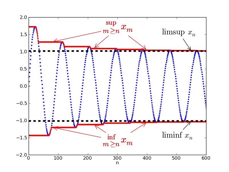
After
Front
ETH::2._Semester::Analysis::2._Folgen::3._Häufungspunkte::2._Limsup_und_Liminf
Die Größe \[ \limsup_{n \rightarrow \infty} a_n = {{c1:: \lim_{n \rightarrow \infty} \sup \{a_k \mid k \ge n \} }}\] heisst Limes superior der Folge \(a_n\).
Back
ETH::2._Semester::Analysis::2._Folgen::3._Häufungspunkte::2._Limsup_und_Liminf
Die Größe \[ \limsup_{n \rightarrow \infty} a_n = {{c1:: \lim_{n \rightarrow \infty} \sup \{a_k \mid k \ge n \} }}\] heisst Limes superior der Folge \(a_n\).
Das gleiche gilt für den Limes inferior.
Field-by-field Comparison
| Field |
Before |
After |
| Text |
Die Größe \[ \limsup_{n \rightarrow \infty} a_n = {{c1:: \lim_{n \rightarrow \infty} \sup \{a_k \mid k \ge n \} }}\] heißt <i>Limes superior</i> der Folge \(a_n\). |
Die Größe \[ \limsup_{n \rightarrow \infty} a_n = {{c1:: \lim_{n \rightarrow \infty} \sup \{a_k \mid k \ge n \} }}\] heisst <i>Limes superior</i> der Folge \(a_n\). |
Tags:
ETH::2._Semester::Analysis::2._Folgen::3._Häufungspunkte::2._Limsup_und_Liminf
Note 60: ETH::2. Semester::Analysis
Deck: ETH::2. Semester::Analysis
Note Type: Horvath Cloze
GUID: jKmAIMv))S
modified
Before
Front
ETH::2._Semester::Analysis::4._Funktionen::3._Grenzwerte
- Vertikale Asymptote -> Funktionswert gegen {{c2::\(\infty\) für \(x \to c \in \mathbb{R}\)}}
- Horizontale Asymptote -> Funktionswert gegen {{c2::\(c \in \mathbb{R}\) aber \(x \to \infty\)}}
Back
ETH::2._Semester::Analysis::4._Funktionen::3._Grenzwerte
- Vertikale Asymptote -> Funktionswert gegen {{c2::\(\infty\) für \(x \to c \in \mathbb{R}\)}}
- Horizontale Asymptote -> Funktionswert gegen {{c2::\(c \in \mathbb{R}\) aber \(x \to \infty\)}}
After
Front
ETH::2._Semester::Analysis::4._Funktionen::3._Grenzwerte
- Vertikale Asymptote \(\rightarrow\) Funktionswert gegen {{c2::\(\infty\) für \(x \to c \in \mathbb{R}\)}}
- Horizontale Asymptote \(\rightarrow\) Funktionswert gegen {{c2::\(c \in \mathbb{R}\), aber \(x \to \infty\)}}
Back
ETH::2._Semester::Analysis::4._Funktionen::3._Grenzwerte
- Vertikale Asymptote \(\rightarrow\) Funktionswert gegen {{c2::\(\infty\) für \(x \to c \in \mathbb{R}\)}}
- Horizontale Asymptote \(\rightarrow\) Funktionswert gegen {{c2::\(c \in \mathbb{R}\), aber \(x \to \infty\)}}
Field-by-field Comparison
| Field |
Before |
After |
| Text |
<ol><li>{{c1::Vertikale}} Asymptote -> Funktionswert gegen {{c2::\(\infty\) für \(x \to c \in \mathbb{R}\)}}</li><li>{{c1::Horizontale}} Asymptote -> Funktionswert gegen {{c2::\(c \in \mathbb{R}\) aber \(x \to \infty\)}}</li></ol> |
<ol><li>{{c1::Vertikale}} Asymptote \(\rightarrow\) Funktionswert gegen {{c2::\(\infty\) für \(x \to c \in \mathbb{R}\)}}</li><li>{{c1::Horizontale}} Asymptote \(\rightarrow\) Funktionswert gegen {{c2::\(c \in \mathbb{R}\), aber \(x \to \infty\)}}</li></ol> |
Tags:
ETH::2._Semester::Analysis::4._Funktionen::3._Grenzwerte
Note 61: ETH::2. Semester::Analysis
Deck: ETH::2. Semester::Analysis
Note Type: Horvath Classic
GUID: jKp`Sev.N*
modified
Before
Front
ETH::2._Semester::Analysis::2._Folgen::2._Konvergenz::4._Cauchy_Folge
Warum gilt Cauchy \(\iff\) konvergent in \(\mathbb{R}\), aber nicht in \(\mathbb{Q}\)?
Back
ETH::2._Semester::Analysis::2._Folgen::2._Konvergenz::4._Cauchy_Folge
Warum gilt Cauchy \(\iff\) konvergent in \(\mathbb{R}\), aber nicht in \(\mathbb{Q}\)?
In \(\mathbb{R}\): jede Cauchy-Folge konvergiert in \(\mathbb{R}\) (Vollständigkeit).
In \(\mathbb{Q}\): Eine Cauchy-Folge in \(\mathbb{Q}\) kann gegen \(\sqrt{2} \notin \mathbb{Q}\) konvergieren — der Grenzwert liegt außerhalb des Raumes. \(\mathbb{Q}\) ist nicht vollständig.
After
Front
ETH::2._Semester::Analysis::2._Folgen::2._Konvergenz::4._Cauchy_Folge
Warum ist jede Cauchy-Folge in \(\mathbb{R}\) konvergent, aber nicht jede in \(\mathbb{Q}\)?
Back
ETH::2._Semester::Analysis::2._Folgen::2._Konvergenz::4._Cauchy_Folge
Warum ist jede Cauchy-Folge in \(\mathbb{R}\) konvergent, aber nicht jede in \(\mathbb{Q}\)?
Weil \(\mathbb{R}\) vollständig ist (keine "Lücken"), während \(\mathbb{Q}\) das nicht ist.
Beispiel:
Die Folge \(1,\; 1.4,\; 1.41,\; 1.414,\; \dots\) ist Cauchy in \(\mathbb{Q}\), konvergiert aber gegen \(\sqrt{2} \notin \mathbb{Q}\).
Der Grenzwert existiert in \(\mathbb{Q}\) nicht - die "Lücke" fehlt.
In \(\mathbb{R}\) ist \(\sqrt{2}\) vorhanden, also konvergiert die Folge dort.
Field-by-field Comparison
| Field |
Before |
After |
| Front |
Warum gilt Cauchy \(\iff\) konvergent in \(\mathbb{R}\), aber nicht in \(\mathbb{Q}\)? |
Warum ist jede Cauchy-Folge in \(\mathbb{R}\) konvergent, aber nicht jede in \(\mathbb{Q}\)? |
| Back |
In \(\mathbb{R}\): jede Cauchy-Folge konvergiert <b>in</b> \(\mathbb{R}\) (Vollständigkeit).<br><br>In \(\mathbb{Q}\): Eine Cauchy-Folge in \(\mathbb{Q}\) kann gegen \(\sqrt{2} \notin \mathbb{Q}\) konvergieren — der Grenzwert liegt außerhalb des Raumes. \(\mathbb{Q}\) ist <b>nicht vollständig</b>. |
Weil \(\mathbb{R}\) vollständig ist (keine "Lücken"), während \(\mathbb{Q}\) das nicht ist.<br><br><b>Beispiel:</b><br>Die Folge \(1,\; 1.4,\; 1.41,\; 1.414,\; \dots\) ist Cauchy in \(\mathbb{Q}\), konvergiert aber gegen \(\sqrt{2} \notin \mathbb{Q}\).<br>Der Grenzwert existiert in \(\mathbb{Q}\) nicht - die "Lücke" fehlt.<br>In \(\mathbb{R}\) ist \(\sqrt{2}\) vorhanden, also konvergiert die Folge dort. |
Tags:
ETH::2._Semester::Analysis::2._Folgen::2._Konvergenz::4._Cauchy_Folge
Note 62: ETH::2. Semester::Analysis
Deck: ETH::2. Semester::Analysis
Note Type: Horvath Cloze
GUID: lH60#y9B27
modified
Before
Front
ETH::2._Semester::Analysis::4._Funktionen::3._Grenzwerte
Limes Definition: Wir können auch \(x_0\) als Argument ausschließen, in dem wir den Grenzwert anders definieren:
\[ \forall \epsilon > 0 \ \exists \delta > 0 \text{ so dass für alle } x \in \mathbb{D}(f)\] \[ 0 < |x - x_0| < \delta \implies | f(x) - L| < \epsilon \]
Back
ETH::2._Semester::Analysis::4._Funktionen::3._Grenzwerte
Limes Definition: Wir können auch \(x_0\) als Argument ausschließen, in dem wir den Grenzwert anders definieren:
\[ \forall \epsilon > 0 \ \exists \delta > 0 \text{ so dass für alle } x \in \mathbb{D}(f)\] \[ 0 < |x - x_0| < \delta \implies | f(x) - L| < \epsilon \]
Da gilt \(0 < |x - x_0|\) kann \(x\) nicht den Wert \(x_0\) annehmen.
After
Front
ETH::2._Semester::Analysis::4._Funktionen::3._Grenzwerte
Die alternative Grenzwertdefinition schliesst \(x_0\) selbst aus:
\[\begin{gathered}\forall \varepsilon > 0\;\exists \delta > 0 \text{ so dass für alle } x \in \mathbb{D}(f) \\ 0 < |x - x_0| < \delta \implies |f(x) - L| < \varepsilon\end{gathered}\]
Back
ETH::2._Semester::Analysis::4._Funktionen::3._Grenzwerte
Die alternative Grenzwertdefinition schliesst \(x_0\) selbst aus:
\[\begin{gathered}\forall \varepsilon > 0\;\exists \delta > 0 \text{ so dass für alle } x \in \mathbb{D}(f) \\ 0 < |x - x_0| < \delta \implies |f(x) - L| < \varepsilon\end{gathered}\]
Durch \(0 < |x - x_0|\) ist der Grenzwert unabhängig vom Funktionswert bei \(x_0\) - selbst wenn \(f(x_0)\) nicht definiert ist.
Da gilt \(0 < |x - x_0|\) kann \(x\) nicht den Wert \(x_0\) annehmen.
Field-by-field Comparison
| Field |
Before |
After |
| Text |
<b>Limes Definition: </b>Wir können auch \(x_0\) als Argument ausschließen, in dem wir den Grenzwert anders definieren:<br>\[ \forall \epsilon > 0 \ \exists \delta > 0 \text{ so dass für alle } x \in \mathbb{D}(f)\] \[{{c1:: 0 < |x - x_0| < \delta \implies | f(x) - L| < \epsilon }}\] |
Die <b>alternative Grenzwertdefinition</b> schliesst \(x_0\) selbst aus:<br>\[\begin{gathered}\forall \varepsilon > 0\;\exists \delta > 0 \text{ so dass für alle } x \in \mathbb{D}(f) \\ {{c1:: 0 < |x - x_0| < \delta \implies |f(x) - L| < \varepsilon}}\end{gathered}\] |
| Extra |
Da gilt \(0 < |x - x_0|\) kann \(x\) nicht den Wert \(x_0\) annehmen. |
Durch \(0 < |x - x_0|\) ist der Grenzwert unabhängig vom Funktionswert bei \(x_0\) - selbst wenn \(f(x_0)\) nicht definiert ist.<br><br>Da gilt \(0 < |x - x_0|\) kann \(x\) nicht den Wert \(x_0\) annehmen. |
Tags:
ETH::2._Semester::Analysis::4._Funktionen::3._Grenzwerte
Note 63: ETH::2. Semester::Analysis
Deck: ETH::2. Semester::Analysis
Note Type: Horvath Cloze
GUID: odE}
modified
Before
Front
ETH::2._Semester::Analysis::2._Folgen::2._Konvergenz::4._Cauchy_Folge
Eine Folge konvergiert \(\Longleftrightarrow\) sie {{c2:: eine Cauchy-Folge ist (für Folgen in \(\mathbb{R}\) und \(\mathbb{C}\))}}.
Back
ETH::2._Semester::Analysis::2._Folgen::2._Konvergenz::4._Cauchy_Folge
Eine Folge konvergiert \(\Longleftrightarrow\) sie {{c2:: eine Cauchy-Folge ist (für Folgen in \(\mathbb{R}\) und \(\mathbb{C}\))}}.
Dies gilt nicht für Folgen in \(\mathbb{Q}\), da sie zum Beispiel auf \(\sqrt{2}\) konvergieren können, was jedoch nicht in \(\mathbb{Q}\) liegt -> ergo konvergiert nie.
After
Front
ETH::2._Semester::Analysis::2._Folgen::2._Konvergenz::4._Cauchy_Folge
Eine Folge konvergiert \(\Longleftrightarrow\) Sie ist {{c2:: eine Cauchy-Folge (für Folgen in \(\mathbb{R}\) und \(\mathbb{C}\))}}.
Back
ETH::2._Semester::Analysis::2._Folgen::2._Konvergenz::4._Cauchy_Folge
Eine Folge konvergiert \(\Longleftrightarrow\) Sie ist {{c2:: eine Cauchy-Folge (für Folgen in \(\mathbb{R}\) und \(\mathbb{C}\))}}.
Dies gilt nicht für Folgen in \(\mathbb{Q}\), da sie zum Beispiel auf \(\sqrt{2}\) konvergieren können, was jedoch nicht in \(\mathbb{Q}\) liegt -> ergo konvergiert nie.
Field-by-field Comparison
| Field |
Before |
After |
| Text |
Eine Folge {{c1::<b>konvergiert</b>}} \(\Longleftrightarrow\) sie {{c2:: eine Cauchy-Folge ist (für Folgen in \(\mathbb{R}\) und \(\mathbb{C}\))}}. |
Eine Folge {{c1::<b>konvergiert</b>}} \(\Longleftrightarrow\) Sie ist {{c2:: eine Cauchy-Folge (für Folgen in \(\mathbb{R}\) und \(\mathbb{C}\))}}. |
Tags:
ETH::2._Semester::Analysis::2._Folgen::2._Konvergenz::4._Cauchy_Folge
Note 64: ETH::2. Semester::Analysis
Deck: ETH::2. Semester::Analysis
Note Type: Horvath Cloze
GUID: tRig1dAtan06
modified
Before
Front
ETH::2._Semester::Analysis::0._Trigonometrie::2._Identitäten::1._Arcostangens
The range of \(\arctan\) is \({{c1::\left(-\frac{\pi}{2},\, \frac{\pi}{2}\right)}}\), and it is a strictly increasing function.
Back
ETH::2._Semester::Analysis::0._Trigonometrie::2._Identitäten::1._Arcostangens
The range of \(\arctan\) is \({{c1::\left(-\frac{\pi}{2},\, \frac{\pi}{2}\right)}}\), and it is a strictly increasing function.
After
Front
ETH::2._Semester::Analysis::0._Trigonometrie::2._Identitäten::1._Arcostangens
Der Wertebereich von \(\arctan\) ist \({{c1::\left(-\frac{\pi}{2},\, \frac{\pi}{2}\right)}}\), und die Funktion ist streng monoton steigend.
Back
ETH::2._Semester::Analysis::0._Trigonometrie::2._Identitäten::1._Arcostangens
Der Wertebereich von \(\arctan\) ist \({{c1::\left(-\frac{\pi}{2},\, \frac{\pi}{2}\right)}}\), und die Funktion ist streng monoton steigend.
Field-by-field Comparison
| Field |
Before |
After |
| Text |
The range of \(\arctan\) is \({{c1::\left(-\frac{\pi}{2},\, \frac{\pi}{2}\right)}}\), and it is a {{c1::strictly increasing}} function. |
Der Wertebereich von \(\arctan\) ist \({{c1::\left(-\frac{\pi}{2},\, \frac{\pi}{2}\right)}}\), und die Funktion ist {{c1::streng monoton steigend::Wachstumsverhalten}}. |
Tags:
ETH::2._Semester::Analysis::0._Trigonometrie::2._Identitäten::1._Arcostangens
Note 65: ETH::2. Semester::Analysis
Deck: ETH::2. Semester::Analysis
Note Type: Horvath Cloze
GUID: tRig1dPyth01
modified
Before
Front
ETH::2._Semester::Analysis::0._Trigonometrie::2._Identitäten::3._Pythagoras
\[ \sin^2\theta + \cos^2\theta = 1 \]
Back
ETH::2._Semester::Analysis::0._Trigonometrie::2._Identitäten::3._Pythagoras
\[ \sin^2\theta + \cos^2\theta = 1 \]
After
Front
ETH::2._Semester::Analysis::0._Trigonometrie::2._Identitäten::3._Pythagoras
\[ {{c1::\sin^2\theta + \cos^2\theta :: \text{Identity} }} = 1 \]
Back
ETH::2._Semester::Analysis::0._Trigonometrie::2._Identitäten::3._Pythagoras
\[ {{c1::\sin^2\theta + \cos^2\theta :: \text{Identity} }} = 1 \]
Field-by-field Comparison
| Field |
Before |
After |
| Text |
\[ {{c1::\sin^2\theta + \cos^2\theta :: Identity }} = {{c2::1}} \] |
\[ {{c1::\sin^2\theta + \cos^2\theta :: \text{Identity} }} = {{c2::1}} \] |
Tags:
ETH::2._Semester::Analysis::0._Trigonometrie::2._Identitäten::3._Pythagoras
Note 66: ETH::2. Semester::Analysis
Deck: ETH::2. Semester::Analysis
Note Type: Horvath Cloze
GUID: u$3f,(&]?[
modified
Before
Front
ETH::2._Semester::Analysis::3._Reihen::1._Definitionen
Absolut konvergent \(\implies\) konvergent
Back
ETH::2._Semester::Analysis::3._Reihen::1._Definitionen
Absolut konvergent \(\implies\) konvergent
nicht andersherum
After
Front
ETH::2._Semester::Analysis::3._Reihen::1._Definitionen
Absolut konvergent \(\implies\)konvergent
Back
ETH::2._Semester::Analysis::3._Reihen::1._Definitionen
Absolut konvergent \(\implies\)konvergent
nicht andersherum, na no na ned
Field-by-field Comparison
| Field |
Before |
After |
| Text |
Absolut konvergent \(\implies\) {{c2::konvergent}} |
Absolut konvergent \(\implies\){{c1::konvergent}} |
| Extra |
nicht andersherum |
nicht andersherum, na no na ned |
Tags:
ETH::2._Semester::Analysis::3._Reihen::1._Definitionen
Note 67: ETH::2. Semester::Analysis
Deck: ETH::2. Semester::Analysis
Note Type: Horvath Cloze
GUID: w)NK`}V9nz
modified
Before
Front
ETH::2._Semester::Analysis::3._Reihen::3._Konvergenzkriterien
Falls \(\sum a_n\) konvergiert, dann gilt zwingend: \(\lim_{n\to\infty} a_n = 0\).
Back
ETH::2._Semester::Analysis::3._Reihen::3._Konvergenzkriterien
Falls \(\sum a_n\) konvergiert, dann gilt zwingend: \(\lim_{n\to\infty} a_n = 0\).
Gegenbeispiel: harmonische Reihe \(\sum 1/n\)
After
Front
ETH::2._Semester::Analysis::3._Reihen::3._Konvergenzkriterien
Falls \(\sum a_n\) konvergiert, dann gilt zwingend, dass \(\lim_{n\to\infty} a_n = 0\).
Back
ETH::2._Semester::Analysis::3._Reihen::3._Konvergenzkriterien
Falls \(\sum a_n\) konvergiert, dann gilt zwingend, dass \(\lim_{n\to\infty} a_n = 0\).
Gilt jedoch nicht in die andere Richtung, siehe z.B. die harmonische Reihe \(\sum 1/n\).
Field-by-field Comparison
| Field |
Before |
After |
| Text |
Falls \(\sum a_n\) konvergiert, dann gilt zwingend: \(\lim_{n\to\infty} a_n = {{c1::0}}\). |
Falls \(\sum a_n\) konvergiert, dann gilt zwingend, dass \(\lim_{n\to\infty} a_n = {{c1::0}}\). |
| Extra |
Gegenbeispiel: harmonische Reihe \(\sum 1/n\) |
Gilt jedoch nicht in die andere Richtung, siehe z.B. die harmonische Reihe \(\sum 1/n\). |
Tags:
ETH::2._Semester::Analysis::3._Reihen::3._Konvergenzkriterien
Note 68: ETH::2. Semester::Analysis
Deck: ETH::2. Semester::Analysis
Note Type: Horvath Cloze
GUID: z>(#?Mm:.A
modified
Before
Front
ETH::2._Semester::Analysis::3._Reihen::1._Definitionen
Wenn \(\sum^\infty a_n\) konvergent ist gilt:
\[ \sum_{n = 0}^\infty a_n = {{c1::\sum_{n = 0}^{N - 1} + \sum_{n = N}^\infty a_n:: \text{split sum} }}\]
Back
ETH::2._Semester::Analysis::3._Reihen::1._Definitionen
Wenn \(\sum^\infty a_n\) konvergent ist gilt:
\[ \sum_{n = 0}^\infty a_n = {{c1::\sum_{n = 0}^{N - 1} + \sum_{n = N}^\infty a_n:: \text{split sum} }}\]
After
Front
ETH::2._Semester::Analysis::3._Reihen::1._Definitionen
Wenn \(\sum^\infty a_n\) konvergent ist, gilt:
\[ \sum_{n = 0}^\infty a_n = {{c1::\sum_{n = 0}^{N - 1} a_n + \sum_{n = N}^\infty a_n:: \text{split sum} }}\]
Back
ETH::2._Semester::Analysis::3._Reihen::1._Definitionen
Wenn \(\sum^\infty a_n\) konvergent ist, gilt:
\[ \sum_{n = 0}^\infty a_n = {{c1::\sum_{n = 0}^{N - 1} a_n + \sum_{n = N}^\infty a_n:: \text{split sum} }}\]
Field-by-field Comparison
| Field |
Before |
After |
| Text |
Wenn \(\sum^\infty a_n\) konvergent ist gilt:<br>\[ \sum_{n = 0}^\infty a_n = {{c1::\sum_{n = 0}^{N - 1} + \sum_{n = N}^\infty a_n:: \text{split sum} }}\] |
Wenn \(\sum^\infty a_n\) konvergent ist, gilt:<br>\[ \sum_{n = 0}^\infty a_n = {{c1::\sum_{n = 0}^{N - 1} a_n + \sum_{n = N}^\infty a_n:: \text{split sum} }}\] |
Tags:
ETH::2._Semester::Analysis::3._Reihen::1._Definitionen
Note 69: ETH::2. Semester::Analysis
Deck: ETH::2. Semester::Analysis
Note Type: Horvath Cloze
GUID: {XU$eYR/n`
modified
Before
Front
ETH::2._Semester::Analysis::3._Reihen::3._Konvergenzkriterien
Sei \(0 \leq a_n \leq b_n\) für alle \(n \geq N\):
\(\sum b_n\) konvergiert \(\implies \sum a_n \text{ konvergiert}\) (Majorante)
\(\sum a_n\) divergiert \(\implies \sum b_n \text{ divergiert}\) (Minorante)
Back
ETH::2._Semester::Analysis::3._Reihen::3._Konvergenzkriterien
Sei \(0 \leq a_n \leq b_n\) für alle \(n \geq N\):
\(\sum b_n\) konvergiert \(\implies \sum a_n \text{ konvergiert}\) (Majorante)
\(\sum a_n\) divergiert \(\implies \sum b_n \text{ divergiert}\) (Minorante)
Proof:
Da \(\sum_{n=1}^{\infty} b_n\) konvergiert, konvergiert die Folge der Partialsummen. Deswegen ist sie auch beschränkt.
Da alle \(a_k \le b_k\), gilt auch \(S_n \le T_n\) (\(S_n\) Partialsummen von \(\sum a_N\), \(T_n\) Partialsummen von \(\sum b_n\))
Dadurch ist auch \(S_n\) beschränkt und da sie monoton steigt (\(a_n \ge 0\)) ist sie auch konvergent. Dadurch ist \(\sum_{n=1}^{\infty} a_n\) konvergent.
After
Front
ETH::2._Semester::Analysis::3._Reihen::3._Konvergenzkriterien
Sei \(0 \leq a_n \leq b_n\) für alle \(n \geq N\):
\(\sum b_n\) konvergiert \(\implies \sum a_n\) konvergiert (Majorante)
\(\sum a_n\) divergiert \(\implies \sum b_n\) divergiert (Minorante)
Back
ETH::2._Semester::Analysis::3._Reihen::3._Konvergenzkriterien
Sei \(0 \leq a_n \leq b_n\) für alle \(n \geq N\):
\(\sum b_n\) konvergiert \(\implies \sum a_n\) konvergiert (Majorante)
\(\sum a_n\) divergiert \(\implies \sum b_n\) divergiert (Minorante)
Proof:
Da \(\sum_{n=1}^{\infty} b_n\) konvergiert, konvergiert die Folge der Partialsummen. Deswegen ist sie auch beschränkt.
Da alle \(a_k \le b_k\), gilt auch \(S_n \le T_n\) (\(S_n\) Partialsummen von \(\sum a_N\), \(T_n\) Partialsummen von \(\sum b_n\))
Dadurch ist auch \(S_n\) beschränkt und da sie monoton steigt (\(a_n \ge 0\)) ist sie auch konvergent. Dadurch ist \(\sum_{n=1}^{\infty} a_n\) konvergent.
Field-by-field Comparison
| Field |
Before |
After |
| Text |
Sei \(0 \leq a_n \leq b_n\) für alle \(n \geq N\):<br><br>\(\sum b_n\) konvergiert \(\implies {{c1::\sum a_n \text{ konvergiert}}}\) (<b>Majorante</b>)<br>\(\sum a_n\) divergiert \(\implies {{c2::\sum b_n \text{ divergiert}}}\) (<b>Minorante</b>) |
Sei \(0 \leq a_n \leq b_n\) für alle \(n \geq N\):<br><br>\(\sum b_n\) konvergiert \(\implies \sum a_n\) {{c1:: konvergiert (Majorante)}}<br>\(\sum a_n\) divergiert \(\implies \sum b_n\) {{c1::divergiert (Minorante)}} |
Tags:
ETH::2._Semester::Analysis::3._Reihen::3._Konvergenzkriterien
Note 70: ETH::2. Semester::Analysis
Deck: ETH::2. Semester::Analysis
Note Type: Horvath Cloze
GUID: {].oPsIfG|
modified
Before
Front
ETH::2._Semester::Analysis::3._Reihen::2._Standard_Reihen
Exponentialreihe:\[\exp(z) = {{c1:: \sum_{n=0}^\infty \frac{z^n}{n!} }}\]
Diese Reihe konvergiert {{c1::absolut für alle \(z \in \mathbb{C}\)}} (Konvergenzradius \(R = \infty\)).
Back
ETH::2._Semester::Analysis::3._Reihen::2._Standard_Reihen
Exponentialreihe:\[\exp(z) = {{c1:: \sum_{n=0}^\infty \frac{z^n}{n!} }}\]
Diese Reihe konvergiert {{c1::absolut für alle \(z \in \mathbb{C}\)}} (Konvergenzradius \(R = \infty\)).
After
Front
ETH::2._Semester::Analysis::3._Reihen::2._Standard_Reihen
Exponentialreihe:\[\exp(z) = {{c1:: \sum_{n=0}^\infty \frac{z^n}{n!} }}\]Diese Reihe konvergiert {{c2::absolut für alle \(z \in \mathbb{C}\)::Konvergenztyp}}.
Back
ETH::2._Semester::Analysis::3._Reihen::2._Standard_Reihen
Exponentialreihe:\[\exp(z) = {{c1:: \sum_{n=0}^\infty \frac{z^n}{n!} }}\]Diese Reihe konvergiert {{c2::absolut für alle \(z \in \mathbb{C}\)::Konvergenztyp}}.
(Konvergenzradius \(R = \infty\))
Field-by-field Comparison
| Field |
Before |
After |
| Text |
Exponentialreihe:\[\exp(z) = {{c1:: \sum_{n=0}^\infty \frac{z^n}{n!} }}\]<br>Diese Reihe konvergiert {{c1::absolut für alle \(z \in \mathbb{C}\)}} (Konvergenzradius \(R = \infty\)). |
Exponentialreihe:\[\exp(z) = {{c1:: \sum_{n=0}^\infty \frac{z^n}{n!} }}\]Diese Reihe konvergiert {{c2::absolut für alle \(z \in \mathbb{C}\)::Konvergenztyp}}. |
| Extra |
|
(Konvergenzradius \(R = \infty\)) |
Tags:
ETH::2._Semester::Analysis::3._Reihen::2._Standard_Reihen
Note 71: ETH::2. Semester::Analysis
Deck: ETH::2. Semester::Analysis
Note Type: Horvath Cloze
GUID: }3LSktDYts
modified
Before
Front
ETH::2._Semester::Analysis::3._Reihen::2._Standard_Reihen
Die Riemansche-Zeta Funktion Reihe \(\displaystyle\zeta(s) = {{c1:: \sum_{n=1}^\infty \frac{1}{n^s} }}\) konvergiert für \(s > 1\) und divergiert für \(s\leq1\).
Back
ETH::2._Semester::Analysis::3._Reihen::2._Standard_Reihen
Die Riemansche-Zeta Funktion Reihe \(\displaystyle\zeta(s) = {{c1:: \sum_{n=1}^\infty \frac{1}{n^s} }}\) konvergiert für \(s > 1\) und divergiert für \(s\leq1\).
Oft als Referenzreihe im Vergleichssatz nützlich (wenn Wurzel/Quotient versagen).
After
Front
ETH::2._Semester::Analysis::3._Reihen::2._Standard_Reihen
Die Riemansche-Zeta Funktion Reihe \(\displaystyle\zeta(s) = {{c1:: \sum_{n=1}^\infty \frac{1}{n^s} }}\) konvergiert für \(s > 1\) und divergiert für \(s\leq1\).
Back
ETH::2._Semester::Analysis::3._Reihen::2._Standard_Reihen
Die Riemansche-Zeta Funktion Reihe \(\displaystyle\zeta(s) = {{c1:: \sum_{n=1}^\infty \frac{1}{n^s} }}\) konvergiert für \(s > 1\) und divergiert für \(s\leq1\).
Oft als Referenzreihe im Vergleichssatz nützlich (wenn Wurzel/Quotient versagen).
Field-by-field Comparison
| Field |
Before |
After |
| Text |
Die Riemansche-Zeta Funktion Reihe \(\displaystyle\zeta(s) = {{c1:: \sum_{n=1}^\infty \frac{1}{n^s} }}\) konvergiert für {{c1::\(s > 1\)}} und divergiert für {{c1::\(s\leq1\)}}. |
Die Riemansche-Zeta Funktion Reihe \(\displaystyle\zeta(s) = {{c1:: \sum_{n=1}^\infty \frac{1}{n^s} }}\) konvergiert für {{c2::\(s > 1\)}} und divergiert für {{c2::\(s\leq1\)}}. |
Tags:
ETH::2._Semester::Analysis::3._Reihen::2._Standard_Reihen
Note 72: ETH::2. Semester::DDCA
Deck: ETH::2. Semester::DDCA
Note Type: Horvath Cloze
GUID: PMc1ViG{^J
modified
Before
Front
ETH::2._Semester::DDCA::04a._Sequential_Logic_Design_II_&_Finite_State_Machines::01._Sequential_Logic_Circuits
Most modern computers are synchronous "machines"
Back
ETH::2._Semester::DDCA::04a._Sequential_Logic_Design_II_&_Finite_State_Machines::01._Sequential_Logic_Circuits
Most modern computers are synchronous "machines"
State transitions take place at fixed units of time (i.e., potentially delayed response to input, synchronized to an external signal).
Controlled in part by a clock, as we will see soon.
After
Front
ETH::2._Semester::DDCA::04a._Sequential_Logic_Design_II_&_Finite_State_Machines::01._Sequential_Logic_Circuits
Most modern computers are synchronous "machines".
Back
ETH::2._Semester::DDCA::04a._Sequential_Logic_Design_II_&_Finite_State_Machines::01._Sequential_Logic_Circuits
Most modern computers are synchronous "machines".
State transitions take place at fixed units of time (i.e., potentially delayed response to input, synchronized to an external signal).
Controlled in part by a clock, as we will see soon.
Field-by-field Comparison
| Field |
Before |
After |
| Text |
Most modern computers are {{c1::synchronous}} "machines" |
Most modern computers are {{c1::synchronous}} "machines". |
Tags:
ETH::2._Semester::DDCA::04a._Sequential_Logic_Design_II_&_Finite_State_Machines::01._Sequential_Logic_Circuits
Note 73: ETH::2. Semester::PProg
Deck: ETH::2. Semester::PProg
Note Type: Horvath Cloze
GUID: ?aiVa43NDU
modified
Before
Front
ETH::2._Semester::PProg::10._Parallel_Algorithms::2._Parallel_patterns
Summing an array of n elements in parallel has work \(O(n)\), span \(O(\log n)\), and parallelism \(O(n / \log n)\).
Back
ETH::2._Semester::PProg::10._Parallel_Algorithms::2._Parallel_patterns
Summing an array of n elements in parallel has work \(O(n)\), span \(O(\log n)\), and parallelism \(O(n / \log n)\).
Work = \(O(n)\) (same as sequential).
Span = \(O(\log n)\) (tree depth).
Parallelism = work/span = \(O(n/\log n)\), meaning you benefit from up to \(O(n/\log n)\) processors before hitting the span bottleneck.
After
Front
ETH::2._Semester::PProg::10._Parallel_Algorithms::2._Parallel_patterns
Summing an array of \(n\) elements in parallel has work \(O(n)\), span \(O(\log n)\), and parallelism \(O(n / \log n)\).
Back
ETH::2._Semester::PProg::10._Parallel_Algorithms::2._Parallel_patterns
Summing an array of \(n\) elements in parallel has work \(O(n)\), span \(O(\log n)\), and parallelism \(O(n / \log n)\).
Work = \(O(n)\) (same as sequential).
Span = \(O(\log n)\) (tree depth).
Parallelism = work/span = \(O(n/\log n)\), meaning you benefit from up to \(O(n/\log n)\) processors before hitting the span bottleneck.
Field-by-field Comparison
| Field |
Before |
After |
| Text |
Summing an array of n elements in parallel has work \(O({{c1::n}})\), span \(O({{c2::\log n}})\), and parallelism \(O({{c3::n / \log n}})\). |
Summing an array of \(n\) elements in parallel has work \(O({{c1::n}})\), span \(O({{c2::\log n}})\), and parallelism \(O({{c3::n / \log n}})\). |
Tags:
ETH::2._Semester::PProg::10._Parallel_Algorithms::2._Parallel_patterns
Note 74: ETH::2. Semester::PProg
Deck: ETH::2. Semester::PProg
Note Type: Horvath Cloze
GUID: EdVyAbz-qv
modified
Before
Front
ETH::2._Semester::PProg::12._Shared_Memory_Concurrency
AtomicInteger provides atomic compound operations such as getAndIncrement() and compareAndSet(expected, update) without requiring synchronized.
Back
ETH::2._Semester::PProg::12._Shared_Memory_Concurrency
AtomicInteger provides atomic compound operations such as getAndIncrement() and compareAndSet(expected, update) without requiring synchronized.
Implemented via hardware CAS (compare-and-swap). Faster than synchronized for simple counters. Part of java.util.concurrent.atomic.
After
Front
ETH::2._Semester::PProg::12._Shared_Memory_Concurrency
AtomicInteger provides atomic compound operations such as getAndIncrement() and compareAndSet(expected, update) without requiring synchronized.
Back
ETH::2._Semester::PProg::12._Shared_Memory_Concurrency
AtomicInteger provides atomic compound operations such as getAndIncrement() and compareAndSet(expected, update) without requiring synchronized.
Faster than synchronized for simple counters.
Implemented via hardware CAS (compare-and-swap).
Part of java.util.concurrent.atomic.
Field-by-field Comparison
| Field |
Before |
After |
| Text |
<code>{{c1::AtomicInteger}}</code> provides {{c2::atomic compound operations}} such as <code>{{c2::getAndIncrement()}}</code> and <code>{{c2::compareAndSet(expected, update)}}</code> without requiring <code>synchronized</code>. |
<code>{{c1::AtomicInteger}}</code> provides {{c2::atomic compound operations such as <code>getAndIncrement()</code> and <code>compareAndSet(expected, update)}}</code> without requiring <code>synchronized</code>. |
| Extra |
Implemented via hardware CAS (compare-and-swap). Faster than <code>synchronized</code> for simple counters. Part of <code>java.util.concurrent.atomic</code>. |
Faster than <code>synchronized</code> for simple counters.<br><br>Implemented via hardware CAS (compare-and-swap).<br><br>Part of <code>java.util.concurrent.atomic</code>. |
Tags:
ETH::2._Semester::PProg::12._Shared_Memory_Concurrency
Note 75: ETH::2. Semester::PProg
Deck: ETH::2. Semester::PProg
Note Type: Horvath Cloze
GUID: GH&YPQRsTh
modified
Before
Front
ETH::2._Semester::PProg::06._Parallel_Architecture::3._Pipelining
Lead-in and lead-out reduce effective throughput below the theoretical bound for a finite number of elements \(N\). Their impact is largest when \(N\) is small (short pipelines).
Back
ETH::2._Semester::PProg::06._Parallel_Architecture::3._Pipelining
Lead-in and lead-out reduce effective throughput below the theoretical bound for a finite number of elements \(N\). Their impact is largest when \(N\) is small (short pipelines).
Example: for a finite run, effective throughput was 0.7 while the infinite-stream bound was 1. As N → ∞, effective throughput approaches 1/max(stage_time).
After
Front
ETH::2._Semester::PProg::06._Parallel_Architecture::3._Pipelining
Lead-in and lead-out reduce effective throughput below the theoretical bound for a finite number of elements \(N\).
Their impact is largest when \(N\) is small (short pipelines).
Back
ETH::2._Semester::PProg::06._Parallel_Architecture::3._Pipelining
Lead-in and lead-out reduce effective throughput below the theoretical bound for a finite number of elements \(N\).
Their impact is largest when \(N\) is small (short pipelines).
Example:
For a finite run, effective throughput was 0.7 while the infinite-stream bound was 1. As N → ∞, effective throughput approaches 1/max(stage_time).
Field-by-field Comparison
| Field |
Before |
After |
| Text |
Lead-in and lead-out {{c1::reduce effective throughput below the theoretical bound}} for {{c2::a finite number of elements \(N\)}}. Their impact is largest when {{c3::\(N\) is small (short pipelines)}}. |
Lead-in and lead-out reduce {{c1::effective throughput below the theoretical bound}} for {{c2::a finite number of elements \(N\)}}. <br><br>Their impact is largest when {{c3::\(N\) is small (short pipelines)}}. |
| Extra |
Example: for a finite run, effective throughput was 0.7 while the infinite-stream bound was 1. As N → ∞, effective throughput approaches 1/max(stage_time). |
<b>Example:</b> <br>For a finite run, effective throughput was 0.7 while the infinite-stream bound was 1. As N → ∞, effective throughput approaches 1/max(stage_time). |
Tags:
ETH::2._Semester::PProg::06._Parallel_Architecture::3._Pipelining
Note 76: ETH::2. Semester::PProg
Deck: ETH::2. Semester::PProg
Note Type: Horvath Classic
GUID: KD1&||&6xW
modified
Before
Front
ETH::2._Semester::PProg::10._Parallel_Algorithms::1._Task_graphs_and_performance_measures
Why is \(T_p \geq T_1/p\) a strict lower bound — why can no scheduler beat it?
Back
ETH::2._Semester::PProg::10._Parallel_Algorithms::1._Task_graphs_and_performance_measures
Why is \(T_p \geq T_1/p\) a strict lower bound — why can no scheduler beat it?
\(T_1\) is the total work (sum of all node costs in the DAG).
With \(p\) processors, at most \(p\) units of work can be done per time step.
herefore the minimum time to do \(T_1\) units of work is \(T_1/p\).
This is a counting argument, independent of the scheduler's strategy.
After
Front
ETH::2._Semester::PProg::10._Parallel_Algorithms::1._Task_graphs_and_performance_measures
Why is \(T_p \geq T_1/p\) a strict lower bound - why can no scheduler beat it?
Back
ETH::2._Semester::PProg::10._Parallel_Algorithms::1._Task_graphs_and_performance_measures
Why is \(T_p \geq T_1/p\) a strict lower bound - why can no scheduler beat it?
\(T_1\) is the total work (sum of all node costs in the DAG).
With \(p\) processors, at most \(p\) units of work can be done per time step.
Therefore the minimum time to do \(T_1\) units of work is \(T_1/p\).
This is a counting argument, independent of the scheduler's strategy.
Field-by-field Comparison
| Field |
Before |
After |
| Front |
Why is \(T_p \geq T_1/p\) a strict lower bound — why can no scheduler beat it? |
Why is \(T_p \geq T_1/p\) a strict lower bound - why can no scheduler beat it? |
| Back |
\(T_1\) is the total work (sum of all node costs in the DAG). <br>With \(p\) processors, at most \(p\) units of work can be done per time step. <br>herefore the minimum time to do \(T_1\) units of work is \(T_1/p\).<br><br>This is a counting argument, independent of the scheduler's strategy. |
\(T_1\) is the total work (sum of all node costs in the DAG). <br>With \(p\) processors, at most \(p\) units of work can be done per time step. <br>Therefore the minimum time to do \(T_1\) units of work is \(T_1/p\).<br><br>This is a counting argument, independent of the scheduler's strategy. |
Tags:
ETH::2._Semester::PProg::10._Parallel_Algorithms::1._Task_graphs_and_performance_measures
Note 77: ETH::2. Semester::PProg
Deck: ETH::2. Semester::PProg
Note Type: Horvath Classic
GUID: KqO7gK}Fu/
modified
Before
Front
ETH::2._Semester::PProg::05._Java_Threads::3._Wait,_Notify,_NotifyAll
When should you prefer notifyAll() over notify()?
Back
ETH::2._Semester::PProg::05._Java_Threads::3._Wait,_Notify,_NotifyAll
When should you prefer notifyAll() over notify()?
Prefer notifyAll() when multiple threads may be waiting and they have different conditions to wait for. notify() wakes only one (arbitrary) thread — if it wakes a thread whose condition is still false, it goes back to sleep and no progress is made. notifyAll() wakes all waiters; each re-checks its condition in its while loop. Cost: more context switches. Safe default: always use notifyAll() unless you have a single-condition, single-consumer pattern.
After
Front
ETH::2._Semester::PProg::05._Java_Threads::3._Wait,_Notify,_NotifyAll
When should you prefer notifyAll() over notify()?
Back
ETH::2._Semester::PProg::05._Java_Threads::3._Wait,_Notify,_NotifyAll
When should you prefer notifyAll() over notify()?
When multiple threads may be waiting and they have different conditions to wait for.
notify()
notifyAll()while loop.
Cost: more context switches.
Safe default: always use notifyAll() unless you have a single-condition, single-consumer pattern.
Field-by-field Comparison
| Field |
Before |
After |
| Front |
When should you prefer <code>notifyAll()</code> over <code>notify()</code>? |
When should you prefer <code>notifyAll()</code> over <code>notify()</code>? |
| Back |
Prefer <code>notifyAll()</code> when <b>multiple threads</b> may be waiting and they have <b>different conditions</b> to wait for. <code>notify()</code> wakes only one (arbitrary) thread — if it wakes a thread whose condition is still false, it goes back to sleep and no progress is made. <code>notifyAll()</code> wakes all waiters; each re-checks its condition in its <code>while</code> loop. Cost: more context switches. Safe default: always use <code>notifyAll()</code> unless you have a single-condition, single-consumer pattern. |
When <b>multiple threads</b> may be waiting and they have <b>different conditions</b> to wait for. <br><code><br>notify()</code> wakes only one (arbitrary) thread - if it wakes a thread whose condition is still false, it goes back to sleep and no progress is made.<code><br>notifyAll()</code> wakes all waiters; each re-checks its condition in its <code>while</code> loop. <br><br>Cost: more context switches. <br>Safe default: always use <code>notifyAll()</code> unless you have a single-condition, single-consumer pattern. |
Tags:
ETH::2._Semester::PProg::05._Java_Threads::3._Wait,_Notify,_NotifyAll
Note 78: ETH::2. Semester::PProg
Deck: ETH::2. Semester::PProg
Note Type: Horvath Classic
GUID: Lj=X5W/02X
modified
Before
Front
ETH::2._Semester::PProg::10._Parallel_Algorithms::3._Parallel_algorithms
What does each node store after the up pass (reduce pass) of the parallel prefix-sum algorithm?
Back
ETH::2._Semester::PProg::10._Parallel_Algorithms::3._Parallel_algorithms
What does each node store after the up pass (reduce pass) of the parallel prefix-sum algorithm?
Each internal node stores the sum of all leaves in its subtree. Leaves store the original values. This pass is a parallel tree reduction — done bottom-up with O(n) work and O(log n) span.
After
Front
ETH::2._Semester::PProg::10._Parallel_Algorithms::3._Parallel_algorithms
What does each node store after the up pass (reduce pass) of the parallel prefix-sum algorithm?
Back
ETH::2._Semester::PProg::10._Parallel_Algorithms::3._Parallel_algorithms
What does each node store after the up pass (reduce pass) of the parallel prefix-sum algorithm?
The sum of all leaves in its subtree.
Leaves store the original values.
This pass is a parallel tree reduction - done bottom-up with \(O(n)\) work and \(O(\log n)\) span.
Field-by-field Comparison
| Field |
Before |
After |
| Back |
Each internal node stores the <b>sum of all leaves in its subtree</b>. Leaves store the original values. This pass is a parallel tree reduction — done bottom-up with O(n) work and O(log n) span. |
The sum of all leaves in its subtree. <br><br>Leaves store the original values.<br>This pass is a parallel tree reduction - done bottom-up with \(O(n)\) work and \(O(\log n)\) span. |
Tags:
ETH::2._Semester::PProg::10._Parallel_Algorithms::3._Parallel_algorithms
Note 79: ETH::2. Semester::PProg
Deck: ETH::2. Semester::PProg
Note Type: Horvath Cloze
GUID: NLVo5v1@Dy
modified
Before
Front
ETH::2._Semester::PProg::10._Parallel_Algorithms::3._Parallel_algorithms
Pack (also called filter) takes a collection and a predicate and returns a new array containing only the elements satisfying the predicate, preserving their original relative order.
Back
ETH::2._Semester::PProg::10._Parallel_Algorithms::3._Parallel_algorithms
Pack (also called filter) takes a collection and a predicate and returns a new array containing only the elements satisfying the predicate, preserving their original relative order.
Example: pack([3,1,4,1,5], x > 2) → [3,4,5]. This is the parallel equivalent of a sequential filter loop.
After
Front
ETH::2._Semester::PProg::10._Parallel_Algorithms::3._Parallel_algorithms
Pack (also called filter) takes a collection and a predicate and returns a new array containing only the elements satisfying the predicate, preserving their original relative order.
Back
ETH::2._Semester::PProg::10._Parallel_Algorithms::3._Parallel_algorithms
Pack (also called filter) takes a collection and a predicate and returns a new array containing only the elements satisfying the predicate, preserving their original relative order.
Example:
pack([3,1,4,1,5], x > 2) → [3,4,5].
This is the parallel equivalent of a sequential filter loop.
Field-by-field Comparison
| Field |
Before |
After |
| Text |
{{c1::Pack}} (also called filter) takes a collection and a predicate and returns {{c2::a new array containing only the elements satisfying the predicate, preserving their original relative order}}. |
{{c1::Pack (also called filter)}} takes a collection and a predicate and returns {{c2::a new array containing only the elements satisfying the predicate, preserving their original relative order}}. |
| Extra |
Example: pack([3,1,4,1,5], x > 2) → [3,4,5]. This is the parallel equivalent of a sequential filter loop. |
<b>Example:</b> <br>pack([3,1,4,1,5], x > 2) → [3,4,5]. <br>This is the parallel equivalent of a sequential filter loop. |
Tags:
ETH::2._Semester::PProg::10._Parallel_Algorithms::3._Parallel_algorithms
Note 80: ETH::2. Semester::PProg
Deck: ETH::2. Semester::PProg
Note Type: Horvath Classic
GUID: OG4szVeI~<
modified
Before
Front
ETH::2._Semester::PProg::10._Parallel_Algorithms::3._Parallel_algorithms
Why does parallel prefix sum require two passes (up then down) rather than one?
Back
ETH::2._Semester::PProg::10._Parallel_Algorithms::3._Parallel_algorithms
Why does parallel prefix sum require two passes (up then down) rather than one?
The up-sweep computes partial sums in a tree structure, but each node only knows the sum of its subtree - not the sum of all elements to its left.
The down-sweep propagates these missing left-side contributions back down the tree, so that every position ends up with the correct prefix sum.
After
Front
ETH::2._Semester::PProg::10._Parallel_Algorithms::3._Parallel_algorithms
Why does parallel prefix sum require two passes (up then down), rather than one?
Back
ETH::2._Semester::PProg::10._Parallel_Algorithms::3._Parallel_algorithms
Why does parallel prefix sum require two passes (up then down), rather than one?
The up-sweep computes partial sums in a tree structure, but each node only knows the sum of its subtree - not the sum of all elements to its left.
The down-sweep propagates these missing left-side contributions back down the tree, so that every position ends up with the correct prefix sum.
Field-by-field Comparison
| Field |
Before |
After |
| Front |
Why does parallel prefix sum require two passes (up then down) rather than one? |
Why does parallel prefix sum require two passes (up then down), rather than one? |
Tags:
ETH::2._Semester::PProg::10._Parallel_Algorithms::3._Parallel_algorithms
Note 81: ETH::2. Semester::PProg
Deck: ETH::2. Semester::PProg
Note Type: Horvath Cloze
GUID: XZFu@~1-gN
modified
Before
Front
ETH::2._Semester::PProg::05._Java_Threads::3._Wait,_Notify,_NotifyAll
After calling notifyAll(), the calling thread does not release the lock immediately, it only releases it when it exits the synchronized block or calls wait().
Back
ETH::2._Semester::PProg::05._Java_Threads::3._Wait,_Notify,_NotifyAll
After calling notifyAll(), the calling thread does not release the lock immediately, it only releases it when it exits the synchronized block or calls wait().
All woken threads move to RUNNABLE state and compete for the lock, but only one can acquire it at a time. The notifying thread still holds the lock until it finishes its synchronized section.
After
Front
ETH::2._Semester::PProg::05._Java_Threads::3._Wait,_Notify,_NotifyAll
After calling notifyAll(), the calling thread does not release the lock immediately, it only releases it when it exits the synchronized block or calls wait().
Back
ETH::2._Semester::PProg::05._Java_Threads::3._Wait,_Notify,_NotifyAll
After calling notifyAll(), the calling thread does not release the lock immediately, it only releases it when it exits the synchronized block or calls wait().
All woken threads move to RUNNABLE state and compete for the lock, but only one can acquire it at a time. The notifying thread still holds the lock until it finishes its synchronized section.
Field-by-field Comparison
| Field |
Before |
After |
| Text |
After calling <code>notifyAll()</code>, the calling thread {{c1::does not release the lock immediately, it only releases it when it exits the <code>synchronized</code> block or calls <code>wait():: lock release</code>}}. |
After calling <code>notifyAll()</code>, the calling thread does {{c1::not release the lock immediately, it only releases it when it exits the <code>synchronized</code> block or calls <code>wait()</code>::what with the lock?}}. |
Tags:
ETH::2._Semester::PProg::05._Java_Threads::3._Wait,_Notify,_NotifyAll
Note 82: ETH::2. Semester::PProg
Deck: ETH::2. Semester::PProg
Note Type: Horvath Cloze
GUID: Y!RdYt+6Bf
modified
Before
Front
ETH::2._Semester::PProg::10._Parallel_Algorithms::1._Task_graphs_and_performance_measures
The Fork/Join work-stealing guarantee \(T_p = O(T_1/p + T_\infty)\) is an expected-time guarantee.
Back
ETH::2._Semester::PProg::10._Parallel_Algorithms::1._Task_graphs_and_performance_measures
The Fork/Join work-stealing guarantee \(T_p = O(T_1/p + T_\infty)\) is an expected-time guarantee.
It holds in expectation (on average) due to randomized work stealing, not in the worst case.
The randomness comes from which victim thread is chosen when stealing. In the worst case a bad sequence of steals is possible, but the expected cost is O(T₁/p + T∞).
After
Front
ETH::2._Semester::PProg::10._Parallel_Algorithms::1._Task_graphs_and_performance_measures
The Fork/Join work-stealing guarantee \(T_p = O(T_1/p + T_\infty)\) is an expected-time guarantee.
Back
ETH::2._Semester::PProg::10._Parallel_Algorithms::1._Task_graphs_and_performance_measures
The Fork/Join work-stealing guarantee \(T_p = O(T_1/p + T_\infty)\) is an expected-time guarantee.
It holds in expectation (on average) due to randomized work stealing, not in the worst case.
The randomness comes from which victim thread is chosen when stealing. In the worst case a bad sequence of steals is possible, but the expected cost is O(T₁/p + T∞).
Field-by-field Comparison
| Field |
Before |
After |
| Text |
The Fork/Join work-stealing guarantee \(T_p = {{c2::O(T_1/p + T_\infty)}}\) is an {{c1::expected-time guarantee}}. |
The Fork/Join work-stealing guarantee \(T_p = O(T_1/p + T_\infty)\) is an {{c1::expected-time guarantee}}. |
Tags:
ETH::2._Semester::PProg::10._Parallel_Algorithms::1._Task_graphs_and_performance_measures
Note 83: ETH::2. Semester::PProg
Deck: ETH::2. Semester::PProg
Note Type: Horvath Cloze
GUID: [nTh4x4&-6
modified
Before
Front
ETH::2._Semester::PProg::10._Parallel_Algorithms::3._Parallel_algorithms
Three steps of the parallel Pack algorithm:
- Flag: Compute a boolean/flag array F where F[i]=1 if element i satisfies the predicate, else 0.
- Prefix sum: Compute the exclusive prefix sum of F — gives the output index for each passing element.
- Scatter: For each i with F[i]=1, copy A[i] to
output[prefix_sum[i]].
Back
ETH::2._Semester::PProg::10._Parallel_Algorithms::3._Parallel_algorithms
Three steps of the parallel Pack algorithm:
- Flag: Compute a boolean/flag array F where F[i]=1 if element i satisfies the predicate, else 0.
- Prefix sum: Compute the exclusive prefix sum of F — gives the output index for each passing element.
- Scatter: For each i with F[i]=1, copy A[i] to
output[prefix_sum[i]].
After
Front
ETH::2._Semester::PProg::10._Parallel_Algorithms::3._Parallel_algorithms
Three steps of the parallel Pack algorithm:
- Flag: Compute a boolean/flag array \(F\) where \(F[i]=1\) if element \(i\) satisfies the predicate, else \(0\).
- Prefix sum: Compute the exclusive prefix sum of \(F\) - gives the output index for each passing element.
- Scatter: For each \(i\) with \(F[i]=1\), copy \(A[i]\) to
output[prefix_sum[i]].
Back
ETH::2._Semester::PProg::10._Parallel_Algorithms::3._Parallel_algorithms
Three steps of the parallel Pack algorithm:
- Flag: Compute a boolean/flag array \(F\) where \(F[i]=1\) if element \(i\) satisfies the predicate, else \(0\).
- Prefix sum: Compute the exclusive prefix sum of \(F\) - gives the output index for each passing element.
- Scatter: For each \(i\) with \(F[i]=1\), copy \(A[i]\) to
output[prefix_sum[i]].
Field-by-field Comparison
| Field |
Before |
After |
| Text |
Three steps of the parallel Pack algorithm:<br><ol><li><b>Flag</b>: {{c1::Compute a boolean/flag array F where F[i]=1 if element i satisfies the predicate, else 0.}}</li><li><b>Prefix sum</b>: {{c2::Compute the exclusive prefix sum of F — gives the output index for each passing element.}}</li><li><b>Scatter</b>: {{c3::For each i with F[i]=1, copy A[i] to <code>output[prefix_sum[i]]</code>.}}</li></ol> |
Three steps of the parallel Pack algorithm:<br><ol><li><b>Flag</b>: {{c1::Compute a boolean/flag array \(F\) where \(F[i]=1\) if element \(i\) satisfies the predicate, else \(0\).}}</li><li><b>Prefix sum</b>: {{c2::Compute the exclusive prefix sum of \(F\) - gives the output index for each passing element.}}</li><li><b>Scatter</b>: {{c3::For each \(i\) with \(F[i]=1\), copy \(A[i]\) to <code>output[prefix_sum[i]]</code>.}}</li></ol> |
Tags:
ETH::2._Semester::PProg::10._Parallel_Algorithms::3._Parallel_algorithms
Note 84: ETH::2. Semester::PProg
Deck: ETH::2. Semester::PProg
Note Type: Horvath Classic
GUID: ]axf
modified
Before
Front
ETH::2._Semester::PProg::07._Concepts::2._Parallel_performance
What is the fundamental difference in assumption between Amdahl's Law and Gustafson's Law?
Back
ETH::2._Semester::PProg::07._Concepts::2._Parallel_performance
What is the fundamental difference in assumption between Amdahl's Law and Gustafson's Law?
- Amdahl's Law: fixed problem size — asks "how much faster can we solve the same problem with more cores?" Pessimistic: speedup is bounded by 1/f.
- Gustafson's Law: fixed wall-clock time — asks "how much more work can we do in the same time with more cores?" Optimistic: speedup grows as \(P - f(P-1)\), unbounded as \(P \to \infty\).
Key insight: they answer different questions — not contradictory.
After
Front
ETH::2._Semester::PProg::07._Concepts::2._Parallel_performance
What is the fundamental difference in assumption between Amdahl's Law and Gustafson's Law?
Back
ETH::2._Semester::PProg::07._Concepts::2._Parallel_performance
What is the fundamental difference in assumption between Amdahl's Law and Gustafson's Law?
Amdahl's Law assumes a fixed problem size: as you add processors, the sequential fraction becomes the bottleneck, limiting speedup.
Gustafson's Law assumes the problem size scales with the number of processors: with more processors, you solve a bigger problem in the same time, so the sequential fraction shrinks relative to the total work.
Field-by-field Comparison
| Field |
Before |
After |
| Back |
<ul><li><b>Amdahl's Law</b>: fixed problem size — asks "how much faster can we solve the same problem with more cores?" Pessimistic: speedup is bounded by 1/f.</li><li><b>Gustafson's Law</b>: fixed wall-clock time — asks "how much more work can we do in the same time with more cores?" Optimistic: speedup grows as \(P - f(P-1)\), unbounded as \(P \to \infty\).</li></ul>Key insight: they answer different questions — not contradictory. |
<b>Amdahl's Law</b> assumes a <b>fixed problem size</b>: as you add processors, the sequential fraction becomes the bottleneck, limiting speedup.<br><b><br>Gustafson's Law</b> assumes the problem size <b>scales with the number of processors</b>: with more processors, you solve a bigger problem in the same time, so the sequential fraction shrinks relative to the total work. |
Tags:
ETH::2._Semester::PProg::07._Concepts::2._Parallel_performance
Note 85: ETH::2. Semester::PProg
Deck: ETH::2. Semester::PProg
Note Type: Horvath Classic
GUID: c9@eiL*Ug=
modified
Before
Front
ETH::2._Semester::PProg::10._Parallel_Algorithms::3._Parallel_algorithms
What does an exclusive parallel prefix sum compute?
Back
ETH::2._Semester::PProg::10._Parallel_Algorithms::3._Parallel_algorithms
What does an exclusive parallel prefix sum compute?
For input array A[0..n-1], it produces output B where \(B[i] = \sum_{j=0}^{i-1} A[j]\) (sum of all elements before index i). So B[0] = 0 always.
Example: A = [3,1,4,1,5] → B = [0,3,4,8,9].
After
Front
ETH::2._Semester::PProg::10._Parallel_Algorithms::3._Parallel_algorithms
What does an exclusive parallel prefix sum compute?
Back
ETH::2._Semester::PProg::10._Parallel_Algorithms::3._Parallel_algorithms
What does an exclusive parallel prefix sum compute?
For input array \(A[0..n-1]\), it produces output \(B\) where \(B[i] = \sum_{j=0}^{i-1} A[j]\) (sum of all elements before index \(i\)). So \(B[0] = 0\) always.
Example: \(A = [3,1,4,1,5] → B = [0,3,4,8,9]\).
Field-by-field Comparison
| Field |
Before |
After |
| Back |
For input array A[0..n-1], it produces output B where \(B[i] = \sum_{j=0}^{i-1} A[j]\) (sum of all elements <i>before</i> index i). So B[0] = 0 always.<br>Example: A = [3,1,4,1,5] → B = [0,3,4,8,9]. |
For input array \(A[0..n-1]\), it produces output \(B\) where \(B[i] = \sum_{j=0}^{i-1} A[j]\) (sum of all elements <i>before</i> index \(i\)). So \(B[0] = 0\) always.<br><br>Example: \(A = [3,1,4,1,5] → B = [0,3,4,8,9]\). |
Tags:
ETH::2._Semester::PProg::10._Parallel_Algorithms::3._Parallel_algorithms
Note 86: ETH::2. Semester::PProg
Deck: ETH::2. Semester::PProg
Note Type: Horvath Classic
GUID: iy@XpW4n&4
modified
Before
Front
ETH::2._Semester::PProg::10._Parallel_Algorithms::1._Task_graphs_and_performance_measures
When does the work law (\(T_p \geq T_1/p\)) dominate vs. the span law (\(T_p \geq T_\infty\))?
Back
ETH::2._Semester::PProg::10._Parallel_Algorithms::1._Task_graphs_and_performance_measures
When does the work law (\(T_p \geq T_1/p\)) dominate vs. the span law (\(T_p \geq T_\infty\))?
Work law dominates when p is small — not enough workers to exploit available parallelism. Span law dominates when p is large — adding more processors no longer helps because \(T_\infty\) is the bottleneck.
The crossover is at \(p = T_1/T_\infty\) (the parallelism of the DAG).
After
Front
ETH::2._Semester::PProg::10._Parallel_Algorithms::1._Task_graphs_and_performance_measures
When does the work law (\(T_p \geq T_1/p\)) dominate vs. the span law (\(T_p \geq T_\infty\))?
Back
ETH::2._Semester::PProg::10._Parallel_Algorithms::1._Task_graphs_and_performance_measures
When does the work law (\(T_p \geq T_1/p\)) dominate vs. the span law (\(T_p \geq T_\infty\))?
Work law dominates when \(p\) is small - not enough workers to exploit available parallelism.
Span law dominates when \(p\) is large - adding more processors no longer helps because \(T_\infty\) is the bottleneck.
The crossover is at \(p = T_1/T_\infty\) (the parallelism of the DAG).
Field-by-field Comparison
| Field |
Before |
After |
| Back |
<b>Work law dominates</b> when p is small — not enough workers to exploit available parallelism. <b>Span law dominates</b> when p is large — adding more processors no longer helps because \(T_\infty\) is the bottleneck.<br><br>The crossover is at \(p = T_1/T_\infty\) (the parallelism of the DAG). |
<b>Work law dominates</b> when \(p\) is small - not enough workers to exploit available parallelism. <br><b>Span law dominates</b> when \(p\) is large - adding more processors no longer helps because \(T_\infty\) is the bottleneck.<br><br>The crossover is at \(p = T_1/T_\infty\) (the parallelism of the DAG). |
Tags:
ETH::2._Semester::PProg::10._Parallel_Algorithms::1._Task_graphs_and_performance_measures
Note 87: ETH::2. Semester::PProg
Deck: ETH::2. Semester::PProg
Note Type: Horvath Cloze
GUID: l!G8RlO+dn
modified
Before
Front
ETH::2._Semester::PProg::09._Divide_and_conquer::3._Executor_Service
future.get() blocks the calling thread until the submitted task completes and returns its result.
Back
ETH::2._Semester::PProg::09._Divide_and_conquer::3._Executor_Service
future.get() blocks the calling thread until the submitted task completes and returns its result.
future.get(timeout, unit) throws TimeoutException if the task does not finish in time. future.cancel(true) attempts to interrupt the running task.
After
Front
ETH::2._Semester::PProg::09._Divide_and_conquer::3._Executor_Service
future.get() blocks the calling thread until the submitted task completes and returns its result.
Back
ETH::2._Semester::PProg::09._Divide_and_conquer::3._Executor_Service
future.get() blocks the calling thread until the submitted task completes and returns its result.
future.get(timeout, unit) throws TimeoutException if the task does not finish in time. future.cancel(true) attempts to interrupt the running task.
Field-by-field Comparison
| Field |
Before |
After |
| Text |
{{c1::<code>future.get()</code>}} {{c2::blocks the calling thread until the submitted task completes and returns its result::future}}. |
<code>future.{{c1::get}}()</code> {{c2::blocks the calling thread until the submitted task completes and returns its result::does what?}}. |
Tags:
ETH::2._Semester::PProg::09._Divide_and_conquer::3._Executor_Service
Note 88: ETH::2. Semester::PProg
Deck: ETH::2. Semester::PProg
Note Type: Horvath Cloze
GUID: m7O|KIKqyC
modified
Before
Front
ETH::2._Semester::PProg::07._Concepts::2._Parallel_performance
Under Amdahl's Law, as \(P \to \infty\), efficiency \(E = S_P / P\) approaches 0, because speedup is bounded by \(1/f\) while P grows without bound.
Back
ETH::2._Semester::PProg::07._Concepts::2._Parallel_performance
Under Amdahl's Law, as \(P \to \infty\), efficiency \(E = S_P / P\) approaches 0, because speedup is bounded by \(1/f\) while P grows without bound.
Even if you get the maximum speedup \(1/f\), dividing by \(P \to \infty\) drives efficiency to zero. More cores are increasingly wasted.
After
Front
ETH::2._Semester::PProg::07._Concepts::2._Parallel_performance
Under Amdahl's Law, as \(P \to \infty\), efficiency \(E = S_P / P\) approaches 0, because speedup is bounded by \(1/f\) while \(P\) grows without bound.
Back
ETH::2._Semester::PProg::07._Concepts::2._Parallel_performance
Under Amdahl's Law, as \(P \to \infty\), efficiency \(E = S_P / P\) approaches 0, because speedup is bounded by \(1/f\) while \(P\) grows without bound.
Even if you get the maximum speedup \(1/f\), dividing by \(P \to \infty\) drives efficiency to zero. More cores are increasingly wasted.
Field-by-field Comparison
| Field |
Before |
After |
| Text |
Under Amdahl's Law, as \(P \to \infty\), efficiency \(E = S_P / P\) {{c1::approaches 0}}, because {{c2::speedup is bounded by \(1/f\) while P grows without bound}}. |
Under Amdahl's Law, as \(P \to \infty\), efficiency \(E = S_P / P\) approaches {{c1::0}}, because {{c2::speedup is bounded by \(1/f\) while \(P\) grows without bound}}. |
Tags:
ETH::2._Semester::PProg::07._Concepts::2._Parallel_performance
Note 89: ETH::2. Semester::PProg
Deck: ETH::2. Semester::PProg
Note Type: Horvath Cloze
GUID: m]{8XT!DLG
modified
Before
Front
ETH::2._Semester::PProg::06._Parallel_Architecture::3._Pipelining
Pipeline throughput for N finite elements \(= {{c1::\dfrac{N}{\text{total time for } N \text{ elements} } }}\)
Back
ETH::2._Semester::PProg::06._Parallel_Architecture::3._Pipelining
Pipeline throughput for N finite elements \(= {{c1::\dfrac{N}{\text{total time for } N \text{ elements} } }}\)
As \(N \to \infty\), this converges to \(\frac{1}{\max_i(\text{stage_time}_i)}\). For small N, lead-in/lead-out reduce it below the theoretical bound.
After
Front
ETH::2._Semester::PProg::06._Parallel_Architecture::3._Pipelining
Pipeline throughput for \(N\) finite elements \(= {{c1::\dfrac{N}{\text{total time for } N \text{ elements} } }}\)
Back
ETH::2._Semester::PProg::06._Parallel_Architecture::3._Pipelining
Pipeline throughput for \(N\) finite elements \(= {{c1::\dfrac{N}{\text{total time for } N \text{ elements} } }}\)
As \(N \to \infty\), this converges to \(\frac{1}{\max_i(\text{stage_time}_i)}\). For small N, lead-in/lead-out reduce it below the theoretical bound.
Field-by-field Comparison
| Field |
Before |
After |
| Text |
Pipeline throughput for N finite elements \(= {{c1::\dfrac{N}{\text{total time for } N \text{ elements} } }}\) |
Pipeline throughput for \(N\) finite elements \(= {{c1::\dfrac{N}{\text{total time for } N \text{ elements} } }}\) |
Tags:
ETH::2._Semester::PProg::06._Parallel_Architecture::3._Pipelining
Note 90: ETH::2. Semester::PProg
Deck: ETH::2. Semester::PProg
Note Type: Horvath Classic
GUID: nvfkOuvf3v
modified
Before
Front
ETH::2._Semester::PProg::10._Parallel_Algorithms::3._Parallel_algorithms
Compare work/span/parallelism for two parallel quicksort strategies:
1. Parallelize only the recursive calls
2. Also parallelize the partition step (via pack)
Back
ETH::2._Semester::PProg::10._Parallel_Algorithms::3._Parallel_algorithms
Compare work/span/parallelism for two parallel quicksort strategies:
1. Parallelize only the recursive calls
2. Also parallelize the partition step (via pack)
- Parallel recursive calls only: Work \(O(n \log n)\), Span \(O(n)\), Parallelism \(O(\log n)\)
- + parallel partition (pack): Work \(O(n \log n)\), Span \(O(\log^2 n)\), Parallelism \(O(n/\log n)\)
Parallelizing the partition reduces span from \(O(n)\) to \(O(\log^2 n)\), dramatically increasing parallelism.
After
Front
ETH::2._Semester::PProg::10._Parallel_Algorithms::3._Parallel_algorithms
Compare Big \(O\) of work, span and parallelism for these parallel quicksort strategies:
- Parallelize only the recursive calls
- Also parallelize the partition step (via pack)
Back
ETH::2._Semester::PProg::10._Parallel_Algorithms::3._Parallel_algorithms
Compare Big \(O\) of work, span and parallelism for these parallel quicksort strategies:
- Parallelize only the recursive calls
- Also parallelize the partition step (via pack)
- Parallel recursive calls only: Work \(O(n \log n)\), Span \(O(n)\), Parallelism \(O(\log n)\)
- + parallel partition (pack): Work \(O(n \log n)\), Span \(O(\log^2 n)\), Parallelism \(O(n/\log n)\)
Parallelizing the partition reduces span from \(O(n)\) to \(O(\log^2 n)\), dramatically increasing parallelism.
Field-by-field Comparison
| Field |
Before |
After |
| Front |
Compare work/span/parallelism for two parallel quicksort strategies:<br>1. Parallelize only the recursive calls<br>2. Also parallelize the partition step (via pack) |
Compare Big \(O\) of work, span and parallelism for these parallel quicksort strategies:<br><ol><li>Parallelize only the recursive calls</li><li>Also parallelize the partition step (via pack)</li></ol> |
Tags:
ETH::2._Semester::PProg::10._Parallel_Algorithms::3._Parallel_algorithms
Note 91: ETH::2. Semester::PProg
Deck: ETH::2. Semester::PProg
Note Type: Horvath Classic
GUID: n~&W/iS)c^
modified
Before
Front
ETH::2._Semester::PProg::10._Parallel_Algorithms::1._Task_graphs_and_performance_measures
Why is \(T_p \geq T_\infty\) a strict lower bound — why can no scheduler beat it?
Back
ETH::2._Semester::PProg::10._Parallel_Algorithms::1._Task_graphs_and_performance_measures
Why is \(T_p \geq T_\infty\) a strict lower bound — why can no scheduler beat it?
\(T_\infty\) is the length of the critical path — a chain of nodes where each depends on the previous. Even with infinite processors, these nodes must execute sequentially. No amount of parallelism can compress a dependency chain.
After
Front
ETH::2._Semester::PProg::10._Parallel_Algorithms::1._Task_graphs_and_performance_measures
Why is \(T_p \geq T_\infty\) a strict lower bound?
Back
ETH::2._Semester::PProg::10._Parallel_Algorithms::1._Task_graphs_and_performance_measures
Why is \(T_p \geq T_\infty\) a strict lower bound?
\(T_\infty\) is the length of the critical path - a chain of nodes where each depends on the previous.
Even with infinite processors, these nodes must execute sequentially. No amount of parallelism can compress a dependency chain.
Field-by-field Comparison
| Field |
Before |
After |
| Front |
Why is \(T_p \geq T_\infty\) a strict lower bound — why can no scheduler beat it? |
Why is \(T_p \geq T_\infty\) a strict lower bound? |
| Back |
\(T_\infty\) is the length of the <b>critical path</b> — a chain of nodes where each depends on the previous. Even with infinite processors, these nodes must execute <b>sequentially</b>. No amount of parallelism can compress a dependency chain. |
\(T_\infty\) is the length of the <b>critical path</b> - a chain of nodes where each depends on the previous. <br><br>Even with infinite processors, these nodes must execute <b>sequentially</b>. No amount of parallelism can compress a dependency chain. |
Tags:
ETH::2._Semester::PProg::10._Parallel_Algorithms::1._Task_graphs_and_performance_measures
Note 92: ETH::2. Semester::PProg
Deck: ETH::2. Semester::PProg
Note Type: Horvath Classic
GUID: o5rCKq0mpv
modified
Before
Front
ETH::2._Semester::PProg::07._Concepts::2._Parallel_performance
What causes super-linear speedup (S_p > p), and is it "real"?
Back
ETH::2._Semester::PProg::07._Concepts::2._Parallel_performance
What causes super-linear speedup (S_p > p), and is it "real"?
Yes — it can occur in practice. Most common cause: cache effects — with p processors, each processor's working set is smaller and fits in faster cache (L1/L2). This makes per-processor work genuinely faster than the single-processor baseline. Also possible via better branch prediction or algorithmic differences in the parallel version.
After
Front
ETH::2._Semester::PProg::07._Concepts::2._Parallel_performance PlsFix::DUPLICATE
What causes super-linear speedup (\(S_p > p\)), and is it "real"?
Back
ETH::2._Semester::PProg::07._Concepts::2._Parallel_performance PlsFix::DUPLICATE
What causes super-linear speedup (\(S_p > p\)), and is it "real"?
Yes, it can occur in practice.
Most common cause: cache effects - with p processors, each processor's working set is smaller and fits in faster cache (L1/L2).
This makes per-processor work genuinely faster than the single-processor baseline.
Also possible via better branch prediction or algorithmic differences in the parallel version.
Field-by-field Comparison
| Field |
Before |
After |
| Front |
What causes super-linear speedup (S_p > p), and is it "real"? |
What causes super-linear speedup (\(S_p > p\)), and is it "real"? |
| Back |
Yes — it can occur in practice. Most common cause: <b>cache effects</b> — with p processors, each processor's working set is smaller and fits in faster cache (L1/L2). This makes per-processor work genuinely faster than the single-processor baseline. Also possible via better branch prediction or algorithmic differences in the parallel version. |
Yes, it can occur in practice. <br><br>Most common cause: <b>cache effects</b> - with p processors, each processor's working set is smaller and fits in faster cache (L1/L2). <br>This makes per-processor work genuinely faster than the single-processor baseline. <br><br>Also possible via better branch prediction or algorithmic differences in the parallel version. |
Tags:
ETH::2._Semester::PProg::07._Concepts::2._Parallel_performance
PlsFix::DUPLICATE
Note 93: ETH::2. Semester::PProg
Deck: ETH::2. Semester::PProg
Note Type: Horvath Classic
GUID: pogaT0kdC(
modified
Before
Front
ETH::2._Semester::PProg::10._Parallel_Algorithms::3._Parallel_algorithms
What happens during the down pass (prefix pass) of the parallel prefix-sum algorithm?
Back
ETH::2._Semester::PProg::10._Parallel_Algorithms::3._Parallel_algorithms
What happens during the down pass (prefix pass) of the parallel prefix-sum algorithm?
The root receives 0 (for exclusive prefix sum). At each internal node, the value passed down is forwarded to the left child as-is, and to the right child as: value_from_above + left_child's_up-pass_value. Leaf i ends with the exclusive prefix sum B[i]. Done top-down with O(n) work and O(log n) span.
After
Front
ETH::2._Semester::PProg::10._Parallel_Algorithms::3._Parallel_algorithms
What happens during the down pass (prefix pass) of the parallel prefix-sum algorithm?
Back
ETH::2._Semester::PProg::10._Parallel_Algorithms::3._Parallel_algorithms
What happens during the down pass (prefix pass) of the parallel prefix-sum algorithm?
The root receives 0 (for exclusive prefix sum). At each internal node, the value passed down is forwarded to the left child as-is, and to the right child as: value_from_above + left_child's_up-pass_value.
Leaf \(i\) ends with the exclusive prefix sum \(B[i]\). Done top-down with \(O(n)\) work and \(O(\log n)\) span.
Field-by-field Comparison
| Field |
Before |
After |
| Back |
The root receives <b>0</b> (for exclusive prefix sum). At each internal node, the value passed down is forwarded to the <b>left child as-is</b>, and to the <b>right child</b> as: <code>value_from_above + left_child's_up-pass_value</code>. Leaf i ends with the exclusive prefix sum B[i]. Done top-down with O(n) work and O(log n) span. |
The root receives <b>0</b> (for exclusive prefix sum). At each internal node, the value passed down is forwarded to the <b>left child as-is</b>, and to the <b>right child</b> as: <code>value_from_above + left_child's_up-pass_value</code>. <br><br>Leaf \(i\) ends with the exclusive prefix sum \(B[i]\). Done top-down with \(O(n)\) work and \(O(\log n)\) span. |
Tags:
ETH::2._Semester::PProg::10._Parallel_Algorithms::3._Parallel_algorithms
Note 94: ETH::2. Semester::PProg
Deck: ETH::2. Semester::PProg
Note Type: Horvath Classic
GUID: rP!!UaISrY
modified
Before
Front
ETH::2._Semester::PProg::10._Parallel_Algorithms::1._Task_graphs_and_performance_measures
Given a DAG with parallelism \(T_1/T_\infty\), what happens when you use \(p > T_1/T_\infty\) cores?
Back
ETH::2._Semester::PProg::10._Parallel_Algorithms::1._Task_graphs_and_performance_measures
Given a DAG with parallelism \(T_1/T_\infty\), what happens when you use \(p > T_1/T_\infty\) cores?
Beyond \(p = T_1/T_\infty\), the span law \(T_p \geq T_\infty\) becomes the binding constraint — extra cores are wasted. In practice: never worth deploying more than \(T_1/T_\infty\) processors for a given task graph — diminishing returns become total waste.
After
Front
ETH::2._Semester::PProg::10._Parallel_Algorithms::1._Task_graphs_and_performance_measures
Given a DAG with parallelism \(T_1/T_\infty\), what happens when you use \(p > T_1/T_\infty\) cores?
Back
ETH::2._Semester::PProg::10._Parallel_Algorithms::1._Task_graphs_and_performance_measures
Given a DAG with parallelism \(T_1/T_\infty\), what happens when you use \(p > T_1/T_\infty\) cores?
Beyond \(p = T_1/T_\infty\), the span law \(T_p \geq T_\infty\) becomes the binding constraint - extra cores are wasted.
In practice: never worth deploying more than \(T_1/T_\infty\) processors for a given task graph, diminishing returns become total waste.
Field-by-field Comparison
| Field |
Before |
After |
| Front |
Given a DAG with parallelism \(T_1/T_\infty\), what happens when you use \(p > T_1/T_\infty\) cores? |
Given a DAG with parallelism \(T_1/T_\infty\), what happens when you use \(p > T_1/T_\infty\) cores? |
| Back |
Beyond \(p = T_1/T_\infty\), the span law \(T_p \geq T_\infty\) becomes the binding constraint — extra cores are wasted. In practice: never worth deploying more than \(T_1/T_\infty\) processors for a given task graph — diminishing returns become total waste. |
Beyond \(p = T_1/T_\infty\), the span law \(T_p \geq T_\infty\) becomes the binding constraint - extra cores are wasted. <br><br>In practice: never worth deploying more than \(T_1/T_\infty\) processors for a given task graph, diminishing returns become total waste. |
Tags:
ETH::2._Semester::PProg::10._Parallel_Algorithms::1._Task_graphs_and_performance_measures
Note 95: ETH::2. Semester::PProg
Deck: ETH::2. Semester::PProg
Note Type: Horvath Classic
GUID: sRs/ljskpO
modified
Before
Front
ETH::2._Semester::PProg::05._Java_Threads::2._synchronized
Why should you never use synchronized(someInteger) or synchronized(someString) as a lock?
Back
ETH::2._Semester::PProg::05._Java_Threads::2._synchronized
Why should you never use synchronized(someInteger) or synchronized(someString) as a lock?
Boxed types (Integer, Long) and String are immutable — operations like integer++ create a new object. The lock object changes, so two threads may lock on different objects and both enter the critical section simultaneously. Use a dedicated private final Object lock = new Object() instead.
After
Front
ETH::2._Semester::PProg::05._Java_Threads::2._synchronized
Why should you never use synchronized(someInteger) or synchronized(someString) as a lock?
Back
ETH::2._Semester::PProg::05._Java_Threads::2._synchronized
Why should you never use synchronized(someInteger) or synchronized(someString) as a lock?
Because of
object identity issues:
Integer: autoboxing caches values -128 to 127, so different variables may share the same object - unrelated code could accidentally synchronize on the same lock.String: the string pool interns literals, so "lock" in different classes may be the same object.
In both cases, you lose control over
who else might be synchronizing on the same object, leading to unexpected contention or deadlocks. Use a dedicated
private final Object lock = new Object(); instead.
Field-by-field Comparison
| Field |
Before |
After |
| Back |
Boxed types (<code>Integer</code>, <code>Long</code>) and <code>String</code> are <b>immutable</b> — operations like <code>integer++</code> create a new object. The lock object changes, so two threads may lock on different objects and both enter the critical section simultaneously. Use a dedicated <code>private final Object lock = new Object()</code> instead. |
Because of <b>object identity issues</b>:<br><ul><li><code>Integer</code>: autoboxing caches values -128 to 127, so different variables may share the same object - unrelated code could accidentally synchronize on the same lock.</li><li><code>String</code>: the string pool interns literals, so <code>"lock"</code> in different classes may be the same object.</li></ul>In both cases, you lose control over <b>who else</b> might be synchronizing on the same object, leading to unexpected contention or deadlocks. Use a dedicated <code>private final Object lock = new Object();</code> instead. |
Tags:
ETH::2._Semester::PProg::05._Java_Threads::2._synchronized
Note 96: ETH::2. Semester::PProg
Deck: ETH::2. Semester::PProg
Note Type: Horvath Classic
GUID: uQ3(lLENx0
modified
Before
Front
ETH::2._Semester::PProg::10._Parallel_Algorithms::2._Parallel_patterns
Why does it matter whether you implement a parallel reduction on a linked list vs. a balanced tree/array?
Back
ETH::2._Semester::PProg::10._Parallel_Algorithms::2._Parallel_patterns
Why does it matter whether you implement a parallel reduction on a linked list vs. a balanced tree/array?
On a linked list, you must traverse O(n) nodes — span is O(n), no better than sequential. On a balanced tree or array, divide-and-conquer reaches any element in O(log n) steps, giving O(log n) span. Trees give the same flexibility as lists while preserving O(log n) span — preferred for parallel algorithms.
After
Front
ETH::2._Semester::PProg::10._Parallel_Algorithms::2._Parallel_patterns
Why does it matter whether you implement a parallel reduction on a linked list vs. a balanced tree/array?
Back
ETH::2._Semester::PProg::10._Parallel_Algorithms::2._Parallel_patterns
Why does it matter whether you implement a parallel reduction on a linked list vs. a balanced tree/array?
The data structure determines whether the inherent parallelism can actually be exploited:
- A linked list forces sequential access - each element depends on the previous pointer, so the reduction has span \(O(n)\) regardless of available processors.
- A balanced tree/array allows combining pairs in parallel at each level, giving span \(O(\log n)\).
Field-by-field Comparison
| Field |
Before |
After |
| Back |
On a <b>linked list</b>, you must traverse O(n) nodes — span is O(n), no better than sequential. On a <b>balanced tree or array</b>, divide-and-conquer reaches any element in O(log n) steps, giving O(log n) span. Trees give the same flexibility as lists while preserving O(log n) span — preferred for parallel algorithms. |
The data structure determines whether the inherent parallelism can actually be exploited:<br><ul><li>A <b>linked list</b> forces sequential access - each element depends on the previous pointer, so the reduction has <b>span</b> \(O(n)\) regardless of available processors.</li><li>A <b>balanced tree/array</b> allows combining pairs in parallel at each level, giving <b>span</b> \(O(\log n)\).</li></ul> |
Tags:
ETH::2._Semester::PProg::10._Parallel_Algorithms::2._Parallel_patterns
Note 97: ETH::2. Semester::PProg
Deck: ETH::2. Semester::PProg
Note Type: Horvath Classic
GUID: |xpGo>FdYs
modified
Before
Front
ETH::2._Semester::PProg::06._Parallel_Architecture::3._Pipelining
A pipeline has 4 stages with times [2, 4, 2, 2]. Is it balanced? What is the throughput? What is the latency of the 1st element? Of the 3rd?
Back
ETH::2._Semester::PProg::06._Parallel_Architecture::3._Pipelining
A pipeline has 4 stages with times [2, 4, 2, 2]. Is it balanced? What is the throughput? What is the latency of the 1st element? Of the 3rd?
- Balanced? No — stage 2 takes 4 units; others take 2. Bottleneck is stage 2.
- Throughput \(= 1/\max(2,4,2,2) = 1/4\) items per time unit.
- Latency (1st element) \(= 2+4+2+2 = 10\)
- Latency (3rd element) \(= 10 + (4-2)\cdot(3-1) = 10+4 = 14\)
After
Front
ETH::2._Semester::PProg::06._Parallel_Architecture::3._Pipelining
A pipeline has 4 stages with times [2, 4, 2, 2].
- Is it balanced?
- What is the throughput?
- What is the latency of the 1st element?
- Of the 3rd?
Back
ETH::2._Semester::PProg::06._Parallel_Architecture::3._Pipelining
A pipeline has 4 stages with times [2, 4, 2, 2].
- Is it balanced?
- What is the throughput?
- What is the latency of the 1st element?
- Of the 3rd?
- Balanced? No — stage 2 takes 4 units; others take 2. Bottleneck is stage 2.
- Throughput \(= 1/\max(2,4,2,2) = 1/4\) items per time unit.
- Latency (1st element) \(= 2+4+2+2 = 10\)
- Latency (3rd element) \(= 10 + (4-2)\cdot(3-1) = 10+4 = 14\)
Field-by-field Comparison
| Field |
Before |
After |
| Front |
A pipeline has 4 stages with times [2, 4, 2, 2]. Is it balanced? What is the throughput? What is the latency of the 1st element? Of the 3rd? |
A pipeline has 4 stages with times [2, 4, 2, 2].<br><ol><li>Is it balanced? </li><li>What is the throughput? </li><li>What is the latency of the 1st element? </li><li>Of the 3rd?</li></ol> |
| Back |
<ul><li><b>Balanced?</b> No — stage 2 takes 4 units; others take 2. Bottleneck is stage 2.</li><li><b>Throughput</b> \(= 1/\max(2,4,2,2) = 1/4\) items per time unit.</li><li><b>Latency (1st element)</b> \(= 2+4+2+2 = 10\)</li><li><b>Latency (3rd element)</b> \(= 10 + (4-2)\cdot(3-1) = 10+4 = 14\)</li></ul> |
<ol><li><b>Balanced?</b> No — stage 2 takes 4 units; others take 2. Bottleneck is stage 2.</li><li><b>Throughput</b> \(= 1/\max(2,4,2,2) = 1/4\) items per time unit.</li><li><b>Latency (1st element)</b> \(= 2+4+2+2 = 10\)</li><li><b>Latency (3rd element)</b> \(= 10 + (4-2)\cdot(3-1) = 10+4 = 14\)</li></ol> |
Tags:
ETH::2._Semester::PProg::06._Parallel_Architecture::3._Pipelining