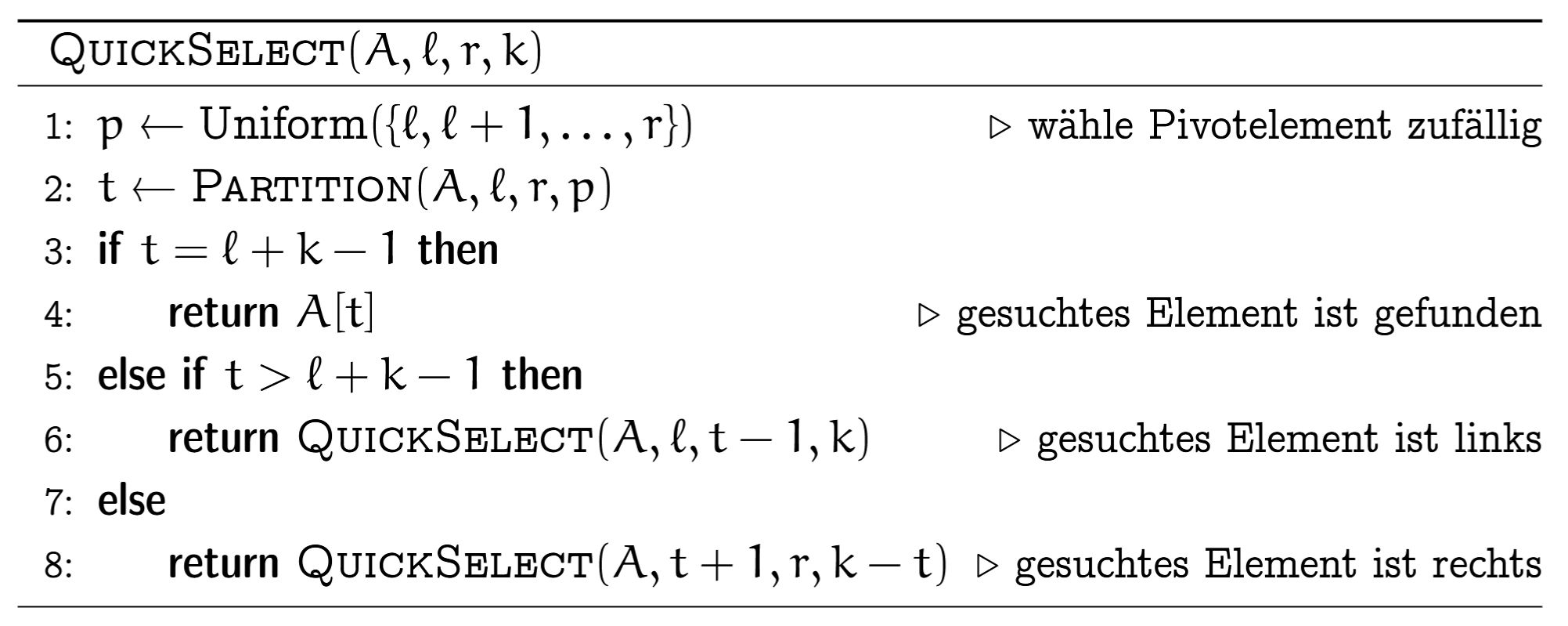
Schneller geht es mit QuickSelect (erwartet \(O(n)\)):
QuickSelect(A, ℓ, r, k):
  p ← Uniform({ℓ, ℓ+1, ..., r})
  t ← Partition(A, ℓ, r, p)
  if t = ℓ + k - 1: return A[t]    # gefunden
  else if t > ℓ + k - 1:
    return QuickSelect(A, ℓ, t-1, k)     # links
  else:
    return QuickSelect(A, t+1, r, k - t) # rechts
Im Gegensatz zu QuickSort rekursiert QuickSelect nur in eine der beiden Hälften (oder gibt direkt zurück, falls Pivot bereits an der gesuchten Position liegt). Das macht den Unterschied zwischen \(O(n \log n)\) und \(O(n)\) erwartet.
Bei einem Aufruf von QuickSelect ist die Anzahl Vergleiche \(T = \sum_{i=1}^{N} (r_i - \ell_i)\), wobei \(N\) die Anzahl Partition-Aufrufe ist.
Schneller geht es mit QuickSelect (erwartet \(O(n)\)):
Im Gegensatz zu QuickSort rekursiert QuickSelect nur in eine der beiden Hälften (oder gibt direkt zurück, falls Pivot bereits an der gesuchten Position liegt). Das macht den Unterschied zwischen \(O(n \log n)\) und \(O(n)\) erwartet.
Bei einem Aufruf von QuickSelect ist die Anzahl Vergleiche \(T = \sum_{i=1}^{N} (r_i - \ell_i)\), wobei \(N\) die Anzahl Partition-Aufrufe ist.
Field-by-field Comparison
Field
Before
After
Text
<b>Selektionsproblem:</b> Bestimme in einer Folge \((A[1], \ldots, A[n])\) paarweise verschiedener Zahlen den {{c1::\(k\)-kleinsten Wert}}.<br><br>Naiver Ansatz: Sortieren + Index, Laufzeit \(O({{c2::n \log n}})\).<br><br>Schneller geht es mit <b>QuickSelect</b> (erwartet \(O({{c3::n}})\)):<pre>QuickSelect(A, ℓ, r, k):
p ← Uniform({ℓ, ℓ+1, ..., r})
t ← Partition(A, ℓ, r, p)
if t = ℓ + k - 1: return A[t] # gefunden
else if t > ℓ + k - 1:
return QuickSelect(A, ℓ, t-1, k) # links
else:
return QuickSelect(A, t+1, r, k - t) # rechts</pre>
<b>Selektionsproblem:</b> Bestimme in einer Folge \((A[1], \ldots, A[n])\) paarweise verschiedener Zahlen den {{c1::\(k\)-kleinsten Wert}}.<br><br>Naiver Ansatz: Sortieren + Index, Laufzeit \(O({{c2::n \log n}})\).<br><br>Schneller geht es mit <b>QuickSelect</b> (erwartet \(O({{c3::n}})\)):<br><br><img src="paste-ec2c4055d88b8fe7537faa99452da2cecee1c287.jpg">
ReachabilityCounting: finaler Union Bound Je Knoten \(v\) gilt \(\Pr[\tilde n_v \leq n_v/20] \leq \tfrac{\delta}{2n}\) und \(\Pr[\tilde n_v \geq 20 n_v] \leq \tfrac{\delta}{2n}\). Über alle \(n\) Knoten und beide Seiten liefert der Union Bound eine Fehlerwahrscheinlichkeit \(\leq {{c1::2n \cdot \tfrac{\delta}{2n} = \delta}}\), also Erfolg mit Wahrscheinlichkeit \(\geq 1-\delta\).
ReachabilityCounting: finaler Union Bound Je Knoten \(v\) gilt \(\Pr[\tilde n_v \leq n_v/20] \leq \tfrac{\delta}{2n}\) und \(\Pr[\tilde n_v \geq 20 n_v] \leq \tfrac{\delta}{2n}\). Über alle \(n\) Knoten und beide Seiten liefert der Union Bound eine Fehlerwahrscheinlichkeit \(\leq {{c1::2n \cdot \tfrac{\delta}{2n} = \delta}}\), also Erfolg mit Wahrscheinlichkeit \(\geq 1-\delta\).
Field-by-field Comparison
Field
Before
After
Text
<b>ReachabilityCounting: finaler Union Bound</b><br>Je Knoten \(v\) gilt \(\Pr[\tilde n_v \leq n_v/20] \leq \tfrac{\delta}{2n}\) und \(\Pr[\tilde n_v \geq 20 n_v] \leq \tfrac{\delta}{2n}\).<br>Über alle \(n\) Knoten und beide Seiten liefert der Union Bound eine Fehlerwahrscheinlichkeit \(\leq {{c1::2n \cdot \tfrac{\delta}{2n} = \delta}}\), also Erfolg mit Wahrscheinlichkeit \(\geq {{c2::1-\delta}}\).
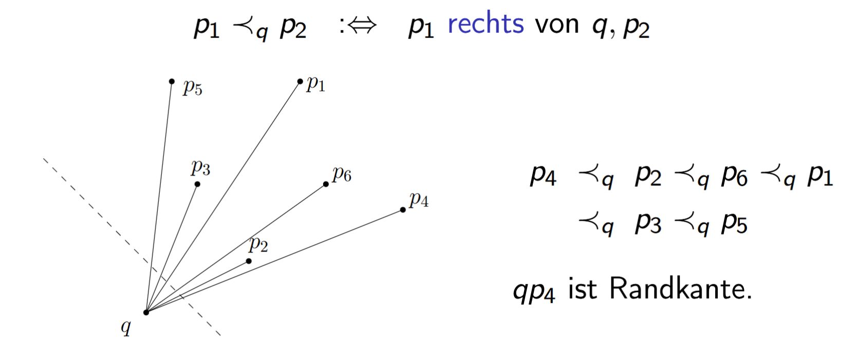
Randkante. Ein Paar \(qr \in P^2\), \(q \neq r\), heisst Randkante von \(P\), falls {{c1::alle Punkte in \(P \setminus \{q, r\}\) links von \(q, r\) liegen}} (d.h. auf der linken Seite der von \(q\) nach \(r\) gerichteten Geraden).
Randkante. Ein Paar \(qr \in P^2\), \(q \neq r\), heisst Randkante von \(P\), falls {{c1::alle Punkte in \(P \setminus \{q, r\}\) links von \(q, r\) liegen}} (d.h. auf der linken Seite der von \(q\) nach \(r\) gerichteten Geraden).
Diese gerichtete Sichtweise legt direkt die Gegen-Uhrzeigersinn-Orientierung der Hülle fest.
Randkante. Ein Paar \(qr \in P^2\), \(q \neq r\), heisst Randkante von \(P\), falls {{c1::alle Punkte in \(P \setminus \{q, r\}\) links von \(q, r\) liegen (d.h. auf der linken Seite der von \(q\) nach \(r\) gerichteten Geraden)}}.
Randkante. Ein Paar \(qr \in P^2\), \(q \neq r\), heisst Randkante von \(P\), falls {{c1::alle Punkte in \(P \setminus \{q, r\}\) links von \(q, r\) liegen (d.h. auf der linken Seite der von \(q\) nach \(r\) gerichteten Geraden)}}.
Diese gerichtete Sichtweise legt direkt die Gegen-Uhrzeigersinn-Orientierung der Hülle fest.
Field-by-field Comparison
Field
Before
After
Text
<b>Randkante.</b><br>Ein Paar \(qr \in P^2\), \(q \neq r\), heisst <b>Randkante</b> von \(P\), falls {{c1::alle Punkte in \(P \setminus \{q, r\}\) links von \(q, r\) liegen}} (d.h. auf der linken Seite der von \(q\) nach \(r\) gerichteten Geraden).
<b>Randkante.</b><br>Ein Paar \(qr \in P^2\), \(q \neq r\), heisst <b>Randkante</b> von \(P\), falls {{c1::alle Punkte in \(P \setminus \{q, r\}\) links von \(q, r\) liegen (d.h. auf der linken Seite der von \(q\) nach \(r\) gerichteten Geraden)}}.
Extra
Diese gerichtete Sichtweise legt direkt die Gegen-Uhrzeigersinn-Orientierung der Hülle fest.
<img src="paste-b9d6d6da2e7f4e631030fd61a74aff893741ae56.jpg"><br><br>Diese gerichtete Sichtweise legt direkt die Gegen-Uhrzeigersinn-Orientierung der Hülle fest.
Idee hinter der Erreichbarkeits-Approximation Wähle \(r_v \leftarrow \mathrm{Uniform}([0,1])\) und setze \(x_v = \min_{u \in R(v)} r_u\).
Dann ist \(x_v\) das Minimum von \(n_v\) Zufallszahlen in \([0,1]\), also grob \(x_v \approx 1/n_v\). Folglich ist \(1/x_v\) eine Schätzung für \(n_v\). Den Fehler reduziert man, indem man über mehrere Läufe den Median bildet.
Field-by-field Comparison
Field
Before
After
Text
<b>Idee hinter der Erreichbarkeits-Approximation</b><br>Wähle \(r_v \leftarrow \mathrm{Uniform}([0,1])\) und setze \(x_v = \min_{u \in R(v)} r_u\).<br><br>Dann ist \(x_v\) das {{c1::Minimum von \(n_v\) Zufallszahlen in \([0,1]\)}}, also grob \(x_v \approx {{c2::1/n_v}}\).<br>Folglich ist {{c3::\(1/x_v\)}} eine Schätzung für \(n_v\).<br>Den Fehler reduziert man, indem man über mehrere Läufe den {{c4::Median}} bildet.
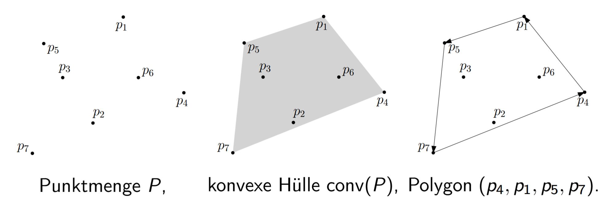
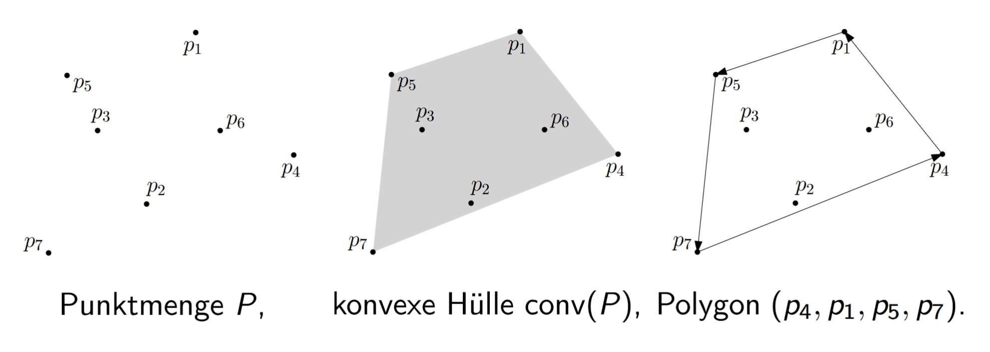
Darstellung der konvexen Hülle (endliches \(P\) in der Ebene). Der Rand von \(\operatorname{conv}(P)\) ist ein Polygon, dessen Ecken Punkte aus \(P\) sind. Die Berechnung von \(\operatorname{conv}(P)\) meint die Bestimmung der Eckenfolge \((q_0, q_1, \ldots, q_{h-1})\), \(h \leq n\), beginnend bei beliebigem \(q_0\) und gegen den Uhrzeigersinn entlang des Polygons.
Dabei ist \(Q := \{q_0, \ldots, q_{h-1}\}\) {{c4::die kleinste Teilmenge von \(P\) mit \(\operatorname{conv}(Q) = \operatorname{conv}(P)\)}}.
Darstellung der konvexen Hülle (endliches \(P\) in der Ebene).
Der Rand von \(\operatorname{conv}(P)\) ist ein Polygon, dessen Ecken Punkte aus \(P\) sind.
Die Berechnung von \(\operatorname{conv}(P)\) meint {{c2::die Bestimmung der Eckenfolge \((q_0, q_1, \ldots, q_{h-1})\), \(h \leq n\), beginnend bei beliebigem \(q_0\) und gegen den Uhrzeigersinn entlang des Polygons}}.
Dabei ist \(Q := \{q_0, \ldots, q_{h-1}\}\) {{c3::die kleinste Teilmenge von \(P\) mit \(\operatorname{conv}(Q) = \operatorname{conv}(P)\)}}.
Field-by-field Comparison
Field
Before
After
Text
<b>Darstellung der konvexen Hülle (endliches \(P\) in der Ebene).</b><br>Der Rand von \(\operatorname{conv}(P)\) ist ein {{c1::Polygon}}, dessen Ecken {{c2::Punkte aus \(P\)}} sind. Die Berechnung von \(\operatorname{conv}(P)\) meint die Bestimmung der Eckenfolge \((q_0, q_1, \ldots, q_{h-1})\), \(h \leq n\), beginnend bei beliebigem \(q_0\) und {{c3::gegen den Uhrzeigersinn}} entlang des Polygons.<br><br>Dabei ist \(Q := \{q_0, \ldots, q_{h-1}\}\) {{c4::die kleinste Teilmenge von \(P\) mit \(\operatorname{conv}(Q) = \operatorname{conv}(P)\)}}.
<b>Darstellung der konvexen Hülle (endliches \(P\) in der Ebene).<br></b><br>Der Rand von \(\operatorname{conv}(P)\) ist {{c1::ein Polygon, dessen Ecken Punkte aus \(P\) sind}}. <br><br>Die Berechnung von \(\operatorname{conv}(P)\) meint {{c2::die Bestimmung der Eckenfolge \((q_0, q_1, \ldots, q_{h-1})\), \(h \leq n\), beginnend bei beliebigem \(q_0\) und gegen den Uhrzeigersinn entlang des Polygons}}.<br><br>Dabei ist \(Q := \{q_0, \ldots, q_{h-1}\}\) {{c3::die kleinste Teilmenge von \(P\) mit \(\operatorname{conv}(Q) = \operatorname{conv}(P)\)}}.
Union-Bound-Fakt Für alle \(x \in [0,1]\) und \(n \in \mathbb{N}\) gilt\[1 - (1-x)^n \leq n x\]Beweisidee: Für unabhängige \(X_1,\ldots,X_n \sim \mathrm{Ber}(x)\) ist \(\Pr[X_1=1 \vee \ldots \vee X_n=1] = 1-(1-x)^n\); die Union Bound liefert andererseits \(\Pr[X_1=1 \vee \ldots \vee X_n=1] \leq \sum_i \Pr[X_i=1] = n x\).
Union-Bound-Fakt Für alle \(x \in [0,1]\) und \(n \in \mathbb{N}\) gilt\[1 - (1-x)^n \leq n x\]Beweisidee: Für unabhängige \(X_1,\ldots,X_n \sim \mathrm{Ber}(x)\) ist \(\Pr[X_1=1 \vee \ldots \vee X_n=1] = 1-(1-x)^n\); die Union Bound liefert andererseits \(\Pr[X_1=1 \vee \ldots \vee X_n=1] \leq \sum_i \Pr[X_i=1] = n x\).
Spezialfall der Booleschen Ungleichung, im Beweis von ReachabilityCounting (Teil 2) verwendet.
Field-by-field Comparison
Field
Before
After
Text
<b>Union-Bound-Fakt</b><br>Für alle \(x \in [0,1]\) und \(n \in \mathbb{N}\) gilt\[{{c1::1 - (1-x)^n \leq n x}}\]Beweisidee: Für unabhängige \(X_1,\ldots,X_n \sim \mathrm{Ber}(x)\) ist \(\Pr[X_1=1 \vee \ldots \vee X_n=1] = {{c2::1-(1-x)^n}}\); die Union Bound liefert andererseits \(\Pr[X_1=1 \vee \ldots \vee X_n=1] \leq \sum_i \Pr[X_i=1] = {{c3::n x}}\).
Extra
Spezialfall der Booleschen Ungleichung, im Beweis von ReachabilityCounting (Teil 2) verwendet.
Nützliche Subroutine Gegeben ein gerichteter Graph \(G\) und Zahlen \(r_v\), berechne für jeden Knoten \(v\) die kleinste erreichbare Zahl \(\min_{u \in R(v)} r_u\).
Naiv \(O(n(n+m))\). Verbesserung auf \(O(n \log n + m)\): Sortiere die Knoten aufsteigend nach \(r_v\) und starte von jedem noch unbesuchten Knoten eine Rückwärts-DFS (entlang eingehender Kanten), die \(\min[\cdot]\) auf den aktuellen Wert setzt.
Subroutine(G, r):
  sortiere V aufsteigend nach r_v: v_1, ..., v_n
  min[v] := ∞ für alle v
  for i = 1, ..., n:
    if min[v_i] = ∞:
      DFSrev(v_i, r_{v_i})
  return min

DFSrev(v, r):
  min[v] := r
  for each eingehender Nachbar u von v:
    if min[u] = ∞:
      DFSrev(u, r)
Bemerkung: Hier ist \(\min\) einfacher zu berechnen als eine Summe \(\sum\).
Field-by-field Comparison
Field
Before
After
Text
<b>Nützliche Subroutine</b><br>Gegeben ein gerichteter Graph \(G\) und Zahlen \(r_v\), berechne für jeden Knoten \(v\) die kleinste erreichbare Zahl \(\min_{u \in R(v)} r_u\).<br><br>Naiv \(O(n(n+m))\). Verbesserung auf {{c1::\(O(n \log n + m)\)}}:<br>Sortiere die Knoten {{c2::aufsteigend nach \(r_v\)}} und starte von jedem noch unbesuchten Knoten eine {{c3::Rückwärts-DFS (entlang eingehender Kanten)}}, die \(\min[\cdot]\) auf den aktuellen Wert setzt.
Extra
<pre>Subroutine(G, r):
sortiere V aufsteigend nach r_v: v_1, ..., v_n
min[v] := ∞ für alle v
for i = 1, ..., n:
if min[v_i] = ∞:
DFSrev(v_i, r_{v_i})
return min
DFSrev(v, r):
min[v] := r
for each eingehender Nachbar u von v:
if min[u] = ∞:
DFSrev(u, r)</pre>Bemerkung: Hier ist \(\min\) einfacher zu berechnen als eine Summe \(\sum\).
Degeneriertheiten sind einfach einzubeziehen (lexikographisch sortieren, Duplikate danach entfernen, Test adaptieren).
Numerisch robuster als JarvisWrap: kann nie in eine unendliche Schleife laufen.
Liefert nebenbei eine Triangulierung der Punkte (lokale Verbesserung dient auch zur Berechnung guter, etwa Delaunay-, Triangulierungen).
Optimal, aber: es gibt auch einen \(O(n \log h)\)-Algorithmus; für Punkte zufällig aus Quadrat/Kreisscheibe sogar erwartet \(O(n)\).
Field-by-field Comparison
Field
Before
After
Text
<b>Anmerkungen zu LocalRepair.</b><br><ul><li>Degeneriertheiten sind einfach einzubeziehen (lexikographisch sortieren, Duplikate danach entfernen, Test adaptieren).</li><li>Numerisch {{c1::robuster als JarvisWrap}}: kann nie in eine unendliche Schleife laufen.</li><li>Liefert nebenbei {{c2::eine Triangulierung der Punkte}} (lokale Verbesserung dient auch zur Berechnung guter, etwa Delaunay-, Triangulierungen).</li><li>Optimal, aber: es gibt auch einen {{c3::\(O(n \log h)\)}}-Algorithmus; für Punkte zufällig aus Quadrat/Kreisscheibe sogar erwartet {{c4::\(O(n)\)}}.</li></ul>
<b>Anmerkungen zu LocalRepair.</b><br><ul><li>Degeneriertheiten sind einfach einzubeziehen (lexikographisch sortieren, Duplikate danach entfernen, Test adaptieren).</li><li>Numerisch {{c1::robuster als JarvisWrap: kann nie in eine unendliche Schleife laufen}}.</li><li>Liefert nebenbei {{c2::eine Triangulierung der Punkte (lokale Verbesserung dient auch zur Berechnung guter, etwa Delaunay-, Triangulierungen)}}.</li><li>Optimal, aber: es gibt auch einen {{c3::\(O(n \log h)\)}}-Algorithmus; für Punkte zufällig aus Quadrat/Kreisscheibe sogar erwartet {{c3::\(O(n)\)}}.</li></ul>
Approximation der Erreichbarkeit (gerichtet) Die Menge der von \(v\) erreichbaren Knoten ist \(R(v) = \{u \in V : u \text{ von } v \text{ erreichbar}\}\), und man schreibt \(n_v = |R(v)|\) für ihre Grösse.
Da exaktes Zählen vermutlich nicht nahe-linear geht, approximiert man \(n_v\): berechne \(\tilde n_v\) mit {{c2::\(\tfrac{n_v}{20} \leq \tilde n_v \leq 20 n_v\)}} (oder sogar \((1-\varepsilon)n_v \leq \tilde n_v \leq (1+\varepsilon)n_v\)).
Field-by-field Comparison
Field
Before
After
Text
<b>Approximation der Erreichbarkeit (gerichtet)</b><br>Die Menge der von \(v\) erreichbaren Knoten ist \(R(v) = \{u \in V : u \text{ von } v \text{ erreichbar}\}\), und man schreibt {{c1::\(n_v = |R(v)|\)}} für ihre Grösse.<br><br>Da exaktes Zählen vermutlich nicht nahe-linear geht, approximiert man \(n_v\): berechne \(\tilde n_v\) mit {{c2::\(\tfrac{n_v}{20} \leq \tilde n_v \leq 20 n_v\)}} (oder sogar \((1-\varepsilon)n_v \leq \tilde n_v \leq (1+\varepsilon)n_v\)).
Vereinfachende Annahme: Allgemeine Lage. Für die ConvexHull-Algorithmen nimmt man an, dass keine 3 Punkte auf einer gemeinsamen Geraden liegen und keine 2 Punkte dieselbe \(x\)-Koordinate haben.
Vereinfachende Annahme: Allgemeine Lage. Für die ConvexHull-Algorithmen nimmt man an, dass keine 3 Punkte auf einer gemeinsamen Geraden liegen und keine 2 Punkte dieselbe \(x\)-Koordinate haben.
Diese Annahme schliesst Kollinearitäten und Mehrdeutigkeiten aus: Degeneriertheiten werden separat behandelt.
Vereinfachende Annahme: Allgemeine Lage. Für die ConvexHull-Algorithmen nimmt man an, dass keine 3 Punkte auf einer gemeinsamen Geraden liegen und keine 2 Punkte dieselbe \(x\)-Koordinate haben.
Vereinfachende Annahme: Allgemeine Lage. Für die ConvexHull-Algorithmen nimmt man an, dass keine 3 Punkte auf einer gemeinsamen Geraden liegen und keine 2 Punkte dieselbe \(x\)-Koordinate haben.
Diese Annahme schliesst Kollinearitäten und Mehrdeutigkeiten aus: Degeneriertheiten werden separat behandelt.
Field-by-field Comparison
Field
Before
After
Text
<b>Vereinfachende Annahme: Allgemeine Lage.</b><br>Für die ConvexHull-Algorithmen nimmt man an, dass {{c1::keine 3 Punkte auf einer gemeinsamen Geraden liegen}} und {{c2::keine 2 Punkte dieselbe \(x\)-Koordinate haben}}.
<b>Vereinfachende Annahme: Allgemeine Lage.</b><br>Für die ConvexHull-Algorithmen nimmt man an, dass {{c1::keine 3 Punkte auf einer gemeinsamen Geraden liegen}} und {{c1::keine 2 Punkte dieselbe \(x\)-Koordinate haben}}.
ReachabilityCounting (Faktor-20-Approximation) Wähle \(\ell = \lceil 2 \log_2(2n/\delta) \rceil\) Läufe. In jedem Lauf \(i\): ziehe \(r_{i,v} \sim \mathrm{Uniform}([0,1])\) und berechne \(x_{i,v} = \min_{u\in R(v)} r_{i,u}\) mit der Subroutine. Setze \(x_v = \mathrm{Median}(x_{1,v}, \ldots, x_{\ell,v})\) und gib \(\tilde n_v = 1/x_v\) zurück.
Laufzeit: \(O((n \log n + m)\log(n/\delta))\).
ReachabilityCounting(G):
  ℓ := ⌈2 log_2(2n/δ)⌉
  for i = 1, ..., ℓ:
    r_{i,v} := Uniform([0,1]) für alle v
    x_{i,v} := min_{u ∈ R(v)} r_{i,u}   # Subroutine, O(n log n + m)
  x_v := Median(x_{1,v}, ..., x_{ℓ,v}) für alle v
  return ñ_v := 1/x_v für alle v
Field-by-field Comparison
Field
Before
After
Text
<b>ReachabilityCounting (Faktor-20-Approximation)</b><br>Wähle {{c1::\(\ell = \lceil 2 \log_2(2n/\delta) \rceil\)}} Läufe. In jedem Lauf \(i\): ziehe \(r_{i,v} \sim \mathrm{Uniform}([0,1])\) und berechne \(x_{i,v} = \min_{u\in R(v)} r_{i,u}\) mit der Subroutine.<br>Setze \(x_v = \mathrm{Median}(x_{1,v}, \ldots, x_{\ell,v})\) und gib {{c2::\(\tilde n_v = 1/x_v\)}} zurück.<br><br>Laufzeit: {{c3::\(O((n \log n + m)\log(n/\delta))\)}}.
Extra
<pre>ReachabilityCounting(G):
ℓ := ⌈2 log_2(2n/δ)⌉
for i = 1, ..., ℓ:
r_{i,v} := Uniform([0,1]) für alle v
x_{i,v} := min_{u ∈ R(v)} r_{i,u} # Subroutine, O(n log n + m)
x_v := Median(x_{1,v}, ..., x_{ℓ,v}) für alle v
return ñ_v := 1/x_v für alle v</pre>
Konsequenz der Invarianten + Nichtdeterminismus. Dank der drei Invarianten gilt: lokal konvex \(\Rightarrow\) Lösungspolygon (kein Selbstschnitt, alle Punkte umschlossen).
Ausserdem ist der Algorithmus zunächst nicht-deterministisch: die lokalen Verbesserungsschritte dürfen in beliebiger Reihenfolge ausgeführt werden.
Field-by-field Comparison
Field
Before
After
Text
<b>Konsequenz der Invarianten + Nichtdeterminismus.</b><br>Dank der drei Invarianten gilt: {{c1::lokal konvex \(\Rightarrow\) Lösungspolygon}} (kein Selbstschnitt, alle Punkte umschlossen).<br><br>Ausserdem ist der Algorithmus zunächst {{c2::nicht-deterministisch}}: die lokalen Verbesserungsschritte dürfen in {{c2::beliebiger Reihenfolge}} ausgeführt werden.
<b>Konsequenz der Invarianten + Nichtdeterminismus.</b><br>Dank der drei Invarianten gilt: {{c1::lokal konvex \(\Rightarrow\) Lösungspolygon (kein Selbstschnitt, alle Punkte umschlossen)}}.<br><br>Ausserdem ist der Algorithmus zunächst {{c2::nicht-deterministisch}}: die lokalen Verbesserungsschritte dürfen in {{c2::beliebiger Reihenfolge}} ausgeführt werden.
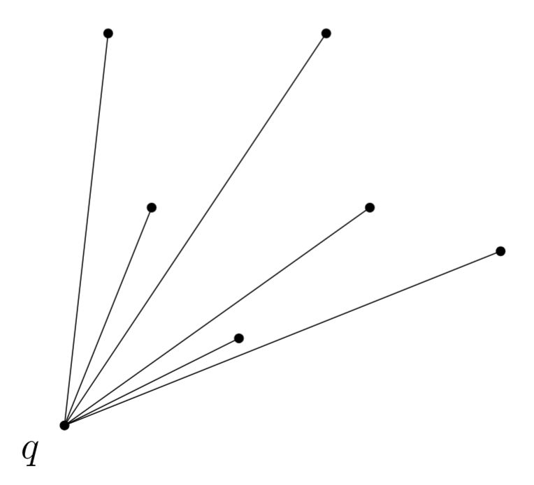
Lemma (Ordnung um eine Hüllen-Ecke). Sei \(q\) eine Ecke der konvexen Hülle von \(P\). Was gilt für die Relation \(\prec_q\) auf \(P \setminus \{q\}\), und was bedeutet ihr Minimum?
Lemma (Ordnung um eine Hüllen-Ecke). Sei \(q\) eine Ecke der konvexen Hülle von \(P\). Was gilt für die Relation \(\prec_q\) auf \(P \setminus \{q\}\), und was bedeutet ihr Minimum?
\(\prec_q\) ist eine totale Ordnung auf \(P \setminus \{q\}\). Für das Minimum \(p_{\min}\) dieser Ordnung gilt: \(q, p_{\min}\) ist eine Randkante.
Damit liefert ein einzelner Min-Durchlauf (wie in FindNext) die nächste Hüllenkante.
Ordnung um eine Hüllen-Ecke. Sei \(q\) eine Ecke der konvexen Hülle von \(P\). Was gilt für die Relation \(\prec_q\) auf \(P \setminus \{q\}\), und was bedeutet ihr Minimum?
Ordnung um eine Hüllen-Ecke. Sei \(q\) eine Ecke der konvexen Hülle von \(P\). Was gilt für die Relation \(\prec_q\) auf \(P \setminus \{q\}\), und was bedeutet ihr Minimum?
\(\prec_q\) ist eine totale Ordnung auf \(P \setminus \{q\}\). Für das Minimum \(p_{\min}\) dieser Ordnung gilt: \(q, p_{\min}\) ist eine Randkante.
Damit liefert ein einzelner Min-Durchlauf (wie in FindNext) die nächste Hüllenkante.
Field-by-field Comparison
Field
Before
After
Front
<b>Lemma (Ordnung um eine Hüllen-Ecke).</b><br>Sei \(q\) eine Ecke der konvexen Hülle von \(P\). Was gilt für die Relation \(\prec_q\) auf \(P \setminus \{q\}\), und was bedeutet ihr Minimum?
<b>Ordnung um eine Hüllen-Ecke.</b><br>Sei \(q\) eine Ecke der konvexen Hülle von \(P\). Was gilt für die Relation \(\prec_q\) auf \(P \setminus \{q\}\), und was bedeutet ihr Minimum?
Back
\(\prec_q\) ist eine <b>totale Ordnung</b> auf \(P \setminus \{q\}\). Für das Minimum \(p_{\min}\) dieser Ordnung gilt: \(q, p_{\min}\) ist eine <b>Randkante</b>.<br><br>Damit liefert ein einzelner Min-Durchlauf (wie in <code>FindNext</code>) die nächste Hüllenkante.
\(\prec_q\) ist eine <b>totale Ordnung</b> auf \(P \setminus \{q\}\). Für das Minimum \(p_{\min}\) dieser Ordnung gilt: \(q, p_{\min}\) ist eine <b>Randkante</b>.<br><br>Damit liefert ein einzelner Min-Durchlauf (wie in <code>FindNext</code>) die nächste Hüllenkante.<br><br><img src="paste-aecdd3cc19feb3435f875933ad9e18b3b9ca0196.jpg">
Distinct Elements / Count-Distinct Welches praktische Problem löst dieselbe Idee wie ReachabilityCounting, und wie?
Man will die Anzahl unterschiedlicher Nutzer bzw. Aufrufe approximieren, ohne alle Aufrufe zu speichern.
Dieselbe Median-von-Minima-Idee (zufällige Werte ziehen, der kleinste beobachtete Wert schätzt die Anzahl distinkter Elemente) löst das Count-Distinct-Problem. Bekannte Varianten: Flajolet-Martin und HyperLogLog.
Field-by-field Comparison
Field
Before
After
Front
<b>Distinct Elements / Count-Distinct</b><br>Welches praktische Problem löst dieselbe Idee wie ReachabilityCounting, und wie?
Back
Man will die Anzahl <b>unterschiedlicher</b> Nutzer bzw. Aufrufe approximieren, ohne alle Aufrufe zu speichern.<br><br>Dieselbe Median-von-Minima-Idee (zufällige Werte ziehen, der kleinste beobachtete Wert schätzt die Anzahl distinkter Elemente) löst das Count-Distinct-Problem. Bekannte Varianten: <b>Flajolet-Martin</b> und <b>HyperLogLog</b>.
JarvisWrap: numerische Probleme. Der Orientierungsausdruck \((r_x - q_x)(p_y - q_y) - (p_x - q_x)(r_y - q_y) > 0\) ist mit Fliesskommazahlen nicht exakt. Kritisch ist dabei oft nicht die absolute Genauigkeit, sondern dass der Algorithmus völlig falsche Ergebnisse liefern oder in eine unendliche Schleife laufen kann (z.B. Vorbeilaufen am Startpunkt, weil dieser doppelt auftritt).
Abhilfe: Programmbibliotheken mit exakten Datentypen (für spezielle Operationen).
Der Orientierungsausdruck \((r_x - q_x)(p_y - q_y) - (p_x - q_x)(r_y - q_y) > 0\) ist mit Fliesskommazahlen nicht exakt.
Kritisch ist dabei oft nicht die absolute Genauigkeit, sondern dass der Algorithmus völlig falsche Ergebnisse liefern oder in eine unendliche Schleife laufen kann (z.B. Vorbeilaufen am Startpunkt, weil dieser doppelt auftritt).
Abhilfe: Programmbibliotheken mit exakten Datentypen (für spezielle Operationen).
Field-by-field Comparison
Field
Before
After
Text
<b>JarvisWrap: numerische Probleme.</b><br>Der Orientierungsausdruck \((r_x - q_x)(p_y - q_y) - (p_x - q_x)(r_y - q_y) > 0\) ist mit Fliesskommazahlen nicht exakt. Kritisch ist dabei oft nicht die absolute Genauigkeit, sondern dass der Algorithmus {{c1::völlig falsche Ergebnisse liefern oder in eine unendliche Schleife laufen}} kann (z.B. {{c2::Vorbeilaufen am Startpunkt}}, weil dieser doppelt auftritt).<br><br>Abhilfe: {{c3::Programmbibliotheken mit exakten Datentypen}} (für spezielle Operationen).
<b>JarvisWrap: numerische Probleme.<br></b><br>Der Orientierungsausdruck \((r_x - q_x)(p_y - q_y) - (p_x - q_x)(r_y - q_y) > 0\) ist mit Fliesskommazahlen nicht exakt. <br><br>Kritisch ist dabei oft nicht die absolute Genauigkeit, sondern dass der Algorithmus {{c1::völlig falsche Ergebnisse liefern oder in eine unendliche Schleife laufen kann (z.B. Vorbeilaufen am Startpunkt, weil dieser doppelt auftritt)}}.<br><br>Abhilfe: {{c2::Programmbibliotheken mit exakten Datentypen (für spezielle Operationen)}}.
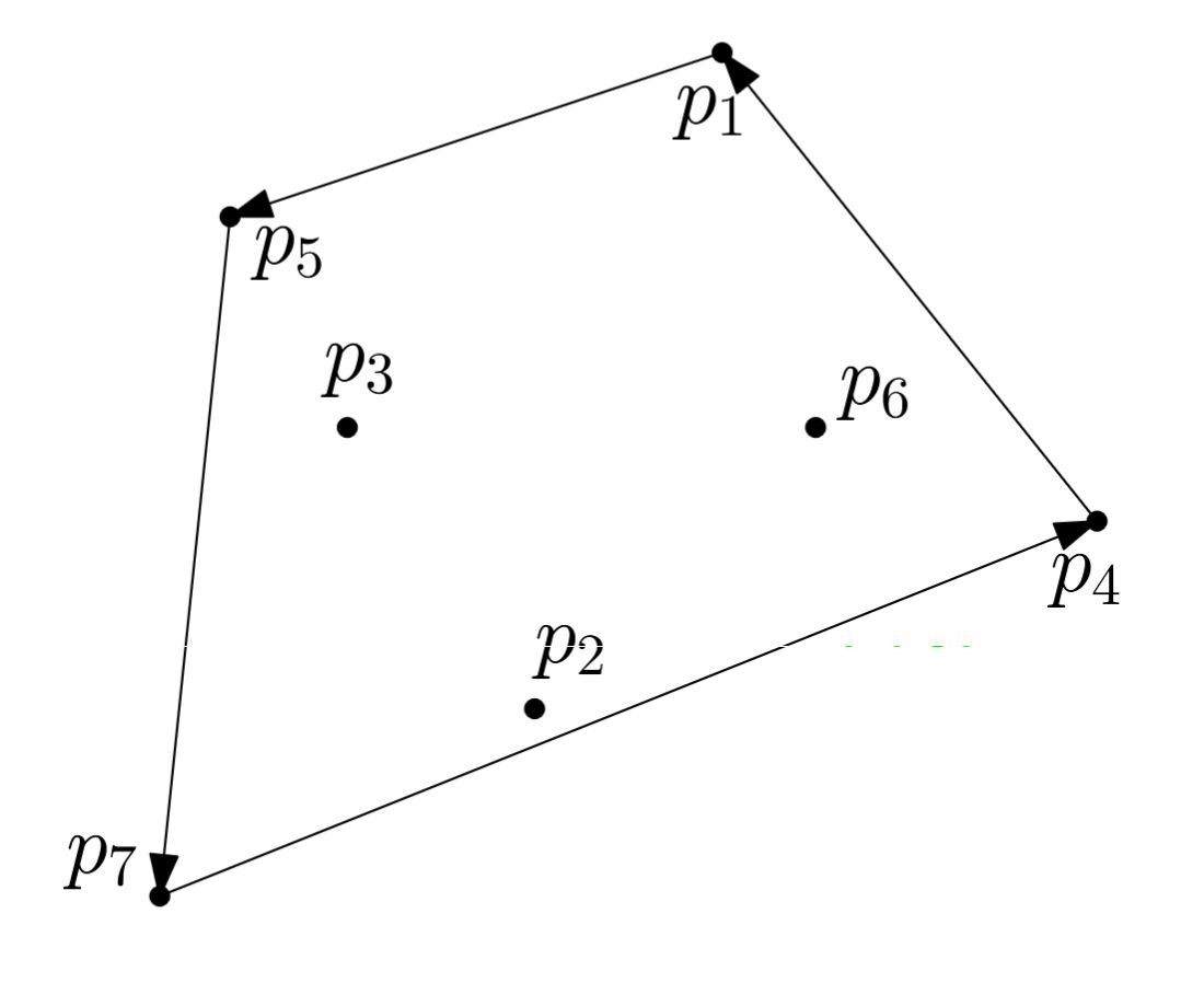
Lemma (Randkanten charakterisieren die Hülle). Wann ist \((q_0, q_1, \ldots, q_{h-1})\) die Eckenfolge des \(\operatorname{conv}(P)\) umschliessenden Polygons gegen den Uhrzeigersinn? (Indizes \(\bmod\, h\))
Lemma (Randkanten charakterisieren die Hülle). Wann ist \((q_0, q_1, \ldots, q_{h-1})\) die Eckenfolge des \(\operatorname{conv}(P)\) umschliessenden Polygons gegen den Uhrzeigersinn? (Indizes \(\bmod\, h\))
Genau dann, wenn alle Paare \((q_{i-1}, q_i)\), \(i = 1, 2, \ldots, h\), Randkanten von \(P\) sind (Indizes \(\bmod\, h\)).
Das übersetzt die globale Eigenschaft "Eckenfolge der Hülle" in lokal prüfbare Randkanten-Bedingungen.
Wann ist \((q_0, q_1, \ldots, q_{h-1})\) die Eckenfolge des \(\operatorname{conv}(P)\) umschliessenden Polygons gegen den Uhrzeigersinn? (Indizes \(\bmod\, h\))
Wann ist \((q_0, q_1, \ldots, q_{h-1})\) die Eckenfolge des \(\operatorname{conv}(P)\) umschliessenden Polygons gegen den Uhrzeigersinn? (Indizes \(\bmod\, h\))
Genau dann, wenn alle Paare \((q_{i-1}, q_i)\), \(i = 1, 2, \ldots, h\), Randkanten von \(P\) sind (Indizes \(\bmod\, h\)).
Das übersetzt die globale Eigenschaft "Eckenfolge der Hülle" in lokal prüfbare Randkanten-Bedingungen.
Field-by-field Comparison
Field
Before
After
Front
<b>Lemma (Randkanten charakterisieren die Hülle).</b><br>Wann ist \((q_0, q_1, \ldots, q_{h-1})\) die Eckenfolge des \(\operatorname{conv}(P)\) umschliessenden Polygons gegen den Uhrzeigersinn? (Indizes \(\bmod\, h\))
Wann ist \((q_0, q_1, \ldots, q_{h-1})\) die Eckenfolge des \(\operatorname{conv}(P)\) umschliessenden Polygons gegen den Uhrzeigersinn? (Indizes \(\bmod\, h\))
Back
<b>Genau dann, wenn</b> alle Paare \((q_{i-1}, q_i)\), \(i = 1, 2, \ldots, h\), <b>Randkanten von \(P\)</b> sind (Indizes \(\bmod\, h\)).<br><br>Das übersetzt die globale Eigenschaft "Eckenfolge der Hülle" in lokal prüfbare Randkanten-Bedingungen.
<b>Genau dann, wenn</b> alle Paare \((q_{i-1}, q_i)\), \(i = 1, 2, \ldots, h\), <b>Randkanten von \(P\)</b> sind (Indizes \(\bmod\, h\)).<br><br><img src="paste-12efe5806bf069f8d56fa92f61f53fa07d83a93d.jpg"><br><br>Das übersetzt die globale Eigenschaft "Eckenfolge der Hülle" in lokal prüfbare Randkanten-Bedingungen.
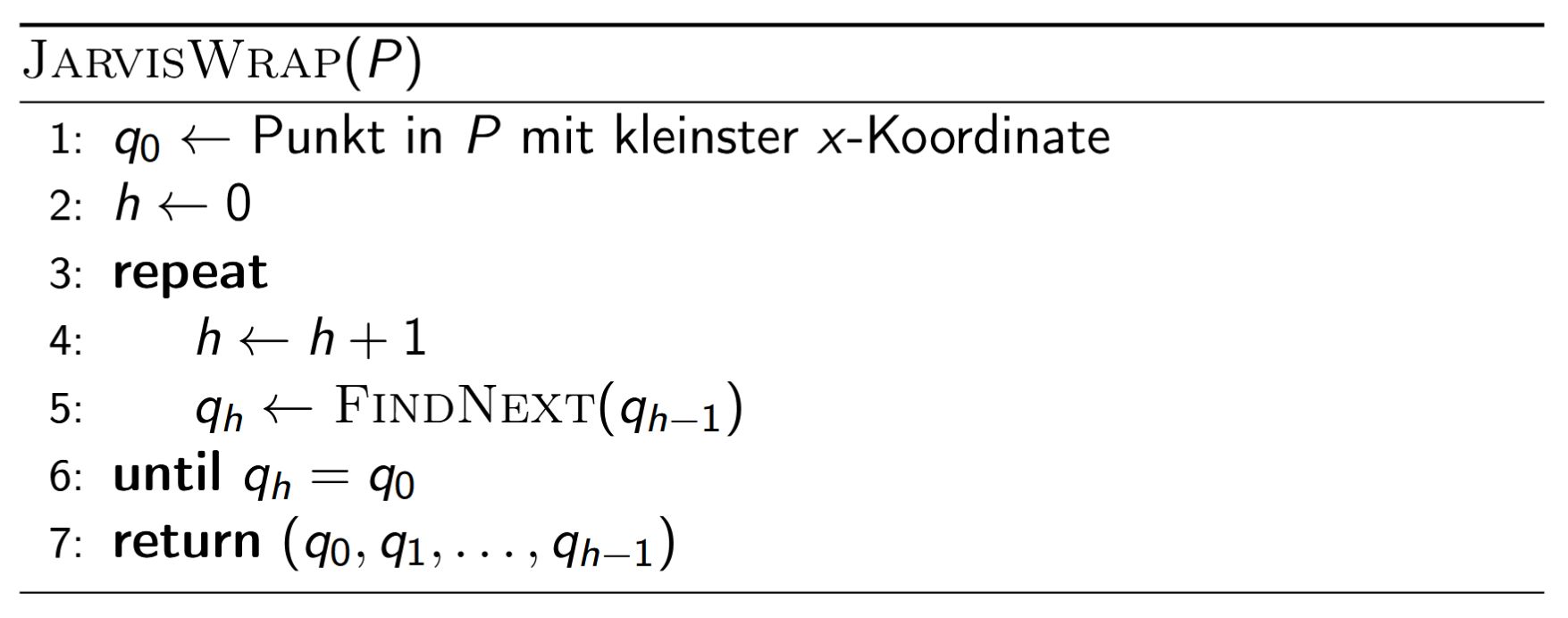
Jarvis Wrap (Einwickeln). Startend bei \(q_0\) (kleinste \(x\)-Koordinate) hängt man wiederholt {{c1::\(q_h \leftarrow \texttt{FindNext}(q_{h-1})\)}} an, bis \(q_h = q_0\) (die Hülle ist geschlossen):
JarvisWrap(P):
  q₀ ← Punkt in P mit kleinster x-Koordinate
  h ← 0
  repeat:
    h ← h + 1
    q_h ← FindNext(q_{h-1})
  until q_h = q₀
  return (q₀, q₁, ..., q_{h-1})
Jarvis Wrap (Einwickeln). Startend bei \(q_0\) (kleinste \(x\)-Koordinate) hängt man wiederholt {{c1::\(q_h \leftarrow \texttt{FindNext}(q_{h-1})\)}} an, bis \(q_h = q_0\) (die Hülle ist geschlossen):
Jarvis Wrap (Einwickeln). Startend bei \(q_0\) (kleinste \(x\)-Koordinate) hängt man wiederholt {{c1::\(q_h \leftarrow \texttt{FindNext}(q_{h-1})\)}} an, bis \(q_h = q_0\) (die Hülle ist geschlossen):
Field-by-field Comparison
Field
Before
After
Text
<b>Jarvis Wrap (Einwickeln).</b><br>Startend bei \(q_0\) (kleinste \(x\)-Koordinate) hängt man wiederholt {{c1::\(q_h \leftarrow \texttt{FindNext}(q_{h-1})\)}} an, bis {{c2::\(q_h = q_0\)}} (die Hülle ist geschlossen):<pre>JarvisWrap(P):
q₀ ← Punkt in P mit kleinster x-Koordinate
h ← 0
repeat:
h ← h + 1
q_h ← FindNext(q_{h-1})
until q_h = q₀
return (q₀, q₁, ..., q_{h-1})</pre>
<b>Jarvis Wrap (Einwickeln).</b><br>Startend bei \(q_0\) (kleinste \(x\)-Koordinate) hängt man wiederholt {{c1::\(q_h \leftarrow \texttt{FindNext}(q_{h-1})\)}} an, bis {{c1::\(q_h = q_0\) (die Hülle ist geschlossen)}}:
In welcher Zeit berechnet JarvisWrap die konvexe Hülle von \(n\) Punkten in allgemeiner Lage in \(\mathbb{R}^2\)?
In Zeit \(O(nh)\), wobei \(h\) die Anzahl der Ecken der konvexen Hülle von \(P\) ist.
Jeder der \(h\) FindNext-Aufrufe kostet \(O(n)\) (output-sensitiv).
Field-by-field Comparison
Field
Before
After
Front
<b>Satz: Laufzeit von JarvisWrap.</b><br>In welcher Zeit berechnet JarvisWrap die konvexe Hülle von \(n\) Punkten in allgemeiner Lage in \(\mathbb{R}^2\)?
In welcher Zeit berechnet JarvisWrap die konvexe Hülle von \(n\) Punkten in allgemeiner Lage in \(\mathbb{R}^2\)?
LocalRepair: Laufzeitanalyse. Start mit \(2(n-1)\) Ecken, Ende mit \(h\) Ecken, also genau \(2(n-1) - h = O(n)\) erfolgreiche (entfernende) Tests. Pro Punkt \(p_i\) gibt es zudem zwei erfolglose Tests (einmal unten, einmal oben).
Nach dem anfänglichen Sortieren in \(O(n \log n)\) ist die eigentliche Reparatur also \(O(n)\).
Field-by-field Comparison
Field
Before
After
Text
<b>LocalRepair: Laufzeitanalyse.</b><br>Start mit \(2(n-1)\) Ecken, Ende mit \(h\) Ecken, also genau {{c1::\(2(n-1) - h = O(n)\)}} erfolgreiche (entfernende) Tests. Pro Punkt \(p_i\) gibt es zudem {{c2::zwei erfolglose Tests}} (einmal unten, einmal oben).<br><br>Nach dem anfänglichen Sortieren in \(O(n \log n)\) ist die eigentliche Reparatur also {{c3::\(O(n)\)}}.
<b>LocalRepair: Laufzeitanalyse.</b><br>Start mit \(2(n-1)\) Ecken, Ende mit \(h\) Ecken, also genau {{c1::\(2(n-1) - h = O(n)\)}} erfolgreiche (entfernende) Tests. Pro Punkt \(p_i\) gibt es zudem {{c2::zwei erfolglose Tests (einmal unten, einmal oben)}}.<br><br>Nach dem anfänglichen Sortieren in \(O(n \log n)\) ist die eigentliche Reparatur also {{c1::\(O(n)\)}}.
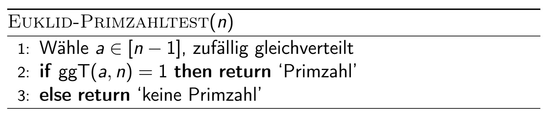
Designziel für Primzahltests: Laufzeit polynomiell in \(\log n\) (Darstellungsgrösse). Naives Trial-Division bis \(\sqrt{n}\) ist zu langsam für \(n \approx 2^{1000}\).
Der \(\mathrm{ggT}\) zweier Zahlen \(m, n\) lässt sich mit dem Euklid-Algorithmus in \(O((\log nm)^3)\) berechnen. Damit:
Euklid-Primzahltest(n):
  wähle a ∈ [n-1] zufällig gleichverteilt
  if ggT(a, n) = 1: return 'Primzahl'
  else: return 'keine Primzahl'
Korrektheit:
Falls \(n\) prim: Ausgabe immer korrekt (alle \(a \in [n-1]\) sind teilerfremd zu \(n\)).
Falls \(n\) nicht prim: Falsche Ausgabe 'Primzahl' mit Wahrscheinlichkeit {{c3::\(\frac{|\mathbb{Z}_n^*|}{n-1}\)}}.
Trivialerweise gilt: \(\mathrm{ggT}(a, n) > 1\) für ein \(a \in [n-1]\) \(\Rightarrow\) \(n\) nicht prim. Der Test sucht also einen kleinen gemeinsamen Faktor mit zufälligem \(a\).
Problem: für \(n = p^2\) ist die Fehlerrate \(\approx 1 - 1/\sqrt{n}\), also fast \(1\). Der Test ist deshalb in der Praxis nutzlos.
Designziel für Primzahltests: Laufzeit polynomiell in \(\log n\) (Darstellungsgrösse). Naives Trial-Division bis \(\sqrt{n}\) ist zu langsam für \(n \approx 2^{1000}\).
Der \(\mathrm{ggT}\) zweier Zahlen \(m, n\) lässt sich mit dem Euklid-Algorithmus in \(O((\log nm)^3)\) berechnen. Damit:
Korrektheit:
Falls \(n\) prim: Ausgabe immer korrekt (alle \(a \in [n-1]\) sind teilerfremd zu \(n\)).
Falls \(n\) nicht prim: Falsche Ausgabe 'Primzahl' mit Wahrscheinlichkeit {{c3::\(\frac{|\mathbb{Z}_n^*|}{n-1}\)}}.
Trivialerweise gilt: \(\mathrm{ggT}(a, n) > 1\) für ein \(a \in [n-1]\) \(\Rightarrow\) \(n\) nicht prim. Der Test sucht also einen kleinen gemeinsamen Faktor mit zufälligem \(a\).
Problem: für \(n = p^2\) ist die Fehlerrate \(\approx 1 - 1/\sqrt{n}\), also fast \(1\). Der Test ist deshalb in der Praxis nutzlos.
Field-by-field Comparison
Field
Before
After
Text
Designziel für Primzahltests: Laufzeit polynomiell in \(\log n\) (Darstellungsgrösse). Naives Trial-Division bis \(\sqrt{n}\) ist zu langsam für \(n \approx 2^{1000}\).<br><br>Der \(\mathrm{ggT}\) zweier Zahlen \(m, n\) lässt sich mit dem Euklid-Algorithmus in \(O({{c1::(\log nm)^3}})\) berechnen. Damit:<pre>Euklid-Primzahltest(n):
wähle a ∈ [n-1] zufällig gleichverteilt
if ggT(a, n) = 1: return 'Primzahl'
else: return 'keine Primzahl'</pre>Korrektheit:<ul><li>Falls \(n\) prim: {{c2::Ausgabe immer korrekt (alle \(a \in [n-1]\) sind teilerfremd zu \(n\))}}.</li><li>Falls \(n\) nicht prim: Falsche Ausgabe 'Primzahl' mit Wahrscheinlichkeit {{c3::\(\frac{|\mathbb{Z}_n^*|}{n-1}\)}}.</li></ul>
Designziel für Primzahltests: Laufzeit polynomiell in \(\log n\) (Darstellungsgrösse). Naives Trial-Division bis \(\sqrt{n}\) ist zu langsam für \(n \approx 2^{1000}\).<br><br>Der \(\mathrm{ggT}\) zweier Zahlen \(m, n\) lässt sich mit dem Euklid-Algorithmus in \(O({{c1::(\log nm)^3}})\) berechnen. Damit:<br><br><img src="paste-6f9413d03db5f86f9dbc5fa17bdff6435967627d.jpg"><br><br>Korrektheit:<ul><li>Falls \(n\) prim: {{c2::Ausgabe immer korrekt (alle \(a \in [n-1]\) sind teilerfremd zu \(n\))}}.</li><li>Falls \(n\) nicht prim: Falsche Ausgabe 'Primzahl' mit Wahrscheinlichkeit {{c3::\(\frac{|\mathbb{Z}_n^*|}{n-1}\)}}.</li></ul>
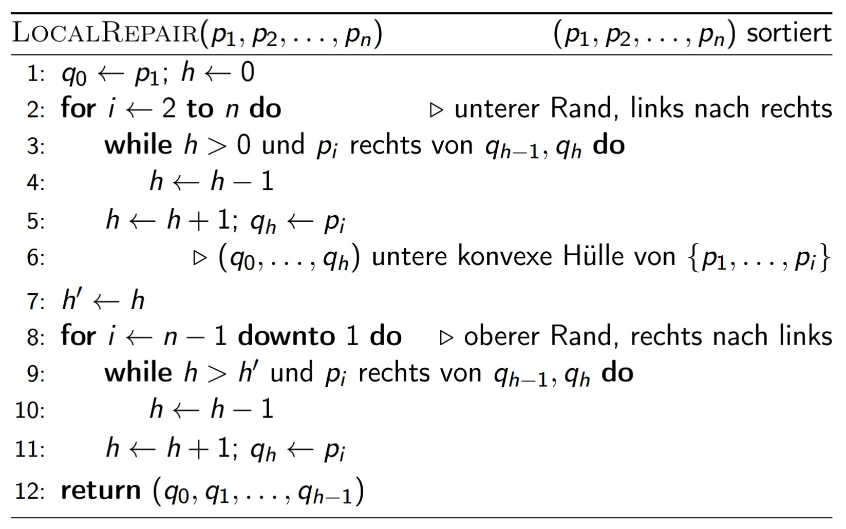
LocalRepair (Eingabe \((p_1, \ldots, p_n)\) nach \(x\)-Koordinate sortiert). Zwei Sweeps: erst unterer Rand, links nach rechts, dann oberer Rand, rechts nach links; jeweils wird \(q_i\) per Pop entfernt, solange \(p_i\) rechts von \(q_{h-1}, q_h\) liegt:
LocalRepair(p₁, ..., p_n):   # sortiert
  q₀ ← p₁; h ← 0
  for i ← 2 to n:              # unterer Rand, links→rechts
    while h > 0 and p_i rechts von q_{h-1}, q_h:
      h ← h - 1
    h ← h + 1; q_h ← p_i
  h' ← h
  for i ← n-1 downto 1:        # oberer Rand, rechts→links
    while h > h' and p_i rechts von q_{h-1}, q_h:
      h ← h - 1
    h ← h + 1; q_h ← p_i
  return (q₀, q₁, ..., q_{h-1})
Nach der ersten Schleife ist \((q_0, \ldots, q_h)\) die untere konvexe Hülle von \(\{p_1, \ldots, p_n\}\); die Schranke \(h > h'\) verhindert, dass der obere Sweep in den unteren Rand hineinläuft.
LocalRepair (Eingabe \((p_1, \ldots, p_n)\) nach \(x\)-Koordinate sortiert). Zwei Sweeps: erst unterer Rand, links nach rechts, dann oberer Rand, rechts nach links; jeweils wird \(q_i\) per Pop entfernt, solange \(p_i\) rechts von \(q_{h-1}, q_h\) liegt:
LocalRepair (Eingabe \((p_1, \ldots, p_n)\) nach \(x\)-Koordinate sortiert). Zwei Sweeps: erst unterer Rand, links nach rechts, dann oberer Rand, rechts nach links; jeweils wird \(q_i\) per Pop entfernt, solange \(p_i\) rechts von \(q_{h-1}, q_h\) liegt:
Nach der ersten Schleife ist \((q_0, \ldots, q_h)\) die untere konvexe Hülle von \(\{p_1, \ldots, p_n\}\); die Schranke \(h > h'\) verhindert, dass der obere Sweep in den unteren Rand hineinläuft.
Field-by-field Comparison
Field
Before
After
Text
<b>LocalRepair</b> (Eingabe \((p_1, \ldots, p_n)\) nach \(x\)-Koordinate sortiert).<br>Zwei Sweeps: erst {{c1::unterer Rand, links nach rechts}}, dann {{c2::oberer Rand, rechts nach links}}; jeweils wird \(q_i\) per Pop entfernt, solange \(p_i\) rechts von \(q_{h-1}, q_h\) liegt:<pre>LocalRepair(p₁, ..., p_n): # sortiert
q₀ ← p₁; h ← 0
for i ← 2 to n: # unterer Rand, links→rechts
while h > 0 and p_i rechts von q_{h-1}, q_h:
h ← h - 1
h ← h + 1; q_h ← p_i
h' ← h
for i ← n-1 downto 1: # oberer Rand, rechts→links
while h > h' and p_i rechts von q_{h-1}, q_h:
h ← h - 1
h ← h + 1; q_h ← p_i
return (q₀, q₁, ..., q_{h-1})</pre>
<b>LocalRepair</b> (Eingabe \((p_1, \ldots, p_n)\) nach \(x\)-Koordinate sortiert).<br>Zwei Sweeps: erst {{c1::unterer Rand, links nach rechts}}, dann {{c1::oberer Rand, rechts nach links}}; jeweils wird \(q_i\) per Pop entfernt, solange \(p_i\) rechts von \(q_{h-1}, q_h\) liegt:<br><br><img src="paste-42be178c67df8469988fbf9c0a012b8a4d83abde.jpg">
JarvisWrap: Umgang mit Degeneriertheiten (Kollinearitäten, gleiche \(x\)-Koordinaten, Duplikate).
Startpunkt \(q_0\): nimm den Punkt mit lexikographisch kleinster Koordinate (unter kleinster \(x\)-Koordinate den mit kleinster \(y\)-Koordinate).
Test "\(p\) rechts von \(q, q_{\text{next} }\)" ersetzen durch: rechts von \(q, q_{\text{next} }\) {{c2::oder (\(p\) auf der Geraden durch \(q, q_{\text{next} }\) und \(|qp| > |q q_{\text{next} }|\))}}.
Punkte sind i.d.R. nicht einmal verschieden (z.B. in einem Feld gegeben).
Software ohne Berücksichtigung dieser Fälle hat geringen praktischen Nutzen.
JarvisWrap: Umgang mit Degeneriertheiten (Kollinearitäten, gleiche \(x\)-Koordinaten, Duplikate).
Startpunkt \(q_0\): nimm den Punkt mit lexikographisch kleinster Koordinate (unter kleinster \(x\)-Koordinate den mit kleinster \(y\)-Koordinate).
Test "\(p\) rechts von \(q, q_{\text{next} }\)" ersetzen durch: {{c2::rechts von \(q, q_{\text{next} }\) oder (\(p\) auf der Geraden durch \(q, q_{\text{next} }\) und \(|qp| > |q q_{\text{next} }|\))}}.
Punkte sind i.d.R. nicht einmal verschieden (z.B. in einem Feld gegeben).
Software ohne Berücksichtigung dieser Fälle hat geringen praktischen Nutzen.
Field-by-field Comparison
Field
Before
After
Text
<b>JarvisWrap: Umgang mit Degeneriertheiten</b> (Kollinearitäten, gleiche \(x\)-Koordinaten, Duplikate).<br><ul><li>Startpunkt \(q_0\): nimm den Punkt mit {{c1::lexikographisch kleinster Koordinate}} (unter kleinster \(x\)-Koordinate den mit kleinster \(y\)-Koordinate).</li><li>Test "\(p\) rechts von \(q, q_{\text{next} }\)" ersetzen durch: rechts von \(q, q_{\text{next} }\) {{c2::oder (\(p\) auf der Geraden durch \(q, q_{\text{next} }\) und \(|qp| > |q q_{\text{next} }|\))}}.</li><li>Punkte sind i.d.R. {{c3::nicht einmal verschieden}} (z.B. in einem Feld gegeben).</li></ul>
<b>JarvisWrap: Umgang mit Degeneriertheiten</b> (Kollinearitäten, gleiche \(x\)-Koordinaten, Duplikate).<br><ul><li>Startpunkt \(q_0\): nimm den Punkt mit {{c1::lexikographisch kleinster Koordinate (unter kleinster \(x\)-Koordinate den mit kleinster \(y\)-Koordinate)}}.</li><li>Test "\(p\) rechts von \(q, q_{\text{next} }\)" ersetzen durch: {{c2::rechts von \(q, q_{\text{next} }\) oder (\(p\) auf der Geraden durch \(q, q_{\text{next} }\) und \(|qp| > |q q_{\text{next} }|\))}}.</li><li>Punkte sind i.d.R. {{c3::nicht einmal verschieden (z.B. in einem Feld gegeben)}}.</li></ul>
Der Algorithmus funktioniert auch für die kleinste umschliessende Kugel (oder Ellipse) in allen Dimensionen, mit anderen Konstanten statt der \(11\). Bei fixer Dimension bleibt die Laufzeit \(O(n \log n)\).
Es gibt auch einfache randomisierte und sogar deterministische Linearzeit-Algorithmen (in jeder fixen Dimension).
Idee von [Clarkson '95].
Field-by-field Comparison
Field
Before
After
Text
<b>Anmerkungen zum Clarkson-Algorithmus.</b><br><ul><li>Der Algorithmus funktioniert auch für die kleinste umschliessende Kugel (oder Ellipse) in {{c1::allen Dimensionen}}, mit anderen Konstanten statt der \(11\). Bei {{c2::fixer Dimension}} bleibt die Laufzeit \(O(n \log n)\).</li><li>Es gibt auch einfache randomisierte und sogar deterministische {{c3::Linearzeit}}-Algorithmen (in jeder fixen Dimension).</li></ul>
<b>Anmerkungen zum Clarkson-Algorithmus.</b><br><ul><li>Der Algorithmus funktioniert auch für die kleinste umschliessende Kugel (oder Ellipse) in {{c1::allen Dimensionen}}, mit anderen Konstanten statt der \(11\). Bei {{c1::fixer Dimension}} bleibt die Laufzeit \(O(n \log n)\).</li><li>Es gibt auch einfache randomisierte und sogar deterministische {{c2::Linearzeit}}-Algorithmen (in jeder fixen Dimension).</li></ul>
Zählen erreichbarer Knoten (gerichtet): Laufzeit Für einen einzelnen Startknoten \(s\) bestimmt ein DFS/BFS die Anzahl erreichbarer Knoten in Zeit \(O(n + m)\). Für alle Knoten ergibt das \(O(n(n + m))\).
Geht es schneller? Vermutlich nicht: Ein \(O(n^{0.99}(n+m))\)-Algorithmus würde \(k\)-SAT in \(O(1.999^n)\) lösen und damit der starken Exponentialzeithypothese (SETH) widersprechen.
Field-by-field Comparison
Field
Before
After
Text
<b>Zählen erreichbarer Knoten (gerichtet): Laufzeit</b><br>Für einen <b>einzelnen</b> Startknoten \(s\) bestimmt ein DFS/BFS die Anzahl erreichbarer Knoten in Zeit \({{c1::O(n + m)}}\).<br>Für <b>alle</b> Knoten ergibt das \({{c2::O(n(n + m))}}\).<br><br>Geht es schneller? {{c3::Vermutlich nicht}}: Ein \(O(n^{0.99}(n+m))\)-Algorithmus würde \(k\)-SAT in \(O(1.999^n)\) lösen und damit der {{c4::starken Exponentialzeithypothese (SETH)}} widersprechen.
Zählen erreichbarer Knoten (ungerichtet) Gegeben ein ungerichteter Graph \(G\), bestimme für jeden Knoten \(v\) die Anzahl erreichbarer Knoten.
Idee: Berechne mit DFS die Zusammenhangskomponenten; die Antwort für \(v\) ist dann die Grösse der Komponente von \(v\). Laufzeit: \(O(n + m)\).
Konkret markiert ConnectedComponents jede Komponente mit einer eigenen Zahl, danach zählt man die Komponentengrössen \(\mathrm{cnt}[c]\) und setzt \(\mathrm{res}[v] = \mathrm{cnt}[\mathrm{comp}[v]]\).
Field-by-field Comparison
Field
Before
After
Text
<b>Zählen erreichbarer Knoten (ungerichtet)</b><br>Gegeben ein ungerichteter Graph \(G\), bestimme für jeden Knoten \(v\) die Anzahl erreichbarer Knoten.<br><br>Idee: Berechne mit DFS die {{c1::Zusammenhangskomponenten}}; die Antwort für \(v\) ist dann die {{c2::Grösse der Komponente von \(v\)}}.<br>Laufzeit: \({{c3::O(n + m)}}\).
Extra
Konkret markiert <code>ConnectedComponents</code> jede Komponente mit einer eigenen Zahl, danach zählt man die Komponentengrössen \(\mathrm{cnt}[c]\) und setzt \(\mathrm{res}[v] = \mathrm{cnt}[\mathrm{comp}[v]]\).
ConvexHull-Problem. Gegeben eine endliche Punktmenge {{c1::\(P \subseteq \mathbb{R}^2\)}}, bestimme die konvexe Hülle von \(P\).
In der Praxis heisst das konkret: bestimme {{c3::die Ecken des \(\operatorname{conv}(P)\) umrandenden Polygons, in der Reihenfolge gegen den Uhrzeigersinn}}.
ConvexHull-Problem. Gegeben eine endliche Punktmenge {{c1::\(P \subseteq \mathbb{R}^2\)}}, bestimme die konvexe Hülle von \(P\).
In der Praxis heisst das konkret: bestimme {{c3::die Ecken des \(\operatorname{conv}(P)\) umrandenden Polygons, in der Reihenfolge gegen den Uhrzeigersinn}}.
ConvexHull-Problem. Gegeben {{c1::eine endliche Punktmenge \(P \subseteq \mathbb{R}^2\)}}, bestimme die konvexe Hülle von \(P\).
In der Praxis heisst das konkret: bestimme {{c2::die Ecken des \(\operatorname{conv}(P)\) umrandenden Polygons, in der Reihenfolge gegen den Uhrzeigersinn}}.
ConvexHull-Problem. Gegeben {{c1::eine endliche Punktmenge \(P \subseteq \mathbb{R}^2\)}}, bestimme die konvexe Hülle von \(P\).
In der Praxis heisst das konkret: bestimme {{c2::die Ecken des \(\operatorname{conv}(P)\) umrandenden Polygons, in der Reihenfolge gegen den Uhrzeigersinn}}.
Field-by-field Comparison
Field
Before
After
Text
<b>ConvexHull-Problem.</b><br>Gegeben eine endliche Punktmenge {{c1::\(P \subseteq \mathbb{R}^2\)}}, bestimme {{c2::die konvexe Hülle von \(P\)}}.<br><br>In der Praxis heisst das konkret: bestimme {{c3::die Ecken des \(\operatorname{conv}(P)\) umrandenden Polygons, in der Reihenfolge gegen den Uhrzeigersinn}}.
<b>ConvexHull-Problem.</b><br>Gegeben {{c1::eine endliche Punktmenge \(P \subseteq \mathbb{R}^2\)}}, bestimme die konvexe Hülle von \(P\).<br><br>In der Praxis heisst das konkret: bestimme {{c2::die Ecken des \(\operatorname{conv}(P)\) umrandenden Polygons, in der Reihenfolge gegen den Uhrzeigersinn}}.
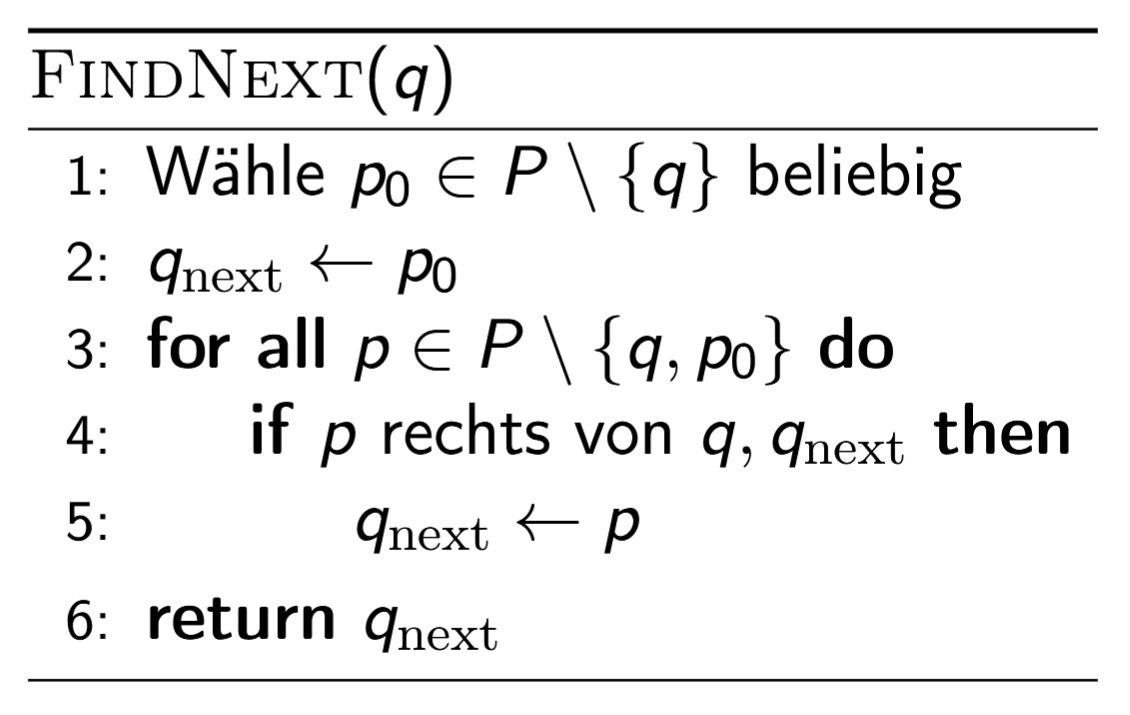
Startpunkt und FindNext. Wähle \(q_0 :=\) Punkt mit kleinster \(x\)-Koordinate in \(P\); dieser ist sicher eine Ecke der konvexen Hülle.
FindNext(q) findet den nächsten Hüllenpunkt, indem es startend mit beliebigem \(p_0\) jeden Punkt durchgeht und \(q_{\text{next} }\) ersetzt, sobald {{c3::\(p\) rechts von \(q, q_{\text{next} }\) liegt}}:
FindNext(q):
  wähle p₀ ∈ P \ {q} beliebig
  q_next ← p₀
  for all p ∈ P \ {q, p₀}:
    if p rechts von q, q_next:
      q_next ← p
  return q_next
Startpunkt und FindNext. Wähle \(q_0 :=\) Punkt mit kleinster \(x\)-Koordinate in \(P\); dieser ist sicher eine Ecke der konvexen Hülle.
FindNext(q) findet den nächsten Hüllenpunkt, indem es startend mit beliebigem \(p_0\) jeden Punkt durchgeht und \(q_{\text{next} }\) ersetzt, sobald {{c3::\(p\) rechts von \(q, q_{\text{next} }\) liegt}}:
Field-by-field Comparison
Field
Before
After
Text
<b>Startpunkt und FindNext.</b><br>Wähle \(q_0 :=\) {{c1::Punkt mit kleinster \(x\)-Koordinate in \(P\)}}; dieser ist sicher {{c2::eine Ecke der konvexen Hülle}}.<br><br><code>FindNext(q)</code> findet den nächsten Hüllenpunkt, indem es startend mit beliebigem \(p_0\) jeden Punkt durchgeht und \(q_{\text{next} }\) ersetzt, sobald {{c3::\(p\) rechts von \(q, q_{\text{next} }\) liegt}}:<pre>FindNext(q):
wähle p₀ ∈ P \ {q} beliebig
q_next ← p₀
for all p ∈ P \ {q, p₀}:
if p rechts von q, q_next:
q_next ← p
return q_next</pre>
<b>Startpunkt und FindNext.</b><br>Wähle \(q_0 :=\) {{c1::Punkt mit kleinster \(x\)-Koordinate in \(P\)}}; dieser ist sicher {{c2::eine Ecke der konvexen Hülle}}.<br><br><code>FindNext(q)</code> findet den nächsten Hüllenpunkt, indem es startend mit beliebigem \(p_0\) jeden Punkt durchgeht und \(q_{\text{next} }\) ersetzt, sobald {{c3::\(p\) rechts von \(q, q_{\text{next} }\) liegt}}:<br><br><img src="paste-8d336e2090420fa0d8fafedb9c6d421ac7dbb985.jpg">
Konvexe Hülle \(\operatorname{conv}(S)\). Die konvexe Hülle einer Menge \(S \subseteq \mathbb{R}^d\) ist der Schnitt aller konvexen Mengen, die \(S\) enthalten:\[\operatorname{conv}(S) := {{c1::\bigcap_{S \subseteq C \subseteq \mathbb{R}^d,\ C \text{ konvex} } C}}.\]Äquivalent: (i) der Schnitt aller Halbebenen, die \(S\) enthalten, (ii) die kleinste konvexe Menge, die \(S\) enthält.
Konvexe Hülle \(\operatorname{conv}(S)\). Die konvexe Hülle einer Menge \(S \subseteq \mathbb{R}^d\) ist der Schnitt aller konvexen Mengen, die \(S\) enthalten:\[\operatorname{conv}(S) := {{c1::\bigcap_{S \subseteq C \subseteq \mathbb{R}^d,\ C \text{ konvex} } C}}.\]Äquivalent: (i) der Schnitt aller Halbebenen, die \(S\) enthalten, (ii) die kleinste konvexe Menge, die \(S\) enthält.
Konvexe Hülle \(\operatorname{conv}(S)\). Die konvexe Hülle einer Menge \(S \subseteq \mathbb{R}^d\) ist der Schnitt aller konvexen Mengen, die \(S\) enthalten:\[\operatorname{conv}(S) := {{c1::\bigcap_{S \subseteq C \subseteq \mathbb{R}^d,\ C \text{ konvex} } C}}.\]Äquivalent:
Konvexe Hülle \(\operatorname{conv}(S)\). Die konvexe Hülle einer Menge \(S \subseteq \mathbb{R}^d\) ist der Schnitt aller konvexen Mengen, die \(S\) enthalten:\[\operatorname{conv}(S) := {{c1::\bigcap_{S \subseteq C \subseteq \mathbb{R}^d,\ C \text{ konvex} } C}}.\]Äquivalent:
der Schnitt aller Halbebenen, die \(S\) enthalten
die kleinste konvexe Menge, die \(S\) enthält
Field-by-field Comparison
Field
Before
After
Text
<b>Konvexe Hülle \(\operatorname{conv}(S)\).</b><br>Die konvexe Hülle einer Menge \(S \subseteq \mathbb{R}^d\) ist {{c1::der Schnitt aller konvexen Mengen, die \(S\) enthalten}}:\[\operatorname{conv}(S) := {{c1::\bigcap_{S \subseteq C \subseteq \mathbb{R}^d,\ C \text{ konvex} } C}}.\]Äquivalent: (i) {{c2::der Schnitt aller Halbebenen, die \(S\) enthalten}}, (ii) {{c3::die kleinste konvexe Menge, die \(S\) enthält}}.
<b>Konvexe Hülle \(\operatorname{conv}(S)\).</b><br>Die konvexe Hülle einer Menge \(S \subseteq \mathbb{R}^d\) ist {{c1::der Schnitt aller konvexen Mengen, die \(S\) enthalten}}:\[\operatorname{conv}(S) := {{c1::\bigcap_{S \subseteq C \subseteq \mathbb{R}^d,\ C \text{ konvex} } C}}.\]Äquivalent:<br><ol><li>{{c2::der Schnitt aller Halbebenen, die \(S\) enthalten}}</li><li>{{c3::die kleinste konvexe Menge, die \(S\) enthält}}</li></ol>
Welchen Wert hat das Integral \(\int_{-2}^{2} \left(1 + |x|\right)\,dx\)?<ol type="a"><li>\(0\).</li><li>\(5\).</li><li>\(-7\).</li><li>\(8\).</li></ol>
Back
<b>(d)</b> Der Wert ist \(8\).<br><br>\(\int_{-2}^{2} 1\,dx = 4\) und \(\int_{-2}^{2} |x|\,dx = 2\int_{0}^{2} x\,dx = 2 \cdot 2 = 4\). Summe: \(4 + 4 = 8\).<br>
Sei \(f : [a,b] \to \mathbb{R}\) eine Funktion. Dann gibt es \(c \in [a,b]\) mit \(\int_a^b f(x)\,dx = f(c)(b-a)\).
Ja.
Nein.
(b) Nein.
Der Mittelwertsatz der Integralrechnung verlangt, dass \(f\) stetig ist; ohne diese Voraussetzung ist die Aussage falsch.
Gegenbeispiel auf \([0,1]\): \(f(x) = 0\) für \(x \in [0, \tfrac{1}{2})\) und \(f(x) = 1\) für \(x \in [\tfrac{1}{2}, 1]\). Dann ist \(\int_0^1 f(x)\,dx = \tfrac{1}{2}\), aber \(f\) nimmt den Wert \(\tfrac{1}{2}\) nie an, es gibt also kein \(c\) mit \(f(c) = \tfrac{1}{2}\).
Field-by-field Comparison
Field
Before
After
Front
Ist die folgende Aussage wahr? <br><br>Sei \(f : [a,b] \to \mathbb{R}\) eine Funktion. <br>Dann gibt es \(c \in [a,b]\) mit \(\int_a^b f(x)\,dx = f(c)(b-a)\).<ol type="a"><li>Ja.</li><li>Nein.</li></ol>
Back
<b>(b)</b> Nein.<br><br>Der Mittelwertsatz der Integralrechnung verlangt, dass \(f\) <b>stetig</b> ist; ohne diese Voraussetzung ist die Aussage falsch. <br><br>Gegenbeispiel auf \([0,1]\): <br>\(f(x) = 0\) für \(x \in [0, \tfrac{1}{2})\) und \(f(x) = 1\) für \(x \in [\tfrac{1}{2}, 1]\). <br>Dann ist \(\int_0^1 f(x)\,dx = \tfrac{1}{2}\), aber \(f\) nimmt den Wert \(\tfrac{1}{2}\) nie an, es gibt also kein \(c\) mit \(f(c) = \tfrac{1}{2}\).
Differenzierbarkeit impliziert Stetigkeit, und jede stetige Funktion auf einem kompakten Intervall ist (Riemann-)integrierbar. Die Umkehrungen gelten nicht, daher sind (b), (c) und (d) falsch.
Field-by-field Comparison
Field
Before
After
Front
Welche der folgenden Implikationsketten ist richtig (auf einem kompakten Intervall)?<ol type="a"><li>\(f\) differenzierbar \(\Rightarrow\) \(f\) stetig \(\Rightarrow\) \(f\) integrierbar.</li><li>\(f\) integrierbar \(\Rightarrow\) \(f\) differenzierbar \(\Rightarrow\) \(f\) stetig.</li><li>\(f\) stetig \(\Rightarrow\) \(f\) differenzierbar \(\Rightarrow\) \(f\) integrierbar.</li><li>\(f\) integrierbar \(\Rightarrow\) \(f\) stetig \(\Rightarrow\) \(f\) differenzierbar.</li><li>keine.</li></ol>
Back
<b>(a)</b> ist richtig.<br><br>Differenzierbarkeit impliziert Stetigkeit, und jede stetige Funktion auf einem kompakten Intervall ist (Riemann-)integrierbar. Die Umkehrungen gelten nicht, daher sind (b), (c) und (d) falsch.
Substitution bei in den Variablen homogenen DGl Eine DGl der Form \(y' = g\!\left(\dfrac{y}{x}\right)\) heisst homogen in den Variablen und lässt sich durch die Substitution \[ {{c2::u = \frac{y}{x} }} \]in eine DGl mit trennbaren Variablen überführen.
Substitution bei in den Variablen homogenen DGl Eine DGl der Form \(y' = g\!\left(\dfrac{y}{x}\right)\) heisst homogen in den Variablen und lässt sich durch die Substitution \[ {{c2::u = \frac{y}{x} }} \]in eine DGl mit trennbaren Variablen überführen.
Eine DGl der Form \(y' = g\!\left(\dfrac{y}{x}\right)\) heisst homogen in den Variablen und lässt sich durch die Substitution \[ {{c2::u = \frac{y}{x} }} \]in eine DGl mit trennbaren Variablen überführen.
Eine DGl der Form \(y' = g\!\left(\dfrac{y}{x}\right)\) heisst homogen in den Variablen und lässt sich durch die Substitution \[ {{c2::u = \frac{y}{x} }} \]in eine DGl mit trennbaren Variablen überführen.
Field-by-field Comparison
Field
Before
After
Text
<b>Substitution bei in den Variablen homogenen DGl</b><br>Eine DGl der Form \(y' = g\!\left(\dfrac{y}{x}\right)\) heisst {{c1::homogen in den Variablen}} und lässt sich durch die Substitution<br>\[ {{c2::u = \frac{y}{x} }} \]in eine DGl mit {{c3::trennbaren Variablen}} überführen.
Eine DGl der Form \(y' = g\!\left(\dfrac{y}{x}\right)\) heisst {{c1::homogen in den Variablen}} und lässt sich durch die Substitution<br>\[ {{c2::u = \frac{y}{x} }} \]in eine DGl mit {{c3::trennbaren Variablen}} überführen.
Welche Eigenschaft einer Funktion auf einem kompakten Intervall impliziert nicht die Integrierbarkeit?
Beschränktheit.
Monotonie.
Stetigkeit.
Differenzierbarkeit.
(a) Beschränktheit allein genügt nicht.
Gegenbeispiel: die Dirichlet-Funktion (\(1\) auf den Rationalen, \(0\) sonst) ist beschränkt, aber nicht Riemann-integrierbar. Monotonie, Stetigkeit und Differenzierbarkeit implizieren jeweils Integrierbarkeit.
Field-by-field Comparison
Field
Before
After
Front
Welche Eigenschaft einer Funktion auf einem kompakten Intervall impliziert <b>nicht</b> die Integrierbarkeit?<ol type="a"><li>Beschränktheit.</li><li>Monotonie.</li><li>Stetigkeit.</li><li>Differenzierbarkeit.</li></ol>
Back
<b>(a)</b> Beschränktheit allein genügt nicht.<br><br>Gegenbeispiel: die Dirichlet-Funktion (\(1\) auf den Rationalen, \(0\) sonst) ist beschränkt, aber nicht Riemann-integrierbar. Monotonie, Stetigkeit und Differenzierbarkeit implizieren jeweils Integrierbarkeit.
Seien \(F_1, F_2 : (a, b) \rightarrow \mathbb{R}\) zwei differenzierbare Funktionen, deren Ableitungen gleich sind: \(F_1\'(x) = F_2\'(x)\) für alle \(x \in (a, b)\). Dann gilt \(F_1(x) = F_2(x)\) für alle \(x \in (a, b)\).
Seien \(F_1, F_2 : (a, b) \rightarrow \mathbb{R}\) zwei differenzierbare Funktionen, deren Ableitungen gleich sind: \(F_1\'(x) = F_2\'(x)\) für alle \(x \in (a, b)\). Dann gilt \(F_1(x) = F_2(x)\) für alle \(x \in (a, b)\).
Richtig.
Falsch.
(b) Falsch. Zwei Funktionen mit gleicher Ableitung können sich um eine additive Konstante unterscheiden, z.B. \(F_1(x) = x\) und \(F_2(x) = x + 1\).
Seien \(F_1, F_2 : (a, b) \rightarrow \mathbb{R}\) zwei differenzierbare Funktionen, deren Ableitungen gleich sind: \(F_1'(x) = F_2'(x)\) für alle \(x \in (a, b)\). Dann gilt \(F_1(x) = F_2(x)\) für alle \(x \in (a, b)\).
Seien \(F_1, F_2 : (a, b) \rightarrow \mathbb{R}\) zwei differenzierbare Funktionen, deren Ableitungen gleich sind: \(F_1'(x) = F_2'(x)\) für alle \(x \in (a, b)\). Dann gilt \(F_1(x) = F_2(x)\) für alle \(x \in (a, b)\).
Richtig.
Falsch.
(b) Falsch. Zwei Funktionen mit gleicher Ableitung können sich um eine additive Konstante unterscheiden, z.B. \(F_1(x) = x\) und \(F_2(x) = x + 1\).
Field-by-field Comparison
Field
Before
After
Front
Seien \(F_1, F_2 : (a, b) \rightarrow \mathbb{R}\) zwei differenzierbare Funktionen, deren Ableitungen gleich sind: \(F_1\'(x) = F_2\'(x)\) für alle \(x \in (a, b)\). Dann gilt \(F_1(x) = F_2(x)\) für alle \(x \in (a, b)\).<ol type="a"><li>Richtig.</li><li>Falsch.</li></ol>
Seien \(F_1, F_2 : (a, b) \rightarrow \mathbb{R}\) zwei differenzierbare Funktionen, deren Ableitungen gleich sind: \(F_1'(x) = F_2'(x)\) für alle \(x \in (a, b)\). Dann gilt \(F_1(x) = F_2(x)\) für alle \(x \in (a, b)\).<ol type="a"><li>Richtig.</li><li>Falsch.</li></ol>
Lineare Substitution Eine DGl der Form \(y' = f(ax + by + c)\) mit \(a, b, c \in \mathbb{R}\) lässt sich durch die Substitution \[ u = ax + by + c \]in eine DGl mit trennbaren Variablen überführen.
Lineare Substitution Eine DGl der Form \(y' = f(ax + by + c)\) mit \(a, b, c \in \mathbb{R}\) lässt sich durch die Substitution \[ u = ax + by + c \]in eine DGl mit trennbaren Variablen überführen.
Lineare Substitution Eine DGl der Form \(y' = f(ax + by + c)\) mit \(a, b, c \in \mathbb{R}\) lässt sich durch die Substitution \[ u = ax + by + c \]in eine DGl mit trennbaren Variablen überführen.
Lineare Substitution Eine DGl der Form \(y' = f(ax + by + c)\) mit \(a, b, c \in \mathbb{R}\) lässt sich durch die Substitution \[ u = ax + by + c \]in eine DGl mit trennbaren Variablen überführen.
Field-by-field Comparison
Field
Before
After
Text
<b>Lineare Substitution</b><br>Eine DGl der Form \(y' = f(ax + by + c)\) mit \(a, b, c \in \mathbb{R}\) lässt sich durch die Substitution<br>\[ {{c1::u = ax + by + c}} \]in eine DGl mit {{c2::trennbaren Variablen}} überführen.
<b>Lineare Substitution</b><br>Eine DGl der Form \(y' = f(ax + by + c)\) mit \(a, b, c \in \mathbb{R}\) lässt sich durch die Substitution<br>\[ {{c1::u = ax + by + c}} \]in eine DGl mit trennbaren Variablen überführen.
Welche der folgenden Differentialgleichungen können durch Trennung der Variablen gelöst werden? (Mehrfachauswahl möglich.)
\(y' = y\).
\(y' = xy\).
\(y' = \ln(xy)\).
\(y' = \sin(x)\cos(xy)\).
\(y' = 2x\).
\(y' = x + y\).
\(y' = \sin(x+y)\).
\(y' = y/x\).
\(y' = \sin(x)\cos(y)\).
\(y' = e^{x+y}\).
\(y' = \dfrac{x+y}{x+2y}\).
Richtig: (a), (b), (e), (h), (i), (j).
Trennbar heisst, die rechte Seite lässt sich als Produkt \(g(x)\,h(y)\) schreiben: (a) \(y' = 1 \cdot y\); (b) \(y' = x \cdot y\); (e) \(y' = 2x \cdot 1\); (h) \(y' = \tfrac{1}{x}\cdot y\); (i) \(y' = \sin(x)\cos(y)\); (j) \(y' = e^x e^y\).
Nicht trennbar: (c), (d), (f), (g), (k), da sich \(x\) und \(y\) nicht in ein Produkt separater Faktoren zerlegen lassen (z.B. \(\ln(xy)\), \(\cos(xy)\), \(\sin(x+y)\), \(x+y\) sind nicht faktorisierbar).
Field-by-field Comparison
Field
Before
After
Front
Welche der folgenden Differentialgleichungen können durch Trennung der Variablen gelöst werden? (Mehrfachauswahl möglich.)<ol type="a"><li>\(y' = y\).</li><li>\(y' = xy\).</li><li>\(y' = \ln(xy)\).</li><li>\(y' = \sin(x)\cos(xy)\).</li><li>\(y' = 2x\).</li><li>\(y' = x + y\).</li><li>\(y' = \sin(x+y)\).</li><li>\(y' = y/x\).</li><li>\(y' = \sin(x)\cos(y)\).</li><li>\(y' = e^{x+y}\).</li><li>\(y' = \dfrac{x+y}{x+2y}\).</li></ol>
Back
Richtig: <b>(a)</b>, <b>(b)</b>, <b>(e)</b>, <b>(h)</b>, <b>(i)</b>, <b>(j)</b>.<br><br>Trennbar heisst, die rechte Seite lässt sich als Produkt \(g(x)\,h(y)\) schreiben:<br>(a) \(y' = 1 \cdot y\); (b) \(y' = x \cdot y\); (e) \(y' = 2x \cdot 1\); (h) \(y' = \tfrac{1}{x}\cdot y\); (i) \(y' = \sin(x)\cos(y)\); (j) \(y' = e^x e^y\).<br><br>Nicht trennbar: (c), (d), (f), (g), (k), da sich \(x\) und \(y\) nicht in ein Produkt separater Faktoren zerlegen lassen (z.B. \(\ln(xy)\), \(\cos(xy)\), \(\sin(x+y)\), \(x+y\) sind nicht faktorisierbar).
Ansatz für die partikuläre Lösung bei einer exponentiellen Störfunktion Störfunktion \(s(t) = A e^{kt}\): \[ y(t) = {{c1::C e^{kt} }} \]Spezialfall (Resonanz): Ist \(k\) eine \(m\)-fache Nullstelle des charakteristischen Polynoms, so lautet der Ansatz \[ y(t) = {{c2::(C e^{kt})\, t^m}} \]
Ansatz für die partikuläre Lösung bei einer exponentiellen Störfunktion Störfunktion \(s(t) = A e^{kt}\): \[ y(t) = {{c1::C e^{kt} }} \]Spezialfall (Resonanz): Ist \(k\) eine \(m\)-fache Nullstelle des charakteristischen Polynoms, so lautet der Ansatz \[ y(t) = {{c2::(C e^{kt})\, t^m}} \]
Ansatz für die partikuläre Lösung bei einer exponentiellen Störfunktion Störfunktion \(s(t) = A e^{kt}\): \[ y(t) = {{c1::C e^{kt} }} \]Spezialfall (Resonanz): Ist \(k\) eine \(m\)-fache Nullstelle des charakteristischen Polynoms, so lautet der Ansatz \[ y(t) = {{c1::(C e^{kt})\, t^m}} \]
Ansatz für die partikuläre Lösung bei einer exponentiellen Störfunktion Störfunktion \(s(t) = A e^{kt}\): \[ y(t) = {{c1::C e^{kt} }} \]Spezialfall (Resonanz): Ist \(k\) eine \(m\)-fache Nullstelle des charakteristischen Polynoms, so lautet der Ansatz \[ y(t) = {{c1::(C e^{kt})\, t^m}} \]
Field-by-field Comparison
Field
Before
After
Text
<b>Ansatz für die partikuläre Lösung</b> bei einer <b>exponentiellen</b> Störfunktion<br>Störfunktion \(s(t) = A e^{kt}\):<br>\[ y(t) = {{c1::C e^{kt} }} \]<b>Spezialfall</b> (Resonanz): Ist \(k\) eine \(m\)-fache Nullstelle des charakteristischen Polynoms, so lautet der Ansatz<br>\[ y(t) = {{c2::(C e^{kt})\, t^m}} \]
<b>Ansatz für die partikuläre Lösung</b> bei einer <b>exponentiellen</b> Störfunktion<br>Störfunktion \(s(t) = A e^{kt}\):<br>\[ y(t) = {{c1::C e^{kt} }} \]<b>Spezialfall</b> (Resonanz): Ist \(k\) eine \(m\)-fache Nullstelle des charakteristischen Polynoms, so lautet der Ansatz<br>\[ y(t) = {{c1::(C e^{kt})\, t^m}} \]
Variation der Konstanten: Beispiel \(y' - y = x\) Die homogene DGl \(y' - y = 0\) hat die allgemeine Lösung \(y_h(x) = K e^x\). Der Ansatz für die partikuläre Lösung (Variation der Konstanten) lautet daher \[ y_p(x) = K(x)\,e^x \]
Variation der Konstanten: Beispiel \(y' - y = x\) Die homogene DGl \(y' - y = 0\) hat die allgemeine Lösung \(y_h(x) = K e^x\). Der Ansatz für die partikuläre Lösung (Variation der Konstanten) lautet daher \[ y_p(x) = K(x)\,e^x \]
Die Konstante \(K\) wird durch die Funktion \(K(x)\) ersetzt.
Variation der Konstanten: Beispiel \(y' - y = x\) Die homogene DGl \(y' - y = 0\) hat die allgemeine Lösung \(y_h(x) = K e^x\). Der Ansatz für die partikuläre Lösung (Variation der Konstanten) lautet daher \[ y_p(x) = K(x)\,e^x \]
Variation der Konstanten: Beispiel \(y' - y = x\) Die homogene DGl \(y' - y = 0\) hat die allgemeine Lösung \(y_h(x) = K e^x\). Der Ansatz für die partikuläre Lösung (Variation der Konstanten) lautet daher \[ y_p(x) = K(x)\,e^x \]
Die Konstante \(K\) wird durch die Funktion \(K(x)\) ersetzt.
Field-by-field Comparison
Field
Before
After
Text
<b>Variation der Konstanten: Beispiel</b> \(y' - y = x\)<br>Die homogene DGl \(y' - y = 0\) hat die allgemeine Lösung \(y_h(x) = {{c1::K e^x}}\).<br>Der Ansatz für die partikuläre Lösung (Variation der Konstanten) lautet daher<br>\[ y_p(x) = {{c2::K(x)\,e^x}} \]
<b>Variation der Konstanten: Beispiel</b> \(y' - y = x\)<br>Die homogene DGl \(y' - y = 0\) hat die allgemeine Lösung \(y_h(x) = {{c1::K e^x}}\).<br>Der Ansatz für die partikuläre Lösung (Variation der Konstanten) lautet daher<br>\[ y_p(x) = {{c1::K(x)\,e^x}} \]
Wahl des Ansatzes für die partikuläre Lösung (nach Typ der Störfunktion):
Störfunktion ist ein Polynom \(n\)-ten Grades \(\Rightarrow\) Ansatz: ein Polynom vom gleichen Grad
Störfunktion ist eine Schwingung \(\Rightarrow\) Ansatz: eine Schwingung der gleichen Frequenz
Störfunktion ist ein Produkt aus Polynom und Exponentialfunktion \(\Rightarrow\) Ansatz: ein Produkt aus einem Polynom gleichen Grades und einer Exponentialfunktion mit gleichem Exponenten
Field-by-field Comparison
Field
Before
After
Text
<b>Wahl des Ansatzes für die partikuläre Lösung</b> (nach Typ der Störfunktion):<ul><li>Störfunktion ist ein <b>Polynom</b> \(n\)-ten Grades \(\Rightarrow\) Ansatz: {{c1::ein Polynom vom gleichen Grad}}</li><li>Störfunktion ist eine <b>Schwingung</b> \(\Rightarrow\) Ansatz: {{c2::eine Schwingung der gleichen Frequenz}}</li><li>Störfunktion ist ein <b>Produkt aus Polynom und Exponentialfunktion</b> \(\Rightarrow\) Ansatz: {{c3::ein Produkt aus einem Polynom gleichen Grades und einer Exponentialfunktion mit gleichem Exponenten}}</li></ul>
<b>Wahl des Ansatzes für die partikuläre Lösung</b> (nach Typ der Störfunktion):<ul><li>Störfunktion ist ein <b>Polynom</b> \(n\)-ten Grades \(\Rightarrow\) Ansatz: {{c1::ein Polynom vom gleichen Grad}}</li><li>Störfunktion ist eine <b>Schwingung</b> \(\Rightarrow\) Ansatz: {{c1::eine Schwingung der gleichen Frequenz}}</li><li>Störfunktion ist ein <b>Produkt aus Polynom und Exponentialfunktion</b> \(\Rightarrow\) Ansatz: {{c1::ein Produkt aus einem Polynom gleichen Grades und einer Exponentialfunktion mit gleichem Exponenten}}</li></ul>
Betrachten Sie die Differentialgleichung \(2u''(x) - 8u(x) = -6e^x\). Welche der folgenden Funktionen sind Lösungen? (Mehrfachauswahl möglich.)<ol type="a"><li>\(5e^{-2x}\).</li><li>\(3e^{2x} + e^x\).</li><li>\(3e^x\).</li><li>\(e^x\).</li></ol>
Für \(F(x) = \int_a^x f(t)\,dt\) gilt \(F'(x) = f(x) + C\) für alle \(x \in [a,b]\) und \(C \in \mathbb{R}\).
(a) und (c) sind richtig.
(a) Eine nichtpositive Funktion hat ein nichtpositives Integral (Monotonie des Integrals). Richtig. (c) Cauchy-Schwarz-Ungleichung, angewendet auf \(f\) und die konstante Funktion \(1\): \(\left|\int_a^b f \cdot 1\right| \leq \sqrt{\int_a^b f^2}\,\sqrt{\int_a^b 1^2} = \sqrt{b-a}\,\sqrt{\int_a^b f^2}\). Richtig. (b) Falsch: z.B. \(\int_{-1}^{1} x\,dx = 0\), obwohl \(f \neq 0\). (d) Falsch: Nach dem Hauptsatz gilt \(F'(x) = f(x)\) (für stetiges \(f\)), ohne additive Konstante.
Field-by-field Comparison
Field
Before
After
Front
In den folgenden Aussagen sind alle Funktionen beschränkt und integrierbar. Welche Aussagen sind richtig?<ol type="a"><li>Für \(f : [a,b] \to \mathbb{R}_{\leq 0}\) gilt \(\int_a^b f(x)\,dx \leq 0\).</li><li>\(\int_a^b f(x)\,dx = 0\) impliziert \(f(x) = 0\) für alle \(x \in [a,b]\).</li><li>\(\left| \int_a^b f(x)\,dx \right| \leq \sqrt{b-a}\,\sqrt{\int_a^b f(x)^2\,dx}\).</li><li>Für \(F(x) = \int_a^x f(t)\,dt\) gilt \(F'(x) = f(x) + C\) für alle \(x \in [a,b]\) und \(C \in \mathbb{R}\).</li></ol>
Back
<b>(a)</b> und <b>(c)</b> sind richtig.<br><br>(a) Eine nichtpositive Funktion hat ein nichtpositives Integral (Monotonie des Integrals). Richtig.<br>(c) Cauchy-Schwarz-Ungleichung, angewendet auf \(f\) und die konstante Funktion \(1\): \(\left|\int_a^b f \cdot 1\right| \leq \sqrt{\int_a^b f^2}\,\sqrt{\int_a^b 1^2} = \sqrt{b-a}\,\sqrt{\int_a^b f^2}\). Richtig.<br>(b) Falsch: z.B. \(\int_{-1}^{1} x\,dx = 0\), obwohl \(f \neq 0\).<br>(d) Falsch: Nach dem Hauptsatz gilt \(F'(x) = f(x)\) (für stetiges \(f\)), ohne additive Konstante.<br>
Wie müssen \(A\) und \(B\) gewählt werden, damit die Funktion \(y(x) = A + B e^{x^2/2}\) das Anfangswertproblem \(y' - xy - x = 0\), \(y(0) = 1\) löst?
Wie müssen \(A\) und \(B\) gewählt werden, damit die Funktion \(y(x) = A + B e^{x^2/2}\) das Anfangswertproblem \(y' - xy - x = 0\), \(y(0) = 1\) löst?
\(A = 2,\ B = -1\).
\(A = 1,\ B = 0\).
\(A = -1,\ B = 1\).
\(A = -1,\ B = 2\).
(d) \(A = -1,\ B = 2\).
Mit \(y = A + Be^{x^2/2}\) ist \(y' = Bx\,e^{x^2/2}\). Einsetzen in \(y' = xy + x = x(y+1)\): \(Bx\,e^{x^2/2} = x\left(A + 1 + Be^{x^2/2}\right)\). Der Term \(xBe^{x^2/2}\) hebt sich auf, es bleibt \(0 = x(A+1)\), also \(A = -1\). Die Anfangsbedingung \(y(0) = A + B = 1\) liefert \(B = 2\).
Field-by-field Comparison
Field
Before
After
Front
Wie müssen \(A\) und \(B\) gewählt werden, damit die Funktion \(y(x) = A + B e^{x^2/2}\) das Anfangswertproblem \(y' - xy - x = 0\), \(y(0) = 1\) löst?<ol type="a"><li>\(A = 2,\ B = -1\).</li><li>\(A = 1,\ B = 0\).</li><li>\(A = -1,\ B = 1\).</li><li>\(A = -1,\ B = 2\).</li></ol>
Back
<b>(d)</b> \(A = -1,\ B = 2\).<br><br>Mit \(y = A + Be^{x^2/2}\) ist \(y' = Bx\,e^{x^2/2}\). Einsetzen in \(y' = xy + x = x(y+1)\): \(Bx\,e^{x^2/2} = x\left(A + 1 + Be^{x^2/2}\right)\). Der Term \(xBe^{x^2/2}\) hebt sich auf, es bleibt \(0 = x(A+1)\), also \(A = -1\). Die Anfangsbedingung \(y(0) = A + B = 1\) liefert \(B = 2\).
\(A \in \mathbb{R}\) ist ein Häufungspunkt einer Folge genau dann, wenn {{c1::eine konvergente Teilfolge \(({a_n}_k)_{k \in \mathbb{N_0} }\) existiert mit \[ \lim_{k \rightarrow \infty} {a_n}_k = A \]}}
\(A \in \mathbb{R}\) ist ein Häufungspunkt einer Folge genau dann, wenn {{c1::eine konvergente Teilfolge \(({a_n}_k)_{k \in \mathbb{N_0} }\) existiert mit \[ \lim_{k \rightarrow \infty} {a_n}_k = A \]}}
\(A \in \mathbb{R}\) ist ein Häufungspunkt einer Folge genau dann, wenn {{c1::eine konvergente Teilfolge \(({a_n}_k)_{k \in \mathbb{N_0} }\) existiert mit \[ \lim_{k \rightarrow \infty} {a_n}_k = A \]::Teilfolge}}
\(A \in \mathbb{R}\) ist ein Häufungspunkt einer Folge genau dann, wenn {{c1::eine konvergente Teilfolge \(({a_n}_k)_{k \in \mathbb{N_0} }\) existiert mit \[ \lim_{k \rightarrow \infty} {a_n}_k = A \]::Teilfolge}}
Field-by-field Comparison
Field
Before
After
Text
\(A \in \mathbb{R}\) ist ein Häufungspunkt einer Folge genau dann, wenn {{c1::eine konvergente Teilfolge \(({a_n}_k)_{k \in \mathbb{N_0} }\) existiert mit \[ \lim_{k \rightarrow \infty} {a_n}_k = A \]}}
\(A \in \mathbb{R}\) ist ein Häufungspunkt einer Folge genau dann, wenn {{c1::eine konvergente Teilfolge \(({a_n}_k)_{k \in \mathbb{N_0} }\) existiert mit \[ \lim_{k \rightarrow \infty} {a_n}_k = A \]::Teilfolge}}
Ansatz für die partikuläre Lösung bei einer Schwingung als Störfunktion Störfunktion \(s(t) = A \sin(\omega t) + B \cos(\omega t)\): \[ y(t) = C_1 \sin(\omega t) + C_2 \cos(\omega t) \]Spezialfall (Resonanz): Ist \(i\omega\) eine \(m\)-fache Nullstelle des charakteristischen Polynoms, so lautet der Ansatz \[ y(t) = (C_1 \sin(\omega t) + C_2 \cos(\omega t))\, t^m \]
Ansatz für die partikuläre Lösung bei einer Schwingung als Störfunktion Störfunktion \(s(t) = A \sin(\omega t) + B \cos(\omega t)\): \[ y(t) = C_1 \sin(\omega t) + C_2 \cos(\omega t) \]Spezialfall (Resonanz): Ist \(i\omega\) eine \(m\)-fache Nullstelle des charakteristischen Polynoms, so lautet der Ansatz \[ y(t) = (C_1 \sin(\omega t) + C_2 \cos(\omega t))\, t^m \]
Ansatz für die partikuläre Lösung bei einer Schwingung als Störfunktion Störfunktion \(s(t) = A \sin(\omega t) + B \cos(\omega t)\): \[ y(t) = C_1 \sin(\omega t) + C_2 \cos(\omega t) \]Spezialfall (Resonanz): Ist \(i\omega\) eine \(m\)-fache Nullstelle des charakteristischen Polynoms, so lautet der Ansatz \[ y(t) = (C_1 \sin(\omega t) + C_2 \cos(\omega t))\, t^m \]
Ansatz für die partikuläre Lösung bei einer Schwingung als Störfunktion Störfunktion \(s(t) = A \sin(\omega t) + B \cos(\omega t)\): \[ y(t) = C_1 \sin(\omega t) + C_2 \cos(\omega t) \]Spezialfall (Resonanz): Ist \(i\omega\) eine \(m\)-fache Nullstelle des charakteristischen Polynoms, so lautet der Ansatz \[ y(t) = (C_1 \sin(\omega t) + C_2 \cos(\omega t))\, t^m \]
Field-by-field Comparison
Field
Before
After
Text
<b>Ansatz für die partikuläre Lösung</b> bei einer <b>Schwingung</b> als Störfunktion<br>Störfunktion \(s(t) = A \sin(\omega t) + B \cos(\omega t)\):<br>\[ y(t) = {{c1::C_1 \sin(\omega t) + C_2 \cos(\omega t)}} \]<b>Spezialfall</b> (Resonanz): Ist \(i\omega\) eine \(m\)-fache Nullstelle des charakteristischen Polynoms, so lautet der Ansatz<br>\[ y(t) = {{c2::(C_1 \sin(\omega t) + C_2 \cos(\omega t))\, t^m}} \]
<b>Ansatz für die partikuläre Lösung</b> bei einer <b>Schwingung</b> als Störfunktion<br>Störfunktion \(s(t) = {{c1::A \sin(\omega t) + B \cos(\omega t)}}\):<br>\[ y(t) = {{c1::C_1 \sin(\omega t) + C_2 \cos(\omega t)}} \]<b>Spezialfall</b> (Resonanz): Ist \(i\omega\) eine \(m\)-fache Nullstelle des charakteristischen Polynoms, so lautet der Ansatz<br>\[ y(t) = {{c1::(C_1 \sin(\omega t) + C_2 \cos(\omega t))\, t^m}} \]
Sei \(f : [a,b] \to \mathbb{R}\) eine Funktion. Welche Aussagen sind richtig?
\(f\) ist immer integrierbar.
Falls \(f\) monoton ist, ist \(f\) auch integrierbar.
Falls \(f\) beschränkt ist, ist \(f\) auch integrierbar.
Falls \(f\) stetig ist, ist \(f\) auch integrierbar.
(b) und (d) sind richtig.
Monotone Funktionen und stetige Funktionen auf einem kompakten Intervall sind stets integrierbar. (a) ist falsch (nicht jede Funktion ist integrierbar) und (c) ist falsch (Beschränktheit genügt nicht, vgl. Dirichlet-Funktion).
Field-by-field Comparison
Field
Before
After
Front
Sei \(f : [a,b] \to \mathbb{R}\) eine Funktion. Welche Aussagen sind richtig?<ol type="a"><li>\(f\) ist immer integrierbar.</li><li>Falls \(f\) monoton ist, ist \(f\) auch integrierbar.</li><li>Falls \(f\) beschränkt ist, ist \(f\) auch integrierbar.</li><li>Falls \(f\) stetig ist, ist \(f\) auch integrierbar.</li></ol>
Back
<b>(b)</b> und <b>(d)</b> sind richtig.<br><br>Monotone Funktionen und stetige Funktionen auf einem kompakten Intervall sind stets integrierbar. (a) ist falsch (nicht jede Funktion ist integrierbar) und (c) ist falsch (Beschränktheit genügt nicht, vgl. Dirichlet-Funktion).
Lösungsstruktur linearer, inhomogener DGl Ist \(y_p(x)\) eine partikuläre Lösung der inhomogenen DGl und \(y_h(x)\) die allgemeine Lösung der dazugehörigen homogenen DGl, so ist die allgemeine Lösung der inhomogenen DGl \[ y(x) = y_h(x) + y_p(x) \]
Lösungsstruktur linearer, inhomogener DGl Ist \(y_p(x)\) eine partikuläre Lösung der inhomogenen DGl und \(y_h(x)\) die allgemeine Lösung der dazugehörigen homogenen DGl, so ist die allgemeine Lösung der inhomogenen DGl \[ y(x) = y_h(x) + y_p(x) \]
Lösungsstruktur linearer, inhomogener DGl Ist \(y_p(x)\) eine partikuläre Lösung der inhomogenen DGl und \(y_h(x)\) die allgemeine Lösung der dazugehörigen homogenen DGl, so ist die allgemeine Lösung der inhomogenen DGl \[ y(x) = y_h(x) + y_p(x) \]
Lösungsstruktur linearer, inhomogener DGl Ist \(y_p(x)\) eine partikuläre Lösung der inhomogenen DGl und \(y_h(x)\) die allgemeine Lösung der dazugehörigen homogenen DGl, so ist die allgemeine Lösung der inhomogenen DGl \[ y(x) = y_h(x) + y_p(x) \]
Field-by-field Comparison
Field
Before
After
Text
<b>Lösungsstruktur linearer, inhomogener DGl</b><br>Ist \(y_p(x)\) {{c1::eine partikuläre Lösung der inhomogenen DGl}} und \(y_h(x)\) {{c2::die allgemeine Lösung der dazugehörigen homogenen DGl}}, so ist die allgemeine Lösung der inhomogenen DGl<br>\[ y(x) = {{c3::y_h(x) + y_p(x)}} \]
<b>Lösungsstruktur linearer, inhomogener DGl</b><br>Ist \(y_p(x)\) {{c1::eine partikuläre Lösung der inhomogenen DGl}} und \(y_h(x)\) {{c1::die allgemeine Lösung der dazugehörigen homogenen DGl}}, so ist die allgemeine Lösung der inhomogenen DGl<br>\[ y(x) = {{c3::y_h(x) + y_p(x)}} \]
ALU status flags: Z (result is zero), C (carry-out of the MSB), V (signed overflow), and N (negative/sign = MSB of the result).
Field-by-field Comparison
Field
Before
After
Text
ALU status flags: {{c1::Z}} (result is zero), {{c2::C}} (carry-out of the MSB), {{c3::V}} (signed overflow), and {{c4::N}} (negative/sign = MSB of the result).
Why is the consensus term \(BC\) redundant in \(AB + \overline{A}C + BC\)?
If \(BC=1\) then \(B=C=1\). For either value of A, one of the other terms is already 1: A=1 gives AB=1, A=0 gives \(\overline{A}C=1\). So BC adds no new case.
Field-by-field Comparison
Field
Before
After
Front
Why is the consensus term \(BC\) redundant in \(AB + \overline{A}C + BC\)?
Back
If \(BC=1\) then \(B=C=1\). For either value of A, one of the other terms is already 1: A=1 gives AB=1, A=0 gives \(\overline{A}C=1\). So BC adds no new case.
\(AB + A\overline{B} = A\), and dually \((A+B)(A+\overline{B}) = A\). Two terms differing in exactly one variable (true vs complemented) merge and eliminate that variable.
Field-by-field Comparison
Field
Before
After
Front
State the uniting (adjacency) theorem.
Back
\(AB + A\overline{B} = A\), and dually \((A+B)(A+\overline{B}) = A\). Two terms differing in exactly one variable (true vs complemented) merge and eliminate that variable.
The Von Neumann model defines a computer by three essential components:
computation (arithmetic/logic),
communication (data transfer), and
storage/memory.
Back
ETH::2._Semester::DDCA::01._Fundamentals
The Von Neumann model defines a computer by three essential components:
computation (arithmetic/logic),
communication (data transfer), and
storage/memory.
Field-by-field Comparison
Field
Before
After
Text
The Von Neumann model defines a computer by three essential components: <br><ol><li>{{c1::computation (arithmetic/logic)}}, </li><li>{{c2::communication (data transfer)}}, and </li><li>{{c3::storage/memory}}.</li></ol>
A static CMOS gate has a pull-up network (PUN) of pMOS connecting the output to \(V_{dd}\), and a pull-down network (PDN) of nMOS connecting it to GND.
Back
ETH::2._Semester::DDCA::03._CMOS
A static CMOS gate has a pull-up network (PUN) of pMOS connecting the output to \(V_{dd}\), and a pull-down network (PDN) of nMOS connecting it to GND.
Field-by-field Comparison
Field
Before
After
Text
A static CMOS gate has a {{c1::pull-up network (PUN)}} of pMOS connecting the output to \(V_{dd}\), and a {{c1::pull-down network (PDN)}} of nMOS connecting it to GND.
List the four steps of the combinational design process.
1) Functional specification (text, truth table, or equations). 2) Derive Boolean expressions. 3) Simplify (algebra or K-map). 4) Implement and map to gates.
Field-by-field Comparison
Field
Before
After
Front
List the four steps of the combinational design process.
Back
1) Functional specification (text, truth table, or equations). 2) Derive Boolean expressions. 3) Simplify (algebra or K-map). 4) Implement and map to gates.
\(\overline{A+B} = \overline{A}\cdot\overline{B}\) (complement of a sum is the product of complements) and \(\overline{A\cdot B} = \overline{A}+\overline{B}\) (complement of a product is the sum of complements).
Field-by-field Comparison
Field
Before
After
Front
State De Morgan's theorems.
Back
\(\overline{A+B} = \overline{A}\cdot\overline{B}\) (complement of a sum is the product of complements) and \(\overline{A\cdot B} = \overline{A}+\overline{B}\) (complement of a product is the sum of complements).
pMOS pass an undegraded '1' (\(V_{dd}\)), so they pull up strongly; nMOS pass an undegraded '0' (GND), so they pull down strongly.
Field-by-field Comparison
Field
Before
After
Front
Why is the PUN made of pMOS and the PDN of nMOS?
Back
pMOS pass an undegraded '1' (\(V_{dd}\)), so they pull up strongly; nMOS pass an undegraded '0' (GND), so they pull down strongly.<br><br><img alt="" src="Pasted-image-20250506151325.png">
A tri-state buffer outputs A when Enable is asserted, and enters the high-impedance (Hi-Z) state when disabled, effectively disconnecting its output from the line.
A tri-state buffer outputs A when Enable is asserted, and enters the high-impedance (Hi-Z) state when disabled, effectively disconnecting its output from the line.
Field-by-field Comparison
Field
Before
After
Text
A tri-state buffer outputs A when Enable is asserted, and enters the {{c1::high-impedance (Hi-Z)}} state when disabled, effectively disconnecting its output from the line.
They let multiple devices share common data lines; enabling only one driver at a time prevents bus contention (collisions where drivers fight over the line).
Field-by-field Comparison
Field
Before
After
Front
Why are tri-state buffers essential for buses?
Back
They let multiple devices share common data lines; enabling only one driver at a time prevents bus contention (collisions where drivers fight over the line).
Translates an n-bit input code into one of \(2^n\) outputs, asserting exactly one line ('one-hot'); output \(Y_i\) equals minterm \(m_i\) of the inputs.
Field-by-field Comparison
Field
Before
After
Front
What does a decoder do?
Back
Translates an n-bit input code into one of \(2^n\) outputs, asserting exactly one line ('one-hot'); output \(Y_i\) equals minterm \(m_i\) of the inputs.
A 4-to-1 MUX output is \(Y = \overline{S_1}\,\overline{S_0}D_0 + \overline{S_1}S_0 D_1 + S_1\overline{S_0}D_2 + S_1 S_0 D_3\); each term ANDs a select-line minterm with its data input.
A 4-to-1 MUX output is \(Y = \overline{S_1}\,\overline{S_0}D_0 + \overline{S_1}S_0 D_1 + S_1\overline{S_0}D_2 + S_1 S_0 D_3\); each term ANDs a select-line minterm with its data input.
Field-by-field Comparison
Field
Before
After
Text
A 4-to-1 MUX output is \(Y = \overline{S_1}\,\overline{S_0}D_0 + \overline{S_1}S_0 D_1 + S_1\overline{S_0}D_2 + S_1 S_0 D_3\); each term ANDs a select-line {{c1::minterm}} with its data input.
What are a PLA's two planes, and which are programmable?
A programmable AND plane that generates product terms from inputs and their complements, and a programmable OR plane that sums selected product terms into SOP outputs.
Field-by-field Comparison
Field
Before
After
Front
What are a PLA's two planes, and which are programmable?
Back
A programmable AND plane that generates product terms from inputs and their complements, and a programmable OR plane that sums selected product terms into SOP outputs.
A graphical rearrangement of a truth table that places adjacent terms next to each other, making the uniting theorem visible via grouping; practical for up to about 4-5 variables.
Field-by-field Comparison
Field
Before
After
Front
What is a Karnaugh map and what is it useful for?
Back
A graphical rearrangement of a truth table that places adjacent terms next to each other, making the uniting theorem visible via grouping; practical for up to about 4-5 variables.
Combinational logic outputs depend only on current inputs (memoryless, like a pure function), whereas sequential logic outputs also depend on stored past state.
Combinational logic outputs depend only on current inputs (memoryless, like a pure function), whereas sequential logic outputs also depend on stored past state.
Field-by-field Comparison
Field
Before
After
Text
{{c1::Combinational}} logic outputs depend only on current inputs (memoryless, like a pure function), whereas {{c2::sequential}} logic outputs also depend on stored past state.
Full adder sum \(S = A \oplus B \oplus C_{in}\) (1 for an odd number of 1s); carry-out \(C_{out} = AB + AC_{in} + BC_{in}\) (1 when two or more inputs are 1, i.e. majority).
Full adder sum \(S = A \oplus B \oplus C_{in}\) (1 for an odd number of 1s); carry-out \(C_{out} = AB + AC_{in} + BC_{in}\) (1 when two or more inputs are 1, i.e. majority).
Field-by-field Comparison
Field
Before
After
Text
Full adder sum \(S = A \oplus B \oplus C_{in}\) (1 for an {{c1::odd}} number of 1s); carry-out \(C_{out} = AB + AC_{in} + BC_{in}\) (1 when {{c2::two or more}} inputs are 1, i.e. majority).
In a 2-input CMOS NAND gate, how are the transistors arranged?
Back
ETH::2._Semester::DDCA::03._CMOS
In a 2-input CMOS NAND gate, how are the transistors arranged?
PUN: two pMOS in parallel. PDN: two nMOS in series.
Output is '0' only when both inputs are '1'.
Field-by-field Comparison
Field
Before
After
Front
In a 2-input CMOS NAND gate, how are the transistors arranged?
Back
<img alt="" src="Pasted-image-20250506151307.png"><br><br>PUN: two pMOS in parallel. <br>PDN: two nMOS in series. <br><br>Output is '0' only when both inputs are '1'.
Why is AND typically built as NAND + NOT rather than directly?
Back
ETH::2._Semester::DDCA::03._CMOS
Why is AND typically built as NAND + NOT rather than directly?
NAND/NOR have compact regular CMOS structures, are faster (series nMOS beats slower series pMOS), and are universal, so standard cell libraries optimize them.
Field-by-field Comparison
Field
Before
After
Front
Why is AND typically built as NAND + NOT rather than directly?
Back
NAND/NOR have compact regular CMOS structures, are faster (series nMOS beats slower series pMOS), and are universal, so standard cell libraries optimize them.
Gate (G): control input whose voltage switches the device ON/OFF. Source (S) and Drain (D): terminals between which current flows when the device is ON.
Field-by-field Comparison
Field
Before
After
Front
What are the roles of a MOSFET's three terminals?
Back
Gate (G): control input whose voltage switches the device ON/OFF. <br>Source (S) and Drain (D): terminals between which current flows when the device is ON.<br><br><img alt="" src="Pasted-image-20250506151131.png">
What does an ALU do, and what selects its operation?
It performs arithmetic (add, subtract, increment, decrement) and bitwise logic (AND, OR, XOR, NOT) on operands; the operation is chosen by control/opcode (function-select) lines.
Field-by-field Comparison
Field
Before
After
Front
What does an ALU do, and what selects its operation?
Back
It performs arithmetic (add, subtract, increment, decrement) and bitwise logic (AND, OR, XOR, NOT) on operands; the operation is chosen by control/opcode (function-select) lines.
A product (AND) term in which all n variables appear exactly once (true or complemented); it is '1' for exactly one input combination. There are \(2^n\) minterms.
Field-by-field Comparison
Field
Before
After
Front
What is a minterm?
Back
A product (AND) term in which all n variables appear exactly once (true or complemented); it is '1' for exactly one input combination. There are \(2^n\) minterms.
Software TM (STM): implemented in the (parallel) programming language, offers greater flexibility, but achieving good performance can be challenging. Examples: Haskell, Clojure. Hybrid TM (hardware + software) is currently a research topic.
Software TM (STM): implemented in the (parallel) programming language, offers greater flexibility, but achieving good performance can be challenging. Examples: Haskell, Clojure. Hybrid TM (hardware + software) is currently a research topic.
STM implementations are still actively developed, whereas pure HTM (RTM) barely succeeded in the market. Overall, TM is still work in progress.
Software TM (STM): implemented in the (parallel) programming language, offers greater flexibility, but achieving good performance can be challenging.
Examples: Haskell, Clojure.
Hybrid TM (hardware + software) is currently a research topic.
STM implementations are still actively developed, whereas pure HTM (RTM) barely succeeded in the market. Overall, TM is still work in progress.
Field-by-field Comparison
Field
Before
After
Text
Software TM (STM): implemented in the (parallel) programming language, offers {{c1::greater flexibility}}, but {{c2::achieving good performance can be challenging}}. Examples: Haskell, Clojure. Hybrid TM (hardware + software) is currently a {{c3::research topic}}.
Software TM (STM): implemented in the (parallel) programming language, offers {{c1::greater flexibility}}, but {{c1::achieving good performance can be challenging}}. <br><br>Examples: Haskell, Clojure.
Extra
STM implementations are still actively developed, whereas pure HTM (RTM) barely succeeded in the market. Overall, TM is still work in progress.
Hybrid TM (hardware + software) is currently a research topic.<br><br>STM implementations are still actively developed, whereas pure HTM (RTM) barely succeeded in the market. Overall, TM is still work in progress.
Zombies and consistency (initially a = 10, b = 0, c = 0): TXA computes c = 1 / (a-b), TXB commits with a = 0, b = 10. If TXA inconsistently read the already-committed b = 10 (but kept the old a), then a-b = 0, giving a division by zero (catastrophic inconsistency). Guarantee of the TM system: a running transaction is always shown consistent data. Conceptual possibilities: snapshot at the beginning or early abort.
Zombies and consistency (initially a = 10, b = 0, c = 0): TXA computes c = 1 / (a-b), TXB commits with a = 0, b = 10. If TXA inconsistently read the already-committed b = 10 (but kept the old a), then a-b = 0, giving a division by zero (catastrophic inconsistency). Guarantee of the TM system: a running transaction is always shown consistent data. Conceptual possibilities: snapshot at the beginning or early abort.
A zombie is a doomed (later aborted) transaction that transiently sees inconsistent data. Without a consistency guarantee it could cause damage (e.g. crash, infinite loop) before it is even aborted.
TXA computes c = 1 / (a-b), TXB commits with a = 0, b = 10. If TXA inconsistently read the already-committed b = 10 (but kept the old a), then a-b = 0, giving a division by zero (catastrophic inconsistency).
Guarantee of the TM system: a running transaction is always shown consistent data.
Conceptual possibilities: snapshot at the beginning or early abort.
A zombie is a doomed (later aborted) transaction that transiently sees inconsistent data. Without a consistency guarantee it could cause damage (e.g. crash, infinite loop) before it is even aborted.
Field-by-field Comparison
Field
Before
After
Text
Zombies and consistency (initially a = 10, b = 0, c = 0): TXA computes c = 1 / (a-b), TXB commits with a = 0, b = 10. If TXA inconsistently read the already-committed b = 10 (but kept the old a), then a-b = 0, giving a {{c1::division by zero (catastrophic inconsistency)}}. Guarantee of the TM system: a running transaction is always shown {{c2::consistent data}}. Conceptual possibilities: {{c3::snapshot at the beginning}} or {{c3::early abort}}.
Zombies and consistency<br><br><img src="paste-dda11d70d836d2be1276dd57354664dafd047f76.jpg"><br><br>TXA computes c = 1 / (a-b), TXB commits with a = 0, b = 10. If TXA inconsistently read the already-committed b = 10 (but kept the old a), then a-b = 0, giving a {{c1::division by zero (catastrophic inconsistency)}}. <br><br>Guarantee of the TM system: a running transaction is always shown {{c2::consistent data}}. <br><br>Conceptual possibilities: {{c3::snapshot at the beginning}} or {{c3::early abort}}.
What does the bank account look like in ScalaSTM (on Java), and why use new Runnable() instead of just atomic?
The mutable balance lives in a Ref:
class AccountSTM {
    private final Integer id;
    private final Ref.View<Integer> balance;
    AccountSTM(int id, int balance) {
        this.id = new Integer(id);
        this.balance = STM.newRef(balance);
    }
}
Ideal world with an atomic keyword:
void withdraw(final int amount) {
    atomic {
        int old_val = balance.get();
        balance.set(old_val - amount);
    }
}
Real ScalaSTM version (Java 7 has no lambdas), each transaction is a Runnable:
void withdraw(final int amount) {
    STM.atomic(new Runnable() { public void run() {
        int old_val = balance.get();
        balance.set(old_val - amount);
    }});
}
There is also no compiler support enforcing that Refs are only accessed inside a transaction.
What does the bank account look like in ScalaSTM (on Java), and why use new Runnable() instead of just atomic?
The mutable balance lives in a Ref:
Ideal world with an atomic keyword:
Real ScalaSTM version (Java 7 has no lambdas), each transaction is a Runnable:
There is also no compiler support enforcing that Refs are only accessed inside a transaction.
Field-by-field Comparison
Field
Before
After
Back
The mutable balance lives in a Ref: <pre>class AccountSTM {
private final Integer id;
private final Ref.View<Integer> balance;
AccountSTM(int id, int balance) {
this.id = new Integer(id);
this.balance = STM.newRef(balance);
}
}</pre>Ideal world with an atomic keyword: <pre>void withdraw(final int amount) {
atomic {
int old_val = balance.get();
balance.set(old_val - amount);
}
}</pre>Real ScalaSTM version (Java 7 has no lambdas), each transaction is a Runnable: <pre>void withdraw(final int amount) {
STM.atomic(new Runnable() { public void run() {
int old_val = balance.get();
balance.set(old_val - amount);
}});
}</pre>There is also no compiler support enforcing that Refs are only accessed inside a transaction.
The mutable balance lives in a Ref:<br><br><img src="paste-914be56408d35805bcd2165d0544d9038c79d76a.jpg"><br><br>Ideal world with an atomic keyword:<br><br><img src="paste-b0c20a9f6eb8fb3456bd8623f1ae73106690cdf6.jpg"><br><br>Real ScalaSTM version (Java 7 has no lambdas), each transaction is a Runnable:<br><br><img src="paste-e8d8b7ac4f32e73bfbf7d48d53c4897b4eb2e94b.jpg"><br><br>There is also no compiler support enforcing that Refs are only accessed inside a transaction.
Implementing TM, two approaches: (1) a big lock around all atomic sections: gives (nearly) all desired properties but is not scalable and is not done in practice. (2) keep track of the operations performed by each transaction (concurrency control): the system guarantees atomicity and isolation.
Implementing TM, two approaches: (1) a big lock around all atomic sections: gives (nearly) all desired properties but is not scalable and is not done in practice. (2) keep track of the operations performed by each transaction (concurrency control): the system guarantees atomicity and isolation.
With the big lock, the missing property is mainly scalability (concurrent transactions cannot run in parallel).
A big lock around all atomic sections: gives (nearly) all desired properties but is not scalable and is not done in practice.
Keep track of the operations performed by each transaction (concurrency control): the system guarantees atomicity and isolation.
With the big lock, the missing property is mainly scalability (concurrent transactions cannot run in parallel).
Field-by-field Comparison
Field
Before
After
Text
Implementing TM, two approaches: (1) a {{c1::big lock around all atomic sections}}: gives (nearly) all desired properties but is {{c1::not scalable}} and is not done in practice. (2) keep track of the operations performed by each transaction ({{c2::concurrency control}}): the system guarantees {{c2::atomicity and isolation}}.
Implementing TM, two approaches: <br><ol><li>{{c1::A big lock around all atomic sections: gives (nearly) all desired properties but is not scalable and is not done in practice}}. </li><li>{{c2::Keep track of the operations performed by each transaction (concurrency control): the system guarantees atomicity and isolation}}.</li></ol>
Hardware TM (HTM): can be fast but has bounded resources and often cannot handle big transactions. The first widely available x86 implementation was Intel's Haswell (RTM), which was largely removed soon after. The Haswell instructions are xbegin (begin transaction), xend (end), xabort (abort).
Hardware TM (HTM): can be fast but has bounded resources and often cannot handle big transactions. The first widely available x86 implementation was Intel's Haswell (RTM), which was largely removed soon after. The Haswell instructions are xbegin (begin transaction), xend (end), xabort (abort).
Other HTM examples: Sun/Oracle Rock (never released), IBM Blue Gene/Q (long retired). Pattern: xbegin L0 / transaction code / xend; on abort, execution jumps to L0.
Hardware TM (HTM): can be fast but has bounded resources and often cannot handle big transactions.
The first widely available x86 implementation was Intel's Haswell (RTM), which was largely removed soon after.
The Haswell instructions are xbegin (begin transaction), xend (end), xabort (abort).
Other HTM examples: Sun/Oracle Rock (never released), IBM Blue Gene/Q (long retired). Pattern: xbegin L0 / transaction code / xend; on abort, execution jumps to L0.
Field-by-field Comparison
Field
Before
After
Text
Hardware TM (HTM): {{c1::can be fast but has bounded resources and often cannot handle big transactions}}. The first widely available x86 implementation was {{c2::Intel's Haswell (RTM)}}, which was largely removed soon after. The Haswell instructions are {{c3::xbegin (begin transaction), xend (end), xabort (abort)}}.
Hardware TM (HTM): {{c1::can be fast but has bounded resources and often cannot handle big transactions::Pros and Cons}}. <br><br>The first widely available x86 implementation was {{c2::Intel's Haswell (RTM)}}, which was largely removed soon after.
Extra
Other HTM examples: Sun/Oracle Rock (never released), IBM Blue Gene/Q (long retired). Pattern: xbegin L0 / transaction code / xend; on abort, execution jumps to L0.
The Haswell instructions are xbegin (begin transaction), xend (end), xabort (abort).<br><br>Other HTM examples: Sun/Oracle Rock (never released), IBM Blue Gene/Q (long retired). Pattern: xbegin L0 / transaction code / xend; on abort, execution jumps to L0.
Nesting semantics for nested transactions (important for composability). Flat nesting: all levels are merged into one transaction, so an inner abort aborts the outer and an inner commit is visible only if the outer commits. Closed nesting (similar, but): an abort of an inner transaction does not abort the outer; an inner commit makes changes visible to the outer transaction but not to other transactions, and only the commit of the outer makes them globally visible.
Nesting semantics for nested transactions (important for composability). Flat nesting: all levels are merged into one transaction, so an inner abort aborts the outer and an inner commit is visible only if the outer commits. Closed nesting (similar, but): an abort of an inner transaction does not abort the outer; an inner commit makes changes visible to the outer transaction but not to other transactions, and only the commit of the outer makes them globally visible.
Another approach: open nesting. Nested transactions are the prerequisite for atomic blocks to be composable.
Nesting semantics for nested transactions (important for composability).
Flat nesting: all levels are merged into one transaction, so an inner abort aborts the outer and an inner commit is visible only if the outer commits.
Closed nesting (similar, but): an abort of an inner transaction does not abort the outer; an inner commit makes changes visible to the outer transaction but not to other transactions, and only the commit of the outer makes them globally visible.
Another approach: open nesting. Nested transactions are the prerequisite for atomic blocks to be composable.
Field-by-field Comparison
Field
Before
After
Text
Nesting semantics for nested transactions (important for composability). Flat nesting: all levels are merged into one transaction, so {{c1::an inner abort aborts the outer}} and an inner commit is {{c1::visible only if the outer commits}}. Closed nesting (similar, but): {{c2::an abort of an inner transaction does not abort the outer}}; an inner commit makes changes {{c2::visible to the outer transaction but not to other transactions}}, and only the commit of the outer makes them {{c2::globally visible}}.
Nesting semantics for nested transactions (important for composability). <br><br>Flat nesting: all levels are merged into one transaction, so an inner abort {{c1::aborts the outer}} and an inner commit is {{c2::visible only if the outer commits}}. <br><br>Closed nesting (similar, but): an abort of an inner transaction {{c1::does not abort the outer}}; an inner commit makes changes {{c2::visible to the outer transaction but not to other transactions}}, and only the commit of the outer makes them {{c2::globally visible}}.
Conflict example (initially a = 0): TXA reads x = a, TXB writes a = 10 and then commits. Question: may TXA be placed after TXB in the serialization order if TXA still read a == 0? Answer: . In the serial order TXB then TXA, TXA would have to ; executions that read a == 0 are .
Conflict example (initially a = 0): TXA reads x = a, TXB writes a = 10 and then commits. Question: may TXA be placed after TXB in the serialization order if TXA still read a == 0? Answer: . In the serial order TXB then TXA, TXA would have to ; executions that read a == 0 are .
A transaction's local writes become visible to others only after commit. Such a read-write conflict is detected and handled by the concurrency-control mechanism.
May TXA be placed after TXB in the serialization order if TXA still read a == 0?
No.
In the serial order TXB then TXA, TXA would have to read a == 10; executions that read a == 0 are invalid.
A transaction's local writes become visible to others only after commit. Such a read-write conflict is detected and handled by the concurrency-control mechanism.
Field-by-field Comparison
Field
Before
After
Front
Conflict example (initially a = 0): TXA reads x = a, TXB writes a = 10 and then commits. Question: may TXA be placed after TXB in the serialization order if TXA still read a == 0? Answer: {{c1::no}}. In the serial order TXB then TXA, TXA would have to {{c2::read a == 10}}; executions that read a == 0 are {{c3::invalid}}.
<img src="paste-431146973752c2ad8b352d2de00c5a348455bc0d.jpg"><br><br>May TXA be placed after TXB in the serialization order if TXA still read a == 0?
Back
A transaction's local writes become visible to others only after commit. Such a read-write conflict is detected and handled by the concurrency-control mechanism.
No. <br><br>In the serial order TXB then TXA, TXA would have to read a == 10; executions that read a == 0 are invalid.<br><br>A transaction's local writes become visible to others only after commit. Such a read-write conflict is detected and handled by the concurrency-control mechanism.
Design choice strong vs. weak isolation, concerning shared state accessed by a transaction that is also accessed outside a transaction: with strong isolation the transactional guarantees still hold (yes). It is easier for porting existing code, but difficult to implement and incurs overhead. With weak isolation they do not hold (no).
Design choice strong vs. weak isolation, concerning shared state accessed by a transaction that is also accessed outside a transaction: with strong isolation the transactional guarantees still hold (yes). It is easier for porting existing code, but difficult to implement and incurs overhead. With weak isolation they do not hold (no).
Strong isolation: transactional and non-transactional accesses are isolated against each other. Weak isolation leaves consistency to the programmer but is cheaper.
Design choice strong vs. weak isolation, concerning shared state accessed by a transaction that is also accessed outside a transaction:
With strong isolation the transactional guarantees still hold. It is easier for porting existing code, but difficult to implement and incurs overhead.
With weak isolation they do not hold.
Strong isolation: transactional and non-transactional accesses are isolated against each other. Weak isolation leaves consistency to the programmer but is cheaper.
Field-by-field Comparison
Field
Before
After
Text
Design choice strong vs. weak isolation, concerning shared state accessed by a transaction that is also accessed outside a transaction: with {{c1::strong isolation}} the transactional guarantees still hold (yes). It is {{c2::easier for porting existing code, but difficult to implement and incurs overhead}}. With {{c3::weak isolation}} they do not hold (no).
Design choice strong vs. weak isolation, concerning shared state accessed by a transaction that is also accessed outside a transaction: <br><ul><li>With {{c1::strong isolation}} the transactional guarantees still hold. It is {{c2::easier for porting existing code, but difficult to implement and incurs overhead}}. </li><li>With {{c1::weak isolation}} they do not hold.</li></ul>
Extra
Strong isolation: transactional and non-transactional accesses are isolated against each other. Weak isolation leaves consistency to the programmer but is cheaper.
Strong isolation: transactional and non-transactional accesses are isolated against each other. <br>Weak isolation leaves consistency to the programmer but is cheaper.
the set of all possible states that a system can be in
how the system transitions from one state to another
Current
Note has been deleted
Field-by-field Comparison
Field
Before
After
Text
An FSM pictorially shows:<br><ol><li>{{c1::the set of all possible states that a system can be in}}</li><li>{{c2::how the system transitions from one state to another}}<br></li></ol>
Selects one of the \(N\) inputs to connect it to the output, based on the value of a \(\log_2 N\)-bit control input called select.
Example: 2-to-1 MUX
Current
Note has been deleted
Field-by-field Comparison
Field
Before
After
Front
How does a multiplexer/selector work?
Back
<div>Selects one of the \(N\) inputs to connect it to the output, based on the value of a \(\log_2 N\)-bit control input called select.</div><div><br></div><div>Example: 2-to-1 MUX</div><div><br></div><div><img src="paste-8208411dc677e909d56e87886f8feebb89586c22.jpg"><br></div>
Cheap (one bit costs only one transistor plus one capacitor)
Slower, reading destroys content (refresh), needs special process for manufacturing
Current
Note has been deleted
Field-by-field Comparison
Field
Before
After
Text
Pros and cons of Dynamic RAM (DRAM)<ul><li>{{c1::Cheap (one bit costs only one transistor plus one capacitor)}}</li><li>{{c2::Slower, reading destroys content (refresh), needs special process for manufacturing}}</li></ul>
If both networks are OFF at the same time, the output is floating → undefined.
Current
Note has been deleted
Field-by-field Comparison
Field
Before
After
Text
<img src="paste-a3eb18d4f8b16544780bf296d94ae3cb0386642d.jpg"><br><br>
<div>If both networks are OFF at the same time, {{c1::the output is <strong>floating</strong> → undefined}}.</div>
It's a structure that stores more than one bit and can be read from and written to.
Note that there is a single WE signal for all latches for simultaneous writes.
This register holds 4 bits, and its data is referenced as Q[3:0].
Current
Note has been deleted
Field-by-field Comparison
Field
Before
After
Front
What is this?<br><br><img src="paste-be78c3f8e3954dfc7609bb2b8a3310972620f5c8.jpg">
Back
Here we have a <b>register.</b><br><ul><li>It's a structure that stores more than one bit and can be read from and written to.</li><li>Note that there is a single WE signal for all latches for simultaneous writes.</li><li>This register holds 4 bits, and its data is referenced as Q[3:0].</li></ul>
What does the "functional" in functional specification signify?
Unique mapping from input values to output values
The same input values produce the same output value every time.
No memory (output does not depend on past input values)
Example: Full 1-bit adder
Current
Note has been deleted
Field-by-field Comparison
Field
Before
After
Text
What does the "functional" in functional specification signify?<br><ol><li>{{c1::Unique mapping from input values to output values}}<br></li><li>{{c1::The same input values produce the same output value every time.}}<br></li><li>{{c1::No memory (output does not depend on past input values)}}<br></li></ol>
Extra
Example: Full 1-bit adder<br><br><img src="paste-b9d2e36783cfe71ff832f7489428344e8584afc2.jpg">
A logic circuit is composed of:<br><ol><li>{{c1::Inputs}}</li><li>{{c1::Outputs}}</li><li>{{c2::Functional specification}}</li><li>{{c3::Timing specification}}</li></ol>
NAND is equivalent to OR with inputs complemented.
\(B=\overline{(XY)}=\overline X + \overline Y\)
Current
Note has been deleted
Field-by-field Comparison
Field
Before
After
Front
How can we build NAND from OR and NOT?
Back
NAND is equivalent to OR with inputs complemented.<br><br>\(B=\overline{(XY)}=\overline X + \overline Y\)<br><br><img src="paste-7f18a7c0dd30adae86b576c7e3bd558fb91d3c4b.jpg">
Very expensive (one bit costs tens of transistors)
Current
Note has been deleted
Field-by-field Comparison
Field
Before
After
Text
Pros and Cons of Latches and Flip-Flops:<br><ul><li>{{c1::Very fast, parallel access}}</li><li>{{c2::Very expensive (one bit costs tens of transistors)}}</li></ul>
If the gate of an n-type transistor is supplied with a high voltage, the connection from source to drain acts like a piece of wire (i.e., the circuit is closed).
If the gate of an n-type transistor is supplied with a high voltage, the connection from source to drain acts like a piece of wire (i.e., the circuit is closed).
Depending on the technology, high voltage can range from 0.3V to 3V.
Current
Note has been deleted
Field-by-field Comparison
Field
Before
After
Text
If the gate of an n-type transistor is supplied with {{c1::a high}} voltage, the connection from source to drain acts like {{c2::a piece of wire (i.e., the circuit is closed)}}.
Extra
Depending on the technology, high voltage can range from 0.3V to 3V.
How can we convert from the Minterm expansion of \(F\) to the Maxterm expansion of \(\overline F\)?
Rewrite in Maxterm form, using the same indices as \(F\). \[\begin{array}{r l c r l}
\text{E.g., } F(A,B,C) & = \sum m(3,4,5,6,7) & \longrightarrow & \overline{F}(A,B,C) & = \prod M(3,4,5,6,7) \\
& = \prod M(0,1,2) & \longrightarrow & & = \sum m(0,1,2)
\end{array}\]
Current
Note has been deleted
Field-by-field Comparison
Field
Before
After
Front
How can we convert from the Minterm expansion of \(F\) to the Maxterm expansion of \(\overline F\)?
Back
Rewrite in Maxterm form, using the same indices as \(F\).<br>\[\begin{array}{r l c r l}
\text{E.g., } F(A,B,C) & = \sum m(3,4,5,6,7) & \longrightarrow & \overline{F}(A,B,C) & = \prod M(3,4,5,6,7) \\
& = \prod M(0,1,2) & \longrightarrow & & = \sum m(0,1,2)
\end{array}\]<br>
<ol><li>Rewrite maxterm shorthand using minterm shorthand</li><li>Replace maxterm indices with the indices not already used<br></li></ol>E.g., \(F(A,B,C) = \prod M(0,1,2) = \sum m(3,4,5,6,7)\)
At the beginning of the clock cycle, next state is latched into the state register
Current
Note has been deleted
Field-by-field Comparison
Field
Before
After
Text
Each FSM consists of three separate parts:<br><ol><li>{{c1::next state logic}}</li><li>{{c2::state register}}</li><li>{{c3::output logic}}</li></ol>
Extra
<img src="paste-f282a35cb1ef5e0d4f8f098548b2bdb621bdf0da.jpg"><br><br>At the beginning of the clock cycle, next state is latched into the state register
Which properties do we need to implement a state register?
We need to store data at the beginning of every clock cycle
The data must be available during the entire clock cycle
Current
Note has been deleted
Field-by-field Comparison
Field
Before
After
Text
Which properties do we need to implement a state register?<br><ol><li>{{c1::We need to store data at the beginning of every clock cycle}}<br></li><li>{{c2::The data must be available during the entire clock cycle}}<br></li></ol>
State transitions take place at fixed units of time (i.e., potentially delayed response to input, synchronized to an external signal).
Controlled in part by a clock, as we will see soon.
Current
Note has been deleted
Field-by-field Comparison
Field
Before
After
Text
Most modern computers are {{c1::synchronous}} "machines".
Extra
State transitions take place at fixed units of time (i.e., potentially delayed response to input, synchronized to an external signal).<br><br>Controlled in part by a clock, as we will see soon.
P1 and P2 are in parallel; only one must be ON to pull up the output to 3V.
N1 and N2 are connected in series; both must be ON to pull down the output to 0V.
Current
Note has been deleted
Field-by-field Comparison
Field
Before
After
Front
What does this circuit do?<br><br><img src="paste-bccbffeadc7963887cae6412e8d018f79008f8a4.jpg">
Back
It's the CMOS NAND Gate.<br><br><img src="paste-cc6b665cdbfe3838f2f72c3f5c383b6787057523.jpg"><br><div><ul><li>P1 and P2 are <b>in parallel</b>; only one must be ON to pull up the output to 3V.</li><li>N1 and N2 are connected <b>in series</b>; both must be ON to pull down the output to 0V.</li></ul></div>
How can we convert the expansion of \(F\) to the expansion of \(\overline F\)?
Back
\[\begin{array}{r l c r l}
\text{E.g., } F(A,B,C) & = \sum m(3,4,5,6,7) & \longrightarrow & \overline{F}(A,B,C) & = \sum m(0,1,2) \\
& = \prod M(0,1,2) & \longrightarrow & & = \prod M(3,4,5,6,7)
\end{array}\]<br>
You can have two tri-state buffers: one driven by CPU, the other memory; and ensure at most one is enabled at any time.
Current
Note has been deleted
Field-by-field Comparison
Field
Before
After
Front
How do we model a BUS as a circuit?
Back
You can have two tri-state buffers: one driven by CPU, the other memory; and ensure at most one is enabled at any time.<br><br><img src="paste-3e60268fdf3d3d4e9613807017fd11ee2dd4909f.jpg">
How do we guarantee correct operation of an R-S Latch?
We add two more NAND gates.
\(Q\) takes the value of \(D\), when write enable (WE) is set to 1. \(S\) and \(R\) can never be 0 at the same time!
Current
Note has been deleted
Field-by-field Comparison
Field
Before
After
Front
How do we guarantee correct operation of an R-S Latch?
Back
We add two more NAND gates.<br><br><img src="paste-75ed2b046c6dd5698e1016b588d9baa5ff3affdf.jpg"><br><br>\(Q\) takes the value of \(D\), when write enable (WE) is set to 1.<br>\(S\) and \(R\) can never be 0 at the same time!<br><br><img src="paste-d6a38ff36eeae6a05033cd1da3fa1f32da25717f.jpg">
Pros and cons of other storage technology (flash memory, hard disk, tape)
Very cheap
Much slower, access takes a long time, non-volatile
Current
Note has been deleted
Field-by-field Comparison
Field
Before
After
Text
Pros and cons of other storage technology (flash memory, hard disk, tape)<br><ul><li>{{c1::Very cheap}}</li><li>{{c2::Much slower, access takes a long time, non-volatile}}</li></ul>
Two types of finite state machines differ in the output logic:
Moore FSM: outputs depend only on the current state
Mealy FSM: outputs depend on the current state and the inputs
Current
Note has been deleted
Field-by-field Comparison
Field
Before
After
Text
Two types of finite state machines differ in the output logic:<br><ol><li>{{c1::Moore FSM}}: outputs depend only on the current state</li><li>{{c1::Mealy FSM}}: outputs depend on the current state and the inputs</li></ol>
If both networks are ON at the same time, there is a short circuit → likely incorrect operation.
Current
Note has been deleted
Field-by-field Comparison
Field
Before
After
Text
<img src="paste-a3eb18d4f8b16544780bf296d94ae3cb0386642d.jpg"><br><br><div>If both networks are ON at the same time, there is {{c1::a <strong>short circuit</strong> → likely incorrect operation}}.</div>
<div>{{c1::One-Hot Encoding}}<strong>:</strong></div>
<ul>
<li>Each bit {{c4::encodes a different state
<ul>
<li>Uses <em>num_states</em> bits to represent the states</li>
<li>Exactly 1 bit is "hot" for a given state</li></ul>}}</li>
<li><strong>Simplest design process</strong> – very automatable</li>
<li><strong>Minimizes</strong> {{c2::next state logic}}, <strong>maximizes</strong> {{c3::# flip-flops}}</li></ul>
Extra
<em>Example state encodings:</em> 0001, 0010, 0100, 1000
NOR is equivalent to AND with inputs complemented.
\(A=\overline{(X+Y)}=\overline X \space\overline Y\)
Current
Note has been deleted
Field-by-field Comparison
Field
Before
After
Front
How can we build NOR from NOT and AND?
Back
NOR is equivalent to AND with inputs complemented.<br><br>\(A=\overline{(X+Y)}=\overline X \space\overline Y\)<br><br><img src="paste-4f2a2ce8e54cf095a8c32b10eb76d836070ebd30.jpg">
A product (AND) that includes all input variables.
\((A \cdot B \cdot \overline{C}) \text{ , } (\overline{A} \cdot \overline{B} \cdot C) \text{ , } (\overline{A} \cdot B \cdot \overline{C})\)
Current
Note has been deleted
Field-by-field Comparison
Field
Before
After
Front
What is a minterm?
Back
A product (AND) that includes all input variables.<br><br>\((A \cdot B \cdot \overline{C}) \text{ , } (\overline{A} \cdot \overline{B} \cdot C) \text{ , } (\overline{A} \cdot B \cdot \overline{C})\)
If the gate of the n-type transistor is supplied with zero voltage, the connection between the source and drain is broken (i.e., the circuit is open).
Current
Note has been deleted
Field-by-field Comparison
Field
Before
After
Text
If the gate of the n-type transistor is supplied with {{c1::zero}} voltage, the connection between the source and drain is {{c2::broken (i.e., the circuit is open)}}.
The number of bits of information stored in each location.
E.g. here addressability is 8 bits.
Current
Note has been deleted
Field-by-field Comparison
Field
Before
After
Front
What is Addressability?
Back
The number of bits of information stored in each location. <br><br>E.g. here addressability is 8 bits.<br><br><img src="paste-cdfafca1398985f93cea204a6b7b7073d008729e.jpg">
Exactly one of the outputs is 1 and all the rest are 0s
The output that is logically 1 is the output corresponding to the input pattern that the logic circuit is expected to detect
A decoder is an "input pattern detector".
Example: 2-to-4 decoder
Current
Note has been deleted
Field-by-field Comparison
Field
Before
After
Front
How does a decoder work?
Back
<ol><li>\(n\) possible inputs and \(2^n\) outputs</li><li>Exactly one of the outputs is 1 and all the rest are 0s</li><li>The output that is logically 1 is the output corresponding to the input pattern that the logic circuit is expected to detect</li></ol><div>A decoder is an "input pattern detector".<br></div><div><br></div><div>Example: 2-to-4 decoder</div><div><img src="paste-41f427073aea6bbe436440d617e8ed5e4b95a46e.jpg"><br></div>
\(C =\) capacitance of the circuit (wires and gates) \(V =\) supply voltage \(f =\) charging frequency of the capacitor
Current
Note has been deleted
Field-by-field Comparison
Field
Before
After
Front
What's the formula for dynamic power consumption?
Back
\(C\cdot V^2\cdot f\)<br><br>\(C =\) capacitance of the circuit (wires and gates)<br>\(V =\) supply voltage<br>\(f =\) charging frequency of the capacitor
Connect the output of an AND gate to the input of an OR gate if the corresponding minterm is included in the SOP.
This is a simple programmable logic construct.
Current
Note has been deleted
Field-by-field Comparison
Field
Before
After
Front
How do we implement a logic function in a PLA?
Back
Connect the output of an AND gate to the input of an OR gate if the corresponding minterm is included in the SOP.<br><br>This is a simple programmable logic construct.<br><br><img src="paste-2fbd7177ca3914ec569c4d1587320498ff0c8fa1.jpg">
In quiescent (idle) state, both S and R are held at 1
S (set): drive S to 0 (keeping R at 1) to change Q to 1
R (reset): drive R to 0 (keeping S at 1) to change Q to 0
S and R should not both be 0 at the same time.
Current
Note has been deleted
Field-by-field Comparison
Field
Before
After
Text
R-S Latch<br><ul><li>Data is stored at {{c1::Q (inverse at Q')}}</li><li>S and R are {{c2::control inputs}}</li><ul>
<li>In quiescent (idle) state, {{c3::both S and R are held at 1}}</li><li>S (set): {{c4::drive S to 0 (keeping R at 1) to change Q to 1}}</li><li>R (reset): {{c4::drive R to 0 (keeping S at 1) to change Q to 0}}</li></ul></ul>
Extra
<img src="paste-d484990009a33988ad2d3a060d667ec92928c41c.jpg"><br><br>S and R should not both be 0 at the same time.
The set of gates {AND, OR, NOT} is logically complete because we can build a circuit to carry out the specification of any truth table we wish, without using any other kind of gate.
The set of gates {AND, OR, NOT} is logically complete because we can build a circuit to carry out the specification of any truth table we wish, without using any other kind of gate.
Current
Note has been deleted
Field-by-field Comparison
Field
Before
After
Text
The set of gates {AND, OR, NOT} is {{c1::logically complete}} because we can build a circuit to carry out the specification of any truth table we wish, without using any other kind of gate.
\((A + \overline{B} + \overline{C}) \text{ , } (\overline{A} + B + \overline{C}) \text{ , } (A + B + \overline{C})\)
Current
Note has been deleted
Field-by-field Comparison
Field
Before
After
Front
What is a maxterm?
Back
A sum (OR) that includes all input variables.<br><br>\((A + \overline{B} + \overline{C}) \text{ , } (\overline{A} + B + \overline{C}) \text{ , } (A + B + \overline{C})\)
Which types of circuits are the three parts of a FSM?
Sequential Circuits: State register(s) Combinatorial Circuits: Next state logic, Output logic
Current
Note has been deleted
Field-by-field Comparison
Field
Before
After
Front
Which types of circuits are the three parts of a FSM?
Back
Sequential Circuits: State register(s)<br>Combinatorial Circuits: Next state logic, Output logic<br><br><img src="paste-e4af3b21078ddee189e7c5399eb242bb5d90fd10.jpg">
To get from voltages to binary values, we can:<br><ol><li>{{c1::Interpret 0V as logical (binary) 0 value}}</li><li>{{c2::Interpret 3V as logical (binary) 1 value}}</li></ol>
Extra
In the case of the CMOS NOT Gate we then get:<br><br><img src="paste-8bcf6f5a5119256afed57796735aa3578f88b21e.jpg"><br><img src="paste-1ea8562646d826a66676f32131724f1287dda84a.jpg">
If \(R=S=0\), \(Q\) and \(Q'\) will both settle to 1, which breaks our invariant that \(Q \neq Q'\).
If \(S\) and \(R\) transition back to 1 at the same time, \(Q\) and \(Q'\) begin to oscillate between 1 and 0 because their final values depend on each other (metastability).
This eventually settles depending on variation in the circuits (more on this in the Timing Lecture).
Current
Note has been deleted
Field-by-field Comparison
Field
Before
After
Front
Why is \(R=S=0\) illegal in a R-S Latch?<br><br><img src="paste-e939b3a4513b1cd81fee9957735bc8b234d94d58.jpg">
Back
<div>If \(R=S=0\), \(Q\) and \(Q'\) will both settle to 1, which <b>breaks</b> our invariant that \(Q \neq Q'\).</div><div><strong><br></strong></div>
<div>If \(S\) and \(R\) transition back to 1 at the same time, \(Q\) and \(Q'\) begin to oscillate between 1 and 0 because their final values depend on each other (<strong>metastability</strong>).</div><div><br></div><div>This eventually settles depending on <strong>variation in the circuits</strong> (more on this in the <strong>Timing Lecture</strong>).</div>
What's the critical rule for the networks in a CMOS Gate?
Exactly one network should be ON, and the other network should be OFF at any given time!
If both networks are ON at the same time, there is a short circuit → likely incorrect operation.
If both networks are OFF at the same time, the output is floating → undefined.
Current
Note has been deleted
Field-by-field Comparison
Field
Before
After
Front
What's the critical rule for the networks in a CMOS Gate?<br><br><img src="paste-73917895a320d3ecb9ef27c6b1a82a66e418278e.jpg">
Back
Exactly one network should be ON, and the other network should be OFF at any given time!<br><div><ul><li>If both networks are ON at the same time, there is a <strong>short circuit</strong> → likely incorrect operation.</li><li>If both networks are OFF at the same time, the output is <strong>floating</strong> → undefined.</li></ul></div>
Outputs are directly accessible in the state encoding
For the traffic light example, since we have 3 outputs (light color), encode state with 3 bits, where each bit represents a color
Minimizesoutput logic
Only works for Moore Machines (output function of state)
Example states: 001, 010, 100, 110
Bit₀ encodes green light output
Bit₁ encodes yellow light output
Bit₂ encodes red light output
Current
Note has been deleted
Field-by-field Comparison
Field
Before
After
Text
<div><div>{{c1::Output}} <strong>Encoding:</strong></div>
<ul>
<li>Outputs are <strong>directly accessible</strong> in the state encoding</li><li>For the traffic light example, since we have <strong>3 outputs</strong> (light color), encode state with <strong>3 bits</strong>, where each bit represents a color</li><li><strong>Minimizes</strong> {{c2::output logic}}</li><li>Only works for Moore Machines (output function of state)</li></ul></div><br>
Minimizes# flip-flops, but not necessarily output logic or next state logic
Example state encodings: 00, 01, 10, 11
Current
Note has been deleted
Field-by-field Comparison
Field
Before
After
Text
<div>{{c1::Binary Encoding (Full Encoding)}}<strong>:</strong></div>
<ul>
<li>Use {{c3::the minimum possible number of}} bits
<ul>
<li>{{c3::Use <em>log₂(num_states)</em> bits to represent the states}}<br></li></ul></li>
<li><strong>Minimizes</strong> {{c2::# flip-flops, but not necessarily output logic or next state logic}}</li></ul>
Extra
<em>Example state encodings:</em> 00, 01, 10, 11
pMOS transistors pass I's well but 0's poorly (holes carry charge).
nMOS transistors pass 0's well but I's poorly (electrons carry charge).
This is why AND is built with NAND + NOT.
Current
Note has been deleted
Field-by-field Comparison
Field
Before
After
Text
MOS transistors are imperfect switches.<br><ul><li>pMOS transistors pass {{c1::I}}'s well but {{c1::0}}'s poorly {{c1::(holes carry charge)}}.</li><li>nMOS transistors pass {{c1::0}}'s well but {{c1::I}}'s poorly {{c1::(electrons carry charge)}}.</li></ul>
When the clock is low, 1st latch propagates D to the input of the 2nd (Q unchanged).
Only when the clock is high, 2nd latch latches D (Q stores D). At the rising edge of clock (clock going from 0\(\rightarrow\)1), Q gets assigned D.
Current
Note has been deleted
Field-by-field Comparison
Field
Before
After
Front
How can we use D Latches to implement a FSM?
Back
We use a D Flip-Flop<br><img src="paste-cc73c8e859236da274b023d8fb58b5b1d90451f3.jpg"><br><br>When the clock is low, 1st latch propagates D to the input of the 2nd (Q unchanged).<br><br>Only when the clock is high, 2nd latch latches D (Q stores D).<br>At the rising edge of clock (clock going from 0\(\rightarrow\)1), Q gets assigned D.
Has two stable states: \(Q=1\) or \(Q=0\). Has a third possible "metastable" state with both outputs oscillating between 0 and 1 (we will see this later).
Not useful without a control mechanism for setting Q.
Current
Note has been deleted
Field-by-field Comparison
Field
Before
After
Front
What is this?<br><br><img src="paste-efd9c52b653ff9b4a9524a61121fca9066d0842e.jpg">
Back
Cross-Coupled Inverters.<br><br>Has two stable states: \(Q=1\) or \(Q=0\).<br>Has a third possible "metastable" state with both outputs oscillating between 0 and 1 (we will see this later).<br><br>Not useful without a <b>control mechanism </b>for setting Q.<br><br><img src="paste-40fef199fe312874c26dd3080f9b553c5504e4ee.jpg">
It combines a variety of arithmetic and logical operations into a single unit (that performs only one function at a time).
Current
Note has been deleted
Field-by-field Comparison
Field
Before
After
Front
What does an ALU do?
Back
It combines a variety of arithmetic and logical operations into a single unit (that performs only one function at a time).<br><br><img src="paste-d4c76084858a27a2bc15385a19ee00e24b7fc095.jpg">
An explicit specification of all state transitions
An explicit specification of what determines each external output value
State: snapshot of all relevant elements of the system at the time of the snapshot
Current
Note has been deleted
Field-by-field Comparison
Field
Before
After
Text
A FSM consists of these elements:<br><ol><li>{{c1::A finite number of states}}</li><li>{{c2::A finite number of external inputs}}<br></li><li>{{c2::A finite number of external outputs}}</li><li>{{c3::An explicit specification of all state transitions}}</li><li>{{c4::An explicit specification of what determines each external output value}}<br></li></ol>
Extra
State: snapshot of all relevant elements of the system at the time of the snapshot
Why can't we simply wire a clock to WE of a D Latch to implement a FSM?
Whenever the clock is high, the latch propagates D to Q. The latch is "transparent".
Current
Note has been deleted
Field-by-field Comparison
Field
Before
After
Front
Why can't we simply wire a clock to WE of a D Latch to implement a FSM?<br><br><img src="paste-efb7af3e85cc5c79a9c81bbd59733d3e8ab3a4d2.jpg">
Back
Whenever the clock is high, the latch propagates D to Q.<br>The latch is "transparent".<br><br><img src="paste-4414073a5709ca8e5710a64953abd1a4140c689c.jpg">
Find two-element subsets of the ON-set where only one variable changes its value. This single varying variable can be eliminated!
Current
Note has been deleted
Field-by-field Comparison
Field
Before
After
Text
Essence of Simplification (Uniting Theorem)<br><br>Find two-element subsets of the ON-set where only one variable changes its value. This single varying variable can be {{c1::eliminated}}!
How does a rising-clock-edge triggered Flip-Flop work?
Two inputs: CLK, D
Function:
The flip-flop "samples" D on the rising edge of CLK (positive edge)
When CLK rises from 0 to 1, D passes through to Q
Otherwise, Q holds its previous value
Q changes only on the rising edge of CLK
Current
Note has been deleted
Field-by-field Comparison
Field
Before
After
Text
How does a rising-clock-edge triggered Flip-Flop work?<br><br><img src="paste-967b8524a938dc72302521297e9b9c8e8f17928c.jpg"><br><br>Two inputs: CLK, D<br><br>Function:<br><ol><li>The flip-flop "samples" D on {{c1::the rising edge of CLK (positive edge)}}</li><li>When CLK rises from 0 to 1, D {{c2::passes through to Q}}</li><li>Otherwise, {{c2::Q holds its previous value}}</li><li>Q changes only on {{c3::the rising edge of CLK}}</li></ol>
<ol><li>Rewrite minterm shorthand using maxterm shorthand</li><li>Replace minterm indices with the indices not already used</li></ol>E.g., \(F(A,B,C) = \sum m(3,4,5,6,7) = \prod M(0,1,2)\)