Warum darf man \(\lim(a_n - b_n) = \lim a_n - \lim b_n\) nicht anwenden, wenn beide Grenzwerte \(\infty\) sind?
Note 1: ETH::2. Semester::Analysis
Deck: ETH::2. Semester::Analysis
Note Type: Horvath Classic
GUID:
modified
Note Type: Horvath Classic
GUID:
,$5trcvO/g
Before
Front
Back
Warum darf man \(\lim(a_n - b_n) = \lim a_n - \lim b_n\) nicht anwenden, wenn beide Grenzwerte \(\infty\) sind?
Die Form \(\infty - \infty\) ist unbestimmt.
- \(a_n = n+1,\; b_n = n\): \(a_n - b_n = 1 \to 1\)
- \(a_n = 2n,\; b_n = n\): \(a_n - b_n = n \to \infty\)
- \(a_n = n,\; b_n = n + \sqrt{n}\): \(a_n - b_n \to -\infty\)
After
Front
Unbestimme formen
Back
Unbestimme formen
Die Form \(\infty - \infty\) ist unbestimmt.
- \(a_n = n+1,\; b_n = n\): \(a_n - b_n = 1 \to 1\)
- \(a_n = 2n,\; b_n = n\): \(a_n - b_n = n \to \infty\)
- \(a_n = n,\; b_n = n + \sqrt{n}\): \(a_n - b_n \to -\infty\)
Field-by-field Comparison
| Field | Before | After |
|---|---|---|
| Front | Unbestimme formen |
Note 2: ETH::2. Semester::PProg
Deck: ETH::2. Semester::PProg
Note Type: Horvath Cloze
GUID:
modified
Note Type: Horvath Cloze
GUID:
#G4wpQ?X^2
Before
Front
In practice, \(T_p\) \(> T_1/p\) because of synchronization overhead, scheduling overhead, load imbalance, and memory contention.
Back
In practice, \(T_p\) \(> T_1/p\) because of synchronization overhead, scheduling overhead, load imbalance, and memory contention.
Perfect efficiency (E = 1, S_p = p) is rarely achievable. Sub-linear speedup is the normal situation; super-linear is exceptional.
After
Front
In practice, \(T_p\) \(> T_1/p\) because of synchronization overhead, scheduling overhead, load imbalance, and memory contention.
Back
In practice, \(T_p\) \(> T_1/p\) because of synchronization overhead, scheduling overhead, load imbalance, and memory contention.
Perfect efficiency (E = 1, S_p = p) is rarely achievable. Sub-linear speedup is the normal situation; super-linear is exceptional.
Field-by-field Comparison
| Field | Before | After |
|---|---|---|
| Text | In practice, \(T_p\) {{c1::\( |
In practice, \(T_p\) {{c1::\(> T_1/p\)::bound}} because of {{c2::synchronization overhead, scheduling overhead, load imbalance, and memory contention}}. |
Note 3: ETH::2. Semester::PProg
Deck: ETH::2. Semester::PProg
Note Type: Horvath Classic
GUID:
modified
Note Type: Horvath Classic
GUID:
)Ln/^}M1}?
Before
Front
Under what conditions does Amdahl's bound \(S_p \leq \frac{1}{f + (1-f)/p}\) become an equality?
Back
Under what conditions does Amdahl's bound \(S_p \leq \frac{1}{f + (1-f)/p}\) become an equality?
The bound is achieved when: (1) the parallel part scales perfectly (no synchronization overhead, no load imbalance), and (2) \(T_p = f \cdot T_1 + \frac{(1-f) \cdot T_1}{p}\) exactly. In practice the bound is never reached — Amdahl gives an idealized upper bound, not a prediction.
After
Front
Under what conditions does Amdahl's bound \(S_p \leq \frac{1}{f + (1-f)/p}\) become an equality?
Back
Under what conditions does Amdahl's bound \(S_p \leq \frac{1}{f + (1-f)/p}\) become an equality?
The bound is achieved when:
- (1) the parallel part scales perfectly (no synchronization overhead, no load imbalance),
- (2) \(T_p = f \cdot T_1 + \frac{(1-f) \cdot T_1}{p}\) exactly.
Field-by-field Comparison
| Field | Before | After |
|---|---|---|
| Back | The bound is achieved when: |
The bound is achieved when:<br><ul><li>(1) the parallel part scales <b>perfectly</b> (no synchronization overhead, no load imbalance), </li><li>(2) \(T_p = f \cdot T_1 + \frac{(1-f) \cdot T_1}{p}\) exactly. </li></ul>In practice the bound is never reached, Amdahl gives an idealized <b>upper bound</b>, not a prediction. |
Note 4: ETH::2. Semester::PProg
Deck: ETH::2. Semester::PProg
Note Type: Horvath Cloze
GUID:
modified
Note Type: Horvath Cloze
GUID:
1(+0hH>|3h
Before
Front
A Fork/Join task graph (DAG) is dynamic — it unfolds as execution proceeds, since which tasks are spawned depends on runtime values.
Back
A Fork/Join task graph (DAG) is dynamic — it unfolds as execution proceeds, since which tasks are spawned depends on runtime values.
Independent nodes in the DAG *can* but do not *have to* execute in parallel — it depends on the scheduler and available threads.
After
Front
A Fork/Join task graph (DAG) is dynamic, it unfolds as execution proceeds, since which tasks are spawned depends on runtime values.
Back
A Fork/Join task graph (DAG) is dynamic, it unfolds as execution proceeds, since which tasks are spawned depends on runtime values.
Independent nodes in the DAG can but do not have to execute in parallel — it depends on the scheduler and available threads.
Field-by-field Comparison
| Field | Before | After |
|---|---|---|
| Text | A Fork/Join task graph (DAG) is {{c1::dynamic |
A Fork/Join task graph (DAG) is {{c1::dynamic, it unfolds as execution proceeds}}, since {{c2::which tasks are spawned depends on runtime values}}. |
| Extra | Independent nodes in the DAG |
Independent nodes in the DAG <i>can</i> but do not <i>have to</i> execute in parallel — it depends on the scheduler and available threads. |
Note 5: ETH::2. Semester::PProg
Deck: ETH::2. Semester::PProg
Note Type: Horvath Cloze
GUID:
modified
Note Type: Horvath Cloze
GUID:
3h>LP|0z)0
Before
Front
In a RecursiveTask, why should you
fork() one subtask and compute() the other directly in the current thread (rather than forking both)?Back
In a RecursiveTask, why should you
fork() one subtask and compute() the other directly in the current thread (rather than forking both)?Forking both sides creates two new tasks and leaves the current thread idle waiting for both. By calling
compute() on one side directly, the current thread does useful work instead of idling — halving the number of tasks created and reducing scheduling overhead. Always join() the forked task after compute() finishes.After
Front
In a RecursiveTask, you should
fork() one subtask and compute() the other directly in the current thread (rather than forking both).Back
In a RecursiveTask, you should
fork() one subtask and compute() the other directly in the current thread (rather than forking both).Forking both sides creates two new tasks and leaves the current thread idle waiting for both.
By calling
Always
By calling
compute() on one side directly, the current thread does useful work instead of idling - halving the number of tasks created and reducing scheduling overhead.Always
join() the forked task after compute() finishes.Field-by-field Comparison
| Field | Before | After |
|---|---|---|
| Text | In a RecursiveTask, |
In a RecursiveTask, you should <code>fork()</code> one subtask and {{c1:: <code>compute()</code> the other directly in the current thread (rather than forking both)}}. |
| Extra | Forking both sides creates two new tasks and leaves the current thread idle waiting for both. |
Forking both sides creates two new tasks and leaves the current thread idle waiting for both.<br>By calling <code>compute()</code> on one side directly, the current thread does useful work instead of idling - halving the number of tasks created and reducing scheduling overhead.<br>Always <code>join()</code> the forked task after <code>compute()</code> finishes. |
Note 6: ETH::2. Semester::PProg
Deck: ETH::2. Semester::PProg
Note Type: Horvath Cloze
GUID:
modified
Note Type: Horvath Cloze
GUID:
6X!+L
Before
Front
Pipeline throughput bound (infinite stream, one execution unit per stage) \(= {{c1::\dfrac{1}{\max_i(\text{stage\_time}_i)}}}\)
Back
Pipeline throughput bound (infinite stream, one execution unit per stage) \(= {{c1::\dfrac{1}{\max_i(\text{stage\_time}_i)}}}\)
Throughput is limited by the slowest (bottleneck) stage. For a balanced pipeline all stage times are equal, so throughput = 1/stage_time.
After
Front
Pipeline throughput bound (infinite stream, one execution unit per stage) \(= {{c1::\dfrac{1}{\max_i(\text{stage_time}_i)} }}\)
Back
Pipeline throughput bound (infinite stream, one execution unit per stage) \(= {{c1::\dfrac{1}{\max_i(\text{stage_time}_i)} }}\)
Throughput is limited by the slowest (bottleneck) stage. For a balanced pipeline all stage times are equal, so throughput = 1/stage_time.
Field-by-field Comparison
| Field | Before | After |
|---|---|---|
| Text | Pipeline throughput bound (infinite stream, one execution unit per stage) \(= {{c1::\dfrac{1}{\max_i(\text{stage |
Pipeline throughput bound (infinite stream, one execution unit per stage) \(= {{c1::\dfrac{1}{\max_i(\text{stage_time}_i)} }}\) |
Note 7: ETH::2. Semester::PProg
Deck: ETH::2. Semester::PProg
Note Type: Horvath Classic
GUID:
modified
Note Type: Horvath Classic
GUID:
6wa}o?][4W
Before
Front
What does it mean for a parallel program to have efficiency E = 1 (100%), and when does efficiency approach 0?
Back
What does it mean for a parallel program to have efficiency E = 1 (100%), and when does efficiency approach 0?
\(E = S_p / p = T_1 / (p \cdot T_p)\). E = 1 means \(T_p = T_1/p\) — every processor is doing useful work 100% of the time, no idle time, no overhead. Efficiency → 0 when: (1) p is very large (Amdahl: speedup saturates while p grows), or (2) overhead (synchronization, scheduling) dominates useful work.
After
Front
What does it mean for a parallel program to have efficiency \(E = 1\) (100%), and when does efficiency approach \(0\)?
Back
What does it mean for a parallel program to have efficiency \(E = 1\) (100%), and when does efficiency approach \(0\)?
\(E = S_p / p = T_1 / (p \cdot T_p)\).
E = 1 means \(T_p = T_1/p\), every processor is doing useful work 100% of the time, no idle time, no overhead.
Efficiency → 0 when:
E = 1 means \(T_p = T_1/p\), every processor is doing useful work 100% of the time, no idle time, no overhead.
Efficiency → 0 when:
- (1) p is very large (Amdahl: speedup saturates while p grows)
- (2) overhead (synchronization, scheduling) dominates useful work.
Field-by-field Comparison
| Field | Before | After |
|---|---|---|
| Front | What does it mean for a parallel program to have efficiency |
What does it mean for a parallel program to have efficiency \(E = 1\) (100%), and when does efficiency approach \(0\)? |
| Back | \(E = S_p / p = T_1 / (p \cdot T_p)\). E = 1 means \(T_p = T_1/p\) |
\(E = S_p / p = T_1 / (p \cdot T_p)\). <br><br>E = 1 means \(T_p = T_1/p\), every processor is <b>doing useful work 100% of the time</b>, no idle time, no overhead.<br><br>Efficiency → 0 when: <br><ul><li>(1) p is very large (Amdahl: speedup saturates while p grows)</li><li>(2) overhead (synchronization, scheduling) dominates useful work.</li></ul> |
Note 8: ETH::2. Semester::PProg
Deck: ETH::2. Semester::PProg
Note Type: Horvath Cloze
GUID:
modified
Note Type: Horvath Cloze
GUID:
Before
Front
Pack has \(O(n)\) work and \(O(\log n)\) span.
Back
Pack has \(O(n)\) work and \(O(\log n)\) span.
Each of the 3 steps (flag, prefix sum, scatter) is O(n) work and O(log n) span. The steps can be partially combined without changing asymptotic complexity.
After
Front
Pack has \(O(n)\) work and \(O(\log n)\) span.
Back
Pack has \(O(n)\) work and \(O(\log n)\) span.
Each of the 3 steps (flag, prefix sum, scatter) is O(n) work and O(log n) span. The steps can be partially combined without changing asymptotic complexity.
Field-by-field Comparison
| Field | Before | After |
|---|---|---|
| Text | Pack has {{c1::\(O(n)\) work}} and {{c |
Pack has {{c1::\(O(n)\) work}} and {{c1::\(O(\log n)\) span}}. |
Note 9: ETH::2. Semester::PProg
Deck: ETH::2. Semester::PProg
Note Type: Horvath Classic
GUID:
modified
Note Type: Horvath Classic
GUID:
?knS$%
Before
Front
Why is the FJ work-stealing guarantee \(T_p = O(T_1/p + T_\infty)\) considered asymptotically optimal?
Back
Why is the FJ work-stealing guarantee \(T_p = O(T_1/p + T_\infty)\) considered asymptotically optimal?
The two terms match the fundamental lower bounds: \(T_p \geq T_1/p\) (work law) and \(T_p \geq T_\infty\) (span law). The FJ scheduler achieves \(O(T_1/p + T_\infty)\), which equals \(O(\max(T_1/p, T_\infty))\) up to a constant factor. No scheduler can do asymptotically better — FJ matches the information-theoretic lower bound.
After
Front
Why is the FJ work-stealing guarantee \(T_p = O(T_1/p + T_\infty)\) considered asymptotically optimal?
Back
Why is the FJ work-stealing guarantee \(T_p = O(T_1/p + T_\infty)\) considered asymptotically optimal?
The two terms match the fundamental lower bounds:
- \(T_p \geq T_1/p\) (work law)
- \(T_p \geq T_\infty\) (span law).
Field-by-field Comparison
| Field | Before | After |
|---|---|---|
| Back | The two terms match the fundamental lower bounds: |
The two terms match the fundamental lower bounds:<br><ul><li> \(T_p \geq T_1/p\) (work law)</li><li> \(T_p \geq T_\infty\) (span law). </li></ul>The FJ scheduler achieves \(O(T_1/p + T_\infty)\), which equals \(O(\max(T_1/p, T_\infty))\) up to a constant factor. <b>No scheduler can do asymptotically better</b> — FJ matches the information-theoretic lower bound. |
Note 10: ETH::2. Semester::PProg
Deck: ETH::2. Semester::PProg
Note Type: Horvath Cloze
GUID:
modified
Note Type: Horvath Cloze
GUID:
@r1TbI1^$~
Before
Front
The span \(T_\infty\) in a DAG corresponds to the serial fraction f in Amdahl's Law: the longest chain of sequential dependencies that no amount of additional parallelism can overcome.
Back
The span \(T_\infty\) in a DAG corresponds to the serial fraction f in Amdahl's Law: the longest chain of sequential dependencies that no amount of additional parallelism can overcome.
Designing parallel algorithms means decreasing span without increasing work too much — directly equivalent to reducing f in Amdahl's Law.
After
Front
The span \(T_\infty\) in a DAG corresponds to the serial fraction f in Amdahl's Law: the longest chain of sequential dependencies that no amount of additional parallelism can overcome.
Back
The span \(T_\infty\) in a DAG corresponds to the serial fraction f in Amdahl's Law: the longest chain of sequential dependencies that no amount of additional parallelism can overcome.
Designing parallel algorithms means decreasing span without increasing work too much — directly equivalent to reducing f in Amdahl's Law.
Field-by-field Comparison
| Field | Before | After |
|---|---|---|
| Text | The span \(T_\infty\) in a DAG corresponds to {{c1::the serial fraction f in Amdahl's Law |
The span {{c2::\(T_\infty\)}} in a DAG corresponds to {{c1::the serial fraction f in Amdahl's Law: the longest chain of sequential dependencies that no amount of additional parallelism can overcome}}. |
Note 11: ETH::2. Semester::PProg
Deck: ETH::2. Semester::PProg
Note Type: Horvath Cloze
GUID:
modified
Note Type: Horvath Cloze
GUID:
AYPiAlScH$
Before
Front
Latency of the first element through a pipeline \(= {{c1::\sum_{i} \text{time}(\text{stage}_i)}}\) (sum of all stage times).
Back
Latency of the first element through a pipeline \(= {{c1::\sum_{i} \text{time}(\text{stage}_i)}}\) (sum of all stage times).
"Latency" by default means the first element. For a balanced pipeline this equals num_stages × max(stage_time).
After
Front
Latency of the first element through a pipeline \(= {{c1::\sum_{i} \text{time}(\text{stage}_i)}}\)
Back
Latency of the first element through a pipeline \(= {{c1::\sum_{i} \text{time}(\text{stage}_i)}}\)
"Latency" by default means the first element. For a balanced pipeline this equals num_stages × max(stage_time).
Field-by-field Comparison
| Field | Before | After |
|---|---|---|
| Text | Latency of the <b>first</b> element through a pipeline \(= {{c1::\sum_{i} \text{time}(\text{stage}_i)}}\) |
Latency of the <b>first</b> element through a pipeline \(= {{c1::\sum_{i} \text{time}(\text{stage}_i)}}\) |
Note 12: ETH::2. Semester::PProg
Deck: ETH::2. Semester::PProg
Note Type: Horvath Cloze
GUID:
modified
Note Type: Horvath Cloze
GUID:
E-#>p+?}Ok
Before
Front
In Fork/Join, each task should ideally perform between 1,000 and 100,000 sequential operations to ensure the task has enough work to offset scheduling overhead.
Back
In Fork/Join, each task should ideally perform between 1,000 and 100,000 sequential operations to ensure the task has enough work to offset scheduling overhead.
Too small → overhead dominates. Too large → poor load balancing and under-utilization. The exact threshold is empirical.
After
Front
In Fork/Join, each task should ideally perform between 1,000 and 100,000 sequential operations to ensure the task has enough work to offset scheduling overhead.
Back
In Fork/Join, each task should ideally perform between 1,000 and 100,000 sequential operations to ensure the task has enough work to offset scheduling overhead.
Too small → overhead dominates. Too large → poor load balancing and under-utilization. The exact threshold is empirical.
Field-by-field Comparison
| Field | Before | After |
|---|---|---|
| Text | In Fork/Join, each task should ideally perform between {{c1::1,000 and 100,000}} sequential operations to ensure {{c |
In Fork/Join, each task should ideally perform between {{c1::1,000 and 100,000}} sequential operations to ensure {{c1::the task has enough work to offset scheduling overhead}}. |
Note 13: ETH::2. Semester::PProg
Deck: ETH::2. Semester::PProg
Note Type: Horvath Cloze
GUID:
modified
Note Type: Horvath Cloze
GUID:
EdVyAbz-qv
Before
Front
java.util.concurrent.atomic.AtomicInteger provides atomic compound operations such as getAndIncrement() and compareAndSet(expected, update) without requiring synchronized.Back
java.util.concurrent.atomic.AtomicInteger provides atomic compound operations such as getAndIncrement() and compareAndSet(expected, update) without requiring synchronized.Implemented via hardware CAS (compare-and-swap). Faster than
synchronized for simple counters. Part of java.util.concurrent.atomic.After
Front
java.util.concurrent.atomic.AtomicInteger provides atomic compound operations such as getAndIncrement() and compareAndSet(expected, update) without requiring synchronized.Back
java.util.concurrent.atomic.AtomicInteger provides atomic compound operations such as getAndIncrement() and compareAndSet(expected, update) without requiring synchronized.Implemented via hardware CAS (compare-and-swap). Faster than
synchronized for simple counters. Part of java.util.concurrent.atomic.Field-by-field Comparison
| Field | Before | After |
|---|---|---|
| Text | <code>java.util.concurrent.atomic.{{c1::AtomicInteger}}</code> provides {{c2::atomic compound operations}} such as <code>{{c |
<code>java.util.concurrent.atomic.{{c1::AtomicInteger}}</code> provides {{c2::atomic compound operations}} such as <code>{{c2::getAndIncrement()}}</code> and <code>{{c2::compareAndSet(expected, update)}}</code> without requiring <code>synchronized</code>. |
Note 14: ETH::2. Semester::PProg
Deck: ETH::2. Semester::PProg
Note Type: Horvath Classic
GUID:
modified
Note Type: Horvath Classic
GUID:
KD1&||&6xW
Before
Front
Why is \(T_p \geq T_1/p\) a strict lower bound — why can no scheduler beat it?
Back
Why is \(T_p \geq T_1/p\) a strict lower bound — why can no scheduler beat it?
\(T_1\) is the total work (sum of all node costs in the DAG). With p processors, at most p units of work can be done per time step. Therefore the minimum time to do \(T_1\) units of work is \(T_1/p\). This is a counting argument — independent of the scheduler's strategy.
After
Front
Why is \(T_p \geq T_1/p\) a strict lower bound — why can no scheduler beat it?
Back
Why is \(T_p \geq T_1/p\) a strict lower bound — why can no scheduler beat it?
\(T_1\) is the total work (sum of all node costs in the DAG).
With p processors, at most p units of work can be done per time step.
herefore the minimum time to do \(T_1\) units of work is \(T_1/p\).
This is a counting argument, independent of the scheduler's strategy.
With p processors, at most p units of work can be done per time step.
herefore the minimum time to do \(T_1\) units of work is \(T_1/p\).
This is a counting argument, independent of the scheduler's strategy.
Field-by-field Comparison
| Field | Before | After |
|---|---|---|
| Back | \(T_1\) is the total work (sum of all node costs in the DAG). With p processors, at most p units of work can be done per time step. |
\(T_1\) is the total work (sum of all node costs in the DAG). <br>With p processors, at most p units of work can be done per time step. <br>herefore the minimum time to do \(T_1\) units of work is \(T_1/p\).<br><br>This is a counting argument, independent of the scheduler's strategy. |
Note 15: ETH::2. Semester::PProg
Deck: ETH::2. Semester::PProg
Note Type: Horvath Cloze
GUID:
modified
Note Type: Horvath Cloze
GUID:
Nc)fu4)D&q
Before
Front
Calling
wait(), notify(), or notifyAll() on an object without holding its lock throws IllegalMonitorStateException at runtime.Back
Calling
wait(), notify(), or notifyAll() on an object without holding its lock throws IllegalMonitorStateException at runtime.The check is runtime-only — the compiler does not catch this. Always ensure these calls are inside a
synchronized(obj) block or a synchronized method on the same object.After
Front
Calling
wait(), notify(), or notifyAll() on an object without holding its lock throws IllegalMonitorStateException at runtime.Back
Calling
wait(), notify(), or notifyAll() on an object without holding its lock throws IllegalMonitorStateException at runtime.The check is runtime-only — the compiler does not catch this. Always ensure these calls are inside a
synchronized(obj) block or a synchronized method on the same object.Field-by-field Comparison
| Field | Before | After |
|---|---|---|
| Text | Calling <code>wait()</code>, <code>notify()</code>, or <code>notifyAll()</code> on an object without holding its lock throws |
Calling <code>wait()</code>, <code>notify()</code>, or <code>notifyAll()</code> on an object without holding its lock {{c1::throws <code>IllegalMonitorStateException</code> at runtime}}. |
Note 16: ETH::2. Semester::PProg
Deck: ETH::2. Semester::PProg
Note Type: Horvath Cloze
GUID:
modified
Note Type: Horvath Cloze
GUID:
O>b+4REo=(
Before
Front
Instruction-level parallelism (ILP) uses two techniques: dependency analysis (execute independent instructions in parallel, reorder to keep the CPU busy) and speculative execution (execute a branch before the condition is resolved, roll back if wrong).
Back
Instruction-level parallelism (ILP) uses two techniques: dependency analysis (execute independent instructions in parallel, reorder to keep the CPU busy) and speculative execution (execute a branch before the condition is resolved, roll back if wrong).
ILP happens on a single thread — no concurrency. It is hardware-dependent (requires superscalar execution units).
After
Front
Instruction-level parallelism (ILP)
- dependency analysis (execute independent instructions in parallel, reorder to keep the CPU busy)
- speculative execution (execute a branch before the condition is resolved, roll back if wrong).
Back
Instruction-level parallelism (ILP)
- dependency analysis (execute independent instructions in parallel, reorder to keep the CPU busy)
- speculative execution (execute a branch before the condition is resolved, roll back if wrong).
ILP happens on a single thread — no concurrency. It is hardware-dependent (requires superscalar execution units).
Field-by-field Comparison
| Field | Before | After |
|---|---|---|
| Text | Instruction-level parallelism (ILP) |
Instruction-level parallelism (ILP)<br><ul><li>{{c1::dependency analysis (execute independent instructions in parallel, reorder to keep the CPU busy) }}</li><li>{{c2::speculative execution (execute a branch before the condition is resolved, roll back if wrong). }} </li></ul> |
Note 17: ETH::2. Semester::PProg
Deck: ETH::2. Semester::PProg
Note Type: Horvath Cloze
GUID:
modified
Note Type: Horvath Cloze
GUID:
Q$hlo>kuR^
Before
Front
Latency of the n-th element in an unbalanced pipeline \(= {{c1::\text{latency}_1 + \bigl(\max(\text{stage\_time}) - \text{time}(\text{stage}_1)\bigr) \cdot (n-1)}}\)
Back
Latency of the n-th element in an unbalanced pipeline \(= {{c1::\text{latency}_1 + \bigl(\max(\text{stage\_time}) - \text{time}(\text{stage}_1)\bigr) \cdot (n-1)}}\)
Latency grows linearly with n when the pipeline is unbalanced — elements pile up at the bottleneck. If balanced, this simplifies to latency₁ (constant).
After
Front
Latency of the n-th element in an unbalanced pipeline \(= {{c1::\text{latency}_1 + \bigl(\max(\text{stage_time}) - \text{time}(\text{stage}_1)\bigr) \cdot (n-1)}}\)
Back
Latency of the n-th element in an unbalanced pipeline \(= {{c1::\text{latency}_1 + \bigl(\max(\text{stage_time}) - \text{time}(\text{stage}_1)\bigr) \cdot (n-1)}}\)
Latency grows linearly with n when the pipeline is unbalanced — elements pile up at the bottleneck. If balanced, this simplifies to latency₁ (constant).
Field-by-field Comparison
| Field | Before | After |
|---|---|---|
| Text | Latency of the <b>n-th</b> element in an unbalanced pipeline \(= {{c1::\text{latency}_1 + \bigl(\max(\text{stage |
Latency of the <b>n-th</b> element in an unbalanced pipeline \(= {{c1::\text{latency}_1 + \bigl(\max(\text{stage_time}) - \text{time}(\text{stage}_1)\bigr) \cdot (n-1)}}\) |
Note 18: ETH::2. Semester::PProg
Deck: ETH::2. Semester::PProg
Note Type: Horvath Cloze
GUID:
modified
Note Type: Horvath Cloze
GUID:
QiCwzwdx4X
Before
Front
In Java ForkJoin,
RecursiveTask<V> is used when the task returns a result of type V, while RecursiveAction is used when no result is returned (void).Back
In Java ForkJoin,
RecursiveTask<V> is used when the task returns a result of type V, while RecursiveAction is used when no result is returned (void).Both extend
ForkJoinTask and override compute(). Use RecursiveTask for sum/merge, RecursiveAction for in-place sort.After
Front
In Java ForkJoin,
RecursiveTask<V> is used when the task returns a result of type V, while RecursiveAction is used when no result is returned (void).Back
In Java ForkJoin,
RecursiveTask<V> is used when the task returns a result of type V, while RecursiveAction is used when no result is returned (void).Both extend
ForkJoinTask and override compute(). Use RecursiveTask for sum/merge, RecursiveAction for in-place sort.Field-by-field Comparison
| Field | Before | After |
|---|---|---|
| Text | In Java ForkJoin, {{c1::<code>RecursiveTask<V></code>}} is used when the task {{c2::returns a result of type V}}, while {{c |
In Java ForkJoin, {{c1::<code>RecursiveTask<V></code>}} is used when the task {{c2::returns a result of type V}}, while {{c1::<code>RecursiveAction</code>}} is used when {{c2::no result is returned (void)}}. |
Note 19: ETH::2. Semester::PProg
Deck: ETH::2. Semester::PProg
Note Type: Horvath Cloze
GUID:
modified
Note Type: Horvath Cloze
GUID:
RJC9+1Wgmi
Before
Front
exec.shutdown() stops accepting new tasks but lets already-submitted tasks finish. exec.shutdownNow() attempts to interrupt all running tasks and returns the list of unstarted tasks.Back
exec.shutdown() stops accepting new tasks but lets already-submitted tasks finish. exec.shutdownNow() attempts to interrupt all running tasks and returns the list of unstarted tasks.Use
awaitTermination(timeout, unit) after shutdown() to block until all tasks complete or the timeout expires.After
Front
exec.shutdown()stops accepting new tasks but lets already-submitted tasks finish.exec.shutdownNow()attempts to interrupt all running tasks and returns the list of unstarted tasks.
Back
exec.shutdown()stops accepting new tasks but lets already-submitted tasks finish.exec.shutdownNow()attempts to interrupt all running tasks and returns the list of unstarted tasks.
Use
awaitTermination(timeout, unit) after shutdown() to block until all tasks complete or the timeout expires.Field-by-field Comparison
| Field | Before | After |
|---|---|---|
| Text | <code>exec. |
<ul><li><code>exec.shutdown()</code> {{c1::stops accepting new tasks but lets already-submitted tasks finish}}.</li><li><code>exec.shutdownNow()</code> {{c2::attempts to interrupt all running tasks and returns the list of unstarted tasks}}.</li></ul> |
Note 20: ETH::2. Semester::PProg
Deck: ETH::2. Semester::PProg
Note Type: Horvath Cloze
GUID:
modified
Note Type: Horvath Cloze
GUID:
TAzr]%>^o%
Before
Front
Name the four standard
ExecutorService pool types and their key characteristics.Back
Name the four standard
ExecutorService pool types and their key characteristics.newFixedThreadPool(n)— fixed n threads; queues excess tasksnewSingleThreadExecutor()— exactly 1 thread; tasks execute sequentiallynewCachedThreadPool()— elastic; creates threads on demand, reuses idle onesnewScheduledThreadPool(n)— supports delayed and periodic tasks
After
Front
Name the four standard
ExecutorService pool types and their key characteristics.newFixedThreadPool(n)fixed n threads; queues excess tasksnewSingleThreadExecutor()exactly 1 thread; tasks execute sequentiallynewCachedThreadPool()elastic; creates threads on demand, reuses idle onesnewScheduledThreadPool(n)supports delayed and periodic tasks
Back
Name the four standard
ExecutorService pool types and their key characteristics.newFixedThreadPool(n)fixed n threads; queues excess tasksnewSingleThreadExecutor()exactly 1 thread; tasks execute sequentiallynewCachedThreadPool()elastic; creates threads on demand, reuses idle onesnewScheduledThreadPool(n)supports delayed and periodic tasks
Field-by-field Comparison
| Field | Before | After |
|---|---|---|
| Text | Name the four standard <code>ExecutorService</code> pool types and their key characteristics. | Name the four standard <code>ExecutorService</code> pool types and their key characteristics.<br><ul><li><code>{{c1::newFixedThreadPool(n)}}</code> fixed n threads; queues excess tasks</li><li><code>{{c2::newSingleThreadExecutor()}}</code> exactly 1 thread; tasks execute sequentially</li><li><code>{{c3::newCachedThreadPool()}}</code> elastic; creates threads on demand, reuses idle ones</li><li><code>{{c4::newScheduledThreadPool(n)}}</code> supports delayed and periodic tasks</li></ul> |
| Extra |
Note 21: ETH::2. Semester::PProg
Deck: ETH::2. Semester::PProg
Note Type: Horvath Cloze
GUID:
modified
Note Type: Horvath Cloze
GUID:
Tc|J+GdHu-
Before
Front
The Java
volatile keyword guarantees visibility — every read of a volatile field sees the most recent write by any thread — but does not guarantee atomicity of compound operations (e.g. i++).Back
The Java
volatile keyword guarantees visibility — every read of a volatile field sees the most recent write by any thread — but does not guarantee atomicity of compound operations (e.g. i++).Use
volatile for simple flags (e.g. volatile boolean running). For compound operations, use synchronized or AtomicInteger.After
Front
The Java
volatile keyword guarantees visibility, every read of a volatile field sees the most recent write by any thread — but does not guarantee atomicity of compound operations (e.g. i++).Back
The Java
volatile keyword guarantees visibility, every read of a volatile field sees the most recent write by any thread — but does not guarantee atomicity of compound operations (e.g. i++).Use
volatile for simple flags (e.g. volatile boolean running). For compound operations, use synchronized or AtomicInteger.Field-by-field Comparison
| Field | Before | After |
|---|---|---|
| Text | The Java <code>volatile</code> keyword guarantees {{c1::visibility |
The Java <code>volatile</code> keyword guarantees {{c1::visibility, every read of a volatile field sees}} the {{c2::most recent write by any thread}} — but does <b>not</b> guarantee {{c2::atomicity of compound operations (e.g. i++)}}. |
Note 22: ETH::2. Semester::PProg
Deck: ETH::2. Semester::PProg
Note Type: Horvath Classic
GUID:
modified
Note Type: Horvath Classic
GUID:
U/}jSkoobw
Before
Front
Is it possible for \(T_p < T_1/p\)? What does this mean and what causes it?
Back
Is it possible for \(T_p < T_1/p\)? What does this mean and what causes it?
Yes — this is super-linear speedup (\(S_p > p\)). Causes: (1) Cache effects — smaller per-thread working sets fit in L1/L2 cache, making memory access faster than in the sequential run which had cache misses. (2) Algorithmic differences — the parallel version may explore the problem space differently. Not considered 'magic' — it has a real explanation.
After
Front
Is it possible for \(T_p < T_1/p\)? What does this mean and what causes it?
Back
Is it possible for \(T_p < T_1/p\)? What does this mean and what causes it?
Yes, this is super-linear speedup (\(S_p > p\)). Causes:
- (1) Cache effects — smaller per-thread working sets fit in L1/L2 cache, making memory access faster than in the sequential run which had cache misses.
- (2) Algorithmic differences — the parallel version may explore the problem space differently. Not considered 'magic' — it has a real explanation.
Field-by-field Comparison
| Field | Before | After |
|---|---|---|
| Back | Yes |
Yes, this is <b>super-linear speedup</b> (\(S_p > p\)). Causes: <br><ul><li>(1) <b>Cache effects</b> — smaller per-thread working sets fit in L1/L2 cache, making memory access faster than in the sequential run which had cache misses.</li><li>(2) <b>Algorithmic differences</b> — the parallel version may explore the problem space differently. Not considered 'magic' — it has a real explanation.</li></ul> |
Note 23: ETH::2. Semester::PProg
Deck: ETH::2. Semester::PProg
Note Type: Horvath Cloze
GUID:
modified
Note Type: Horvath Cloze
GUID:
VOg3W+qe2?
Before
Front
If an exception is thrown inside a
synchronized block, the lock is automatically released when the exception propagates out of the block.Back
If an exception is thrown inside a
synchronized block, the lock is automatically released when the exception propagates out of the block.This is because
synchronized is structured (unlike ReentrantLock which requires explicit finally). The JVM guarantees lock release on any exit from the block, including exceptions.After
Front
If an exception is thrown inside a
synchronized block, the lock is automatically released when the exception propagates out of the block .Back
If an exception is thrown inside a
synchronized block, the lock is automatically released when the exception propagates out of the block .This is because
synchronized is structured (unlike ReentrantLock which requires explicit finally). The JVM guarantees lock release on any exit from the block, including exceptions.Field-by-field Comparison
| Field | Before | After |
|---|---|---|
| Text | If an exception is thrown inside a <code>synchronized</code> block, the lock is |
If an exception is thrown inside a <code>synchronized</code> block, {{c1::the lock is automatically released when the exception propagates out of the block}} . |
Note 24: ETH::2. Semester::PProg
Deck: ETH::2. Semester::PProg
Note Type: Horvath Cloze
GUID:
modified
Note Type: Horvath Cloze
GUID:
XKz4m$d8-k
Before
Front
Under Gustafson's Law, \(\lim_{P \to \infty} S_P = \infty\), because \(S_P = P - f(P-1)\) grows linearly with P (assuming f < 1).
Back
Under Gustafson's Law, \(\lim_{P \to \infty} S_P = \infty\), because \(S_P = P - f(P-1)\) grows linearly with P (assuming f < 1).
This does not contradict Amdahl — Gustafson scales the problem size with P (fixed wall time), so the serial fraction f is a fixed fraction of the larger workload, not a fixed amount of work.
After
Front
Under Gustafson's Law, \(\lim_{P \to \infty} S_P = \infty\), because \(S_P = P - f(P-1)\) grows linearly with P (assuming f < 1).
Back
Under Gustafson's Law, \(\lim_{P \to \infty} S_P = \infty\), because \(S_P = P - f(P-1)\) grows linearly with P (assuming f < 1).
This does not contradict Amdahl — Gustafson scales the problem size with P (fixed wall time), so the serial fraction f is a fixed fraction of the larger workload, not a fixed amount of work.
Field-by-field Comparison
| Field | Before | After |
|---|---|---|
| Text | Under Gustafson's Law, \(\lim_{P \to \infty} S_P = {{c1::\infty}}\), because {{c2::\(S_P = P - f(P-1)\) grows linearly with P |
Under Gustafson's Law, \(\lim_{P \to \infty} S_P = {{c1::\infty}}\), because {{c2::\(S_P = P - f(P-1)\) grows linearly with P (assuming f < 1)}}. |
Note 25: ETH::2. Semester::PProg
Deck: ETH::2. Semester::PProg
Note Type: Horvath Cloze
GUID:
modified
Note Type: Horvath Cloze
GUID:
XZFu@~1-gN
Before
Front
After calling
notifyAll(), the calling thread does not release the lock immediately — it only releases it when it exits the synchronized block or calls wait().Back
After calling
notifyAll(), the calling thread does not release the lock immediately — it only releases it when it exits the synchronized block or calls wait().All woken threads move to RUNNABLE state and compete for the lock, but only one can acquire it at a time. The notifying thread still holds the lock until it finishes its synchronized section.
After
Front
After calling
notifyAll(), the calling thread does not release the lock immediately, it only releases it when it exits the synchronized block or calls wait().Back
After calling
notifyAll(), the calling thread does not release the lock immediately, it only releases it when it exits the synchronized block or calls wait().All woken threads move to RUNNABLE state and compete for the lock, but only one can acquire it at a time. The notifying thread still holds the lock until it finishes its synchronized section.
Field-by-field Comparison
| Field | Before | After |
|---|---|---|
| Text | After calling <code>notifyAll()</code>, the calling thread {{c1::does not release the lock immediately |
After calling <code>notifyAll()</code>, the calling thread {{c1::does not release the lock immediately, it only releases it when it exits the <code>synchronized</code> block or calls <code>wait():: lock release</code>}}. |
Note 26: ETH::2. Semester::PProg
Deck: ETH::2. Semester::PProg
Note Type: Horvath Cloze
GUID:
modified
Note Type: Horvath Cloze
GUID:
Y!RdYt+6Bf
Before
Front
The Fork/Join work-stealing guarantee \(T_p = O(T_1/p + T_\infty)\) is an expected-time guarantee — it holds in expectation (on average) due to randomized work stealing, not in the worst case.
Back
The Fork/Join work-stealing guarantee \(T_p = O(T_1/p + T_\infty)\) is an expected-time guarantee — it holds in expectation (on average) due to randomized work stealing, not in the worst case.
The randomness comes from which victim thread is chosen when stealing. In the worst case a bad sequence of steals is possible, but the expected cost is O(T₁/p + T∞).
After
Front
The Fork/Join work-stealing guarantee \(T_p = O(T_1/p + T_\infty)\) is an expected-time guarantee.
Back
The Fork/Join work-stealing guarantee \(T_p = O(T_1/p + T_\infty)\) is an expected-time guarantee.
It holds in expectation (on average) due to randomized work stealing, not in the worst case.
The randomness comes from which victim thread is chosen when stealing. In the worst case a bad sequence of steals is possible, but the expected cost is O(T₁/p + T∞).
The randomness comes from which victim thread is chosen when stealing. In the worst case a bad sequence of steals is possible, but the expected cost is O(T₁/p + T∞).
Field-by-field Comparison
| Field | Before | After |
|---|---|---|
| Text | The Fork/Join work-stealing guarantee \(T_p = {{c2::O(T_1/p + T_\infty)}}\) is an {{c1::expected-time |
The Fork/Join work-stealing guarantee \(T_p = {{c2::O(T_1/p + T_\infty)}}\) is an {{c1::expected-time guarantee}}. |
| Extra | The randomness comes from which victim thread is chosen when stealing. In the worst case a bad sequence of steals is possible, but the expected cost is O(T₁/p + T∞). | It holds in expectation (on average) due to randomized work stealing, not in the worst case.<br><br>The randomness comes from which victim thread is chosen when stealing. In the worst case a bad sequence of steals is possible, but the expected cost is O(T₁/p + T∞). |
Note 27: ETH::2. Semester::PProg
Deck: ETH::2. Semester::PProg
Note Type: Horvath Cloze
GUID:
modified
Note Type: Horvath Cloze
GUID:
[+?JtoU/P6
Before
Front
How does the Fork/Join work-stealing scheduler work?
Back
How does the Fork/Join work-stealing scheduler work?
Each worker thread has its own deque (double-ended queue) of tasks. It processes its own tasks LIFO from the front. When a thread runs out of work, it steals a task from the back of another thread's deque (the oldest = largest task). This keeps all threads busy and achieves the O(T₁/p + T∞) expected-time guarantee.
After
Front
How does the Fork/Join work-stealing scheduler work?
- Each worker thread has its own deque (double-ended queue) of tasks.
- It processes its own tasks LIFO from the front.
- When a thread runs out of work, it steals a task from the back of another thread's deque (the oldest = largest task).
Back
How does the Fork/Join work-stealing scheduler work?
- Each worker thread has its own deque (double-ended queue) of tasks.
- It processes its own tasks LIFO from the front.
- When a thread runs out of work, it steals a task from the back of another thread's deque (the oldest = largest task).
Field-by-field Comparison
| Field | Before | After |
|---|---|---|
| Text | How does the Fork/Join work-stealing scheduler work? | How does the Fork/Join work-stealing scheduler work?<br><br><ul><li>Each worker thread has its own {{c1::<b>deque</b> (double-ended queue) of tasks}}.</li><li>It processes {{c2::its own tasks <b>LIFO</b> from the front}}.</li><li>When a thread runs out of work, it {{c3::<b>steals</b> a task from the <b>back</b> of another thread's deque (the oldest = largest task)}}.</li></ul>This keeps all threads busy and achieves the O(T₁/p + T∞) expected-time guarantee. |
| Extra |
Note 28: ETH::2. Semester::PProg
Deck: ETH::2. Semester::PProg
Note Type: Horvath Cloze
GUID:
modified
Note Type: Horvath Cloze
GUID:
[SF)]6&aQp
Before
Front
exec.invokeAll(tasks) submits all tasks and blocks until all complete, returning a list of Futures. exec.invokeAny(tasks) returns the result of the first task to complete successfully.Back
exec.invokeAll(tasks) submits all tasks and blocks until all complete, returning a list of Futures. exec.invokeAny(tasks) returns the result of the first task to complete successfully.invokeAll → wait for all. invokeAny → wait for any one. Both submit all tasks to the pool regardless.
After
Front
exec.invokeAll(tasks) submits all tasks and blocks until all complete, returning a list of Futures.exec.invokeAny(tasks) returns the result of the first task to complete successfully.Back
exec.invokeAll(tasks) submits all tasks and blocks until all complete, returning a list of Futures.exec.invokeAny(tasks) returns the result of the first task to complete successfully.invokeAll → wait for all. invokeAny → wait for any one. Both submit all tasks to the pool regardless.
Field-by-field Comparison
| Field | Before | After |
|---|---|---|
| Text | <code>exec.{{c1::invokeAll(tasks)}}</code> submits all tasks and {{c2::blocks until all complete |
<code>exec.{{c1::invokeAll(tasks)}}</code> submits all tasks and {{c2::blocks until all complete, returning a list of Futures}}.<br><code>exec.{{c1::invokeAny(tasks)}}</code> returns {{c2::the result of the first task to complete successfully}}. |
Note 29: ETH::2. Semester::PProg
Deck: ETH::2. Semester::PProg
Note Type: Horvath Cloze
GUID:
modified
Note Type: Horvath Cloze
GUID:
[nTh4x4&-6
Before
Front
What are the three steps of the parallel Pack algorithm?
Back
What are the three steps of the parallel Pack algorithm?
- Flag: Compute a boolean/flag array F where F[i]=1 if element i satisfies the predicate, else 0.
- Prefix sum: Compute the exclusive prefix sum of F — gives the output index for each passing element.
- Scatter: For each i with F[i]=1, copy A[i] to
output[prefix_sum[i]].
After
Front
Three steps of the parallel Pack algorithm:
- Flag: Compute a boolean/flag array F where F[i]=1 if element i satisfies the predicate, else 0.
- Prefix sum: Compute the exclusive prefix sum of F — gives the output index for each passing element.
- Scatter: For each i with F[i]=1, copy A[i] to
output[prefix_sum[i]].
Back
Three steps of the parallel Pack algorithm:
- Flag: Compute a boolean/flag array F where F[i]=1 if element i satisfies the predicate, else 0.
- Prefix sum: Compute the exclusive prefix sum of F — gives the output index for each passing element.
- Scatter: For each i with F[i]=1, copy A[i] to
output[prefix_sum[i]].
Field-by-field Comparison
| Field | Before | After |
|---|---|---|
| Text | Three steps of the parallel Pack algorithm:<br><ol><li><b>Flag</b>: {{c1::Compute a boolean/flag array F where F[i]=1 if element i satisfies the predicate, else 0.}}</li><li><b>Prefix sum</b>: {{c2::Compute the exclusive prefix sum of F — gives the output index for each passing element.}}</li><li><b>Scatter</b>: {{c3::For each i with F[i]=1, copy A[i] to <code>output[prefix_sum[i]]</code>.}}</li></ol> | |
| Extra |
Note 30: ETH::2. Semester::PProg
Deck: ETH::2. Semester::PProg
Note Type: Horvath Classic
GUID:
modified
Note Type: Horvath Classic
GUID:
]axf
Before
Front
What is the fundamental difference in assumption between Amdahl's Law and Gustafson's Law?
Back
What is the fundamental difference in assumption between Amdahl's Law and Gustafson's Law?
- Amdahl's Law: fixed problem size — asks "how much faster can we solve the same problem with more cores?" Pessimistic: speedup is bounded by 1/f.
- Gustafson's Law: fixed wall-clock time — asks \"how much more work can we do in the same time with more cores?\" Optimistic: speedup grows as \(P - f(P-1)\), unbounded as \(P \to \infty\).
After
Front
What is the fundamental difference in assumption between Amdahl's Law and Gustafson's Law?
Back
What is the fundamental difference in assumption between Amdahl's Law and Gustafson's Law?
- Amdahl's Law: fixed problem size — asks "how much faster can we solve the same problem with more cores?" Pessimistic: speedup is bounded by 1/f.
- Gustafson's Law: fixed wall-clock time — asks "how much more work can we do in the same time with more cores?" Optimistic: speedup grows as \(P - f(P-1)\), unbounded as \(P \to \infty\).
Field-by-field Comparison
| Field | Before | After |
|---|---|---|
| Back | <ul><li><b>Amdahl's Law</b>: fixed problem size — asks "how much faster can we solve the same problem with more cores?" Pessimistic: speedup is bounded by 1/f.</li><li><b>Gustafson's Law</b>: fixed wall-clock time — asks |
<ul><li><b>Amdahl's Law</b>: fixed problem size — asks "how much faster can we solve the same problem with more cores?" Pessimistic: speedup is bounded by 1/f.</li><li><b>Gustafson's Law</b>: fixed wall-clock time — asks "how much more work can we do in the same time with more cores?" Optimistic: speedup grows as \(P - f(P-1)\), unbounded as \(P \to \infty\).</li></ul>Key insight: they answer different questions — not contradictory. |
Note 31: ETH::2. Semester::PProg
Deck: ETH::2. Semester::PProg
Note Type: Horvath Cloze
GUID:
modified
Note Type: Horvath Cloze
GUID:
eib*6wnIWb
Before
Front
Fill in the work, span, and parallelism for standard parallel patterns on n elements:
Map / Reduction / Prefix sum / Pack
Map / Reduction / Prefix sum / Pack
Back
Fill in the work, span, and parallelism for standard parallel patterns on n elements:
Map / Reduction / Prefix sum / Pack
Map / Reduction / Prefix sum / Pack
All four achieve: Work \(O(n)\), Span \(O(\log n)\), Parallelism \(O(n/\log n)\) via divide-and-conquer trees. Note: these assume arrays. Using linked lists instead degrades span to O(n).
After
Front
Map / Reduction / Prefix sum / Pack achieve: Work \(O(n)\), Span \(O(\log n)\), Parallelism \(O(n/\log n)\) via divide-and-conquer trees.
Back
Map / Reduction / Prefix sum / Pack achieve: Work \(O(n)\), Span \(O(\log n)\), Parallelism \(O(n/\log n)\) via divide-and-conquer trees.
All four
Note: these assume arrays. Using linked lists instead degrades span to O(n).
Note: these assume arrays. Using linked lists instead degrades span to O(n).
Field-by-field Comparison
| Field | Before | After |
|---|---|---|
| Text | Map / Reduction / Prefix sum / Pack achieve: <b>Work</b> \({{c1::O(n)}}\), <b>Span</b> \({{c1::O(\log n)}}\), <b>Parallelism</b> \({{c1::O(n/\log n)}}\) via {{c1::divide-and-conquer trees}}. | |
| Extra | All four |
All four <br><br>Note: these assume arrays. Using linked lists instead degrades span to O(n). |
Note 32: ETH::2. Semester::PProg
Deck: ETH::2. Semester::PProg
Note Type: Horvath Classic
GUID:
modified
Note Type: Horvath Classic
GUID:
i/wHwua}M}
Before
Front
Why is the following code a race condition even if
map is a thread-safe ConcurrentHashMap?if (!map.containsKey(key)) { map.put(key, value); }Back
Why is the following code a race condition even if
map is a thread-safe ConcurrentHashMap?if (!map.containsKey(key)) { map.put(key, value); }The check (
containsKey) and the act (put) are two separate atomic operations — another thread can put the same key between them. This is the check-then-act anti-pattern. Fix: use map.putIfAbsent(key, value) (single atomic operation) or protect the whole block with synchronized.After
Front
Why is the following code a race condition even if
map is a thread-safe ConcurrentHashMap?if (!map.containsKey(key)) { map.put(key, value); }Back
Why is the following code a race condition even if
map is a thread-safe ConcurrentHashMap?if (!map.containsKey(key)) { map.put(key, value); }The check (
This is the check-then-act anti-pattern.
Fix: protect the whole block with
containsKey) and the act (put) are two separate atomic operations, another thread can put the same key between them. This is the check-then-act anti-pattern.
Fix: protect the whole block with
synchronized.Field-by-field Comparison
| Field | Before | After |
|---|---|---|
| Back | The <b>check</b> (<code>containsKey</code>) and the <b>act</b> (<code>put</code>) are two separate atomic operations |
The <b>check</b> (<code>containsKey</code>) and the <b>act</b> (<code>put</code>) are two separate atomic operations, another thread can <code>put</code> the same key between them. <br><br>This is the <b>check-then-act</b> anti-pattern. <br><b>Fix:</b> protect the whole block with <code>synchronized</code>. |
Note 33: ETH::2. Semester::PProg
Deck: ETH::2. Semester::PProg
Note Type: Horvath Classic
GUID:
modified
Note Type: Horvath Classic
GUID:
iy@XpW4n&4
Before
Front
When does the work law (\(T_p \geq T_1/p\)) dominate vs. the span law (\(T_p \geq T_\infty\))?
Back
When does the work law (\(T_p \geq T_1/p\)) dominate vs. the span law (\(T_p \geq T_\infty\))?
Work law dominates when p is small — not enough workers to exploit available parallelism. Span law dominates when p is large — adding more processors no longer helps because \(T_\infty\) is the bottleneck. The crossover is at \(p = T_1/T_\infty\) (the parallelism of the DAG).
After
Front
When does the work law (\(T_p \geq T_1/p\)) dominate vs. the span law (\(T_p \geq T_\infty\))?
Back
When does the work law (\(T_p \geq T_1/p\)) dominate vs. the span law (\(T_p \geq T_\infty\))?
Work law dominates when p is small — not enough workers to exploit available parallelism. Span law dominates when p is large — adding more processors no longer helps because \(T_\infty\) is the bottleneck.
The crossover is at \(p = T_1/T_\infty\) (the parallelism of the DAG).
The crossover is at \(p = T_1/T_\infty\) (the parallelism of the DAG).
Field-by-field Comparison
| Field | Before | After |
|---|---|---|
| Back | <b>Work law dominates</b> when p is small — not enough workers to exploit available parallelism. <b>Span law dominates</b> when p is large — adding more processors no longer helps because \(T_\infty\) is the bottleneck. |
<b>Work law dominates</b> when p is small — not enough workers to exploit available parallelism. <b>Span law dominates</b> when p is large — adding more processors no longer helps because \(T_\infty\) is the bottleneck.<br><br>The crossover is at \(p = T_1/T_\infty\) (the parallelism of the DAG). |
Note 34: ETH::2. Semester::PProg
Deck: ETH::2. Semester::PProg
Note Type: Horvath Cloze
GUID:
modified
Note Type: Horvath Cloze
GUID:
l!G8RlO+dn
Before
Front
future.get() blocks the calling thread until the submitted task completes and returns its result.Back
future.get() blocks the calling thread until the submitted task completes and returns its result.future.get(timeout, unit) throws TimeoutException if the task does not finish in time. future.cancel(true) attempts to interrupt the running task.After
Front
future.get() blocks the calling thread until the submitted task completes and returns its result.Back
future.get() blocks the calling thread until the submitted task completes and returns its result.future.get(timeout, unit) throws TimeoutException if the task does not finish in time. future.cancel(true) attempts to interrupt the running task.Field-by-field Comparison
| Field | Before | After |
|---|---|---|
| Text | {{c1::<code>future.get()</code>}} {{c2::blocks |
{{c1::<code>future.get()</code>}} {{c2::blocks the calling thread until the submitted task completes and returns its result::future}}. |
Note 35: ETH::2. Semester::PProg
Deck: ETH::2. Semester::PProg
Note Type: Horvath Cloze
GUID:
modified
Note Type: Horvath Cloze
GUID:
m]{8XT!DLG
Before
Front
Pipeline throughput for N finite elements \(= {{c1::\dfrac{N}{\text{total time for } N \text{ elements}}}}\)
Back
Pipeline throughput for N finite elements \(= {{c1::\dfrac{N}{\text{total time for } N \text{ elements}}}}\)
As \(N \to \infty\), this converges to \(1/\max_i(\text{stage\_time}_i)\). For small N, lead-in/lead-out reduce it below the theoretical bound.
After
Front
Pipeline throughput for N finite elements \(= {{c1::\dfrac{N}{\text{total time for } N \text{ elements} } }}\)
Back
Pipeline throughput for N finite elements \(= {{c1::\dfrac{N}{\text{total time for } N \text{ elements} } }}\)
As \(N \to \infty\), this converges to \(\frac{1}{\max_i(\text{stage_time}_i)}\). For small N, lead-in/lead-out reduce it below the theoretical bound.
Field-by-field Comparison
| Field | Before | After |
|---|---|---|
| Text | Pipeline throughput for N finite elements \(= {{c1::\dfrac{N}{\text{total time for } N \text{ elements} |
Pipeline throughput for N finite elements \(= {{c1::\dfrac{N}{\text{total time for } N \text{ elements} } }}\) |
| Extra | As \(N \to \infty\), this converges to \( |
As \(N \to \infty\), this converges to \(\frac{1}{\max_i(\text{stage_time}_i)}\). For small N, lead-in/lead-out reduce it below the theoretical bound. |
Note 36: ETH::2. Semester::PProg
Deck: ETH::2. Semester::PProg
Note Type: Horvath Cloze
GUID:
modified
Note Type: Horvath Cloze
GUID:
n1QrJ:]#vj
Before
Front
FJ work stealing scheduler: \(T_p = O(T_1 / p + T_\infty)\)
Back
FJ work stealing scheduler: \(T_p = O(T_1 / p + T_\infty)\)
After
Front
FJ work stealing scheduler big O: \(T_p = O(T_1 / p + T_\infty)\)
Back
FJ work stealing scheduler big O: \(T_p = O(T_1 / p + T_\infty)\)
Field-by-field Comparison
| Field | Before | After |
|---|---|---|
| Text | FJ work stealing scheduler: \(T_p = {{c1::O(T_1 / p + T_\infty)}}\) | FJ work stealing scheduler big O: \(T_p = {{c1::O(T_1 / p + T_\infty)}}\) |
Note 37: ETH::2. Semester::PProg
Deck: ETH::2. Semester::PProg
Note Type: Horvath Cloze
GUID:
modified
Note Type: Horvath Cloze
GUID:
nZp7%Bxh_j
Before
Front
For parallelism, balanced trees are generally better than lists so that we can get to all the data exponentially faster (\(O(\log n)\) vs. \(O(n)\)).
Back
For parallelism, balanced trees are generally better than lists so that we can get to all the data exponentially faster (\(O(\log n)\) vs. \(O(n)\)).
Trees have the same flexibility as lists compared to arrays.
After
Front
For parallelism, balanced trees are generally better than lists.
Back
For parallelism, balanced trees are generally better than lists.
Trees have the same flexibility as lists compared to arrays.
Field-by-field Comparison
| Field | Before | After |
|---|---|---|
| Text | For parallelism, balanced trees are generally {{c1::better::better/worse}} than lists |
For parallelism, balanced trees are generally {{c1::better::better/worse}} than lists. |
Note 38: ETH::2. Semester::PProg
Deck: ETH::2. Semester::PProg
Note Type: Horvath Cloze
GUID:
added
Note Type: Horvath Cloze
GUID:
o~m;Yg8$(>
Previous
Note did not exist
New Note
Front
The work law is \(T_P \ge T_1 / p\) and the span law is \(T_P \ge T_\infty\).
Back
The work law is \(T_P \ge T_1 / p\) and the span law is \(T_P \ge T_\infty\).
Field-by-field Comparison
| Field | Before | After |
|---|---|---|
| Text | The work law is {{c1::\(T_P \ge T_1 / p\)}} and the span law is {{c1::\(T_P \ge T_\infty\)}}. |
Note 39: ETH::2. Semester::PProg
Deck: ETH::2. Semester::PProg
Note Type: Horvath Classic
GUID:
modified
Note Type: Horvath Classic
GUID:
v{zd#AU<}W
Before
Front
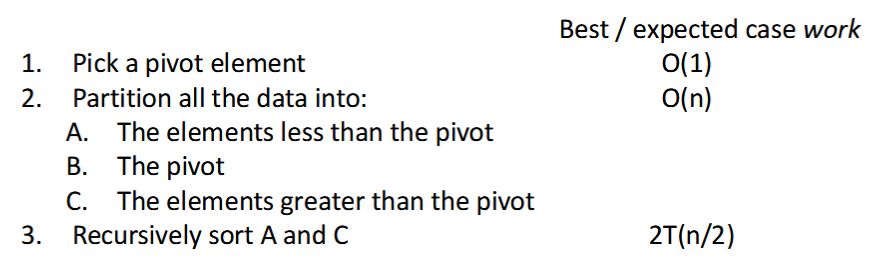
How can we parallelize Quicksort?
Back
How can we parallelize Quicksort?
Easy: Do the two recursive calls in parallel
- Work: unchanged of course \(O(n \log n)\)
- Span: now \(T(n) = O(n) + 1T(n/2) = O(n)\)
- So parallelism (i.e., work / span) is \(O(\log n)\)
After
Front
How can we parallelize Quicksort?
Back
How can we parallelize Quicksort?
Do the two recursive calls in parallel
- Work: unchanged of course \(O(n \log n)\)
- Span: now \(T(n) = O(n) + 1T(n/2) = O(n)\)
- So parallelism (i.e., work / span) is \(O(\log n)\)
Field-by-field Comparison
| Field | Before | After |
|---|---|---|
| Back | Do the two recursive calls in parallel <ul> <li>Work: unchanged of course \(O(n \log n)\)</li> <li>Span: now \(T(n) = O(n) + 1T(n/2) = O(n)\)</li> <li>So parallelism (i.e., work / span) is \(O(\log n)\)</li> </ul> |