Anki Deck Changes

Note 1: ETH::2. Semester::Analysis

Deck: ETH::2. Semester::Analysis
Note Type: Horvath Cloze
GUID: E#P*nHH>$>

modified

Before

Front

Sei $n \in \mathbb{N}$, $n \ge 1$. Dann hat die Gleichung $z^n = 1$ genau $n$ Lösungen in $\mathbb{C}$: $z_1, z_2, \dots, z_n$ wobei \[ z_j = {{c1:: \cos \frac{2\pi j}{n} + i \cdot \sin \frac{2 \pi j}{n} }}, \quad 1 \le j \le n \]

Back

Sei $n \in \mathbb{N}$, $n \ge 1$. Dann hat die Gleichung $z^n = 1$ genau $n$ Lösungen in $\mathbb{C}$: $z_1, z_2, \dots, z_n$ wobei \[ z_j = {{c1:: \cos \frac{2\pi j}{n} + i \cdot \sin \frac{2 \pi j}{n} }}, \quad 1 \le j \le n \]

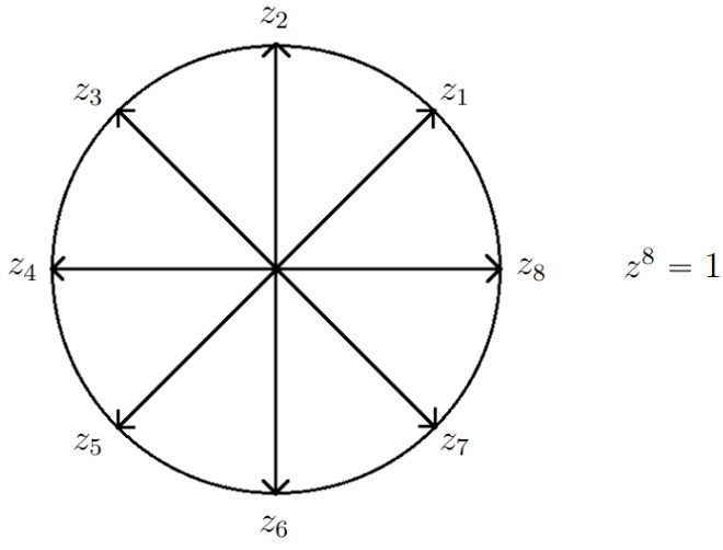
Die Lösungen sind alle auf einem Kreis mit Radius 1 und sind gleichmäßig verteilt (formen ein n-Eck).

Beispiel:

Für $w = R \cdot e^{i \varphi}$ sind die Lösungen von $z^n = w$ gleich der $n$ komplexen Zahlen mit Betrag $\sqrt[^n]{R}$ und Winkeln $\varphi_k = \frac{\varphi}{n} + k \cdot \frac{2 \pi}{n}$ für $k = 0, \dots, n - 1$.

After

Front

Sei $n \in \mathbb{N}$, $n \ge 1$.

Dann hat die Gleichung $z^n = 1$ genau $n$ Lösungen in $\mathbb{C}$: $z_1, z_2, \dots, z_n$ wobei: \[ z_j = {{c1:: \cos \frac{2\pi j}{n} + i \cdot \sin \frac{2 \pi j}{n} }}, \quad 1 \le j \le n \]

Back

Sei $n \in \mathbb{N}$, $n \ge 1$.

Dann hat die Gleichung $z^n = 1$ genau $n$ Lösungen in $\mathbb{C}$: $z_1, z_2, \dots, z_n$ wobei: \[ z_j = {{c1:: \cos \frac{2\pi j}{n} + i \cdot \sin \frac{2 \pi j}{n} }}, \quad 1 \le j \le n \]

Die Lösungen liegen alle auf einem Kreis mit Radius 1 und sind gleichmäßig verteilt (formen ein n-Eck).

Beispiel:

Für $w = R \cdot e^{i \varphi}$ sind die Lösungen von $z^n = w$ gleich der $n$ komplexen Zahlen mit Betrag $\sqrt[^n]{R}$ und Winkeln $\varphi_k = \frac{\varphi}{n} + k \cdot \frac{2 \pi}{n}$ für $k = 0, \dots, n - 1$.

Field-by-field Comparison

Field	Before	After
Text	Sei $n \in \mathbb{N}$, $n \ge 1$. Dann hat die Gleichung $z^n = 1$ genau $n$ Lösungen in $\mathbb{C}$: $z_1, z_2, \dots, z_n$ wobei \[ z_j = {{c1:: \cos \frac{2\pi j}{n} + i \cdot \sin \frac{2 \pi j}{n} }}, \quad 1 \le j \le n \]	Sei $n \in \mathbb{N}$, $n \ge 1$. <br><br>Dann hat die Gleichung $z^n = 1$ genau $n$ Lösungen in $\mathbb{C}$: $z_1, z_2, \dots, z_n$ wobei: \[ z_j = {{c1:: \cos \frac{2\pi j}{n} + i \cdot \sin \frac{2 \pi j}{n} }}, \quad 1 \le j \le n \]
Extra	<img src="paste-d82ffaf45ffbd9d16177968af1e2d0295676539b.jpg"><br><div>Die Lösungen ~~sind~~ alle auf einem Kreis mit Radius 1 und sind gleichmäßig verteilt (formen ein n-Eck).</div><div><br></div> <div>Beispiel: </div><div>Für $w = R \cdot e^{i \varphi}$ sind die Lösungen von $z^n = w$ gleich der $n$ komplexen Zahlen mit Betrag $\sqrt[^n]{R}$ und Winkeln $\varphi_k = \frac{\varphi}{n} + k \cdot \frac{2 \pi}{n}$ für $k = 0, \dots, n - 1$.</div>	<img src="paste-d82ffaf45ffbd9d16177968af1e2d0295676539b.jpg"><br><div>Die Lösungen liegen alle auf einem Kreis mit Radius 1 und sind gleichmäßig verteilt (formen ein n-Eck).</div><div><br></div> <div>Beispiel: </div><div>Für $w = R \cdot e^{i \varphi}$ sind die Lösungen von $z^n = w$ gleich der $n$ komplexen Zahlen mit Betrag $\sqrt[^n]{R}$ und Winkeln $\varphi_k = \frac{\varphi}{n} + k \cdot \frac{2 \pi}{n}$ für $k = 0, \dots, n - 1$.</div>

Tags: ETH::2._Semester::Analysis::1._Logik,_Mengen,_Zahlen::3._Zahlen::4._Komplexe_Zahlen::4._Einheitswurzeln

Note 2: ETH::2. Semester::Analysis

Deck: ETH::2. Semester::Analysis
Note Type: Horvath Cloze
GUID: M:f@_%USlo

modified

Before

Front

$\liminf_{n \rightarrow \infty} a_n$ ist der kleinste Häufungspunkt von $(a_n)$.
$\limsup_{n \rightarrow \infty} a_n$ ist der größte Häufungspunkt von $(a_n)$.

Back

$\liminf_{n \rightarrow \infty} a_n$ ist der kleinste Häufungspunkt von $(a_n)$.
$\limsup_{n \rightarrow \infty} a_n$ ist der größte Häufungspunkt von $(a_n)$.

(Limes inferior den kleinsten möglichen)

After

Front

$\liminf_{n \rightarrow \infty} a_n$ ist der kleinste Häufungspunkt von $(a_n)$.
$\limsup_{n \rightarrow \infty} a_n$ ist der größte Häufungspunkt von $(a_n)$.

Back

$\liminf_{n \rightarrow \infty} a_n$ ist der kleinste Häufungspunkt von $(a_n)$.
$\limsup_{n \rightarrow \infty} a_n$ ist der größte Häufungspunkt von $(a_n)$.

Field-by-field Comparison

Field	Before	After
Extra	~~(Limes inferior den kleinsten möglichen)~~

Tags: ETH::2._Semester::Analysis::2._Folgen::3._Häufungspunkte::2._Limsup_und_Liminf

Note 3: ETH::2. Semester::Analysis

Deck: ETH::2. Semester::Analysis
Note Type: Horvath Cloze
GUID: eaR`C4g=_B

modified

Before

Front

Eine Folge $(a_n)_{n \in \mathbb{N}_0} \subset \mathbb{R}$ heißt Cauchy-Folge, falls {{c1::für jedes $\epsilon > 0$ ein $N \in \mathbb{N}$ existiert, so dass gilt \[ \forall m, n \ge N \quad |a_n - a_m| < \epsilon \]}}

Back

Eine Folge $(a_n)_{n \in \mathbb{N}_0} \subset \mathbb{R}$ heißt Cauchy-Folge, falls {{c1::für jedes $\epsilon > 0$ ein $N \in \mathbb{N}$ existiert, so dass gilt \[ \forall m, n \ge N \quad |a_n - a_m| < \epsilon \]}}

Beispiel $\sum_{k = 1}^n \frac{1}{k^2}$ ist eine Cauchy Folge. Die Folge $\sum_{k = 1}^n \frac{1}{k}$ ist jedoch keine Cauchy-Folge.

After

Front

Eine Folge $(a_n)_{n \in \mathbb{N}_0} \subset \mathbb{R}$ heisst Cauchy-Folge, falls {{c1::für jedes $\epsilon > 0$ ein $N \in \mathbb{N}$ existiert, sodass gilt: \[ \forall m, n \ge N \quad |a_n - a_m| < \epsilon \]}}

Back

Eine Folge $(a_n)_{n \in \mathbb{N}_0} \subset \mathbb{R}$ heisst Cauchy-Folge, falls {{c1::für jedes $\epsilon > 0$ ein $N \in \mathbb{N}$ existiert, sodass gilt: \[ \forall m, n \ge N \quad |a_n - a_m| < \epsilon \]}}

Beispiele:
$\sum_{k = 1}^n \frac{1}{k^2}$ ist eine Cauchy Folge.
Die Folge $\sum_{k = 1}^n \frac{1}{k}$ ist hingegen keine Cauchy-Folge.

Field-by-field Comparison

Field	Before	After
Text	Eine Folge $(a_n)_{n \in \mathbb{N}_0} \subset \mathbb{R}$ heißt <b>Cauchy-Folge</b>, falls {{c1::für jedes $\epsilon > 0$ ein $N \in \mathbb{N}$ existiert, so dass gilt \[ \forall m, n \ge N \quad \|a_n - a_m\| < \epsilon \]}}	Eine Folge $(a_n)_{n \in \mathbb{N}_0} \subset \mathbb{R}$ heisst <b>Cauchy-Folge</b>, falls {{c1::für jedes $\epsilon > 0$ ein $N \in \mathbb{N}$ existiert, sodass gilt: \[ \forall m, n \ge N \quad \|a_n - a_m\| < \epsilon \]}}
Extra	<b>Beispiel</b> $\sum_{k = 1}^n \frac{1}{k^2}$ ist eine Cauchy Folge. Die Folge $\sum_{k = 1}^n \frac{1}{k}$ ist ~~jedoch~~ keine Cauchy-Folge.	<b>Beispiele:<br></b> $\sum_{k = 1}^n \frac{1}{k^2}$ ist eine Cauchy Folge. <br>Die Folge $\sum_{k = 1}^n \frac{1}{k}$ ist hingegen keine Cauchy-Folge.

Tags: ETH::2._Semester::Analysis::2._Folgen::2._Konvergenz::4._Cauchy_Folge

Note 4: ETH::2. Semester::Analysis

Deck: ETH::2. Semester::Analysis
Note Type: Horvath Cloze
GUID: f_B`=@^ngo

modified

Before

Front

Die Folge $\sup \{ a_k \mid k \ge n \}$ ist monoton fallend .

Back

Die Folge $\sup \{ a_k \mid k \ge n \}$ ist monoton fallend .

Für das infimum: monoton steigend.

Dies gilt, da $n = 2$ weniger Terme als $n = 1$ vergleicht (i.e. $\{a_k \mid k \ge n + 1\} \subseteq \{a_k \mid k \ge n\}$), deswegen kann es nur kleiner sein.

After

Front

Die Folge $\sup \{ a_k \mid k \ge n \}$ ist monoton fallend.

Back

Die Folge $\sup \{ a_k \mid k \ge n \}$ ist monoton fallend.

Für das Infinum: monoton steigend.

Dies gilt, da $n = 2$ weniger Terme als $n = 1$ vergleicht (d.h. $\{a_k \mid k \ge n + 1\} \subseteq \{a_k \mid k \ge n\}$), weswegen es nur kleiner sein kann.

Field-by-field Comparison

Field	Before	After
Text	Die Folge $\sup \{ a_k \mid k \ge n \}$ ist {{c1::monoton fallend :: property}}.	Die Folge $\sup \{ a_k \mid k \ge n \}$ ist {{c1::monoton fallend::property}}.
Extra	Für das infimum: monoton steigend.<br><br>Dies gilt, da $n = 2$ weniger Terme als $n = 1$ vergleicht (~~i.e~~. $\{a_k \mid k \ge n + 1\} \subseteq \{a_k \mid k \ge n\}$), deswegen ~~kann~~ es nur kleiner sein.	Für das Infinum: monoton steigend.<br><br>Dies gilt, da $n = 2$ weniger Terme als $n = 1$ vergleicht (d.h. $\{a_k \mid k \ge n + 1\} \subseteq \{a_k \mid k \ge n\}$), weswegen es nur kleiner sein kann.

Tags: ETH::2._Semester::Analysis::2._Folgen::3._Häufungspunkte::2._Limsup_und_Liminf

Note 5: ETH::2. Semester::Analysis

Deck: ETH::2. Semester::Analysis
Note Type: Horvath Classic
GUID: m?qT5<.33+

modified

Before

Front

Limes superior oder inferior können $\pm \infty$ sein?

Back

Limes superior oder inferior können $\pm \infty$ sein?

Ja

After

Front

Kann Limes superior (inferior) den Wert $+ \infty$ ($-\infty$) annehmen?

Back

Kann Limes superior (inferior) den Wert $+ \infty$ ($-\infty$) annehmen?

Ja.

Field-by-field Comparison

Field	Before	After
Front	Limes superior ~~oder~~ inferior ~~können $\pm~~ \infty$ ~~sei~~n?	Kann Limes superior (inferior) den Wert $+ \infty$ ($-\infty$) annehmen?
Back	Ja	Ja.

Tags: ETH::2._Semester::Analysis::2._Folgen::3._Häufungspunkte::2._Limsup_und_Liminf

Note 6: ETH::2. Semester::Analysis

Deck: ETH::2. Semester::Analysis
Note Type: Horvath Cloze
GUID: qu@PEalZbz

modified

Before

Front

Sandwich Theorem: Conditions for:
Dann ist auch die Folge $(b_n)_{n \in \mathbb{N}_0}$ konvergent und es gilt \[ \lim_{n \rightarrow \infty} b_n = L \]

Back

Sandwich Theorem: Conditions for:
Dann ist auch die Folge $(b_n)_{n \in \mathbb{N}_0}$ konvergent und es gilt \[ \lim_{n \rightarrow \infty} b_n = L \]

Es seien $(a_n)_{n \in \mathbb{N}_0}$ und $(c_n)_{n \in \mathbb{N}_0}$ zwei konvergente Folgen mit gleichem Grenzwert gegeben \[ \lim_{n \rightarrow \infty} a_n = L \text{ und } \lim_{n \rightarrow \infty} c_n = L \] sowie eine dritte Folge $(b_n)_{n \in \mathbb{N}_0}$ mit der Eigenschaft, dass ein $N_0 \in \mathbb{N}$ existiert, so dass gilt \[ a_n \le b_n \le c_n \quad \forall n \ge N_0 \]

After

Front

Es seien $(a_n)_{n \in \mathbb{N}_0}$ und $(c_n)_{n \in \mathbb{N}_0}$ zwei konvergente Folgen mit gleichem Grenzwert gegeben: \[ \lim_{n \rightarrow \infty} a_n = L \text{ und } \lim_{n \rightarrow \infty} c_n = L \] sowie eine dritte Folge $(b_n)_{n \in \mathbb{N}_0}$ mit der Eigenschaft, dass ein $N_0 \in \mathbb{N}$ existiert, so dass gilt:\[ a_n \le b_n \le c_n \quad \forall n \ge N_0 \] Dann ist die Folge $(b_n)_{n \in \mathbb{N}_0}$ konvergent und es gilt: \[ \lim_{n \rightarrow \infty} b_n = L \]

Back

Es seien $(a_n)_{n \in \mathbb{N}_0}$ und $(c_n)_{n \in \mathbb{N}_0}$ zwei konvergente Folgen mit gleichem Grenzwert gegeben: \[ \lim_{n \rightarrow \infty} a_n = L \text{ und } \lim_{n \rightarrow \infty} c_n = L \] sowie eine dritte Folge $(b_n)_{n \in \mathbb{N}_0}$ mit der Eigenschaft, dass ein $N_0 \in \mathbb{N}$ existiert, so dass gilt:\[ a_n \le b_n \le c_n \quad \forall n \ge N_0 \] Dann ist die Folge $(b_n)_{n \in \mathbb{N}_0}$ konvergent und es gilt: \[ \lim_{n \rightarrow \infty} b_n = L \]

(Sandwich-Theorem)

Field-by-field Comparison

Field	Before	After
Text	~~<b>Sandwich Theorem: </b>Conditions for:<br>~~Dann ist ~~auch~~ die Folge $(b_n)_{n \in \mathbb{N}_0}$ konvergent und es gilt \[ \lim_{n \rightarrow \infty} b_n = L \]<br>	Es seien $(a_n)_{n \in \mathbb{N}_0}$ und $(c_n)_{n \in \mathbb{N}_0}$ zwei konvergente Folgen mit gleichem Grenzwert gegeben: \[ \lim_{n \rightarrow \infty} a_n = L \text{ und } \lim_{n \rightarrow \infty} c_n = L \] sowie eine dritte Folge $(b_n)_{n \in \mathbb{N}_0}$ mit der Eigenschaft, dass ein $N_0 \in \mathbb{N}$ existiert, so dass gilt:\[ a_n \le b_n \le c_n \quad \forall n \ge N_0 \] Dann ist die Folge $(b_n)_{n \in \mathbb{N}_0}$ {{c1::konvergent}} und es gilt: \[ \lim_{n \rightarrow \infty} b_n = {{c1::L }}\]<br>
Extra	Es seien $(a_n)_{n \in \mathbb{N}_0}$ und $(c_n)_{n \in \mathbb{N}_0}$ zwei konvergente Folgen mit gleichem Grenzwert gegeben \[ \lim_{n \rightarrow \infty} a_n = L \text{ und } \lim_{n \rightarrow \infty} c_n = L \] sowie eine dritte Folge $(b_n)_{n \in \mathbb{N}_0}$ mit der Eigenschaft, dass ein $N_0 \in \mathbb{N}$ existiert, so dass gilt \[ a_n \le b_n \le c_n \quad \forall n \ge N_0 \] <br>	(Sandwich-Theorem)

Tags: ETH::2._Semester::Analysis::2._Folgen::2._Konvergenz::3._Kriterien

Note 7: ETH::2. Semester::Analysis

Deck: ETH::2. Semester::Analysis
Note Type: Horvath Cloze
GUID: r!b0]VV~/_

modified

Before

Front

Wenn $\lim a_n = 0$ eine Nullfolge ist, so gilt das du dumm bist, die implikation geht nur in eine Richtung.

Back

Wenn $\lim a_n = 0$ eine Nullfolge ist, so gilt das du dumm bist, die implikation geht nur in eine Richtung.

Ein Gegenbeispiel ist die Harmonische Reihe, $1/n $ ist eine Nullfolge, aber $\sum a_n$ konvergiert nicht.

After

Front

Wenn $\lim a_n = 0$ eine Nullfolge ist, so gilt, dass du dumm bist, die Implikation gilt nur in die Gegenrichtung.

Back

Wenn $\lim a_n = 0$ eine Nullfolge ist, so gilt, dass du dumm bist, die Implikation gilt nur in die Gegenrichtung.

Ein Gegenbeispiel ist die Harmonische Reihe, $1/n $ ist eine Nullfolge, aber $\sum a_n$ konvergiert nicht.

Field-by-field Comparison

Field	Before	After
Text	Wenn $\lim a_n = 0$ eine Nullfolge ist, so gilt {{c1:: ~~das~~ du dumm bist, die implikation geht nur in ~~eine R~~ichtung}}.	Wenn $\lim a_n = 0$ eine Nullfolge ist, so gilt, dass {{c1::du dumm bist, die Implikation gilt nur in die Gegenrichtung}}.
Extra	Ein Gegenbeispiel ist die Harmonische Reihe, $1/n $ ist eine Nullfolge, aber $\sum a_n$ konvergiert nicht.	<div style="text-align: center;"><img alt="Cat Laughing GIFs \| Tenor" src="cat-meme-laughing-gif.gif"></div><br>Ein Gegenbeispiel ist die Harmonische Reihe, $1/n $ ist eine Nullfolge, aber $\sum a_n$ konvergiert nicht.<br>

Tags: ETH::2._Semester::Analysis::3._Reihen

Note 8: ETH::2. Semester::Analysis

Deck: ETH::2. Semester::Analysis
Note Type: Horvath Classic
GUID: rgs$EaRM~}

modified

Before

Front

Trick: Rationalisieren

Back

Trick: Rationalisieren

Binomische Formel $a^2 - b^2 = (a - b)(a + b)$. Multipliziere die gleichung mit $\dots \times 1 = \dots \times \frac{\sqrt{n} + \sqrt{n + 1}}{\sqrt{n} - \sqrt{n + 1}}$ z.B. Beispiel: ${\sqrt{n^2 + 3} - n} \cdot 1 = \sqrt{n^2 + 3} - n \cdot \frac{\sqrt{n^2 + 3} + n}{\sqrt{n^2 + 3} + n}$ und dann mit $a^2 - b^2$ vereinfachen

After

Front

Trick: Rationalisieren

Back

Trick: Rationalisieren

Binomische Formel $a^2 - b^2 = (a - b)(a + b)$. Multipliziere die Gleichung mit $\dots \times 1 = \dots \times \frac{\sqrt{n} + \sqrt{n + 1}}{\sqrt{n} - \sqrt{n + 1}}$.

Beispiel: ${\sqrt{n^2 + 3} - n} \cdot 1 = \sqrt{n^2 + 3} - n \cdot \frac{\sqrt{n^2 + 3} + n}{\sqrt{n^2 + 3} + n}$ und dann mit $a^2 - b^2$ vereinfachen.

Field-by-field Comparison

Field	Before	After
Back	Binomische Formel $a^2 - b^2 = (a - b)(a + b)$. Multipliziere die gleichung mit $\dots \times 1 = \dots \times \frac{\sqrt{n} + \sqrt{n + 1}}{\sqrt{n} - \sqrt{n + 1}}$ ~~z.B.~~ <b>Beispiel:</b> ${\sqrt{n^2 + 3} - n} \cdot 1 = \sqrt{n^2 + 3} - n \cdot \frac{\sqrt{n^2 + 3} + n}{\sqrt{n^2 + 3} + n}$ und dann mit $a^2 - b^2$ vereinfachen	Binomische Formel $a^2 - b^2 = (a - b)(a + b)$. Multipliziere die Gleichung mit $\dots \times 1 = \dots \times \frac{\sqrt{n} + \sqrt{n + 1}}{\sqrt{n} - \sqrt{n + 1}}$. <br><b><br>Beispiel:</b> ${\sqrt{n^2 + 3} - n} \cdot 1 = \sqrt{n^2 + 3} - n \cdot \frac{\sqrt{n^2 + 3} + n}{\sqrt{n^2 + 3} + n}$ und dann mit $a^2 - b^2$ vereinfachen.

Tags: ETH::2._Semester::Analysis::2._Folgen::2._Konvergenz::5._Tricks

Note 9: ETH::2. Semester::Analysis

Deck: ETH::2. Semester::Analysis
Note Type: Horvath Classic
GUID: ssuChhYL(+

modified

Before

Front

Polarform (cosinus, sin) $z = re^{i \varphi} = $ schreiben.

Back

Polarform (cosinus, sin) $z = re^{i \varphi} = $ schreiben.

\[ e^x = 1 + x + \frac{x^2}{2} + \frac{x^3}{3!} + \dots = \sum_{k = 0}^\infty \frac{1}{k!}x^k \]Setzen wir in diese formel $x = it$ ein, so erhalten wir $e^{it} = \cos(t) + i \sin(t)$, $t \in \mathbb{R}$.

After

Front

Wie lautet $re^{i\varphi}$ ausgeschrieben mit $\cos$ und $\sin$?

Back

Wie lautet $re^{i\varphi}$ ausgeschrieben mit $\cos$ und $\sin$?

$re^{i \varphi} = r (\cos(\varphi) + i \sin(\varphi))$

Herleitung:\[ e^x = 1 + x + \frac{x^2}{2} + \frac{x^3}{3!} + \dots = \sum_{k = 0}^\infty \frac{1}{k!}x^k \]Setzen wir in diese formel $x = it$ ein, so erhalten wir $e^{it} = \cos(t) + i \sin(t)$, $t \in \mathbb{R}$.

Field-by-field Comparison

Field	Before	After
Front	~~Polarform (cosinus, sin)~~ $~~z =~~ re^{i \varphi} ~~= {{c1:: r (\cos(\varphi) + i \sin(\varphi)) }}$ schreiben.~~	Wie lautet $re^{i\varphi}$ ausgeschrieben mit $\cos$ und $\sin$?
Back	\[ e^x = 1 + x + \frac{x^2}{2} + \frac{x^3}{3!} + \dots = \sum_{k = 0}^\infty \frac{1}{k!}x^k \]Setzen wir in diese formel $x = it$ ein, so erhalten wir $e^{it} = \cos(t) + i \sin(t)$, $t \in \mathbb{R}$.	$re^{i \varphi} = r (\cos(\varphi) + i \sin(\varphi))$<br><br>Herleitung:\[ e^x = 1 + x + \frac{x^2}{2} + \frac{x^3}{3!} + \dots = \sum_{k = 0}^\infty \frac{1}{k!}x^k \]Setzen wir in diese formel $x = it$ ein, so erhalten wir $e^{it} = \cos(t) + i \sin(t)$, $t \in \mathbb{R}$.

Tags: ETH::2._Semester::Analysis::1._Logik,_Mengen,_Zahlen::3._Zahlen::4._Komplexe_Zahlen::3._Eulersche_Formel

Note 10: ETH::2. Semester::Analysis

Deck: ETH::2. Semester::Analysis
Note Type: Horvath Cloze
GUID: tRig1dSymm02

modified

Before

Front

\[ \cos(-\theta) = \cos\theta \] ($\cos$ is even)

Back

\[ \cos(-\theta) = \cos\theta \] ($\cos$ is even)

After

Front

\[ \cos(-\theta) = \cos\theta \]

Back

\[ \cos(-\theta) = \cos\theta \]

$\cos$ ist eine gerade Funktion.

Field-by-field Comparison

Field	Before	After
Text	\[ \cos(-\theta) = {{c1::\cos\theta}} \] ~~($\cos$ is {{c1::even}})~~	\[ \cos(-\theta) = {{c1::\cos\theta}} \]<br>
Extra		$\cos$ ist eine gerade Funktion.

Tags: ETH::2._Semester::Analysis::0._Trigonometrie::2._Identitäten::4._Symmetrie

Note 11: ETH::2. Semester::Analysis

Deck: ETH::2. Semester::Analysis
Note Type: Horvath Cloze
GUID: wje`U@*|!T

modified

Before

Front

Wenn $\sum a_n$ konvergiert, so gilt dass $\lim a_n = 0$ eine Nullfolge ist.

Back

Wenn $\sum a_n$ konvergiert, so gilt dass $\lim a_n = 0$ eine Nullfolge ist.

Das ist eine notwendige bedingung, nicht aber eine hinreichende.

After

Front

Wenn $\sum a_n$ konvergiert, so gilt, dass $\lim a_n = 0$ eine Nullfolge ist.

Back

Wenn $\sum a_n$ konvergiert, so gilt, dass $\lim a_n = 0$ eine Nullfolge ist.

Dies ist zwar eine notwendige Bedingung, jedoch noch keine hinreichende!

Field-by-field Comparison

Field	Before	After
Text	Wenn $\sum a_n$ konvergiert, so gilt {{c1:: ~~dass ~~$\lim a_n = 0$ eine Nullfolge ist}}.	Wenn $\sum a_n$ konvergiert, so gilt, dass {{c1::$\lim a_n = 0$ eine Nullfolge ist}}.
Extra	Das ist eine notwendige bedingung, nich~~t aber~~ eine hinreichende.	Dies ist zwar eine notwendige Bedingung, jedoch noch <b>keine hinreichende!</b>

Tags: ETH::2._Semester::Analysis::3._Reihen

Note 12: ETH::2. Semester::Analysis

Deck: ETH::2. Semester::Analysis
Note Type: Horvath Cloze
GUID: y~JMs{9f3

modified

Before

Front

Sei $(a_n)_{n \in \mathbb{N}_0}$ eine beschränkte Folge mit $A = \limsup_{n \rightarrow \infty} a_n$.
Dann ist $A$ ein Häufungspunkt und für alle $\epsilon > 0$ gilt,

Dass es nur endlich viele Elemente $a_n$ gibt, für welche gilt $a_n \ge A + \epsilon$
Dass für unendlich viele Element gilt $A - \epsilon < a_n < A + \epsilon$

Back

Sei $(a_n)_{n \in \mathbb{N}_0}$ eine beschränkte Folge mit $A = \limsup_{n \rightarrow \infty} a_n$.
Dann ist $A$ ein Häufungspunkt und für alle $\epsilon > 0$ gilt,

Dass es nur endlich viele Elemente $a_n$ gibt, für welche gilt $a_n \ge A + \epsilon$
Dass für unendlich viele Element gilt $A - \epsilon < a_n < A + \epsilon$

Eine analoge Aussage gilt auch für den limes inferior.

After

Front

Sei $(a_n)_{n \in \mathbb{N}_0}$ eine beschränkte Folge mit $A = \limsup_{n \rightarrow \infty} a_n$.
Dann ist $A$ ein Häufungspunkt und für alle $\epsilon > 0$ gilt, dass:

es nur endlich viele Elemente $a_n$ gibt, für welche $a_n \ge A + \epsilon$ gilt.
für unendlich viele Elemente $A - \epsilon < a_n < A + \epsilon$ gilt.

Back

Sei $(a_n)_{n \in \mathbb{N}_0}$ eine beschränkte Folge mit $A = \limsup_{n \rightarrow \infty} a_n$.
Dann ist $A$ ein Häufungspunkt und für alle $\epsilon > 0$ gilt, dass:

es nur endlich viele Elemente $a_n$ gibt, für welche $a_n \ge A + \epsilon$ gilt.
für unendlich viele Elemente $A - \epsilon < a_n < A + \epsilon$ gilt.

Eine analoge Aussage gilt auch für den Limes inferior.

Field-by-field Comparison

Field	Before	After
Text	Sei $(a_n)_{n \in \mathbb{N}_0}$ eine <i>beschränkte Folge</i> mit $A = \limsup_{n \rightarrow \infty} a_n$. <br>Dann ist $A$ ein <b>Häufungspunkt</b> und für alle $\epsilon > 0$ gilt, <br><ol><li>{{c1::~~Dass~~ es nur endlich viele Elemente $a_n$ gibt, für welche ~~gilt~~ $a_n \ge A + \epsilon$ }}</li><li>{{c2::~~Dass~~ für unendlich viele Element ~~gilt~~ $A - \epsilon < a_n < A + \epsilon$}}</li></ol>	Sei $(a_n)_{n \in \mathbb{N}_0}$ eine <i>beschränkte Folge</i> mit $A = \limsup_{n \rightarrow \infty} a_n$. <br>Dann ist $A$ ein <b>Häufungspunkt</b> und für alle $\epsilon > 0$ gilt, dass:<br><ol><li>{{c1::es nur endlich viele Elemente $a_n$ gibt, für welche $a_n \ge A + \epsilon$  gilt.}}</li><li>{{c2::für unendlich viele Elemente $A - \epsilon < a_n < A + \epsilon$ gilt.}}</li></ol>
Extra	Eine analoge Aussage gilt auch für den limes inferior.	Eine analoge Aussage gilt auch für den Limes inferior.

Tags: ETH::2._Semester::Analysis::2._Folgen::3._Häufungspunkte::2._Limsup_und_Liminf

Note 13: ETH::2. Semester::Analysis

Deck: ETH::2. Semester::Analysis
Note Type: Horvath Cloze
GUID: z!sAYo_L3D

modified

Before

Front

Für alle $P(n)$ polynome sodass $P(n) > 0$ gilt für große $n$: \[ \lim_{n \rightarrow \infty} \sqrt[n]{P(n)} = 1 \]

Back

Für alle $P(n)$ polynome sodass $P(n) > 0$ gilt für große $n$: \[ \lim_{n \rightarrow \infty} \sqrt[n]{P(n)} = 1 \]

Die Wurzel dämpft diese vollständig ab.

After

Front

Für alle Polynome $P(n)$ mit $P(n) > 0$, gilt für große $n$: \[ \lim_{n \rightarrow \infty} \sqrt[n]{P(n)} = 1 \]

Back

Für alle Polynome $P(n)$ mit $P(n) > 0$, gilt für große $n$: \[ \lim_{n \rightarrow \infty} \sqrt[n]{P(n)} = 1 \]

(Die Wurzel dämpft diese vollständig ab.)

Field-by-field Comparison

Field	Before	After
Text	Für alle ~~$P(n)$ polynome sodass~~ $P(n) > 0$ ~~gilt~~  für große $n$: \[ \lim_{n \rightarrow \infty} \sqrt[n]{P(n)} = {{c1:: 1}} \]	Für alle Polynome $P(n)$ mit $P(n) > 0$, gilt für große $n$: \[ \lim_{n \rightarrow \infty} \sqrt[n]{P(n)} = {{c1:: 1}} \]
Extra	Die Wurzel dämpft diese vollständig ab.	(Die Wurzel dämpft diese vollständig ab.)

Tags: ETH::2._Semester::Analysis::2._Folgen::1._Folgen::1._Properties

Note 14: ETH::2. Semester::PProg

Deck: ETH::2. Semester::PProg
Note Type: Horvath Classic
GUID: I[AczCve:{

modified

Before

Front

Considering Amdahl's Law, what limits the maximum Speedup?

Back

Considering Amdahl's Law, what limits the maximum Speedup?

The Sequential fraction of the program.

\[\lim_{P \to \infty} S_P \leq \frac{1}{f + \frac{1-f}{P}}\] \[\leq \frac{1}{f}\]

After

Front

Considering Amdahl's Law, what limits the maximum speedup?

Back

Considering Amdahl's Law, what limits the maximum speedup?

The sequential part of the program.

\[\lim_{P \to \infty} S_P \leq \frac{1}{f + \frac{1-f}{P}}\] \[\leq \frac{1}{f}\]

Field-by-field Comparison

Field	Before	After
Front	Considering Amdahl's Law, what limits the maximum Speedup?	Considering Amdahl's Law, what limits the maximum speedup?
Back	The Sequential ~~fraction~~ of the program.<br><br>\[\lim_{P \to \infty} S_P \leq \frac{1}{f + \frac{1-f}{P}}\] \[\leq \frac{1}{f}\]	The sequential part of the program.<br><br>\[\lim_{P \to \infty} S_P \leq \frac{1}{f + \frac{1-f}{P}}\] \[\leq \frac{1}{f}\]

Tags: ETH::2._Semester::PProg::07._Concepts::2._Parallel_performance

Note 15: ETH::2. Semester::PProg

Deck: ETH::2. Semester::PProg
Note Type: Horvath Cloze
GUID: I]N`CBnVud

modified

Before

Front

Amdahl's Law specifies the maximum amount of speedup that can be achieved for a program with a given sequential part. The pessimistic view on scalability.

Back

Amdahl's Law specifies the maximum amount of speedup that can be achieved for a program with a given sequential part. The pessimistic view on scalability.

After

Front

Amdahl's Law specifies the maximum amount of speedup that can be achieved for a program with a given sequential part.

Back

Amdahl's Law specifies the maximum amount of speedup that can be achieved for a program with a given sequential part.

The pessimistic view on scalability.

Field-by-field Comparison

Field	Before	After
Text	{{c1::Amdahl's Law}} specifies {{c2::the maximum amount of speedup}} that can be achieved for a program with a given sequential part. ~~The {{c3::pessimistic}} view on scalability.~~	{{c1::Amdahl's Law}} specifies {{c2::the maximum amount of speedup that can be achieved for a program with a given sequential part.}}
Extra		The pessimistic view on scalability.

Tags: ETH::2._Semester::PProg::07._Concepts::2._Parallel_performance ETH::2._Semester::PProg::Terminology

Note 16: ETH::2. Semester::PProg

Deck: ETH::2. Semester::PProg
Note Type: Horvath Cloze
GUID: LI8)TL2FuA

modified

Before

Front

Gustafson's Law looks at fixed time but increased problem size.

Back

Gustafson's Law looks at fixed time but increased problem size.

After

Front

Gustafson's Law looks at performance gains from the perspective of fixed time, but increased problem size.

Back

Gustafson's Law looks at performance gains from the perspective of fixed time, but increased problem size.

Field-by-field Comparison

Field	Before	After
Text	Gustafson's Law looks at {{c1::fixed time but increased problem size::what quantity, what variable}}.	Gustafson's Law looks at performance gains from the perspective of {{c1::fixed time, but increased problem size::what quantity, what variable}}.

Tags: ETH::2._Semester::PProg::07._Concepts::2._Parallel_performance

Note 17: ETH::2. Semester::PProg

Deck: ETH::2. Semester::PProg
Note Type: Horvath Cloze
GUID: w;6HF?V7OK

modified

Before

Front

Gustafson's Law specifies how much more work can be performed for a given fixed amount of time by adding more processors. The optimistic view on scalability.

Back

Gustafson's Law specifies how much more work can be performed for a given fixed amount of time by adding more processors. The optimistic view on scalability.

After

Front

Gustafson's Law specifies how much more work can be performed for a given fixed amount of time by adding more processors.

Back

Gustafson's Law specifies how much more work can be performed for a given fixed amount of time by adding more processors.

The optimistic view on scalability.

Field-by-field Comparison

Field	Before	After
Text	{{c1::Gustafson's Law}} specifies {{c2::how much more work can be performed}} for a given fixed amount of time by adding more processors. ~~The {{c3::optimistic view}} on scalability.~~	{{c1::Gustafson's Law}} specifies {{c2::how much more work can be performed for a given fixed amount of time by adding more processors.}}
Extra		The optimistic view on scalability.

Tags: ETH::2._Semester::PProg::Terminology ETH::2._Semester::PProg::07._Concepts::2._Parallel_performance

Field	Before	After
Text	Sei \(n \in \mathbb{N}\), \(n \ge 1\). Dann hat die Gleichung \(z^n = 1\) genau \(n\) Lösungen in \(\mathbb{C}\): \(z_1, z_2, \dots, z_n\) wobei \[ z_j = {{c1:: \cos \frac{2\pi j}{n} + i \cdot \sin \frac{2 \pi j}{n} }}, \quad 1 \le j \le n \]	Sei \(n \in \mathbb{N}\), \(n \ge 1\). <br><br>Dann hat die Gleichung \(z^n = 1\) genau \(n\) Lösungen in \(\mathbb{C}\): \(z_1, z_2, \dots, z_n\) wobei: \[ z_j = {{c1:: \cos \frac{2\pi j}{n} + i \cdot \sin \frac{2 \pi j}{n} }}, \quad 1 \le j \le n \]
Extra	<img src="paste-d82ffaf45ffbd9d16177968af1e2d0295676539b.jpg"><br><div>Die Lösungen ~~sind~~ alle auf einem Kreis mit Radius 1 und sind gleichmäßig verteilt (formen ein n-Eck).</div><div><br></div> <div>Beispiel: </div><div>Für \(w = R \cdot e^{i \varphi}\) sind die Lösungen von \(z^n = w\) gleich der \(n\) komplexen Zahlen mit Betrag \(\sqrt[^n]{R}\) und Winkeln \(\varphi_k = \frac{\varphi}{n} + k \cdot \frac{2 \pi}{n}\) für \(k = 0, \dots, n - 1\).</div>	<img src="paste-d82ffaf45ffbd9d16177968af1e2d0295676539b.jpg"><br><div>Die Lösungen liegen alle auf einem Kreis mit Radius 1 und sind gleichmäßig verteilt (formen ein n-Eck).</div><div><br></div> <div>Beispiel: </div><div>Für \(w = R \cdot e^{i \varphi}\) sind die Lösungen von \(z^n = w\) gleich der \(n\) komplexen Zahlen mit Betrag \(\sqrt[^n]{R}\) und Winkeln \(\varphi_k = \frac{\varphi}{n} + k \cdot \frac{2 \pi}{n}\) für \(k = 0, \dots, n - 1\).</div>

Field	Before	After
Text	Eine Folge \((a_n)_{n \in \mathbb{N}_0} \subset \mathbb{R}\) heißt <b>Cauchy-Folge</b>, falls {{c1::für jedes \(\epsilon > 0\) ein \(N \in \mathbb{N}\) existiert, so dass gilt \[ \forall m, n \ge N \quad \|a_n - a_m\| < \epsilon \]}}	Eine Folge \((a_n)_{n \in \mathbb{N}_0} \subset \mathbb{R}\) heisst <b>Cauchy-Folge</b>, falls {{c1::für jedes \(\epsilon > 0\) ein \(N \in \mathbb{N}\) existiert, sodass gilt: \[ \forall m, n \ge N \quad \|a_n - a_m\| < \epsilon \]}}
Extra	<b>Beispiel</b> \(\sum_{k = 1}^n \frac{1}{k^2}\) ist eine Cauchy Folge. Die Folge \(\sum_{k = 1}^n \frac{1}{k}\) ist ~~jedoch~~ keine Cauchy-Folge.	<b>Beispiele:<br></b> \(\sum_{k = 1}^n \frac{1}{k^2}\) ist eine Cauchy Folge. <br>Die Folge \(\sum_{k = 1}^n \frac{1}{k}\) ist hingegen keine Cauchy-Folge.

Field	Before	After
Text	Die Folge \(\sup \{ a_k \mid k \ge n \}\) ist {{c1::monoton fallend :: property}}.	Die Folge \(\sup \{ a_k \mid k \ge n \}\) ist {{c1::monoton fallend::property}}.
Extra	Für das infimum: monoton steigend.<br><br>Dies gilt, da \(n = 2\) weniger Terme als \(n = 1\) vergleicht (~~i.e~~. \(\{a_k \mid k \ge n + 1\} \subseteq \{a_k \mid k \ge n\}\)), deswegen ~~kann~~ es nur kleiner sein.	Für das Infinum: monoton steigend.<br><br>Dies gilt, da \(n = 2\) weniger Terme als \(n = 1\) vergleicht (d.h. \(\{a_k \mid k \ge n + 1\} \subseteq \{a_k \mid k \ge n\}\)), weswegen es nur kleiner sein kann.

Field	Before	After
Text	~~<b>Sandwich Theorem: </b>Conditions for:<br>~~Dann ist ~~auch~~ die Folge \((b_n)_{n \in \mathbb{N}_0}\) konvergent und es gilt \[ \lim_{n \rightarrow \infty} b_n = L \]<br>	Es seien \((a_n)_{n \in \mathbb{N}_0}\) und \((c_n)_{n \in \mathbb{N}_0}\) zwei konvergente Folgen mit gleichem Grenzwert gegeben: \[ \lim_{n \rightarrow \infty} a_n = L \text{ und } \lim_{n \rightarrow \infty} c_n = L \] sowie eine dritte Folge \((b_n)_{n \in \mathbb{N}_0}\) mit der Eigenschaft, dass ein \(N_0 \in \mathbb{N}\) existiert, so dass gilt:\[ a_n \le b_n \le c_n \quad \forall n \ge N_0 \] Dann ist die Folge \((b_n)_{n \in \mathbb{N}_0}\) {{c1::konvergent}} und es gilt: \[ \lim_{n \rightarrow \infty} b_n = {{c1::L }}\]<br>
Extra	Es seien \((a_n)_{n \in \mathbb{N}_0}\) und \((c_n)_{n \in \mathbb{N}_0}\) zwei konvergente Folgen mit gleichem Grenzwert gegeben \[ \lim_{n \rightarrow \infty} a_n = L \text{ und } \lim_{n \rightarrow \infty} c_n = L \] sowie eine dritte Folge \((b_n)_{n \in \mathbb{N}_0}\) mit der Eigenschaft, dass ein \(N_0 \in \mathbb{N}\) existiert, so dass gilt \[ a_n \le b_n \le c_n \quad \forall n \ge N_0 \] <br>	(Sandwich-Theorem)

Field	Before	After
Text	Wenn \(\lim a_n = 0\) eine Nullfolge ist, so gilt {{c1:: ~~das~~ du dumm bist, die implikation geht nur in ~~eine R~~ichtung}}.	Wenn \(\lim a_n = 0\) eine Nullfolge ist, so gilt, dass {{c1::du dumm bist, die Implikation gilt nur in die Gegenrichtung}}.
Extra	Ein Gegenbeispiel ist die Harmonische Reihe, \(1/n \) ist eine Nullfolge, aber \(\sum a_n\) konvergiert nicht.	<div style="text-align: center;"><img alt="Cat Laughing GIFs \| Tenor" src="cat-meme-laughing-gif.gif"></div><br>Ein Gegenbeispiel ist die Harmonische Reihe, \(1/n \) ist eine Nullfolge, aber \(\sum a_n\) konvergiert nicht.<br>

Field	Before	After
Front	~~Polarform (cosinus, sin)~~ \(~~z =~~ re^{i \varphi} ~~= {{c1:: r (\cos(\varphi) + i \sin(\varphi)) }}\) schreiben.~~	Wie lautet \(re^{i\varphi}\) ausgeschrieben mit \(\cos\) und \(\sin\)?
Back	\[ e^x = 1 + x + \frac{x^2}{2} + \frac{x^3}{3!} + \dots = \sum_{k = 0}^\infty \frac{1}{k!}x^k \]Setzen wir in diese formel \(x = it\) ein, so erhalten wir \(e^{it} = \cos(t) + i \sin(t)\), \(t \in \mathbb{R}\).	\(re^{i \varphi} = r (\cos(\varphi) + i \sin(\varphi))\)<br><br>Herleitung:\[ e^x = 1 + x + \frac{x^2}{2} + \frac{x^3}{3!} + \dots = \sum_{k = 0}^\infty \frac{1}{k!}x^k \]Setzen wir in diese formel \(x = it\) ein, so erhalten wir \(e^{it} = \cos(t) + i \sin(t)\), \(t \in \mathbb{R}\).

Field	Before	After
Text	Wenn \(\sum a_n\) konvergiert, so gilt {{c1:: ~~dass ~~\(\lim a_n = 0\) eine Nullfolge ist}}.	Wenn \(\sum a_n\) konvergiert, so gilt, dass {{c1::\(\lim a_n = 0\) eine Nullfolge ist}}.
Extra	Das ist eine notwendige bedingung, nich~~t aber~~ eine hinreichende.	Dies ist zwar eine notwendige Bedingung, jedoch noch <b>keine hinreichende!</b>

Field	Before	After
Text	Sei \((a_n)_{n \in \mathbb{N}_0}\) eine <i>beschränkte Folge</i> mit \(A = \limsup_{n \rightarrow \infty} a_n\). <br>Dann ist \(A\) ein <b>Häufungspunkt</b> und für alle \(\epsilon > 0\) gilt, <br><ol><li>{{c1::~~Dass~~ es nur endlich viele Elemente \(a_n\) gibt, für welche ~~gilt~~ \(a_n \ge A + \epsilon\) }}</li><li>{{c2::~~Dass~~ für unendlich viele Element ~~gilt~~ \(A - \epsilon < a_n < A + \epsilon\)}}</li></ol>	Sei \((a_n)_{n \in \mathbb{N}_0}\) eine <i>beschränkte Folge</i> mit \(A = \limsup_{n \rightarrow \infty} a_n\). <br>Dann ist \(A\) ein <b>Häufungspunkt</b> und für alle \(\epsilon > 0\) gilt, dass:<br><ol><li>{{c1::es nur endlich viele Elemente \(a_n\) gibt, für welche \(a_n \ge A + \epsilon\)  gilt.}}</li><li>{{c2::für unendlich viele Elemente \(A - \epsilon < a_n < A + \epsilon\) gilt.}}</li></ol>
Extra	Eine analoge Aussage gilt auch für den limes inferior.	Eine analoge Aussage gilt auch für den Limes inferior.

Field	Before	After
Text	Für alle ~~\(P(n)\) polynome sodass~~ \(P(n) > 0\) ~~gilt~~  für große \(n\): \[ \lim_{n \rightarrow \infty} \sqrt[n]{P(n)} = {{c1:: 1}} \]	Für alle Polynome \(P(n)\) mit \(P(n) > 0\), gilt für große \(n\): \[ \lim_{n \rightarrow \infty} \sqrt[n]{P(n)} = {{c1:: 1}} \]
Extra	Die Wurzel dämpft diese vollständig ab.	(Die Wurzel dämpft diese vollständig ab.)