Note 1: ETH::2. Semester::A&W
Deck: ETH::2. Semester::A&W
Note Type: Horvath Cloze
GUID: #k|8+%i6jy
added
Previous
Note did not exist
New Note
Front
ETH::2._Semester::A&W::3._Algorithmen_-_Highlights::1._Graphenalgorithmen::5._Konvexe_Hülle
Lokaler Verbesserungsschritt.
Gegeben \((q_0, q_1, \ldots, q_{k-1})\): Falls {{c1::\(q_{i+1}\) rechts von \(q_{i-1}, q_i\) liegt}}, dann entferne \(q_i\) aus der Folge.
Back
ETH::2._Semester::A&W::3._Algorithmen_-_Highlights::1._Graphenalgorithmen::5._Konvexe_Hülle
Lokaler Verbesserungsschritt.
Gegeben \((q_0, q_1, \ldots, q_{k-1})\): Falls {{c1::\(q_{i+1}\) rechts von \(q_{i-1}, q_i\) liegt}}, dann entferne \(q_i\) aus der Folge.
Genau die Verletzung der lokalen Konvexität (rechts statt links) macht \(q_i\) zu einer "Delle", die entfernt wird.
Field-by-field Comparison
| Field |
Before |
After |
| Text |
|
<b>Lokaler Verbesserungsschritt.</b><br>Gegeben \((q_0, q_1, \ldots, q_{k-1})\): Falls {{c1::\(q_{i+1}\) rechts von \(q_{i-1}, q_i\) liegt}}, dann {{c2::entferne \(q_i\) aus der Folge}}. |
| Extra |
|
Genau die Verletzung der lokalen Konvexität (rechts statt links) macht \(q_i\) zu einer "Delle", die entfernt wird. |
Tags:
ETH::2._Semester::A&W::3._Algorithmen_-_Highlights::1._Graphenalgorithmen::5._Konvexe_Hülle
Note 2: ETH::2. Semester::A&W
Deck: ETH::2. Semester::A&W
Note Type: Horvath Classic
GUID: *Rg2F@Ag#V
added
Previous
Note did not exist
New Note
Front
ETH::2._Semester::A&W::3._Algorithmen_-_Highlights::1._Graphenalgorithmen::4._Kleinster_umschliessender_Kreis::1._Grundlagen
Eindeutigkeit von \(C(P)\): Beweisidee.
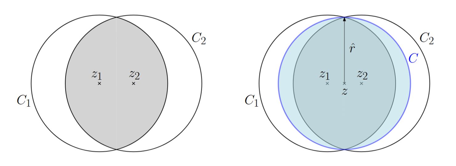
Angenommen, es gäbe zwei verschiedene kleinste umschliessende Kreise \(C_1, C_2\) mit gleichem Radius \(r\) und Mittelpunkten \(z_1 \neq z_2\).
Welchen kleineren Kreis konstruiert man als Widerspruch, und welchen Radius \(\hat r\) hat er?
Back
ETH::2._Semester::A&W::3._Algorithmen_-_Highlights::1._Graphenalgorithmen::4._Kleinster_umschliessender_Kreis::1._Grundlagen
Eindeutigkeit von \(C(P)\): Beweisidee.
Angenommen, es gäbe zwei verschiedene kleinste umschliessende Kreise \(C_1, C_2\) mit gleichem Radius \(r\) und Mittelpunkten \(z_1 \neq z_2\).
Welchen kleineren Kreis konstruiert man als Widerspruch, und welchen Radius \(\hat r\) hat er?
Da beide umschliessen, gilt \(P \subseteq C_1^{\bullet} \cap C_2^{\bullet}\).
Sei \(C\) der Kreis mit Mittelpunkt \(z = \tfrac{1}{2}(z_1 + z_2)\) (Mitte der Strecke \(z_1 z_2\)), und \(\hat r\) der Abstand von \(z\) zu den beiden Schnittpunkten von \(C_1\) und \(C_2\). Dann\[P \subseteq C_1^{\bullet} \cap C_2^{\bullet} \subseteq C^{\bullet}, \qquad \hat r = \sqrt{\,r^2 - \left(\tfrac{|z_1 z_2|}{2}\right)^2\,}.\]Wegen \(\hat r < r\) waren \(C_1, C_2\) keine kleinsten umschliessenden Kreise. Widerspruch.
Field-by-field Comparison
| Field |
Before |
After |
| Front |
|
<b>Eindeutigkeit von \(C(P)\): Beweisidee.<br></b><br>Angenommen, es gäbe zwei verschiedene kleinste umschliessende Kreise \(C_1, C_2\) mit gleichem Radius \(r\) und Mittelpunkten \(z_1 \neq z_2\). <br><br>Welchen kleineren Kreis konstruiert man als Widerspruch, und welchen Radius \(\hat r\) hat er? |
| Back |
|
Da beide umschliessen, gilt \(P \subseteq C_1^{\bullet} \cap C_2^{\bullet}\).<br>Sei \(C\) der Kreis mit Mittelpunkt \(z = \tfrac{1}{2}(z_1 + z_2)\) (Mitte der Strecke \(z_1 z_2\)), und \(\hat r\) der Abstand von \(z\) zu den beiden Schnittpunkten von \(C_1\) und \(C_2\). Dann\[P \subseteq C_1^{\bullet} \cap C_2^{\bullet} \subseteq C^{\bullet}, \qquad \hat r = \sqrt{\,r^2 - \left(\tfrac{|z_1 z_2|}{2}\right)^2\,}.\]Wegen \(\hat r < r\) waren \(C_1, C_2\) keine kleinsten umschliessenden Kreise. Widerspruch. |
Tags:
ETH::2._Semester::A&W::3._Algorithmen_-_Highlights::1._Graphenalgorithmen::4._Kleinster_umschliessender_Kreis::1._Grundlagen
Note 3: ETH::2. Semester::A&W
Deck: ETH::2. Semester::A&W
Note Type: Horvath Cloze
GUID: +ew>{IY~K_
added
Previous
Note did not exist
New Note
Front
ETH::2._Semester::A&W::3._Algorithmen_-_Highlights::1._Graphenalgorithmen::4._Kleinster_umschliessender_Kreis::4._Sampling_Lemma
Indikatorvariablen im Beweis des Sampling Lemmas.Für \(s \in P'\) und \(R, Q \subseteq P'\):
- \(\operatorname{out}(s, R) := 1\) genau dann, wenn {{c1::\(s \notin C^{\bullet}(R)\) (\(s\) liegt ausserhalb von \(C(R)\))}}.
- \(\operatorname{ess}(s, Q) := 1\) genau dann, wenn {{c2::\(C(Q \setminus \{s\}) \neq C(Q)\) (\(s\) ist essentiell für \(C(Q)\))}}.
Schlüsselbeziehung: \(\operatorname{out}(s, R) = 1 \iff {{c3::\operatorname{ess}(s, R \cup \{s\}) = 1}}\).
Back
ETH::2._Semester::A&W::3._Algorithmen_-_Highlights::1._Graphenalgorithmen::4._Kleinster_umschliessender_Kreis::4._Sampling_Lemma
Indikatorvariablen im Beweis des Sampling Lemmas.Für \(s \in P'\) und \(R, Q \subseteq P'\):
- \(\operatorname{out}(s, R) := 1\) genau dann, wenn {{c1::\(s \notin C^{\bullet}(R)\) (\(s\) liegt ausserhalb von \(C(R)\))}}.
- \(\operatorname{ess}(s, Q) := 1\) genau dann, wenn {{c2::\(C(Q \setminus \{s\}) \neq C(Q)\) (\(s\) ist essentiell für \(C(Q)\))}}.
Schlüsselbeziehung: \(\operatorname{out}(s, R) = 1 \iff {{c3::\operatorname{ess}(s, R \cup \{s\}) = 1}}\).
Ausserdem: \(\sum_{s \in P' \setminus R} \operatorname{out}(s, R) = |P' \setminus C^{\bullet}(R)|\) und \(\sum_{s \in Q} \operatorname{ess}(s, Q) \leq 3\) (höchstens 3 essentielle Punkte, vgl. kleine bestimmende Menge).
Field-by-field Comparison
| Field |
Before |
After |
| Text |
|
<b>Indikatorvariablen im Beweis des Sampling Lemmas.</b><br>Für \(s \in P'\) und \(R, Q \subseteq P'\):<br><ul><li>\(\operatorname{out}(s, R) := 1\) genau dann, wenn {{c1::\(s \notin C^{\bullet}(R)\) (\(s\) liegt ausserhalb von \(C(R)\))}}.</li><li>\(\operatorname{ess}(s, Q) := 1\) genau dann, wenn {{c2::\(C(Q \setminus \{s\}) \neq C(Q)\) (\(s\) ist essentiell für \(C(Q)\))}}.</li></ul>Schlüsselbeziehung: \(\operatorname{out}(s, R) = 1 \iff {{c3::\operatorname{ess}(s, R \cup \{s\}) = 1}}\). |
| Extra |
|
Ausserdem: \(\sum_{s \in P' \setminus R} \operatorname{out}(s, R) = |P' \setminus C^{\bullet}(R)|\) und \(\sum_{s \in Q} \operatorname{ess}(s, Q) \leq 3\) (höchstens 3 essentielle Punkte, vgl. kleine bestimmende Menge). |
Tags:
ETH::2._Semester::A&W::3._Algorithmen_-_Highlights::1._Graphenalgorithmen::4._Kleinster_umschliessender_Kreis::4._Sampling_Lemma
Note 4: ETH::2. Semester::A&W
Deck: ETH::2. Semester::A&W
Note Type: Horvath Classic
GUID: 2cIpbgekWL
modified
Before
Front
ETH::2._Semester::A&W::3._Algorithmen_-_Highlights::1._Graphenalgorithmen::3._Minimale_Schnitte_in_Graphen
Schreibe den modifizierten Algorithmus \(\textsc{Cut}_t(G)\), der die Kantenkontraktion bei \(t\) Knoten abbricht und dann einen randomisierten \(\mathcal{O}(t^4)\)-Algorithmus mit Erfolgswkt. \(\geq 1 - e^{-1}\) verwendet. Gib die untere Schranke für \(\hat{p}_t(n)\) und die resultierende Laufzeit nach \(\alpha / p_t(n)\)-maliger Wiederholung an.
Back
ETH::2._Semester::A&W::3._Algorithmen_-_Highlights::1._Graphenalgorithmen::3._Minimale_Schnitte_in_Graphen
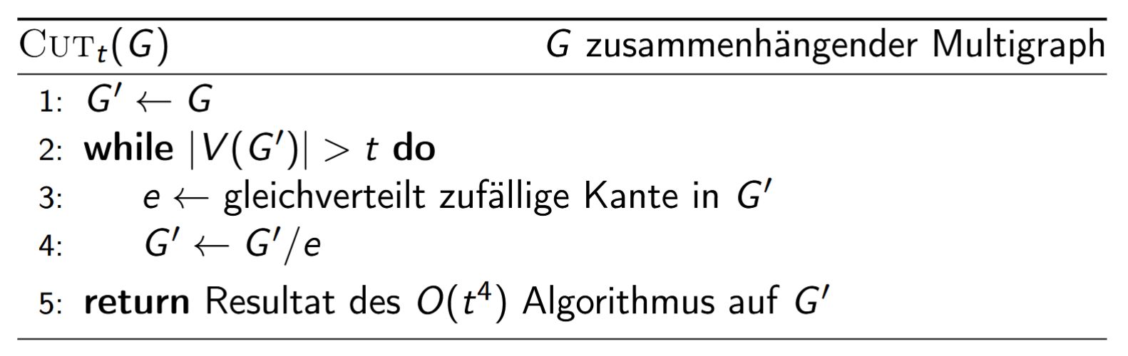
Schreibe den modifizierten Algorithmus \(\textsc{Cut}_t(G)\), der die Kantenkontraktion bei \(t\) Knoten abbricht und dann einen randomisierten \(\mathcal{O}(t^4)\)-Algorithmus mit Erfolgswkt. \(\geq 1 - e^{-1}\) verwendet. Gib die untere Schranke für \(\hat{p}_t(n)\) und die resultierende Laufzeit nach \(\alpha / p_t(n)\)-maliger Wiederholung an.
Cut_t(G)                     // G zus.hängender Multigraph
1: G' := G
2: while |V(G')| > t do
3:     e := gleichverteilt zufällige Kante in G'
4:     G' := G' / e
5: return Resultat des O(t^4) Algorithmus auf G'
Untere Schranke für die Erfolgswkt. einer Einzelausführung:\[\hat{p}_t(n) \;\geq\; \tfrac{n-2}{n} \cdot \tfrac{n-3}{n-1} \cdots \tfrac{t}{t+2} \cdot \tfrac{t-1}{t+1} \cdot \hat{p}_t(t) \;\geq\; \tfrac{t(t-1)}{n(n-1)} \cdot \tfrac{e-1}{e}.\]Nach \(\alpha / p_t(n)\)-maligem Wiederholen: Fehlerwkt. \(\leq e^{-\alpha}\) und Laufzeit\[\mathcal{O}\!\left(\alpha\!\left(\tfrac{n^4}{t^2} + n^2 t^2\right)\right).\]Wahl \(t := \sqrt{n}\) balanciert beide Terme und liefert \(\mathcal{O}(\alpha n^3)\).
After
Front
ETH::2._Semester::A&W::3._Algorithmen_-_Highlights::1._Graphenalgorithmen::3._Minimale_Schnitte_in_Graphen
Schreibe den modifizierten Algorithmus \(\text{Cut}_t(G)\), der die Kantenkontraktion bei \(t\) Knoten abbricht und dann einen randomisierten \(\mathcal{O}(t^4)\)-Algorithmus mit Erfolgswkt. \(\geq 1 - e^{-1}\) verwendet.
Gib die untere Schranke für \(\hat{p}_t(n)\) und die resultierende Laufzeit nach \(\alpha / p_t(n)\)-maliger Wiederholung an.
Back
ETH::2._Semester::A&W::3._Algorithmen_-_Highlights::1._Graphenalgorithmen::3._Minimale_Schnitte_in_Graphen
Schreibe den modifizierten Algorithmus \(\text{Cut}_t(G)\), der die Kantenkontraktion bei \(t\) Knoten abbricht und dann einen randomisierten \(\mathcal{O}(t^4)\)-Algorithmus mit Erfolgswkt. \(\geq 1 - e^{-1}\) verwendet.
Gib die untere Schranke für \(\hat{p}_t(n)\) und die resultierende Laufzeit nach \(\alpha / p_t(n)\)-maliger Wiederholung an.
Untere Schranke für die Erfolgswkt. einer Einzelausführung:\[\hat{p}_t(n) \;\geq\; \tfrac{n-2}{n} \cdot \tfrac{n-3}{n-1} \cdots \tfrac{t}{t+2} \cdot \tfrac{t-1}{t+1} \cdot \hat{p}_t(t) \;\geq\; \tfrac{t(t-1)}{n(n-1)} \cdot \tfrac{e-1}{e}.\]Nach \(\alpha / p_t(n)\)-maligem Wiederholen: Fehlerwkt. \(\leq e^{-\alpha}\) und Laufzeit\[\mathcal{O}\!\left(\alpha\!\left(\tfrac{n^4}{t^2} + n^2 t^2\right)\right).\]Wahl \(t := \sqrt{n}\) balanciert beide Terme und liefert \(\mathcal{O}(\alpha n^3)\).
Field-by-field Comparison
| Field |
Before |
After |
| Front |
Schreibe den modifizierten Algorithmus \(\textsc{Cut}_t(G)\), der die Kantenkontraktion bei \(t\) Knoten abbricht und dann einen randomisierten \(\mathcal{O}(t^4)\)-Algorithmus mit Erfolgswkt. \(\geq 1 - e^{-1}\) verwendet. Gib die untere Schranke für \(\hat{p}_t(n)\) und die resultierende Laufzeit nach \(\alpha / p_t(n)\)-maliger Wiederholung an. |
Schreibe den modifizierten Algorithmus \(\text{Cut}_t(G)\), der die Kantenkontraktion bei \(t\) Knoten abbricht und dann einen randomisierten \(\mathcal{O}(t^4)\)-Algorithmus mit Erfolgswkt. \(\geq 1 - e^{-1}\) verwendet. <br><br>Gib die untere Schranke für \(\hat{p}_t(n)\) und die resultierende Laufzeit nach \(\alpha / p_t(n)\)-maliger Wiederholung an. |
| Back |
<pre>Cut_t(G) // G zus.hängender Multigraph
1: G' := G
2: while |V(G')| > t do
3: e := gleichverteilt zufällige Kante in G'
4: G' := G' / e
5: return Resultat des O(t^4) Algorithmus auf G'</pre>Untere Schranke für die Erfolgswkt. einer Einzelausführung:\[\hat{p}_t(n) \;\geq\; \tfrac{n-2}{n} \cdot \tfrac{n-3}{n-1} \cdots \tfrac{t}{t+2} \cdot \tfrac{t-1}{t+1} \cdot \hat{p}_t(t) \;\geq\; \tfrac{t(t-1)}{n(n-1)} \cdot \tfrac{e-1}{e}.\]Nach \(\alpha / p_t(n)\)-maligem Wiederholen: Fehlerwkt. \(\leq e^{-\alpha}\) und Laufzeit\[\mathcal{O}\!\left(\alpha\!\left(\tfrac{n^4}{t^2} + n^2 t^2\right)\right).\]Wahl \(t := \sqrt{n}\) balanciert beide Terme und liefert \(\mathcal{O}(\alpha n^3)\). |
<img src="paste-13d74473ba09dba05a8c2d0f27aa5dd3b4c906c8.jpg"><br><br>Untere Schranke für die Erfolgswkt. einer Einzelausführung:\[\hat{p}_t(n) \;\geq\; \tfrac{n-2}{n} \cdot \tfrac{n-3}{n-1} \cdots \tfrac{t}{t+2} \cdot \tfrac{t-1}{t+1} \cdot \hat{p}_t(t) \;\geq\; \tfrac{t(t-1)}{n(n-1)} \cdot \tfrac{e-1}{e}.\]Nach \(\alpha / p_t(n)\)-maligem Wiederholen: Fehlerwkt. \(\leq e^{-\alpha}\) und Laufzeit\[\mathcal{O}\!\left(\alpha\!\left(\tfrac{n^4}{t^2} + n^2 t^2\right)\right).\]Wahl \(t := \sqrt{n}\) balanciert beide Terme und liefert \(\mathcal{O}(\alpha n^3)\).<br> |
Tags:
ETH::2._Semester::A&W::3._Algorithmen_-_Highlights::1._Graphenalgorithmen::3._Minimale_Schnitte_in_Graphen
Note 5: ETH::2. Semester::A&W
Deck: ETH::2. Semester::A&W
Note Type: Horvath Classic
GUID: 55>>G~C,D{
added
Previous
Note did not exist
New Note
Front
ETH::2._Semester::A&W::3._Algorithmen_-_Highlights::1._Graphenalgorithmen::4._Kleinster_umschliessender_Kreis::4._Sampling_Lemma
Sampling Lemma: Beweis (Kernrechnung).
Wie kommt man von \(\mathbb{E}[|P' \setminus C^{\bullet}(R)|]\) auf die Schranke \(3\,\frac{N-r}{r+1}\)? (Stichworte: out/ess, Wechsel \(R \to Q\).)
Back
ETH::2._Semester::A&W::3._Algorithmen_-_Highlights::1._Graphenalgorithmen::4._Kleinster_umschliessender_Kreis::4._Sampling_Lemma
Sampling Lemma: Beweis (Kernrechnung).
Wie kommt man von \(\mathbb{E}[|P' \setminus C^{\bullet}(R)|]\) auf die Schranke \(3\,\frac{N-r}{r+1}\)? (Stichworte: out/ess, Wechsel \(R \to Q\).)
\[\begin{gathered}\mathbb{E}\big[|P' \setminus C^{\bullet}(R)|\big] = \frac{1}{\binom{N}{r}} \sum_{R \in \binom{P'}{r}} \sum_{s \in P' \setminus R} \operatorname{out}(s, R) \\= \frac{1}{\binom{N}{r}} \sum_{R \in \binom{P'}{r}} \sum_{s \in P' \setminus R} \operatorname{ess}(s, R \cup \{s\}) \\= \frac{1}{\binom{N}{r}} \sum_{Q \in \binom{P'}{r+1}} \underbrace{\sum_{s \in Q} \operatorname{ess}(s, Q)}_{\leq 3} \;\leq\; \frac{3 \binom{N}{r+1}}{\binom{N}{r}} = 3\,\frac{N - r}{r + 1}.\end{gathered}\]Der mittlere Schritt nutzt \(\operatorname{out}(s,R) = \operatorname{ess}(s, R\cup\{s\})\); danach fasst man Paare \((R, s)\) zu \(Q = R \cup \{s\}\) der Grösse \(r+1\) zusammen.
Field-by-field Comparison
| Field |
Before |
After |
| Front |
|
<b>Sampling Lemma: Beweis (Kernrechnung).</b><br>Wie kommt man von \(\mathbb{E}[|P' \setminus C^{\bullet}(R)|]\) auf die Schranke \(3\,\frac{N-r}{r+1}\)? (Stichworte: out/ess, Wechsel \(R \to Q\).) |
| Back |
|
\[\begin{gathered}\mathbb{E}\big[|P' \setminus C^{\bullet}(R)|\big] = \frac{1}{\binom{N}{r}} \sum_{R \in \binom{P'}{r}} \sum_{s \in P' \setminus R} \operatorname{out}(s, R) \\= \frac{1}{\binom{N}{r}} \sum_{R \in \binom{P'}{r}} \sum_{s \in P' \setminus R} \operatorname{ess}(s, R \cup \{s\}) \\= \frac{1}{\binom{N}{r}} \sum_{Q \in \binom{P'}{r+1}} \underbrace{\sum_{s \in Q} \operatorname{ess}(s, Q)}_{\leq 3} \;\leq\; \frac{3 \binom{N}{r+1}}{\binom{N}{r}} = 3\,\frac{N - r}{r + 1}.\end{gathered}\]Der mittlere Schritt nutzt \(\operatorname{out}(s,R) = \operatorname{ess}(s, R\cup\{s\})\); danach fasst man Paare \((R, s)\) zu \(Q = R \cup \{s\}\) der Grösse \(r+1\) zusammen. |
Tags:
ETH::2._Semester::A&W::3._Algorithmen_-_Highlights::1._Graphenalgorithmen::4._Kleinster_umschliessender_Kreis::4._Sampling_Lemma
Note 6: ETH::2. Semester::A&W
Deck: ETH::2. Semester::A&W
Note Type: Horvath Cloze
GUID: 8sQ[?skk.]
added
Previous
Note did not exist
New Note
Front
ETH::2._Semester::A&W::3._Algorithmen_-_Highlights::1._Graphenalgorithmen::5._Konvexe_Hülle
Das Startpolygon für LocalRepair.
Sortiere \(P\) aufsteigend nach \(x\)-Koordinate zu \((p_1, p_2, \ldots, p_n)\) und betrachte das Polygon \[{{c1::(p_1, p_2, \ldots, p_{n-1}, p_n, p_{n-1}, \ldots, p_2)}}.\]Es hat \(2(n-1)\) Ecken und durchläuft die Punkte einmal hin (unten) und einmal zurück (oben).
Back
ETH::2._Semester::A&W::3._Algorithmen_-_Highlights::1._Graphenalgorithmen::5._Konvexe_Hülle
Das Startpolygon für LocalRepair.
Sortiere \(P\) aufsteigend nach \(x\)-Koordinate zu \((p_1, p_2, \ldots, p_n)\) und betrachte das Polygon \[{{c1::(p_1, p_2, \ldots, p_{n-1}, p_n, p_{n-1}, \ldots, p_2)}}.\]Es hat \(2(n-1)\) Ecken und durchläuft die Punkte einmal hin (unten) und einmal zurück (oben).
Field-by-field Comparison
| Field |
Before |
After |
| Text |
|
<b>Das Startpolygon für LocalRepair.</b><br>Sortiere \(P\) aufsteigend nach \(x\)-Koordinate zu \((p_1, p_2, \ldots, p_n)\) und betrachte das Polygon \[{{c1::(p_1, p_2, \ldots, p_{n-1}, p_n, p_{n-1}, \ldots, p_2)}}.\]Es hat {{c2::\(2(n-1)\)}} Ecken und durchläuft die Punkte einmal hin (unten) und einmal zurück (oben). |
Tags:
ETH::2._Semester::A&W::3._Algorithmen_-_Highlights::1._Graphenalgorithmen::5._Konvexe_Hülle
Note 7: ETH::2. Semester::A&W
Deck: ETH::2. Semester::A&W
Note Type: Horvath Classic
GUID: ;/-rm%9`[`
added
Previous
Note did not exist
New Note
Front
ETH::2._Semester::A&W::3._Algorithmen_-_Highlights::1._Graphenalgorithmen::5._Konvexe_Hülle
Defizite der rein lokalen Konvexitätsbedingung.
Welche drei unerwünschten Situationen schliesst die lokale Bedingung \(q_{i+1}\) links von \(q_{i-1}, q_i\) allein noch nicht aus?
Back
ETH::2._Semester::A&W::3._Algorithmen_-_Highlights::1._Graphenalgorithmen::5._Konvexe_Hülle
Defizite der rein lokalen Konvexitätsbedingung.
Welche drei unerwünschten Situationen schliesst die lokale Bedingung \(q_{i+1}\) links von \(q_{i-1}, q_i\) allein noch nicht aus?
- \(\{q_0, \ldots, q_{h-1}\}\) muss keine Teilmenge von \(P\) sein.
- Das Polygon muss nicht alle anderen Punkte im Inneren haben.
- Das Polygon kann sich selbst kreuzen.
Idee: Mit einem geeigneten (nicht notwendig konvexen) Startpolygon, das die lokale Bedingung nicht verletzt, sukzessive "konvexifizieren" (lokal verbessern).
Field-by-field Comparison
| Field |
Before |
After |
| Front |
|
<b>Defizite der rein lokalen Konvexitätsbedingung.</b><br>Welche drei unerwünschten Situationen schliesst die lokale Bedingung \(q_{i+1}\) links von \(q_{i-1}, q_i\) <b>allein</b> noch nicht aus? |
| Back |
|
<ul><li>\(\{q_0, \ldots, q_{h-1}\}\) muss keine Teilmenge von \(P\) sein.</li><li>Das Polygon muss nicht alle anderen Punkte im Inneren haben.</li><li>Das Polygon kann sich selbst kreuzen.</li></ul>Idee: Mit einem geeigneten (nicht notwendig konvexen) Startpolygon, das die lokale Bedingung nicht verletzt, sukzessive "konvexifizieren" (lokal verbessern). |
Tags:
ETH::2._Semester::A&W::3._Algorithmen_-_Highlights::1._Graphenalgorithmen::5._Konvexe_Hülle
Note 8: ETH::2. Semester::A&W
Deck: ETH::2. Semester::A&W
Note Type: Horvath Classic
GUID: ?y[w6OEt^}
modified
Before
Front
ETH::2._Semester::A&W::3._Algorithmen_-_Highlights::1._Graphenalgorithmen::3._Minimale_Schnitte_in_Graphen
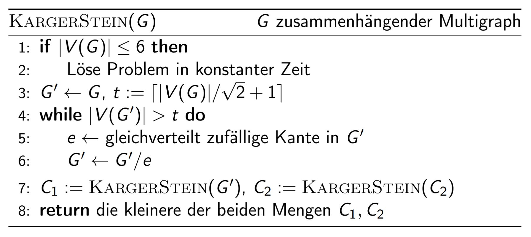
Schreibe den Karger-Stein-Algorithmus als rekursiven Pseudocode.
Back
ETH::2._Semester::A&W::3._Algorithmen_-_Highlights::1._Graphenalgorithmen::3._Minimale_Schnitte_in_Graphen
Schreibe den Karger-Stein-Algorithmus als rekursiven Pseudocode.
KargerStein(G)               // G zus.hängender Multigraph
1: if |V(G)| <= 6 then
2:     Löse Problem in konstanter Zeit
3: G' := G,  t := ceil(|V(G)| / sqrt(2) + 1)
4: while |V(G')| > t do
5:     e := gleichverteilt zufällige Kante in G'
6:     G' := G' / e
7: C_1 := KargerStein(G')
8: C_2 := KargerStein(G')         // zweiter, unabhängiger Rekursionsast
9: return die kleinere der beiden Mengen C_1, C_2
Die Wahl \(t \approx n/\sqrt{2}\) garantiert, dass die Erfolgswkt. eines einzelnen Asts (\(n \to t\) Knoten) konstant ist; durch
zwei unabhängige rekursive Aufrufe wird die Misserfolgswkt. quadriert, was den Gesamtfehler beherrschbar hält. Resultierende Laufzeit: \(\mathcal{O}(n^2 \log n)\), Erfolgswkt. \(\Omega(1/\log n)\); nach \(\Theta(\log^2 n)\) Wiederholungen Fehlerwkt. \(\leq 1/n\).
After
Front
ETH::2._Semester::A&W::3._Algorithmen_-_Highlights::1._Graphenalgorithmen::3._Minimale_Schnitte_in_Graphen
Schreibe den Karger-Stein-Algorithmus als rekursiven Pseudocode.
Back
ETH::2._Semester::A&W::3._Algorithmen_-_Highlights::1._Graphenalgorithmen::3._Minimale_Schnitte_in_Graphen
Schreibe den Karger-Stein-Algorithmus als rekursiven Pseudocode.
Die Wahl \(t \approx n/\sqrt{2}\) garantiert, dass die Erfolgswkt. eines einzelnen Asts (\(n \to t\) Knoten) konstant ist; durch
zwei unabhängige rekursive Aufrufe wird die Misserfolgswkt. quadriert, was den Gesamtfehler beherrschbar hält.
Resultierende Laufzeit: \(\mathcal{O}(n^2 \log n)\), Erfolgswkt. \(\Omega(1/\log n)\); nach \(\Theta(\log^2 n)\) Wiederholungen Fehlerwkt. \(\leq 1/n\).
Field-by-field Comparison
| Field |
Before |
After |
| Back |
<pre>KargerStein(G) // G zus.hängender Multigraph
1: if |V(G)| <= 6 then
2: Löse Problem in konstanter Zeit
3: G' := G, t := ceil(|V(G)| / sqrt(2) + 1)
4: while |V(G')| > t do
5: e := gleichverteilt zufällige Kante in G'
6: G' := G' / e
7: C_1 := KargerStein(G')
8: C_2 := KargerStein(G') // zweiter, unabhängiger Rekursionsast
9: return die kleinere der beiden Mengen C_1, C_2</pre>Die Wahl \(t \approx n/\sqrt{2}\) garantiert, dass die Erfolgswkt. eines einzelnen Asts (\(n \to t\) Knoten) konstant ist; durch <b>zwei unabhängige rekursive Aufrufe</b> wird die Misserfolgswkt. quadriert, was den Gesamtfehler beherrschbar hält. Resultierende Laufzeit: \(\mathcal{O}(n^2 \log n)\), Erfolgswkt. \(\Omega(1/\log n)\); nach \(\Theta(\log^2 n)\) Wiederholungen Fehlerwkt. \(\leq 1/n\). |
<img src="paste-cab04964f94ce816c352802382a38a9aec930d0a.jpg"><br><br>Die Wahl \(t \approx n/\sqrt{2}\) garantiert, dass die Erfolgswkt. eines einzelnen Asts (\(n \to t\) Knoten) konstant ist; durch <b>zwei unabhängige rekursive Aufrufe</b> wird die Misserfolgswkt. quadriert, was den Gesamtfehler beherrschbar hält. <br><br>Resultierende Laufzeit: \(\mathcal{O}(n^2 \log n)\), Erfolgswkt. \(\Omega(1/\log n)\); nach \(\Theta(\log^2 n)\) Wiederholungen Fehlerwkt. \(\leq 1/n\). |
Tags:
ETH::2._Semester::A&W::3._Algorithmen_-_Highlights::1._Graphenalgorithmen::3._Minimale_Schnitte_in_Graphen
Note 9: ETH::2. Semester::A&W
Deck: ETH::2. Semester::A&W
Note Type: Horvath Classic
GUID: D/A{W?@*_o
modified
Before
Front
ETH::2._Semester::A&W::1._Graphentheorie::7._Färbungen ETH::2._Semester::A&W::Minitests::2
Wahr oder falsch?
Jeder Kreis ist 2-färbbar.
Back
ETH::2._Semester::A&W::1._Graphentheorie::7._Färbungen ETH::2._Semester::A&W::Minitests::2
Wahr oder falsch?
Jeder Kreis ist 2-färbbar.
Falsch
After
Front
ETH::2._Semester::A&W::1._Graphentheorie::7._Färbungen ETH::2._Semester::A&W::Minitests::2
Wahr oder falsch?
Jeder Kreis ist 2-färbbar.
Back
ETH::2._Semester::A&W::1._Graphentheorie::7._Färbungen ETH::2._Semester::A&W::Minitests::2
Wahr oder falsch?
Jeder Kreis ist 2-färbbar.
Falsch.
Field-by-field Comparison
| Field |
Before |
After |
| Back |
Falsch |
Falsch. |
Tags:
ETH::2._Semester::A&W::1._Graphentheorie::7._Färbungen
ETH::2._Semester::A&W::Minitests::2
Note 10: ETH::2. Semester::A&W
Deck: ETH::2. Semester::A&W
Note Type: Horvath Cloze
GUID: G=p3gO|{IJ
added
Previous
Note did not exist
New Note
Front
ETH::2._Semester::A&W::3._Algorithmen_-_Highlights::1._Graphenalgorithmen::5._Konvexe_Hülle
Randkante.
Ein Paar \(qr \in P^2\), \(q \neq r\), heisst Randkante von \(P\), falls {{c1::alle Punkte in \(P \setminus \{q, r\}\) links von \(q, r\) liegen}} (d.h. auf der linken Seite der von \(q\) nach \(r\) gerichteten Geraden).
Back
ETH::2._Semester::A&W::3._Algorithmen_-_Highlights::1._Graphenalgorithmen::5._Konvexe_Hülle
Randkante.
Ein Paar \(qr \in P^2\), \(q \neq r\), heisst Randkante von \(P\), falls {{c1::alle Punkte in \(P \setminus \{q, r\}\) links von \(q, r\) liegen}} (d.h. auf der linken Seite der von \(q\) nach \(r\) gerichteten Geraden).
Diese gerichtete Sichtweise legt direkt die Gegen-Uhrzeigersinn-Orientierung der Hülle fest.
Field-by-field Comparison
| Field |
Before |
After |
| Text |
|
<b>Randkante.</b><br>Ein Paar \(qr \in P^2\), \(q \neq r\), heisst <b>Randkante</b> von \(P\), falls {{c1::alle Punkte in \(P \setminus \{q, r\}\) links von \(q, r\) liegen}} (d.h. auf der linken Seite der von \(q\) nach \(r\) gerichteten Geraden). |
| Extra |
|
Diese gerichtete Sichtweise legt direkt die Gegen-Uhrzeigersinn-Orientierung der Hülle fest. |
Tags:
ETH::2._Semester::A&W::3._Algorithmen_-_Highlights::1._Graphenalgorithmen::5._Konvexe_Hülle
Note 11: ETH::2. Semester::A&W
Deck: ETH::2. Semester::A&W
Note Type: Horvath Cloze
GUID: GUSRKOlJ(I
modified
Before
Front
ETH::2._Semester::A&W::2._Wahrscheinlichkeitstheorie_und_randomisierte_Algorithmen::8._Randomisierte_Algorithmen::3._Primzahltest
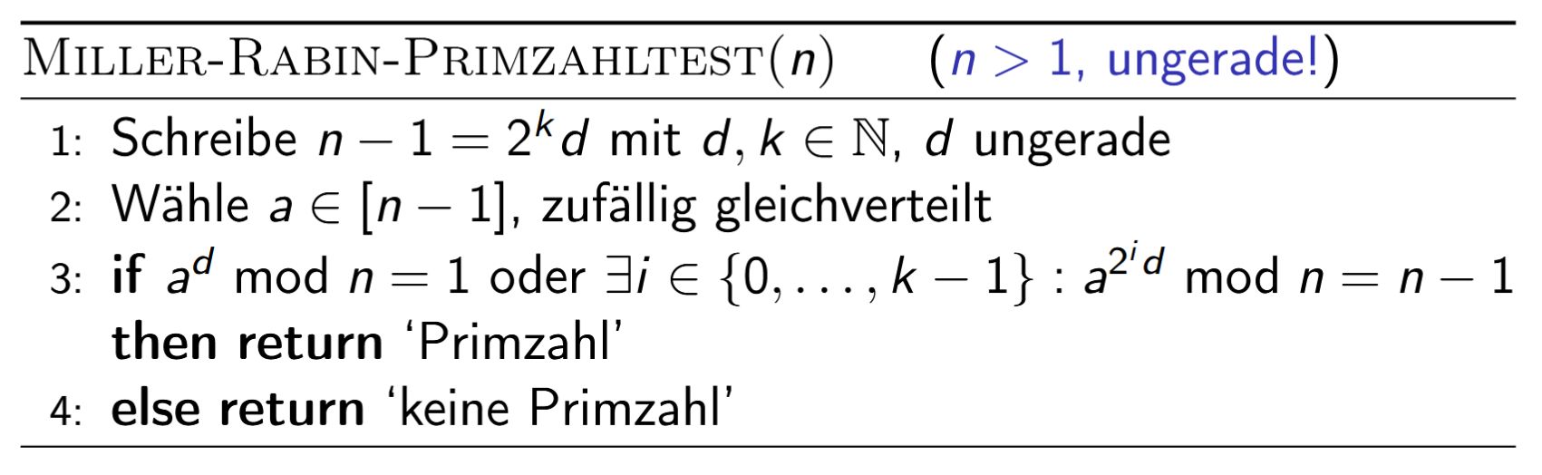
Miller-Rabin-Primzahltest (für \(n > 1\) ungerade):
1. Schreibe n - 1 = 2^k · d mit d ungerade
2. Wähle a ∈ [n-1] zufällig gleichverteilt
3. if a^d mod n = 1
   oder ∃i ∈ {0,...,k-1}: a^(2^i·d) mod n = n-1:
     return 'Primzahl'
   else:
     return 'keine Primzahl'
Korrektheit:
- Falls \(n\) prim: Ausgabe immer korrekt.
- Falls \(n\) nicht prim: Falsche Ausgabe 'Primzahl' mit Wahrscheinlichkeit {{c2::\(\leq \tfrac{1}{2}\), tatsächlich sogar \(\leq \tfrac{1}{4}\)}}.
Back
ETH::2._Semester::A&W::2._Wahrscheinlichkeitstheorie_und_randomisierte_Algorithmen::8._Randomisierte_Algorithmen::3._Primzahltest
Miller-Rabin-Primzahltest (für \(n > 1\) ungerade):
1. Schreibe n - 1 = 2^k · d mit d ungerade
2. Wähle a ∈ [n-1] zufällig gleichverteilt
3. if a^d mod n = 1
   oder ∃i ∈ {0,...,k-1}: a^(2^i·d) mod n = n-1:
     return 'Primzahl'
   else:
     return 'keine Primzahl'
Korrektheit:
- Falls \(n\) prim: Ausgabe immer korrekt.
- Falls \(n\) nicht prim: Falsche Ausgabe 'Primzahl' mit Wahrscheinlichkeit {{c2::\(\leq \tfrac{1}{2}\), tatsächlich sogar \(\leq \tfrac{1}{4}\)}}.
Im Gegensatz zum Fermat-Test funktioniert Miller-Rabin auch für Carmichael-Zahlen.
Beispiel \(n = 561\) mit \(a = 2\):
\(n - 1 = 560 = 2^4 \cdot 35\),
und \(2^{280} \equiv_{561} 1\),
aber \(2^{140} \equiv_{561} 67 \notin \{1, 560\}\).
Also ist \(2\) ein Miller-Rabin-Zertifikat dafür, dass \(561\) nicht prim ist.
After
Front
ETH::2._Semester::A&W::2._Wahrscheinlichkeitstheorie_und_randomisierte_Algorithmen::8._Randomisierte_Algorithmen::3._Primzahltest
Korrektheit:
- Falls \(n\) prim: Ausgabe immer korrekt.
- Falls \(n\) nicht prim: Falsche Ausgabe 'Primzahl' mit Wahrscheinlichkeit {{c2::\(\leq \tfrac{1}{2}\), tatsächlich sogar \(\leq \tfrac{1}{4}\)}}.
Back
ETH::2._Semester::A&W::2._Wahrscheinlichkeitstheorie_und_randomisierte_Algorithmen::8._Randomisierte_Algorithmen::3._Primzahltest
Korrektheit:
- Falls \(n\) prim: Ausgabe immer korrekt.
- Falls \(n\) nicht prim: Falsche Ausgabe 'Primzahl' mit Wahrscheinlichkeit {{c2::\(\leq \tfrac{1}{2}\), tatsächlich sogar \(\leq \tfrac{1}{4}\)}}.
Im Gegensatz zum Fermat-Test funktioniert Miller-Rabin auch für Carmichael-Zahlen.
Beispiel \(n = 561\) mit \(a = 2\):
\(n - 1 = 560 = 2^4 \cdot 35\),
und \(2^{280} \equiv_{561} 1\),
aber \(2^{140} \equiv_{561} 67 \notin \{1, 560\}\).
Also ist \(2\) ein Miller-Rabin-Zertifikat dafür, dass \(561\) nicht prim ist.
Field-by-field Comparison
| Field |
Before |
After |
| Text |
<b>Miller-Rabin-Primzahltest</b> (für \(n > 1\) ungerade):<pre>1. Schreibe n - 1 = 2^k · d mit d ungerade
2. Wähle a ∈ [n-1] zufällig gleichverteilt
3. if a^d mod n = 1
oder ∃i ∈ {0,...,k-1}: a^(2^i·d) mod n = n-1:
return 'Primzahl'
else:
return 'keine Primzahl'</pre>Korrektheit:<ul><li>Falls \(n\) prim: {{c1::Ausgabe immer korrekt}}.</li><li>Falls \(n\) nicht prim: Falsche Ausgabe 'Primzahl' mit Wahrscheinlichkeit {{c2::\(\leq \tfrac{1}{2}\), tatsächlich sogar \(\leq \tfrac{1}{4}\)}}.</li></ul> |
<img src="paste-4578f7a33dbb173e4be53aab7ca92212b3b9f713.jpg"><br><br>Korrektheit:<ul><li>Falls \(n\) prim: {{c1::Ausgabe immer korrekt}}.</li><li>Falls \(n\) nicht prim: Falsche Ausgabe 'Primzahl' mit Wahrscheinlichkeit {{c2::\(\leq \tfrac{1}{2}\), tatsächlich sogar \(\leq \tfrac{1}{4}\)}}.</li></ul> |
Tags:
ETH::2._Semester::A&W::2._Wahrscheinlichkeitstheorie_und_randomisierte_Algorithmen::8._Randomisierte_Algorithmen::3._Primzahltest
Note 12: ETH::2. Semester::A&W
Deck: ETH::2. Semester::A&W
Note Type: Horvath Cloze
GUID: Gn07>BP{BL
added
Previous
Note did not exist
New Note
Front
ETH::2._Semester::A&W::3._Algorithmen_-_Highlights::1._Graphenalgorithmen::4._Kleinster_umschliessender_Kreis::3._Clarkson-Algorithmus
Zwei gegeneinander wirkende Kräfte im Clarkson-Algorithmus.Sei \(B^{*} \subseteq P\) ein Zertifikat mit \(C(B^{*}) = C(P)\), \(|B^{*}| \leq 3\).
Betrachte \(P'\) nach \(k\) Runden:
- \(|P'|\) wächst stark: ein Punkt aus \(B^{*}\) wurde mindestens \(k/3\)-mal verdoppelt, also \(|P'| \geq {{c1::2^{k/3} }}\).
- \(|P'|\) wächst nicht zu stark: pro Runde im Erwartungswert nur um Faktor \(\tfrac54\), also \(\mathbb{E}[|P'|] \leq {{c2::\left(\tfrac54\right)^{k} n}}\).
Wegen \(1.25 = \tfrac{15}{12} < \sqrt[3]{2} \approx 1.2599\)
kann das nicht lange gut gehen, der Algorithmus muss rechtzeitig terminieren.
Back
ETH::2._Semester::A&W::3._Algorithmen_-_Highlights::1._Graphenalgorithmen::4._Kleinster_umschliessender_Kreis::3._Clarkson-Algorithmus
Zwei gegeneinander wirkende Kräfte im Clarkson-Algorithmus.Sei \(B^{*} \subseteq P\) ein Zertifikat mit \(C(B^{*}) = C(P)\), \(|B^{*}| \leq 3\).
Betrachte \(P'\) nach \(k\) Runden:
- \(|P'|\) wächst stark: ein Punkt aus \(B^{*}\) wurde mindestens \(k/3\)-mal verdoppelt, also \(|P'| \geq {{c1::2^{k/3} }}\).
- \(|P'|\) wächst nicht zu stark: pro Runde im Erwartungswert nur um Faktor \(\tfrac54\), also \(\mathbb{E}[|P'|] \leq {{c2::\left(\tfrac54\right)^{k} n}}\).
Wegen \(1.25 = \tfrac{15}{12} < \sqrt[3]{2} \approx 1.2599\)
kann das nicht lange gut gehen, der Algorithmus muss rechtzeitig terminieren.
Warum \(k/3\)? Solange \(P \not\subseteq C^{\bullet}(Q)\), liegt mindestens ein Punkt aus \(B^{*}\) (höchstens 3 Stück) ausserhalb und wird verdoppelt.
Field-by-field Comparison
| Field |
Before |
After |
| Text |
|
<b>Zwei gegeneinander wirkende Kräfte im Clarkson-Algorithmus.</b><br>Sei \(B^{*} \subseteq P\) ein Zertifikat mit \(C(B^{*}) = C(P)\), \(|B^{*}| \leq 3\). <br>Betrachte \(P'\) nach \(k\) Runden:<br><ul><li>\(|P'|\) wächst <b>stark</b>: ein Punkt aus \(B^{*}\) wurde mindestens {{c1::\(k/3\)}}-mal verdoppelt, also \(|P'| \geq {{c1::2^{k/3} }}\).</li><li>\(|P'|\) wächst <b>nicht zu stark</b>: pro Runde im Erwartungswert nur um Faktor \(\tfrac54\), also \(\mathbb{E}[|P'|] \leq {{c2::\left(\tfrac54\right)^{k} n}}\).</li></ul>Wegen \(1.25 = \tfrac{15}{12} < \sqrt[3]{2} \approx 1.2599\) {{c3::kann das nicht lange gut gehen, der Algorithmus muss rechtzeitig terminieren}}. |
| Extra |
|
Warum \(k/3\)? Solange \(P \not\subseteq C^{\bullet}(Q)\), liegt mindestens ein Punkt aus \(B^{*}\) (höchstens 3 Stück) ausserhalb und wird verdoppelt. |
Tags:
ETH::2._Semester::A&W::3._Algorithmen_-_Highlights::1._Graphenalgorithmen::4._Kleinster_umschliessender_Kreis::3._Clarkson-Algorithmus
Note 13: ETH::2. Semester::A&W
Deck: ETH::2. Semester::A&W
Note Type: Horvath Cloze
GUID: I@MMU>0Y(@
added
Previous
Note did not exist
New Note
Front
ETH::2._Semester::A&W::3._Algorithmen_-_Highlights::1._Graphenalgorithmen::4._Kleinster_umschliessender_Kreis::1._Grundlagen
Zwei Fakten über \(C(Q)\) für \(Q \subseteq P\):
- {{c1::\(\operatorname{radius}(C(Q)) \leq \operatorname{radius}(C(P))\)}}.
- Gilt zusätzlich \(\operatorname{radius}(C(Q)) = \operatorname{radius}(C(P))\), so folgt \(C(Q) = C(P)\).
Achtung: Es muss
nicht {{c3::\(C^{\bullet}(Q) \subseteq C^{\bullet}(P)\)}} gelten.
Back
ETH::2._Semester::A&W::3._Algorithmen_-_Highlights::1._Graphenalgorithmen::4._Kleinster_umschliessender_Kreis::1._Grundlagen
Zwei Fakten über \(C(Q)\) für \(Q \subseteq P\):
- {{c1::\(\operatorname{radius}(C(Q)) \leq \operatorname{radius}(C(P))\)}}.
- Gilt zusätzlich \(\operatorname{radius}(C(Q)) = \operatorname{radius}(C(P))\), so folgt \(C(Q) = C(P)\).
Achtung: Es muss
nicht {{c3::\(C^{\bullet}(Q) \subseteq C^{\bullet}(P)\)}} gelten.
Diese Fakten rechtfertigen, dass man bei vollständiger Enumeration einfach das \(Q\) mit grösstem Radius nehmen kann.
Field-by-field Comparison
| Field |
Before |
After |
| Text |
|
Zwei Fakten über \(C(Q)\) für \(Q \subseteq P\):<br><ol><li>{{c1::\(\operatorname{radius}(C(Q)) \leq \operatorname{radius}(C(P))\)}}.</li><li>Gilt zusätzlich \(\operatorname{radius}(C(Q)) = \operatorname{radius}(C(P))\), so folgt {{c2::\(C(Q) = C(P)\)}}.</li></ol>Achtung: Es muss <b>nicht</b> {{c3::\(C^{\bullet}(Q) \subseteq C^{\bullet}(P)\)}} gelten. |
| Extra |
|
Diese Fakten rechtfertigen, dass man bei vollständiger Enumeration einfach das \(Q\) mit grösstem Radius nehmen kann. |
Tags:
ETH::2._Semester::A&W::3._Algorithmen_-_Highlights::1._Graphenalgorithmen::4._Kleinster_umschliessender_Kreis::1._Grundlagen
Note 14: ETH::2. Semester::A&W
Deck: ETH::2. Semester::A&W
Note Type: Horvath Cloze
GUID: IeHuuefvWk
modified
Before
Front
ETH::2._Semester::A&W::3._Algorithmen_-_Highlights::1._Graphenalgorithmen::3._Minimale_Schnitte_in_Graphen
Bootstrapping. Hat man bereits einen \(\mathcal{O}(n^c)\)-Algorithmus mit Erfolgswkt. \(\geq 1 - e^{-1}\), so liefert die gleiche Konstruktion einen Algorithmus mit Erfolgswkt. \(\geq 1 - e^{-\alpha}\) und Laufzeit\[{{c1::\mathcal{O}\!\left(\alpha\!\left(\tfrac{n^4}{t^2} + n^2 t^{c-2}\right)\right)}}.\]Optimale Wahl: \(t := n^{2/c}\), was Laufzeit \(\mathcal{O}(\alpha n^{4 - 4/c})\) gibt.
Nach \(k\)-maligem Einsetzen erhält man Laufzeit \({{c3::\mathcal{O}(n^{2 + 2/k})}}\); im Limit ein \(\mathcal{O}(n^2 \operatorname{polylog}(n))\)-Algorithmus [Karger-Stein '96].
Back
ETH::2._Semester::A&W::3._Algorithmen_-_Highlights::1._Graphenalgorithmen::3._Minimale_Schnitte_in_Graphen
Bootstrapping. Hat man bereits einen \(\mathcal{O}(n^c)\)-Algorithmus mit Erfolgswkt. \(\geq 1 - e^{-1}\), so liefert die gleiche Konstruktion einen Algorithmus mit Erfolgswkt. \(\geq 1 - e^{-\alpha}\) und Laufzeit\[{{c1::\mathcal{O}\!\left(\alpha\!\left(\tfrac{n^4}{t^2} + n^2 t^{c-2}\right)\right)}}.\]Optimale Wahl: \(t := n^{2/c}\), was Laufzeit \(\mathcal{O}(\alpha n^{4 - 4/c})\) gibt.
Nach \(k\)-maligem Einsetzen erhält man Laufzeit \({{c3::\mathcal{O}(n^{2 + 2/k})}}\); im Limit ein \(\mathcal{O}(n^2 \operatorname{polylog}(n))\)-Algorithmus [Karger-Stein '96].
Die Folge der Exponenten ist \(4 \to 3 \to 8/3 \approx 2.666 \to 5/2 = 2.5 \to 12/5 = 2.4 \to 7/3 \approx 2.333 \to \ldots\); sie konvergiert gegen \(2\). Den polylog-Faktor bringt erst die rekursive Verzweigung (siehe KargerStein-Pseudocode).
After
Front
ETH::2._Semester::A&W::3._Algorithmen_-_Highlights::1._Graphenalgorithmen::3._Minimale_Schnitte_in_Graphen
Bootstrapping.
Hat man bereits einen \(\mathcal{O}(n^c)\)-Algorithmus mit Erfolgswkt. \(\geq 1 - e^{-1}\), so liefert die gleiche Konstruktion einen Algorithmus mit Erfolgswkt. \(\geq 1 - e^{-\alpha}\) und Laufzeit\[{{c1::\mathcal{O}\!\left(\alpha\!\left(\tfrac{n^4}{t^2} + n^2 t^{c-2}\right)\right)}}.\]Optimale Wahl: \(t := {{c2::n^{2/c} }}\), was Laufzeit \(\mathcal{O}(\alpha n^{4 - 4/c})\) gibt.
Nach \(k\)-maligem Einsetzen erhält man Laufzeit \({{c3::\mathcal{O}(n^{2 + 2/k})}}\); im Limit ein \(\mathcal{O}(n^2 \operatorname{polylog}(n))\)-Algorithmus [Karger-Stein '96].
Back
ETH::2._Semester::A&W::3._Algorithmen_-_Highlights::1._Graphenalgorithmen::3._Minimale_Schnitte_in_Graphen
Bootstrapping.
Hat man bereits einen \(\mathcal{O}(n^c)\)-Algorithmus mit Erfolgswkt. \(\geq 1 - e^{-1}\), so liefert die gleiche Konstruktion einen Algorithmus mit Erfolgswkt. \(\geq 1 - e^{-\alpha}\) und Laufzeit\[{{c1::\mathcal{O}\!\left(\alpha\!\left(\tfrac{n^4}{t^2} + n^2 t^{c-2}\right)\right)}}.\]Optimale Wahl: \(t := {{c2::n^{2/c} }}\), was Laufzeit \(\mathcal{O}(\alpha n^{4 - 4/c})\) gibt.
Nach \(k\)-maligem Einsetzen erhält man Laufzeit \({{c3::\mathcal{O}(n^{2 + 2/k})}}\); im Limit ein \(\mathcal{O}(n^2 \operatorname{polylog}(n))\)-Algorithmus [Karger-Stein '96].
Die Folge der Exponenten ist \(4 \to 3 \to 8/3 \approx 2.666 \to 5/2 = 2.5 \to 12/5 = 2.4 \to 7/3 \approx 2.333 \to \ldots\); sie konvergiert gegen \(2\). Den polylog-Faktor bringt erst die rekursive Verzweigung (siehe KargerStein-Pseudocode).
Field-by-field Comparison
| Field |
Before |
After |
| Text |
<b>Bootstrapping.</b> Hat man bereits einen \(\mathcal{O}(n^c)\)-Algorithmus mit Erfolgswkt. \(\geq 1 - e^{-1}\), so liefert die gleiche Konstruktion einen Algorithmus mit Erfolgswkt. \(\geq 1 - e^{-\alpha}\) und Laufzeit\[{{c1::\mathcal{O}\!\left(\alpha\!\left(\tfrac{n^4}{t^2} + n^2 t^{c-2}\right)\right)}}.\]Optimale Wahl: \(t := {{c2::n^{2/c}}}\), was Laufzeit \(\mathcal{O}(\alpha n^{4 - 4/c})\) gibt. <br><br>Nach \(k\)-maligem Einsetzen erhält man Laufzeit \({{c3::\mathcal{O}(n^{2 + 2/k})}}\); im Limit ein \(\mathcal{O}(n^2 \operatorname{polylog}(n))\)-Algorithmus [Karger-Stein '96]. |
<b>Bootstrapping.</b> <br>Hat man bereits einen \(\mathcal{O}(n^c)\)-Algorithmus mit Erfolgswkt. \(\geq 1 - e^{-1}\), so liefert die gleiche Konstruktion einen Algorithmus mit Erfolgswkt. \(\geq 1 - e^{-\alpha}\) und Laufzeit\[{{c1::\mathcal{O}\!\left(\alpha\!\left(\tfrac{n^4}{t^2} + n^2 t^{c-2}\right)\right)}}.\]Optimale Wahl: \(t := {{c2::n^{2/c} }}\), was Laufzeit \(\mathcal{O}(\alpha n^{4 - 4/c})\) gibt. <br><br>Nach \(k\)-maligem Einsetzen erhält man Laufzeit \({{c3::\mathcal{O}(n^{2 + 2/k})}}\); im Limit ein \(\mathcal{O}(n^2 \operatorname{polylog}(n))\)-Algorithmus [Karger-Stein '96]. |
Tags:
ETH::2._Semester::A&W::3._Algorithmen_-_Highlights::1._Graphenalgorithmen::3._Minimale_Schnitte_in_Graphen
Note 15: ETH::2. Semester::A&W
Deck: ETH::2. Semester::A&W
Note Type: Horvath Cloze
GUID: KML+HeKKu;
modified
Before
Front
ETH::2._Semester::A&W::3._Algorithmen_-_Highlights::1._Graphenalgorithmen::3._Minimale_Schnitte_in_Graphen
Im \(\textsc{Cut}\)-Algorithmus sind die letzten Schritte am kritischsten: in der Produktdarstellung\[\hat{p}(n) \;\geq\; \tfrac{n-2}{n} \cdot \tfrac{n-3}{n-1} \cdots \tfrac{3}{5} \cdot \tfrac{2}{4} \cdot \tfrac{1}{3}\]sind die letzten Faktoren am kleinsten (z.B. \(\tfrac{1}{3} \approx 0.33\)).
Idee: bricht man die zufällige Kontraktion bei \(\(t\)\) Knoten ab und löst den Rest mit einem besseren (z.B. \(\mathcal{O}(t^4)\)) Algorithmus, kann man die Gesamtlaufzeit drücken.
Back
ETH::2._Semester::A&W::3._Algorithmen_-_Highlights::1._Graphenalgorithmen::3._Minimale_Schnitte_in_Graphen
Im \(\textsc{Cut}\)-Algorithmus sind die letzten Schritte am kritischsten: in der Produktdarstellung\[\hat{p}(n) \;\geq\; \tfrac{n-2}{n} \cdot \tfrac{n-3}{n-1} \cdots \tfrac{3}{5} \cdot \tfrac{2}{4} \cdot \tfrac{1}{3}\]sind die letzten Faktoren am kleinsten (z.B. \(\tfrac{1}{3} \approx 0.33\)).
Idee: bricht man die zufällige Kontraktion bei \(\(t\)\) Knoten ab und löst den Rest mit einem besseren (z.B. \(\mathcal{O}(t^4)\)) Algorithmus, kann man die Gesamtlaufzeit drücken.
Konkret: die ersten Schritte gelingen mit Wkt. nahe \(1\), die letzten nur mit Wkt. um \(1/3\). Strategisch lohnt es sich, die letzten Schritte „sorgfältiger“ zu machen, statt sich bis ganz nach unten auf das Glück zu verlassen.
After
Front
ETH::2._Semester::A&W::3._Algorithmen_-_Highlights::1._Graphenalgorithmen::3._Minimale_Schnitte_in_Graphen
Im \(\text{Cut}\)-Algorithmus sind die letzten Schritte am kritischsten: in der Produktdarstellung\[\hat{p}(n) \;\geq\; \tfrac{n-2}{n} \cdot \tfrac{n-3}{n-1} \cdots \tfrac{3}{5} \cdot \tfrac{2}{4} \cdot \tfrac{1}{3}\]sind die {{c1::letzten Faktoren am kleinsten (z.B. \(\tfrac{1}{3} \approx 0.33\))}}.
Idee: bricht man die zufällige Kontraktion bei \(t\) Knoten ab und löst den Rest mit einem besseren (z.B. \(\mathcal{O}(t^4)\)) Algorithmus, kann man die Gesamtlaufzeit drücken.
Back
ETH::2._Semester::A&W::3._Algorithmen_-_Highlights::1._Graphenalgorithmen::3._Minimale_Schnitte_in_Graphen
Im \(\text{Cut}\)-Algorithmus sind die letzten Schritte am kritischsten: in der Produktdarstellung\[\hat{p}(n) \;\geq\; \tfrac{n-2}{n} \cdot \tfrac{n-3}{n-1} \cdots \tfrac{3}{5} \cdot \tfrac{2}{4} \cdot \tfrac{1}{3}\]sind die {{c1::letzten Faktoren am kleinsten (z.B. \(\tfrac{1}{3} \approx 0.33\))}}.
Idee: bricht man die zufällige Kontraktion bei \(t\) Knoten ab und löst den Rest mit einem besseren (z.B. \(\mathcal{O}(t^4)\)) Algorithmus, kann man die Gesamtlaufzeit drücken.
Konkret: die ersten Schritte gelingen mit Wkt. nahe \(1\), die letzten nur mit Wkt. um \(1/3\). Strategisch lohnt es sich, die letzten Schritte „sorgfältiger“ zu machen, statt sich bis ganz nach unten auf das Glück zu verlassen.
Field-by-field Comparison
| Field |
Before |
After |
| Text |
Im \(\textsc{Cut}\)-Algorithmus sind die {{c1::letzten}} Schritte am kritischsten: in der Produktdarstellung\[\hat{p}(n) \;\geq\; \tfrac{n-2}{n} \cdot \tfrac{n-3}{n-1} \cdots \tfrac{3}{5} \cdot \tfrac{2}{4} \cdot \tfrac{1}{3}\]sind die {{c2::letzten Faktoren am kleinsten}} (z.B. \(\tfrac{1}{3} \approx 0.33\)). <br><br>Idee: bricht man die zufällige Kontraktion bei \({{c3::\(t\)}}\) Knoten ab und löst den Rest mit einem besseren (z.B. \(\mathcal{O}(t^4)\)) Algorithmus, kann man die Gesamtlaufzeit drücken. |
Im \(\text{Cut}\)-Algorithmus sind die {{c1::letzten}} Schritte am kritischsten: in der Produktdarstellung\[\hat{p}(n) \;\geq\; \tfrac{n-2}{n} \cdot \tfrac{n-3}{n-1} \cdots \tfrac{3}{5} \cdot \tfrac{2}{4} \cdot \tfrac{1}{3}\]sind die {{c1::letzten Faktoren am kleinsten (z.B. \(\tfrac{1}{3} \approx 0.33\))}}. <br><br>Idee: bricht man die zufällige Kontraktion bei \({{c3::t}}\) Knoten ab und löst den Rest mit einem besseren (z.B. \(\mathcal{O}(t^4)\)) Algorithmus, kann man die Gesamtlaufzeit drücken. |
Tags:
ETH::2._Semester::A&W::3._Algorithmen_-_Highlights::1._Graphenalgorithmen::3._Minimale_Schnitte_in_Graphen
Note 16: ETH::2. Semester::A&W
Deck: ETH::2. Semester::A&W
Note Type: Horvath Cloze
GUID: Nyz9o-P!!U
added
Previous
Note did not exist
New Note
Front
ETH::2._Semester::A&W::3._Algorithmen_-_Highlights::1._Graphenalgorithmen::5._Konvexe_Hülle
JarvisWrap: erwartete Anzahl Hüllen-Ecken \(h\) bei zufälligen Punkten.- Punkte zufällig in einem Quadrat: \(\mathbb{E}[h] = O(\log n)\).
- Punkte zufällig in einem Kreis: \(\mathbb{E}[h] = {{c2::O(\sqrt[3]{n})}}\).
Back
ETH::2._Semester::A&W::3._Algorithmen_-_Highlights::1._Graphenalgorithmen::5._Konvexe_Hülle
JarvisWrap: erwartete Anzahl Hüllen-Ecken \(h\) bei zufälligen Punkten.- Punkte zufällig in einem Quadrat: \(\mathbb{E}[h] = O(\log n)\).
- Punkte zufällig in einem Kreis: \(\mathbb{E}[h] = {{c2::O(\sqrt[3]{n})}}\).
In diesen Verteilungen ist JarvisWrap also im Erwartungswert deutlich schneller als \(O(n^2)\).
Field-by-field Comparison
| Field |
Before |
After |
| Text |
|
<b>JarvisWrap: erwartete Anzahl Hüllen-Ecken \(h\) bei zufälligen Punkten.</b><br><ul><li>Punkte zufällig in einem Quadrat: \(\mathbb{E}[h] = {{c1::O(\log n)}}\).</li><li>Punkte zufällig in einem Kreis: \(\mathbb{E}[h] = {{c2::O(\sqrt[3]{n})}}\).</li></ul> |
| Extra |
|
In diesen Verteilungen ist JarvisWrap also im Erwartungswert deutlich schneller als \(O(n^2)\). |
Tags:
ETH::2._Semester::A&W::3._Algorithmen_-_Highlights::1._Graphenalgorithmen::5._Konvexe_Hülle
Note 17: ETH::2. Semester::A&W
Deck: ETH::2. Semester::A&W
Note Type: Horvath Cloze
GUID: O-]*7xkBJU
added
Previous
Note did not exist
New Note
Front
ETH::2._Semester::A&W::3._Algorithmen_-_Highlights::1._Graphenalgorithmen::4._Kleinster_umschliessender_Kreis::2._Erste_Algorithmen
CompleteEnumerationSmart(\(P\)).
Statt für jedes \(Q\) die Bedingung \(P \subseteq C^{\bullet}(Q)\) zu prüfen, merkt man sich einfach {{c1::das \(Q\) mit dem grössten Radius \(\operatorname{radius}(C(Q))\)}}.
Laufzeit: \(O(n^3)\).
Back
ETH::2._Semester::A&W::3._Algorithmen_-_Highlights::1._Graphenalgorithmen::4._Kleinster_umschliessender_Kreis::2._Erste_Algorithmen
CompleteEnumerationSmart(\(P\)).
Statt für jedes \(Q\) die Bedingung \(P \subseteq C^{\bullet}(Q)\) zu prüfen, merkt man sich einfach {{c1::das \(Q\) mit dem grössten Radius \(\operatorname{radius}(C(Q))\)}}.
Laufzeit: \(O(n^3)\).
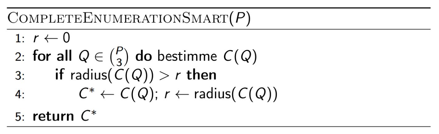
Korrektheit folgt aus den beiden Fakten: maximaler Radius unter allen \(Q\) liefert genau \(C(P)\).
Field-by-field Comparison
| Field |
Before |
After |
| Text |
|
<b>CompleteEnumerationSmart(\(P\)).</b><br>Statt für jedes \(Q\) die Bedingung \(P \subseteq C^{\bullet}(Q)\) zu prüfen, merkt man sich einfach {{c1::das \(Q\) mit dem grössten Radius \(\operatorname{radius}(C(Q))\)}}.<br><br>Laufzeit: {{c2::\(O(n^3)\)}}. |
| Extra |
|
<img src="paste-0b4588171e01f31b52efba2d64abcb883c72eb53.jpg"><br><br>Korrektheit folgt aus den beiden Fakten: maximaler Radius unter allen \(Q\) liefert genau \(C(P)\). |
Tags:
ETH::2._Semester::A&W::3._Algorithmen_-_Highlights::1._Graphenalgorithmen::4._Kleinster_umschliessender_Kreis::2._Erste_Algorithmen
Note 18: ETH::2. Semester::A&W
Deck: ETH::2. Semester::A&W
Note Type: Horvath Cloze
GUID: Ong0`FNR)`
added
Previous
Note did not exist
New Note
Front
ETH::2._Semester::A&W::3._Algorithmen_-_Highlights::1._Graphenalgorithmen::5._Konvexe_Hülle
Darstellung der konvexen Hülle (endliches \(P\) in der Ebene).
Der Rand von \(\operatorname{conv}(P)\) ist ein Polygon, dessen Ecken Punkte aus \(P\) sind. Die Berechnung von \(\operatorname{conv}(P)\) meint die Bestimmung der Eckenfolge \((q_0, q_1, \ldots, q_{h-1})\), \(h \leq n\), beginnend bei beliebigem \(q_0\) und gegen den Uhrzeigersinn entlang des Polygons.
Dabei ist \(Q := \{q_0, \ldots, q_{h-1}\}\) {{c4::die kleinste Teilmenge von \(P\) mit \(\operatorname{conv}(Q) = \operatorname{conv}(P)\)}}.
Back
ETH::2._Semester::A&W::3._Algorithmen_-_Highlights::1._Graphenalgorithmen::5._Konvexe_Hülle
Darstellung der konvexen Hülle (endliches \(P\) in der Ebene).
Der Rand von \(\operatorname{conv}(P)\) ist ein Polygon, dessen Ecken Punkte aus \(P\) sind. Die Berechnung von \(\operatorname{conv}(P)\) meint die Bestimmung der Eckenfolge \((q_0, q_1, \ldots, q_{h-1})\), \(h \leq n\), beginnend bei beliebigem \(q_0\) und gegen den Uhrzeigersinn entlang des Polygons.
Dabei ist \(Q := \{q_0, \ldots, q_{h-1}\}\) {{c4::die kleinste Teilmenge von \(P\) mit \(\operatorname{conv}(Q) = \operatorname{conv}(P)\)}}.
Field-by-field Comparison
| Field |
Before |
After |
| Text |
|
<b>Darstellung der konvexen Hülle (endliches \(P\) in der Ebene).</b><br>Der Rand von \(\operatorname{conv}(P)\) ist ein {{c1::Polygon}}, dessen Ecken {{c2::Punkte aus \(P\)}} sind. Die Berechnung von \(\operatorname{conv}(P)\) meint die Bestimmung der Eckenfolge \((q_0, q_1, \ldots, q_{h-1})\), \(h \leq n\), beginnend bei beliebigem \(q_0\) und {{c3::gegen den Uhrzeigersinn}} entlang des Polygons.<br><br>Dabei ist \(Q := \{q_0, \ldots, q_{h-1}\}\) {{c4::die kleinste Teilmenge von \(P\) mit \(\operatorname{conv}(Q) = \operatorname{conv}(P)\)}}. |
Tags:
ETH::2._Semester::A&W::3._Algorithmen_-_Highlights::1._Graphenalgorithmen::5._Konvexe_Hülle
Note 19: ETH::2. Semester::A&W
Deck: ETH::2. Semester::A&W
Note Type: Horvath Cloze
GUID: SLT}g*q+Wj
added
Previous
Note did not exist
New Note
Front
ETH::2._Semester::A&W::3._Algorithmen_-_Highlights::1._Graphenalgorithmen::5._Konvexe_Hülle
Anmerkungen zu LocalRepair.- Degeneriertheiten sind einfach einzubeziehen (lexikographisch sortieren, Duplikate danach entfernen, Test adaptieren).
- Numerisch robuster als JarvisWrap: kann nie in eine unendliche Schleife laufen.
- Liefert nebenbei eine Triangulierung der Punkte (lokale Verbesserung dient auch zur Berechnung guter, etwa Delaunay-, Triangulierungen).
- Optimal, aber: es gibt auch einen \(O(n \log h)\)-Algorithmus; für Punkte zufällig aus Quadrat/Kreisscheibe sogar erwartet \(O(n)\).
Back
ETH::2._Semester::A&W::3._Algorithmen_-_Highlights::1._Graphenalgorithmen::5._Konvexe_Hülle
Anmerkungen zu LocalRepair.- Degeneriertheiten sind einfach einzubeziehen (lexikographisch sortieren, Duplikate danach entfernen, Test adaptieren).
- Numerisch robuster als JarvisWrap: kann nie in eine unendliche Schleife laufen.
- Liefert nebenbei eine Triangulierung der Punkte (lokale Verbesserung dient auch zur Berechnung guter, etwa Delaunay-, Triangulierungen).
- Optimal, aber: es gibt auch einen \(O(n \log h)\)-Algorithmus; für Punkte zufällig aus Quadrat/Kreisscheibe sogar erwartet \(O(n)\).
Field-by-field Comparison
| Field |
Before |
After |
| Text |
|
<b>Anmerkungen zu LocalRepair.</b><br><ul><li>Degeneriertheiten sind einfach einzubeziehen (lexikographisch sortieren, Duplikate danach entfernen, Test adaptieren).</li><li>Numerisch {{c1::robuster als JarvisWrap}}: kann nie in eine unendliche Schleife laufen.</li><li>Liefert nebenbei {{c2::eine Triangulierung der Punkte}} (lokale Verbesserung dient auch zur Berechnung guter, etwa Delaunay-, Triangulierungen).</li><li>Optimal, aber: es gibt auch einen {{c3::\(O(n \log h)\)}}-Algorithmus; für Punkte zufällig aus Quadrat/Kreisscheibe sogar erwartet {{c4::\(O(n)\)}}.</li></ul> |
Tags:
ETH::2._Semester::A&W::3._Algorithmen_-_Highlights::1._Graphenalgorithmen::5._Konvexe_Hülle
Note 20: ETH::2. Semester::A&W
Deck: ETH::2. Semester::A&W
Note Type: Horvath Cloze
GUID: TW|Io^YoVH
added
Previous
Note did not exist
New Note
Front
ETH::2._Semester::A&W::3._Algorithmen_-_Highlights::1._Graphenalgorithmen::4._Kleinster_umschliessender_Kreis::2._Erste_Algorithmen
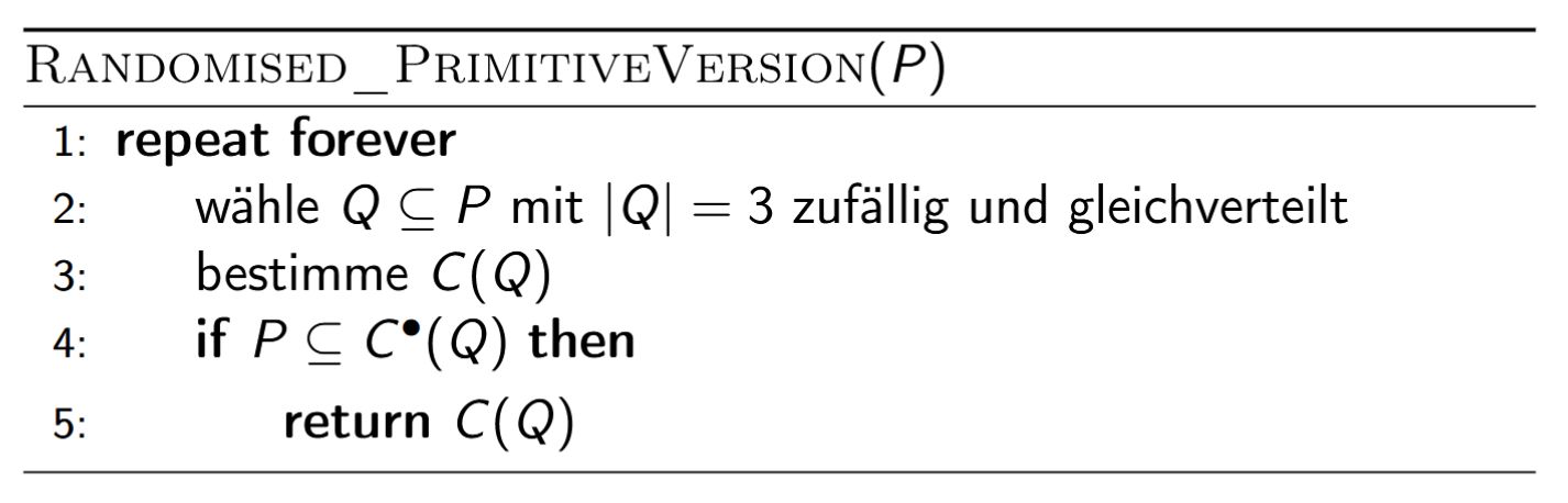
Man trifft das richtige \(Q\) mit Wahrscheinlichkeit {{c1::\(\geq 1 / \binom{n}{3}\)}}, die erwartete Anzahl Versuche ist also {{c2::\(\leq \binom{n}{3}\)}} und damit die erwartete Laufzeit
\(O(n^4)\).
Back
ETH::2._Semester::A&W::3._Algorithmen_-_Highlights::1._Graphenalgorithmen::4._Kleinster_umschliessender_Kreis::2._Erste_Algorithmen
Man trifft das richtige \(Q\) mit Wahrscheinlichkeit {{c1::\(\geq 1 / \binom{n}{3}\)}}, die erwartete Anzahl Versuche ist also {{c2::\(\leq \binom{n}{3}\)}} und damit die erwartete Laufzeit
\(O(n^4)\).
Idee zur Verbesserung: Man lernt, welche Punkte ausserhalb von \(C(Q)\) liegen: diese sind wichtiger für \(C(P)\) als die Punkte innerhalb.
Field-by-field Comparison
| Field |
Before |
After |
| Text |
|
<img src="paste-cc7618eee9d33a5618aa3d281ebffa88757498e6.jpg"><br><br>Man trifft das richtige \(Q\) mit Wahrscheinlichkeit {{c1::\(\geq 1 / \binom{n}{3}\)}}, die erwartete Anzahl Versuche ist also {{c2::\(\leq \binom{n}{3}\)}} und damit die erwartete Laufzeit {{c3::\(O(n^4)\)}}. |
| Extra |
|
Idee zur Verbesserung: Man lernt, welche Punkte ausserhalb von \(C(Q)\) liegen: diese sind wichtiger für \(C(P)\) als die Punkte innerhalb. |
Tags:
ETH::2._Semester::A&W::3._Algorithmen_-_Highlights::1._Graphenalgorithmen::4._Kleinster_umschliessender_Kreis::2._Erste_Algorithmen
Note 21: ETH::2. Semester::A&W
Deck: ETH::2. Semester::A&W
Note Type: Horvath Classic
GUID: T{c0*2V>r{
added
Previous
Note did not exist
New Note
Front
ETH::2._Semester::A&W::3._Algorithmen_-_Highlights::1._Graphenalgorithmen::5._Konvexe_Hülle
Invarianten während der lokalen Verbesserungen (LocalRepair).
Welche drei Invarianten gelten für den Hin-Zug \((p_1, \ldots, p_n)\) und den Rück-Zug \((p_n, \ldots, p_1)\)?
Back
ETH::2._Semester::A&W::3._Algorithmen_-_Highlights::1._Graphenalgorithmen::5._Konvexe_Hülle
Invarianten während der lokalen Verbesserungen (LocalRepair).
Welche drei Invarianten gelten für den Hin-Zug \((p_1, \ldots, p_n)\) und den Rück-Zug \((p_n, \ldots, p_1)\)?
- \((p_1, \ldots, p_n)\) ist \(x\)-monoton (links nach rechts) und hat keinen Punkt aus \(P\) unter sich.
- \((p_n, \ldots, p_1)\) ist \(x\)-monoton (rechts nach links) und hat keinen Punkt aus \(P\) unter sich.
- \((p_1, \ldots, p_n)\) liegt nirgends über \((p_n, \ldots, p_1)\).
Folge: Das Polygon kann sich nie selbst kreuzen und umschliesst alle Punkte, also gilt: lokal konvex \(\Rightarrow\) Lösungspolygon.
Field-by-field Comparison
| Field |
Before |
After |
| Front |
|
<b>Invarianten während der lokalen Verbesserungen (LocalRepair).</b><br>Welche drei Invarianten gelten für den Hin-Zug \((p_1, \ldots, p_n)\) und den Rück-Zug \((p_n, \ldots, p_1)\)? |
| Back |
|
<ul><li>\((p_1, \ldots, p_n)\) ist \(x\)-monoton (links nach rechts) und hat keinen Punkt aus \(P\) unter sich.</li><li>\((p_n, \ldots, p_1)\) ist \(x\)-monoton (rechts nach links) und hat keinen Punkt aus \(P\) unter sich.</li><li>\((p_1, \ldots, p_n)\) liegt nirgends über \((p_n, \ldots, p_1)\).</li></ul>Folge: Das Polygon kann sich nie selbst kreuzen und umschliesst alle Punkte, also gilt: lokal konvex \(\Rightarrow\) Lösungspolygon. |
Tags:
ETH::2._Semester::A&W::3._Algorithmen_-_Highlights::1._Graphenalgorithmen::5._Konvexe_Hülle
Note 22: ETH::2. Semester::A&W
Deck: ETH::2. Semester::A&W
Note Type: Horvath Cloze
GUID: T}}KX)AY2w
added
Previous
Note did not exist
New Note
Front
ETH::2._Semester::A&W::3._Algorithmen_-_Highlights::1._Graphenalgorithmen::5._Konvexe_Hülle
Vereinfachende Annahme: Allgemeine Lage.
Für die ConvexHull-Algorithmen nimmt man an, dass keine 3 Punkte auf einer gemeinsamen Geraden liegen und keine 2 Punkte dieselbe \(x\)-Koordinate haben.
Back
ETH::2._Semester::A&W::3._Algorithmen_-_Highlights::1._Graphenalgorithmen::5._Konvexe_Hülle
Vereinfachende Annahme: Allgemeine Lage.
Für die ConvexHull-Algorithmen nimmt man an, dass keine 3 Punkte auf einer gemeinsamen Geraden liegen und keine 2 Punkte dieselbe \(x\)-Koordinate haben.
Diese Annahme schliesst Kollinearitäten und Mehrdeutigkeiten aus: Degeneriertheiten werden separat behandelt.
Field-by-field Comparison
| Field |
Before |
After |
| Text |
|
<b>Vereinfachende Annahme: Allgemeine Lage.</b><br>Für die ConvexHull-Algorithmen nimmt man an, dass {{c1::keine 3 Punkte auf einer gemeinsamen Geraden liegen}} und {{c2::keine 2 Punkte dieselbe \(x\)-Koordinate haben}}. |
| Extra |
|
Diese Annahme schliesst Kollinearitäten und Mehrdeutigkeiten aus: Degeneriertheiten werden separat behandelt. |
Tags:
ETH::2._Semester::A&W::3._Algorithmen_-_Highlights::1._Graphenalgorithmen::5._Konvexe_Hülle
Note 23: ETH::2. Semester::A&W
Deck: ETH::2. Semester::A&W
Note Type: Horvath Cloze
GUID: VqE4Q6Sl#s
added
Previous
Note did not exist
New Note
Front
ETH::2._Semester::A&W::3._Algorithmen_-_Highlights::1._Graphenalgorithmen::4._Kleinster_umschliessender_Kreis::1._Grundlagen
Kleine bestimmende Menge
Für jede Punktemenge \(P \subseteq \mathbb{R}^2\) mit \(|P| \geq 3\) gibt es eine Teilmenge \(Q \subseteq P\) mit \(|Q| = 3\) und \(C(Q) = C(P)\).
Ein solches \(Q\) heisst Zertifikat für \(C(P)\).
Back
ETH::2._Semester::A&W::3._Algorithmen_-_Highlights::1._Graphenalgorithmen::4._Kleinster_umschliessender_Kreis::1._Grundlagen
Kleine bestimmende Menge
Für jede Punktemenge \(P \subseteq \mathbb{R}^2\) mit \(|P| \geq 3\) gibt es eine Teilmenge \(Q \subseteq P\) mit \(|Q| = 3\) und \(C(Q) = C(P)\).
Ein solches \(Q\) heisst Zertifikat für \(C(P)\).
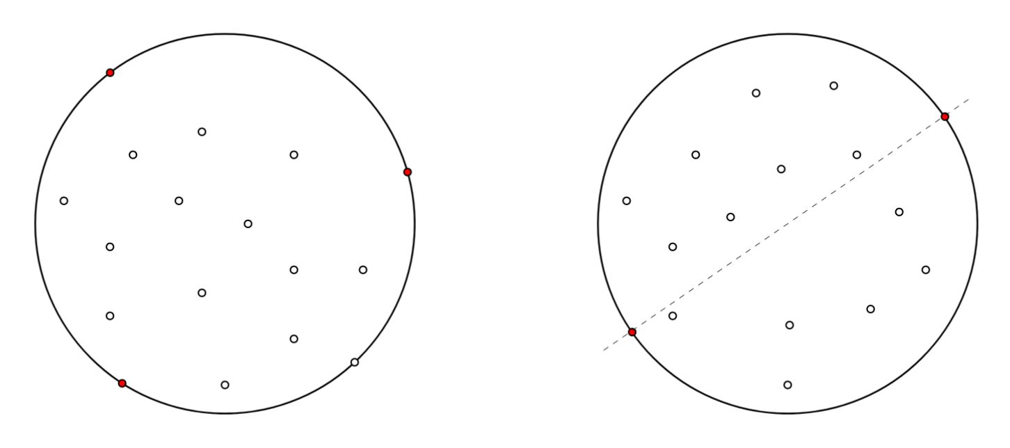
Hier ohne Beweis (siehe Skript).
Field-by-field Comparison
| Field |
Before |
After |
| Text |
|
<b>Kleine bestimmende Menge</b><br>Für jede Punktemenge \(P \subseteq \mathbb{R}^2\) mit \(|P| \geq 3\) gibt es eine Teilmenge \(Q \subseteq P\) mit {{c1::\(|Q| = 3\)}} und {{c2::\(C(Q) = C(P)\)}}.<br><br>Ein solches \(Q\) heisst {{c3::Zertifikat für \(C(P)\)}}. |
| Extra |
|
<img src="paste-c802629281d2c7732b885cb14f4ca8c51ff57875.jpg"><br><br>Hier ohne Beweis (siehe Skript). |
Tags:
ETH::2._Semester::A&W::3._Algorithmen_-_Highlights::1._Graphenalgorithmen::4._Kleinster_umschliessender_Kreis::1._Grundlagen
Note 24: ETH::2. Semester::A&W
Deck: ETH::2. Semester::A&W
Note Type: Horvath Classic
GUID: WYr#p/)og,
added
Previous
Note did not exist
New Note
Front
ETH::2._Semester::A&W::3._Algorithmen_-_Highlights::1._Graphenalgorithmen::5._Konvexe_Hülle
Satz + Optimalität von LocalRepair.
Was besagt der Laufzeit-Satz für bereits \(x\)-sortierte Punkte, und warum ist der Algorithmus optimal?
Back
ETH::2._Semester::A&W::3._Algorithmen_-_Highlights::1._Graphenalgorithmen::5._Konvexe_Hülle
Satz + Optimalität von LocalRepair.
Was besagt der Laufzeit-Satz für bereits \(x\)-sortierte Punkte, und warum ist der Algorithmus optimal?
Für nach \(x\)-Koordinate sortierte Punkte in allgemeiner Lage berechnet LocalRepair die konvexe Hülle von \(\{p_1, \ldots, p_n\}\) in Zeit \(O(n)\).
Da Sortieren (\(\Omega(n \log n)\)) auf ConvexHull reduzierbar ist, ist LocalRepair (inkl. Sortieren) optimal.
Field-by-field Comparison
| Field |
Before |
After |
| Front |
|
<b>Satz + Optimalität von LocalRepair.</b><br>Was besagt der Laufzeit-Satz für bereits \(x\)-sortierte Punkte, und warum ist der Algorithmus optimal? |
| Back |
|
Für nach \(x\)-Koordinate sortierte Punkte in allgemeiner Lage berechnet LocalRepair die konvexe Hülle von \(\{p_1, \ldots, p_n\}\) in Zeit \(O(n)\).<br><br>Da Sortieren (\(\Omega(n \log n)\)) auf ConvexHull reduzierbar ist, ist LocalRepair (inkl. Sortieren) <b>optimal</b>. |
Tags:
ETH::2._Semester::A&W::3._Algorithmen_-_Highlights::1._Graphenalgorithmen::5._Konvexe_Hülle
Note 25: ETH::2. Semester::A&W
Deck: ETH::2. Semester::A&W
Note Type: Horvath Cloze
GUID: XGaR5ZRd8Z
added
Previous
Note did not exist
New Note
Front
ETH::2._Semester::A&W::3._Algorithmen_-_Highlights::1._Graphenalgorithmen::5._Konvexe_Hülle
Konsequenz der Invarianten + Nichtdeterminismus.
Dank der drei Invarianten gilt: lokal konvex \(\Rightarrow\) Lösungspolygon (kein Selbstschnitt, alle Punkte umschlossen).
Ausserdem ist der Algorithmus zunächst nicht-deterministisch: die lokalen Verbesserungsschritte dürfen in beliebiger Reihenfolge ausgeführt werden.
Back
ETH::2._Semester::A&W::3._Algorithmen_-_Highlights::1._Graphenalgorithmen::5._Konvexe_Hülle
Konsequenz der Invarianten + Nichtdeterminismus.
Dank der drei Invarianten gilt: lokal konvex \(\Rightarrow\) Lösungspolygon (kein Selbstschnitt, alle Punkte umschlossen).
Ausserdem ist der Algorithmus zunächst nicht-deterministisch: die lokalen Verbesserungsschritte dürfen in beliebiger Reihenfolge ausgeführt werden.
Field-by-field Comparison
| Field |
Before |
After |
| Text |
|
<b>Konsequenz der Invarianten + Nichtdeterminismus.</b><br>Dank der drei Invarianten gilt: {{c1::lokal konvex \(\Rightarrow\) Lösungspolygon}} (kein Selbstschnitt, alle Punkte umschlossen).<br><br>Ausserdem ist der Algorithmus zunächst {{c2::nicht-deterministisch}}: die lokalen Verbesserungsschritte dürfen in {{c2::beliebiger Reihenfolge}} ausgeführt werden. |
Tags:
ETH::2._Semester::A&W::3._Algorithmen_-_Highlights::1._Graphenalgorithmen::5._Konvexe_Hülle
Note 26: ETH::2. Semester::A&W
Deck: ETH::2. Semester::A&W
Note Type: Horvath Classic
GUID: YdaR[CTQLC
added
Previous
Note did not exist
New Note
Front
ETH::2._Semester::A&W::3._Algorithmen_-_Highlights::1._Graphenalgorithmen::5._Konvexe_Hülle
Lemma (Ordnung um eine Hüllen-Ecke).
Sei \(q\) eine Ecke der konvexen Hülle von \(P\). Was gilt für die Relation \(\prec_q\) auf \(P \setminus \{q\}\), und was bedeutet ihr Minimum?
Back
ETH::2._Semester::A&W::3._Algorithmen_-_Highlights::1._Graphenalgorithmen::5._Konvexe_Hülle
Lemma (Ordnung um eine Hüllen-Ecke).
Sei \(q\) eine Ecke der konvexen Hülle von \(P\). Was gilt für die Relation \(\prec_q\) auf \(P \setminus \{q\}\), und was bedeutet ihr Minimum?
\(\prec_q\) ist eine totale Ordnung auf \(P \setminus \{q\}\). Für das Minimum \(p_{\min}\) dieser Ordnung gilt: \(q, p_{\min}\) ist eine Randkante.
Damit liefert ein einzelner Min-Durchlauf (wie in FindNext) die nächste Hüllenkante.
Field-by-field Comparison
| Field |
Before |
After |
| Front |
|
<b>Lemma (Ordnung um eine Hüllen-Ecke).</b><br>Sei \(q\) eine Ecke der konvexen Hülle von \(P\). Was gilt für die Relation \(\prec_q\) auf \(P \setminus \{q\}\), und was bedeutet ihr Minimum? |
| Back |
|
\(\prec_q\) ist eine <b>totale Ordnung</b> auf \(P \setminus \{q\}\). Für das Minimum \(p_{\min}\) dieser Ordnung gilt: \(q, p_{\min}\) ist eine <b>Randkante</b>.<br><br>Damit liefert ein einzelner Min-Durchlauf (wie in <code>FindNext</code>) die nächste Hüllenkante. |
Tags:
ETH::2._Semester::A&W::3._Algorithmen_-_Highlights::1._Graphenalgorithmen::5._Konvexe_Hülle
Note 27: ETH::2. Semester::A&W
Deck: ETH::2. Semester::A&W
Note Type: Horvath Cloze
GUID: [,E,9zW4{2
added
Previous
Note did not exist
New Note
Front
ETH::2._Semester::A&W::3._Algorithmen_-_Highlights::1._Graphenalgorithmen::5._Konvexe_Hülle
JarvisWrap: numerische Probleme.
Der Orientierungsausdruck \((r_x - q_x)(p_y - q_y) - (p_x - q_x)(r_y - q_y) > 0\) ist mit Fliesskommazahlen nicht exakt. Kritisch ist dabei oft nicht die absolute Genauigkeit, sondern dass der Algorithmus völlig falsche Ergebnisse liefern oder in eine unendliche Schleife laufen kann (z.B. Vorbeilaufen am Startpunkt, weil dieser doppelt auftritt).
Abhilfe: Programmbibliotheken mit exakten Datentypen (für spezielle Operationen).
Back
ETH::2._Semester::A&W::3._Algorithmen_-_Highlights::1._Graphenalgorithmen::5._Konvexe_Hülle
JarvisWrap: numerische Probleme.
Der Orientierungsausdruck \((r_x - q_x)(p_y - q_y) - (p_x - q_x)(r_y - q_y) > 0\) ist mit Fliesskommazahlen nicht exakt. Kritisch ist dabei oft nicht die absolute Genauigkeit, sondern dass der Algorithmus völlig falsche Ergebnisse liefern oder in eine unendliche Schleife laufen kann (z.B. Vorbeilaufen am Startpunkt, weil dieser doppelt auftritt).
Abhilfe: Programmbibliotheken mit exakten Datentypen (für spezielle Operationen).
Field-by-field Comparison
| Field |
Before |
After |
| Text |
|
<b>JarvisWrap: numerische Probleme.</b><br>Der Orientierungsausdruck \((r_x - q_x)(p_y - q_y) - (p_x - q_x)(r_y - q_y) > 0\) ist mit Fliesskommazahlen nicht exakt. Kritisch ist dabei oft nicht die absolute Genauigkeit, sondern dass der Algorithmus {{c1::völlig falsche Ergebnisse liefern oder in eine unendliche Schleife laufen}} kann (z.B. {{c2::Vorbeilaufen am Startpunkt}}, weil dieser doppelt auftritt).<br><br>Abhilfe: {{c3::Programmbibliotheken mit exakten Datentypen}} (für spezielle Operationen). |
Tags:
ETH::2._Semester::A&W::3._Algorithmen_-_Highlights::1._Graphenalgorithmen::5._Konvexe_Hülle
Note 28: ETH::2. Semester::A&W
Deck: ETH::2. Semester::A&W
Note Type: Horvath Classic
GUID: [/jcw,k!?v
added
Previous
Note did not exist
New Note
Front
ETH::2._Semester::A&W::3._Algorithmen_-_Highlights::1._Graphenalgorithmen::5._Konvexe_Hülle
Lemma (Randkanten charakterisieren die Hülle).
Wann ist \((q_0, q_1, \ldots, q_{h-1})\) die Eckenfolge des \(\operatorname{conv}(P)\) umschliessenden Polygons gegen den Uhrzeigersinn? (Indizes \(\bmod\, h\))
Back
ETH::2._Semester::A&W::3._Algorithmen_-_Highlights::1._Graphenalgorithmen::5._Konvexe_Hülle
Lemma (Randkanten charakterisieren die Hülle).
Wann ist \((q_0, q_1, \ldots, q_{h-1})\) die Eckenfolge des \(\operatorname{conv}(P)\) umschliessenden Polygons gegen den Uhrzeigersinn? (Indizes \(\bmod\, h\))
Genau dann, wenn alle Paare \((q_{i-1}, q_i)\), \(i = 1, 2, \ldots, h\), Randkanten von \(P\) sind (Indizes \(\bmod\, h\)).
Das übersetzt die globale Eigenschaft "Eckenfolge der Hülle" in lokal prüfbare Randkanten-Bedingungen.
Field-by-field Comparison
| Field |
Before |
After |
| Front |
|
<b>Lemma (Randkanten charakterisieren die Hülle).</b><br>Wann ist \((q_0, q_1, \ldots, q_{h-1})\) die Eckenfolge des \(\operatorname{conv}(P)\) umschliessenden Polygons gegen den Uhrzeigersinn? (Indizes \(\bmod\, h\)) |
| Back |
|
<b>Genau dann, wenn</b> alle Paare \((q_{i-1}, q_i)\), \(i = 1, 2, \ldots, h\), <b>Randkanten von \(P\)</b> sind (Indizes \(\bmod\, h\)).<br><br>Das übersetzt die globale Eigenschaft "Eckenfolge der Hülle" in lokal prüfbare Randkanten-Bedingungen. |
Tags:
ETH::2._Semester::A&W::3._Algorithmen_-_Highlights::1._Graphenalgorithmen::5._Konvexe_Hülle
Note 29: ETH::2. Semester::A&W
Deck: ETH::2. Semester::A&W
Note Type: Horvath Classic
GUID: ^nab<])F=$
added
Previous
Note did not exist
New Note
Front
ETH::2._Semester::A&W::3._Algorithmen_-_Highlights::1._Graphenalgorithmen::5._Konvexe_Hülle
Untere Schranke für ConvexHull (Reduktion von Sortieren).
Wie projiziert man eine Zahlenfolge \((x_1, \ldots, x_n)\), um Sortieren auf ConvexHull zu reduzieren, und welche Schranke folgt?
Back
ETH::2._Semester::A&W::3._Algorithmen_-_Highlights::1._Graphenalgorithmen::5._Konvexe_Hülle
Untere Schranke für ConvexHull (Reduktion von Sortieren).
Wie projiziert man eine Zahlenfolge \((x_1, \ldots, x_n)\), um Sortieren auf ConvexHull zu reduzieren, und welche Schranke folgt?
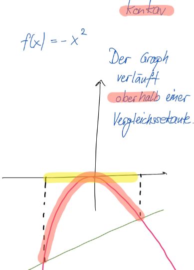
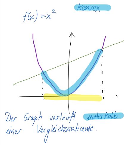
Setze \(p_i = (x_i, x_i^2)\), also vertikale Projektion auf die Parabel \(y = x^2\). Aus der Eckenfolge der konvexen Hülle von \(P = \{p_1, \ldots, p_n\}\) liest man in linearer Zeit die aufsteigend sortierte Reihenfolge der \(x_i\) ab.
Reduktion: Kann man ConvexHull in \(t(n)\) lösen, so kann man in \(t(n) + O(n)\) sortieren. Damit ist \(\Omega(n \log n)\) eine untere Schranke für ConvexHull.
Field-by-field Comparison
| Field |
Before |
After |
| Front |
|
<b>Untere Schranke für ConvexHull (Reduktion von Sortieren).</b><br>Wie projiziert man eine Zahlenfolge \((x_1, \ldots, x_n)\), um Sortieren auf ConvexHull zu reduzieren, und welche Schranke folgt? |
| Back |
|
Setze \(p_i = (x_i, x_i^2)\), also vertikale Projektion auf die Parabel \(y = x^2\). Aus der Eckenfolge der konvexen Hülle von \(P = \{p_1, \ldots, p_n\}\) liest man in linearer Zeit die aufsteigend sortierte Reihenfolge der \(x_i\) ab.<br><br><b>Reduktion:</b> Kann man ConvexHull in \(t(n)\) lösen, so kann man in \(t(n) + O(n)\) sortieren. Damit ist \(\Omega(n \log n)\) eine untere Schranke für ConvexHull. |
Tags:
ETH::2._Semester::A&W::3._Algorithmen_-_Highlights::1._Graphenalgorithmen::5._Konvexe_Hülle
Note 30: ETH::2. Semester::A&W
Deck: ETH::2. Semester::A&W
Note Type: Horvath Cloze
GUID: `/B}()b0J3
added
Previous
Note did not exist
New Note
Front
ETH::2._Semester::A&W::3._Algorithmen_-_Highlights::1._Graphenalgorithmen::5._Konvexe_Hülle
Orientierungstest (links/rechts).
Die vorzeichenbehaftete Fläche des von \(o = (0,0)\), \(r\) und \(p\) aufgespannten Parallelogramms ist \(\det(r, p) = r_x p_y - p_x r_y\).
\(p\) liegt links von \(o, r\) \(\iff r_x p_y - p_x r_y > 0\).
Back
ETH::2._Semester::A&W::3._Algorithmen_-_Highlights::1._Graphenalgorithmen::5._Konvexe_Hülle
Orientierungstest (links/rechts).
Die vorzeichenbehaftete Fläche des von \(o = (0,0)\), \(r\) und \(p\) aufgespannten Parallelogramms ist \(\det(r, p) = r_x p_y - p_x r_y\).
\(p\) liegt links von \(o, r\) \(\iff r_x p_y - p_x r_y > 0\).
Hintergrund: \(\det(r,p) = \|r\|\,\|p\|\sin\angle(r,o,p)\); das Vorzeichen des Sinus codiert die Drehrichtung (\(>0\) für \(0^\circ < \alpha < 180^\circ\)).
Field-by-field Comparison
| Field |
Before |
After |
| Text |
|
<b>Orientierungstest (links/rechts).</b><br>Die vorzeichenbehaftete Fläche des von \(o = (0,0)\), \(r\) und \(p\) aufgespannten Parallelogramms ist \(\det(r, p) = {{c1::r_x p_y - p_x r_y}}\).<br><br>\(p\) liegt <b>links</b> von \(o, r\) \(\iff {{c2::r_x p_y - p_x r_y > 0}}\). |
| Extra |
|
Hintergrund: \(\det(r,p) = \|r\|\,\|p\|\sin\angle(r,o,p)\); das Vorzeichen des Sinus codiert die Drehrichtung (\(>0\) für \(0^\circ < \alpha < 180^\circ\)). |
Tags:
ETH::2._Semester::A&W::3._Algorithmen_-_Highlights::1._Graphenalgorithmen::5._Konvexe_Hülle
Note 31: ETH::2. Semester::A&W
Deck: ETH::2. Semester::A&W
Note Type: Horvath Cloze
GUID: a2~{ya,S_m
modified
Before
Front
ETH::2._Semester::A&W::3._Algorithmen_-_Highlights::1._Graphenalgorithmen::3._Minimale_Schnitte_in_Graphen
Satz. Wiederholt man \(\textsc{Cut}(G)\) \(\alpha \binom{n}{2}\)-mal und gibt den kleinsten erhaltenen Wert aus, so gilt:
- Laufzeit \({{c1::\mathcal{O}(\alpha n^4)}}\).
- Der ausgegebene Wert ist mit Wahrscheinlichkeit mindestens \(1 - e^{-\alpha}\) gleich \(\mu(G)\).
Back
ETH::2._Semester::A&W::3._Algorithmen_-_Highlights::1._Graphenalgorithmen::3._Minimale_Schnitte_in_Graphen
Satz. Wiederholt man \(\textsc{Cut}(G)\) \(\alpha \binom{n}{2}\)-mal und gibt den kleinsten erhaltenen Wert aus, so gilt:
- Laufzeit \({{c1::\mathcal{O}(\alpha n^4)}}\).
- Der ausgegebene Wert ist mit Wahrscheinlichkeit mindestens \(1 - e^{-\alpha}\) gleich \(\mu(G)\).
Begründung Erfolgswahrscheinlichkeit: jede Einzelausführung scheitert mit Wkt. \(\leq 1 - 1/\binom{n}{2}\). Bei \(\alpha\binom{n}{2}\) unabhängigen Wiederholungen ist die Misserfolgswkt. höchstens \((1 - 1/\binom{n}{2})^{\alpha\binom{n}{2}} \leq e^{-\alpha}\).
Mit \(\alpha := \ln n\) erhält man Zeit \(\mathcal{O}(n^4 \log n)\) bei Fehlerwkt. \(\leq 1/n\); aber diese Laufzeit hatten wir bereits deterministisch.
After
Front
ETH::2._Semester::A&W::3._Algorithmen_-_Highlights::1._Graphenalgorithmen::3._Minimale_Schnitte_in_Graphen
Wiederholt man \(\text{Cut}(G)\) \(\alpha \binom{n}{2}\)-mal und gibt den kleinsten erhaltenen Wert aus, so gilt:
- Laufzeit \({{c1::\mathcal{O}(\alpha n^4)}}\).
- Der ausgegebene Wert ist mit Wahrscheinlichkeit mindestens \({{c2::1 - e^{-\alpha} }}\) gleich \(\mu(G)\).
Back
ETH::2._Semester::A&W::3._Algorithmen_-_Highlights::1._Graphenalgorithmen::3._Minimale_Schnitte_in_Graphen
Wiederholt man \(\text{Cut}(G)\) \(\alpha \binom{n}{2}\)-mal und gibt den kleinsten erhaltenen Wert aus, so gilt:
- Laufzeit \({{c1::\mathcal{O}(\alpha n^4)}}\).
- Der ausgegebene Wert ist mit Wahrscheinlichkeit mindestens \({{c2::1 - e^{-\alpha} }}\) gleich \(\mu(G)\).
Begründung Erfolgswahrscheinlichkeit: jede Einzelausführung scheitert mit Wkt. \(\leq 1 - 1/\binom{n}{2}\). Bei \(\alpha\binom{n}{2}\) unabhängigen Wiederholungen ist die Misserfolgswkt. höchstens \((1 - 1/\binom{n}{2})^{\alpha\binom{n}{2}} \leq e^{-\alpha}\).
Mit \(\alpha := \ln n\) erhält man Zeit \(\mathcal{O}(n^4 \log n)\) bei Fehlerwkt. \(\leq 1/n\); aber diese Laufzeit hatten wir bereits deterministisch.
Field-by-field Comparison
| Field |
Before |
After |
| Text |
<b>Satz.</b> Wiederholt man \(\textsc{Cut}(G)\) \(\alpha \binom{n}{2}\)-mal und gibt den kleinsten erhaltenen Wert aus, so gilt:<ol><li>Laufzeit \({{c1::\mathcal{O}(\alpha n^4)}}\).</li><li>Der ausgegebene Wert ist mit Wahrscheinlichkeit mindestens \({{c2::1 - e^{-\alpha}}}\) gleich \(\mu(G)\).</li></ol> |
Wiederholt man \(\text{Cut}(G)\) \(\alpha \binom{n}{2}\)-mal und gibt den kleinsten erhaltenen Wert aus, so gilt:<ol><li>Laufzeit \({{c1::\mathcal{O}(\alpha n^4)}}\).</li><li>Der ausgegebene Wert ist mit Wahrscheinlichkeit mindestens \({{c2::1 - e^{-\alpha} }}\) gleich \(\mu(G)\).</li></ol> |
Tags:
ETH::2._Semester::A&W::3._Algorithmen_-_Highlights::1._Graphenalgorithmen::3._Minimale_Schnitte_in_Graphen
Note 32: ETH::2. Semester::A&W
Deck: ETH::2. Semester::A&W
Note Type: Horvath Cloze
GUID: apk?tD
added
Previous
Note did not exist
New Note
Front
ETH::2._Semester::A&W::3._Algorithmen_-_Highlights::1._Graphenalgorithmen::4._Kleinster_umschliessender_Kreis::4._Sampling_Lemma
Sampling Lemma.
Seien \(r, N \in \mathbb{N}\), \(r \leq N\), und \(P'\) eine Multimenge mit \(|P'| = N\).
Für \(R\) zufällig gleichverteilt aus \(\binom{P'}{r}\) gilt\[\mathbb{E}\big[\,|P' \setminus C^{\bullet}(R)|\,\big] \;\leq\; {{c1::3\,\frac{N - r}{r + 1} }} \;\leq\; {{c1::3\,\frac{N}{r + 1} }}.\]
Back
ETH::2._Semester::A&W::3._Algorithmen_-_Highlights::1._Graphenalgorithmen::4._Kleinster_umschliessender_Kreis::4._Sampling_Lemma
Sampling Lemma.
Seien \(r, N \in \mathbb{N}\), \(r \leq N\), und \(P'\) eine Multimenge mit \(|P'| = N\).
Für \(R\) zufällig gleichverteilt aus \(\binom{P'}{r}\) gilt\[\mathbb{E}\big[\,|P' \setminus C^{\bullet}(R)|\,\big] \;\leq\; {{c1::3\,\frac{N - r}{r + 1} }} \;\leq\; {{c1::3\,\frac{N}{r + 1} }}.\]
\(|P' \setminus C^{\bullet}(R)|\) ist die Anzahl der Punkte aus \(P'\), die ausserhalb von \(C(R)\) liegen. Diese Schranke kontrolliert das Wachstum von \(P'\) pro Runde.
Field-by-field Comparison
| Field |
Before |
After |
| Text |
|
<b>Sampling Lemma.</b><br>Seien \(r, N \in \mathbb{N}\), \(r \leq N\), und \(P'\) eine Multimenge mit \(|P'| = N\). <br>Für \(R\) zufällig gleichverteilt aus \(\binom{P'}{r}\) gilt\[\mathbb{E}\big[\,|P' \setminus C^{\bullet}(R)|\,\big] \;\leq\; {{c1::3\,\frac{N - r}{r + 1} }} \;\leq\; {{c1::3\,\frac{N}{r + 1} }}.\] |
| Extra |
|
\(|P' \setminus C^{\bullet}(R)|\) ist die Anzahl der Punkte aus \(P'\), die ausserhalb von \(C(R)\) liegen. Diese Schranke kontrolliert das Wachstum von \(P'\) pro Runde. |
Tags:
ETH::2._Semester::A&W::3._Algorithmen_-_Highlights::1._Graphenalgorithmen::4._Kleinster_umschliessender_Kreis::4._Sampling_Lemma
Note 33: ETH::2. Semester::A&W
Deck: ETH::2. Semester::A&W
Note Type: Horvath Cloze
GUID: bX&z[6rdCT
added
Previous
Note did not exist
New Note
Front
ETH::2._Semester::A&W::3._Algorithmen_-_Highlights::1._Graphenalgorithmen::5._Konvexe_Hülle
Jarvis Wrap (Einwickeln).Startend bei \(q_0\) (kleinste \(x\)-Koordinate) hängt man wiederholt {{c1::\(q_h \leftarrow \texttt{FindNext}(q_{h-1})\)}} an, bis
\(q_h = q_0\) (die Hülle ist geschlossen):
JarvisWrap(P):
  q₀ ← Punkt in P mit kleinster x-Koordinate
  h ← 0
  repeat:
    h ← h + 1
    q_h ← FindNext(q_{h-1})
  until q_h = q₀
  return (q₀, q₁, ..., q_{h-1})
Back
ETH::2._Semester::A&W::3._Algorithmen_-_Highlights::1._Graphenalgorithmen::5._Konvexe_Hülle
Jarvis Wrap (Einwickeln).Startend bei \(q_0\) (kleinste \(x\)-Koordinate) hängt man wiederholt {{c1::\(q_h \leftarrow \texttt{FindNext}(q_{h-1})\)}} an, bis
\(q_h = q_0\) (die Hülle ist geschlossen):
JarvisWrap(P):
  q₀ ← Punkt in P mit kleinster x-Koordinate
  h ← 0
  repeat:
    h ← h + 1
    q_h ← FindNext(q_{h-1})
  until q_h = q₀
  return (q₀, q₁, ..., q_{h-1})
Field-by-field Comparison
| Field |
Before |
After |
| Text |
|
<b>Jarvis Wrap (Einwickeln).</b><br>Startend bei \(q_0\) (kleinste \(x\)-Koordinate) hängt man wiederholt {{c1::\(q_h \leftarrow \texttt{FindNext}(q_{h-1})\)}} an, bis {{c2::\(q_h = q_0\)}} (die Hülle ist geschlossen):<pre>JarvisWrap(P):
q₀ ← Punkt in P mit kleinster x-Koordinate
h ← 0
repeat:
h ← h + 1
q_h ← FindNext(q_{h-1})
until q_h = q₀
return (q₀, q₁, ..., q_{h-1})</pre> |
Tags:
ETH::2._Semester::A&W::3._Algorithmen_-_Highlights::1._Graphenalgorithmen::5._Konvexe_Hülle
Note 34: ETH::2. Semester::A&W
Deck: ETH::2. Semester::A&W
Note Type: Horvath Cloze
GUID: c5nKNDt/nl
added
Previous
Note did not exist
New Note
Front
ETH::2._Semester::A&W::3._Algorithmen_-_Highlights::1._Graphenalgorithmen::4._Kleinster_umschliessender_Kreis::1._Grundlagen
Für jede endliche Punktemenge \(P \subseteq \mathbb{R}^2\) gibt es einen eindeutigen kleinsten umschliessenden Kreis \(C(P)\).
Back
ETH::2._Semester::A&W::3._Algorithmen_-_Highlights::1._Graphenalgorithmen::4._Kleinster_umschliessender_Kreis::1._Grundlagen
Für jede endliche Punktemenge \(P \subseteq \mathbb{R}^2\) gibt es einen eindeutigen kleinsten umschliessenden Kreis \(C(P)\).
Field-by-field Comparison
| Field |
Before |
After |
| Text |
|
Für jede endliche Punktemenge \(P \subseteq \mathbb{R}^2\) gibt es einen {{c1::eindeutigen kleinsten umschliessenden Kreis \(C(P)\)}}. |
| Extra |
|
<img src="paste-40de2930df9c9fff72e022c067c852e3b4fe033f.jpg"> |
Tags:
ETH::2._Semester::A&W::3._Algorithmen_-_Highlights::1._Graphenalgorithmen::4._Kleinster_umschliessender_Kreis::1._Grundlagen
Note 35: ETH::2. Semester::A&W
Deck: ETH::2. Semester::A&W
Note Type: Horvath Cloze
GUID: czl;f!y3J*
added
Previous
Note did not exist
New Note
Front
ETH::2._Semester::A&W::3._Algorithmen_-_Highlights::1._Graphenalgorithmen::5._Konvexe_Hülle
Liniensegment und Konvexität.
Für \(v_0, v_1 \in \mathbb{R}^d\) ist das verbindende Liniensegment \(\overline{v_0 v_1} := {{c1::\{(1-\lambda)v_0 + \lambda v_1 \mid \lambda \in \mathbb{R},\ 0 \leq \lambda \leq 1\} }}\).
Eine Menge \(C \subseteq \mathbb{R}^d\) heisst konvex, falls {{c2::\(\forall v_0, v_1 \in C: \overline{v_0 v_1} \subseteq C\)}}.
Back
ETH::2._Semester::A&W::3._Algorithmen_-_Highlights::1._Graphenalgorithmen::5._Konvexe_Hülle
Liniensegment und Konvexität.
Für \(v_0, v_1 \in \mathbb{R}^d\) ist das verbindende Liniensegment \(\overline{v_0 v_1} := {{c1::\{(1-\lambda)v_0 + \lambda v_1 \mid \lambda \in \mathbb{R},\ 0 \leq \lambda \leq 1\} }}\).
Eine Menge \(C \subseteq \mathbb{R}^d\) heisst konvex, falls {{c2::\(\forall v_0, v_1 \in C: \overline{v_0 v_1} \subseteq C\)}}.
In Worten: mit je zwei Punkten enthält eine konvexe Menge auch die ganze Verbindungsstrecke.
Field-by-field Comparison
| Field |
Before |
After |
| Text |
|
<b>Liniensegment und Konvexität.</b><br>Für \(v_0, v_1 \in \mathbb{R}^d\) ist das verbindende Liniensegment \(\overline{v_0 v_1} := {{c1::\{(1-\lambda)v_0 + \lambda v_1 \mid \lambda \in \mathbb{R},\ 0 \leq \lambda \leq 1\} }}\).<br><br>Eine Menge \(C \subseteq \mathbb{R}^d\) heisst <b>konvex</b>, falls {{c2::\(\forall v_0, v_1 \in C: \overline{v_0 v_1} \subseteq C\)}}. |
| Extra |
|
In Worten: mit je zwei Punkten enthält eine konvexe Menge auch die ganze Verbindungsstrecke. |
Tags:
ETH::2._Semester::A&W::3._Algorithmen_-_Highlights::1._Graphenalgorithmen::5._Konvexe_Hülle
Note 36: ETH::2. Semester::A&W
Deck: ETH::2. Semester::A&W
Note Type: Horvath Cloze
GUID: dHcj$;=1m*
modified
Before
Front
ETH::2._Semester::A&W::3._Algorithmen_-_Highlights::1._Graphenalgorithmen::3._Minimale_Schnitte_in_Graphen
Sei \(\hat{p}(G)\) die Wahrscheinlichkeit, dass \(\textsc{Cut}(G)\) den Wert \(\mu(G)\) ausgibt, und \(\hat{p}(n) := \inf_{|V(G)| = n} \hat{p}(G)\). Dann gilt für \(n \geq 3\)\[\hat{p}(n) \;\geq\; {{c1::\left(1 - \tfrac{2}{n}\right) \cdot \hat{p}(n - 1)}},\]und durch Auflösung der Rekursion (mit \(\hat{p}(2) = 1\))\[\hat{p}(n) \;\geq\; {{c2::\tfrac{2}{n(n-1)} = 1\big/\binom{n}{2}}}.\]
Back
ETH::2._Semester::A&W::3._Algorithmen_-_Highlights::1._Graphenalgorithmen::3._Minimale_Schnitte_in_Graphen
Sei \(\hat{p}(G)\) die Wahrscheinlichkeit, dass \(\textsc{Cut}(G)\) den Wert \(\mu(G)\) ausgibt, und \(\hat{p}(n) := \inf_{|V(G)| = n} \hat{p}(G)\). Dann gilt für \(n \geq 3\)\[\hat{p}(n) \;\geq\; {{c1::\left(1 - \tfrac{2}{n}\right) \cdot \hat{p}(n - 1)}},\]und durch Auflösung der Rekursion (mit \(\hat{p}(2) = 1\))\[\hat{p}(n) \;\geq\; {{c2::\tfrac{2}{n(n-1)} = 1\big/\binom{n}{2}}}.\]
Beweis der Rekursion: Mit \(E_1 := \{\mu(G) = \mu(G/e)\}\) und \(E_2 := \{\textsc{Cut}(G/e) \text{ liefert } \mu(G/e)\}\) gilt\[\hat{p}(G) = \Pr[E_1 \cap E_2] = \Pr[E_1] \cdot \Pr[E_2 \mid E_1] \geq (1 - 2/n) \cdot \hat{p}(n-1).\] Daraus folgt: erwartete Wiederholungen bis zum ersten Treffer von \(\mu(G)\) sind höchstens \(\binom{n}{2}\). Proof Included
After
Front
ETH::2._Semester::A&W::3._Algorithmen_-_Highlights::1._Graphenalgorithmen::3._Minimale_Schnitte_in_Graphen
Sei \(\hat{p}(G)\) die Wahrscheinlichkeit, dass \(\text{Cut}(G)\) den Wert \(\mu(G)\) ausgibt, und \(\hat{p}(n) := \inf_{|V(G)| = n} \hat{p}(G)\). Dann gilt für \(n \geq 3\)\[\hat{p}(n) \;\geq\; {{c1::\left(1 - \tfrac{2}{n}\right) \cdot \hat{p}(n - 1)}},\]und durch Auflösung der Rekursion (mit \(\hat{p}(2) = 1\))\[\hat{p}(n) \;\geq\; {{c2::\tfrac{2}{n(n-1)} = 1\big/\binom{n}{2} }}.\]
Back
ETH::2._Semester::A&W::3._Algorithmen_-_Highlights::1._Graphenalgorithmen::3._Minimale_Schnitte_in_Graphen
Sei \(\hat{p}(G)\) die Wahrscheinlichkeit, dass \(\text{Cut}(G)\) den Wert \(\mu(G)\) ausgibt, und \(\hat{p}(n) := \inf_{|V(G)| = n} \hat{p}(G)\). Dann gilt für \(n \geq 3\)\[\hat{p}(n) \;\geq\; {{c1::\left(1 - \tfrac{2}{n}\right) \cdot \hat{p}(n - 1)}},\]und durch Auflösung der Rekursion (mit \(\hat{p}(2) = 1\))\[\hat{p}(n) \;\geq\; {{c2::\tfrac{2}{n(n-1)} = 1\big/\binom{n}{2} }}.\]
Beweis der Rekursion:
Mit \(E_1 := \{\mu(G) = \mu(G/e)\}\) und \(E_2 := \{\text{Cut}(G/e) \text{ liefert } \mu(G/e)\}\) gilt\[\hat{p}(G) = \Pr[E_1 \cap E_2] = \Pr[E_1] \cdot \Pr[E_2 \mid E_1] \geq (1 - 2/n) \cdot \hat{p}(n-1).\] Daraus folgt: erwartete Wiederholungen bis zum ersten Treffer von \(\mu(G)\) sind höchstens \(\binom{n}{2}\).
Field-by-field Comparison
| Field |
Before |
After |
| Text |
Sei \(\hat{p}(G)\) die Wahrscheinlichkeit, dass \(\textsc{Cut}(G)\) den Wert \(\mu(G)\) ausgibt, und \(\hat{p}(n) := \inf_{|V(G)| = n} \hat{p}(G)\). Dann gilt für \(n \geq 3\)\[\hat{p}(n) \;\geq\; {{c1::\left(1 - \tfrac{2}{n}\right) \cdot \hat{p}(n - 1)}},\]und durch Auflösung der Rekursion (mit \(\hat{p}(2) = 1\))\[\hat{p}(n) \;\geq\; {{c2::\tfrac{2}{n(n-1)} = 1\big/\binom{n}{2}}}.\] |
Sei \(\hat{p}(G)\) die Wahrscheinlichkeit, dass \(\text{Cut}(G)\) den Wert \(\mu(G)\) ausgibt, und \(\hat{p}(n) := \inf_{|V(G)| = n} \hat{p}(G)\). Dann gilt für \(n \geq 3\)\[\hat{p}(n) \;\geq\; {{c1::\left(1 - \tfrac{2}{n}\right) \cdot \hat{p}(n - 1)}},\]und durch Auflösung der Rekursion (mit \(\hat{p}(2) = 1\))\[\hat{p}(n) \;\geq\; {{c2::\tfrac{2}{n(n-1)} = 1\big/\binom{n}{2} }}.\] |
| Extra |
Beweis der Rekursion: Mit \(E_1 := \{\mu(G) = \mu(G/e)\}\) und \(E_2 := \{\textsc{Cut}(G/e) \text{ liefert } \mu(G/e)\}\) gilt\[\hat{p}(G) = \Pr[E_1 \cap E_2] = \Pr[E_1] \cdot \Pr[E_2 \mid E_1] \geq (1 - 2/n) \cdot \hat{p}(n-1).\] Daraus folgt: erwartete Wiederholungen bis zum ersten Treffer von \(\mu(G)\) sind höchstens \(\binom{n}{2}\). <i>Proof Included</i> |
Beweis der Rekursion: <br>Mit \(E_1 := \{\mu(G) = \mu(G/e)\}\) und \(E_2 := \{\text{Cut}(G/e) \text{ liefert } \mu(G/e)\}\) gilt\[\hat{p}(G) = \Pr[E_1 \cap E_2] = \Pr[E_1] \cdot \Pr[E_2 \mid E_1] \geq (1 - 2/n) \cdot \hat{p}(n-1).\] Daraus folgt: erwartete Wiederholungen bis zum ersten Treffer von \(\mu(G)\) sind höchstens \(\binom{n}{2}\). |
Tags:
ETH::2._Semester::A&W::3._Algorithmen_-_Highlights::1._Graphenalgorithmen::3._Minimale_Schnitte_in_Graphen
Note 37: ETH::2. Semester::A&W
Deck: ETH::2. Semester::A&W
Note Type: Horvath Classic
GUID: fXWJymWNSI
added
Previous
Note did not exist
New Note
Front
ETH::2._Semester::A&W::3._Algorithmen_-_Highlights::1._Graphenalgorithmen::5._Konvexe_Hülle
Satz: Laufzeit von JarvisWrap.
In welcher Zeit berechnet JarvisWrap die konvexe Hülle von \(n\) Punkten in allgemeiner Lage in \(\mathbb{R}^2\)?
Back
ETH::2._Semester::A&W::3._Algorithmen_-_Highlights::1._Graphenalgorithmen::5._Konvexe_Hülle
Satz: Laufzeit von JarvisWrap.
In welcher Zeit berechnet JarvisWrap die konvexe Hülle von \(n\) Punkten in allgemeiner Lage in \(\mathbb{R}^2\)?
In Zeit \(O(nh)\), wobei \(h\) die Anzahl der Ecken der konvexen Hülle von \(P\) ist.
Jeder der \(h\) FindNext-Aufrufe kostet \(O(n)\) (output-sensitiv).
Field-by-field Comparison
| Field |
Before |
After |
| Front |
|
<b>Satz: Laufzeit von JarvisWrap.</b><br>In welcher Zeit berechnet JarvisWrap die konvexe Hülle von \(n\) Punkten in allgemeiner Lage in \(\mathbb{R}^2\)? |
| Back |
|
In Zeit \(O(nh)\), wobei \(h\) die Anzahl der Ecken der konvexen Hülle von \(P\) ist.<br><br>Jeder der \(h\) <code>FindNext</code>-Aufrufe kostet \(O(n)\) (output-sensitiv). |
Tags:
ETH::2._Semester::A&W::3._Algorithmen_-_Highlights::1._Graphenalgorithmen::5._Konvexe_Hülle
Note 38: ETH::2. Semester::A&W
Deck: ETH::2. Semester::A&W
Note Type: Horvath Cloze
GUID: g8$x7r++].
added
Previous
Note did not exist
New Note
Front
ETH::2._Semester::A&W::3._Algorithmen_-_Highlights::1._Graphenalgorithmen::5._Konvexe_Hülle
LocalRepair: Laufzeitanalyse.
Start mit \(2(n-1)\) Ecken, Ende mit \(h\) Ecken, also genau \(2(n-1) - h = O(n)\) erfolgreiche (entfernende) Tests. Pro Punkt \(p_i\) gibt es zudem zwei erfolglose Tests (einmal unten, einmal oben).
Nach dem anfänglichen Sortieren in \(O(n \log n)\) ist die eigentliche Reparatur also \(O(n)\).
Back
ETH::2._Semester::A&W::3._Algorithmen_-_Highlights::1._Graphenalgorithmen::5._Konvexe_Hülle
LocalRepair: Laufzeitanalyse.
Start mit \(2(n-1)\) Ecken, Ende mit \(h\) Ecken, also genau \(2(n-1) - h = O(n)\) erfolgreiche (entfernende) Tests. Pro Punkt \(p_i\) gibt es zudem zwei erfolglose Tests (einmal unten, einmal oben).
Nach dem anfänglichen Sortieren in \(O(n \log n)\) ist die eigentliche Reparatur also \(O(n)\).
Field-by-field Comparison
| Field |
Before |
After |
| Text |
|
<b>LocalRepair: Laufzeitanalyse.</b><br>Start mit \(2(n-1)\) Ecken, Ende mit \(h\) Ecken, also genau {{c1::\(2(n-1) - h = O(n)\)}} erfolgreiche (entfernende) Tests. Pro Punkt \(p_i\) gibt es zudem {{c2::zwei erfolglose Tests}} (einmal unten, einmal oben).<br><br>Nach dem anfänglichen Sortieren in \(O(n \log n)\) ist die eigentliche Reparatur also {{c3::\(O(n)\)}}. |
Tags:
ETH::2._Semester::A&W::3._Algorithmen_-_Highlights::1._Graphenalgorithmen::5._Konvexe_Hülle
Note 39: ETH::2. Semester::A&W
Deck: ETH::2. Semester::A&W
Note Type: Horvath Cloze
GUID: g{q!NZ/-FG
added
Previous
Note did not exist
New Note
Front
ETH::2._Semester::A&W::3._Algorithmen_-_Highlights::1._Graphenalgorithmen::4._Kleinster_umschliessender_Kreis::5._Laufzeitanalyse
Wachstum von \(P'\) pro Runde (\(r = 11\)).
Nach Verdopplung der Punkte in \(P' \setminus C^{\bullet}(R)\) ist die erwartete neue Punktzahl\[\mathbb{E}[|P'_{\text{neu}}|] \;\leq\; N + 3\frac{N}{r+1} \;=\; {{c1::\left(1 + \tfrac{3}{12}\right) N = \tfrac54 N}}.\]Per Linearität und Induktion folgt nach \(k\) Runden\[\mathbb{E}[|P'|] \;\leq\; {{c2::\left(\tfrac54\right)^{k} n}}.\]
Back
ETH::2._Semester::A&W::3._Algorithmen_-_Highlights::1._Graphenalgorithmen::4._Kleinster_umschliessender_Kreis::5._Laufzeitanalyse
Wachstum von \(P'\) pro Runde (\(r = 11\)).
Nach Verdopplung der Punkte in \(P' \setminus C^{\bullet}(R)\) ist die erwartete neue Punktzahl\[\mathbb{E}[|P'_{\text{neu}}|] \;\leq\; N + 3\frac{N}{r+1} \;=\; {{c1::\left(1 + \tfrac{3}{12}\right) N = \tfrac54 N}}.\]Per Linearität und Induktion folgt nach \(k\) Runden\[\mathbb{E}[|P'|] \;\leq\; {{c2::\left(\tfrac54\right)^{k} n}}.\]
Setzt man \(r = 11\), wird \(\tfrac{3}{r+1} = \tfrac{3}{12} = \tfrac14\): genau der Wert, der das Wachstum klein genug hält.
Field-by-field Comparison
| Field |
Before |
After |
| Text |
|
<b>Wachstum von \(P'\) pro Runde (\(r = 11\)).</b><br>Nach Verdopplung der Punkte in \(P' \setminus C^{\bullet}(R)\) ist die erwartete neue Punktzahl\[\mathbb{E}[|P'_{\text{neu}}|] \;\leq\; N + 3\frac{N}{r+1} \;=\; {{c1::\left(1 + \tfrac{3}{12}\right) N = \tfrac54 N}}.\]Per Linearität und Induktion folgt nach \(k\) Runden\[\mathbb{E}[|P'|] \;\leq\; {{c2::\left(\tfrac54\right)^{k} n}}.\] |
| Extra |
|
Setzt man \(r = 11\), wird \(\tfrac{3}{r+1} = \tfrac{3}{12} = \tfrac14\): genau der Wert, der das Wachstum klein genug hält. |
Tags:
ETH::2._Semester::A&W::3._Algorithmen_-_Highlights::1._Graphenalgorithmen::4._Kleinster_umschliessender_Kreis::5._Laufzeitanalyse
Note 40: ETH::2. Semester::A&W
Deck: ETH::2. Semester::A&W
Note Type: Horvath Cloze
GUID: hX<3!JI[2?
added
Previous
Note did not exist
New Note
Front
ETH::2._Semester::A&W::3._Algorithmen_-_Highlights::1._Graphenalgorithmen::4._Kleinster_umschliessender_Kreis::3._Clarkson-Algorithmus
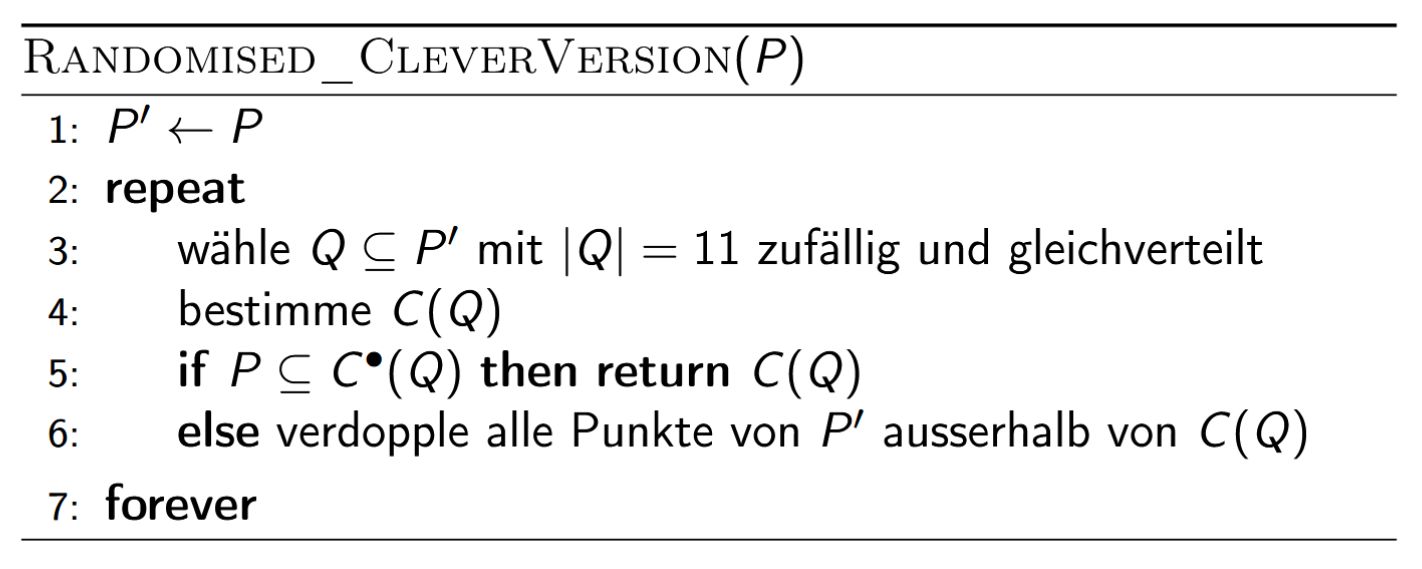
In jeder Runde wird die Stichprobe aus
\(P'\) (nicht \(P\)) gezogen, geprüft wird gegen
\(P\), und bei Misserfolg werden
die Punkte aus \(P'\) ausserhalb von \(C(Q)\) verdoppelt (Vielfachheit).
Back
ETH::2._Semester::A&W::3._Algorithmen_-_Highlights::1._Graphenalgorithmen::4._Kleinster_umschliessender_Kreis::3._Clarkson-Algorithmus
In jeder Runde wird die Stichprobe aus
\(P'\) (nicht \(P\)) gezogen, geprüft wird gegen
\(P\), und bei Misserfolg werden
die Punkte aus \(P'\) ausserhalb von \(C(Q)\) verdoppelt (Vielfachheit).
Setzt man voraus, dass die Wahl von \(Q\) in \(O(n)\) möglich ist, so kostet jede Runde \(O(n)\). Idee von [Clarkson '95].
Field-by-field Comparison
| Field |
Before |
After |
| Text |
|
<img src="paste-c06c475b4dec3b431734591273342bcaada9ffb3.jpg"><br><br>In jeder Runde wird die Stichprobe aus {{c1::\(P'\) (nicht \(P\))}} gezogen, geprüft wird gegen {{c2::\(P\)}}, und bei Misserfolg werden {{c3::die Punkte aus \(P'\) ausserhalb von \(C(Q)\) verdoppelt (Vielfachheit)}}. |
| Extra |
|
Setzt man voraus, dass die Wahl von \(Q\) in \(O(n)\) möglich ist, so kostet jede Runde \(O(n)\). Idee von [Clarkson '95]. |
Tags:
ETH::2._Semester::A&W::3._Algorithmen_-_Highlights::1._Graphenalgorithmen::4._Kleinster_umschliessender_Kreis::3._Clarkson-Algorithmus
Note 41: ETH::2. Semester::A&W
Deck: ETH::2. Semester::A&W
Note Type: Horvath Classic
GUID: kKQ$vT!!Iq
added
Previous
Note did not exist
New Note
Front
ETH::2._Semester::A&W::3._Algorithmen_-_Highlights::1._Graphenalgorithmen::4._Kleinster_umschliessender_Kreis::2._Erste_Algorithmen
CompleteEnumeration(\(P\)).
Beschreibe das Vorgehen und die Laufzeit des naiven Enumerationsalgorithmus für \(C(P)\).
Back
ETH::2._Semester::A&W::3._Algorithmen_-_Highlights::1._Graphenalgorithmen::4._Kleinster_umschliessender_Kreis::2._Erste_Algorithmen
CompleteEnumeration(\(P\)).
Beschreibe das Vorgehen und die Laufzeit des naiven Enumerationsalgorithmus für \(C(P)\).
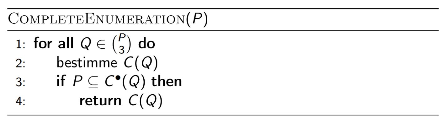
Man durchläuft \(\binom{n}{3}\) Mengen \(Q\), berechnet jedes \(C(Q)\) in \(O(1)\) und prüft \(P \subseteq C^{\bullet}(Q)\) in \(O(n)\).
Laufzeit: \(O(n^4)\).
Field-by-field Comparison
| Field |
Before |
After |
| Front |
|
<b>CompleteEnumeration(\(P\)).</b><br>Beschreibe das Vorgehen und die Laufzeit des naiven Enumerationsalgorithmus für \(C(P)\). |
| Back |
|
<img src="paste-90c1a320650f09fb193c9f69076b17b4979e28a5.jpg"><br><br>Man durchläuft \(\binom{n}{3}\) Mengen \(Q\), berechnet jedes \(C(Q)\) in \(O(1)\) und prüft \(P \subseteq C^{\bullet}(Q)\) in \(O(n)\).<br><br>Laufzeit: \(O(n^4)\). |
Tags:
ETH::2._Semester::A&W::3._Algorithmen_-_Highlights::1._Graphenalgorithmen::4._Kleinster_umschliessender_Kreis::2._Erste_Algorithmen
Note 42: ETH::2. Semester::A&W
Deck: ETH::2. Semester::A&W
Note Type: Horvath Cloze
GUID: niQo~f{zrh
added
Previous
Note did not exist
New Note
Front
ETH::2._Semester::A&W::3._Algorithmen_-_Highlights::1._Graphenalgorithmen::5._Konvexe_Hülle
LocalRepair (Eingabe \((p_1, \ldots, p_n)\) nach \(x\)-Koordinate sortiert).
Zwei Sweeps: erst
unterer Rand, links nach rechts, dann
oberer Rand, rechts nach links; jeweils wird \(q_i\) per Pop entfernt, solange \(p_i\) rechts von \(q_{h-1}, q_h\) liegt:
LocalRepair(p₁, ..., p_n):   # sortiert
  q₀ ← p₁; h ← 0
  for i ← 2 to n:              # unterer Rand, links→rechts
    while h > 0 and p_i rechts von q_{h-1}, q_h:
      h ← h - 1
    h ← h + 1; q_h ← p_i
  h' ← h
  for i ← n-1 downto 1:        # oberer Rand, rechts→links
    while h > h' and p_i rechts von q_{h-1}, q_h:
      h ← h - 1
    h ← h + 1; q_h ← p_i
  return (q₀, q₁, ..., q_{h-1})
Back
ETH::2._Semester::A&W::3._Algorithmen_-_Highlights::1._Graphenalgorithmen::5._Konvexe_Hülle
LocalRepair (Eingabe \((p_1, \ldots, p_n)\) nach \(x\)-Koordinate sortiert).
Zwei Sweeps: erst
unterer Rand, links nach rechts, dann
oberer Rand, rechts nach links; jeweils wird \(q_i\) per Pop entfernt, solange \(p_i\) rechts von \(q_{h-1}, q_h\) liegt:
LocalRepair(p₁, ..., p_n):   # sortiert
  q₀ ← p₁; h ← 0
  for i ← 2 to n:              # unterer Rand, links→rechts
    while h > 0 and p_i rechts von q_{h-1}, q_h:
      h ← h - 1
    h ← h + 1; q_h ← p_i
  h' ← h
  for i ← n-1 downto 1:        # oberer Rand, rechts→links
    while h > h' and p_i rechts von q_{h-1}, q_h:
      h ← h - 1
    h ← h + 1; q_h ← p_i
  return (q₀, q₁, ..., q_{h-1})
Nach der ersten Schleife ist \((q_0, \ldots, q_h)\) die untere konvexe Hülle von \(\{p_1, \ldots, p_n\}\); die Schranke \(h > h'\) verhindert, dass der obere Sweep in den unteren Rand hineinläuft.
Field-by-field Comparison
| Field |
Before |
After |
| Text |
|
<b>LocalRepair</b> (Eingabe \((p_1, \ldots, p_n)\) nach \(x\)-Koordinate sortiert).<br>Zwei Sweeps: erst {{c1::unterer Rand, links nach rechts}}, dann {{c2::oberer Rand, rechts nach links}}; jeweils wird \(q_i\) per Pop entfernt, solange \(p_i\) rechts von \(q_{h-1}, q_h\) liegt:<pre>LocalRepair(p₁, ..., p_n): # sortiert
q₀ ← p₁; h ← 0
for i ← 2 to n: # unterer Rand, links→rechts
while h > 0 and p_i rechts von q_{h-1}, q_h:
h ← h - 1
h ← h + 1; q_h ← p_i
h' ← h
for i ← n-1 downto 1: # oberer Rand, rechts→links
while h > h' and p_i rechts von q_{h-1}, q_h:
h ← h - 1
h ← h + 1; q_h ← p_i
return (q₀, q₁, ..., q_{h-1})</pre> |
| Extra |
|
Nach der ersten Schleife ist \((q_0, \ldots, q_h)\) die untere konvexe Hülle von \(\{p_1, \ldots, p_n\}\); die Schranke \(h > h'\) verhindert, dass der obere Sweep in den unteren Rand hineinläuft. |
Tags:
ETH::2._Semester::A&W::3._Algorithmen_-_Highlights::1._Graphenalgorithmen::5._Konvexe_Hülle
Note 43: ETH::2. Semester::A&W
Deck: ETH::2. Semester::A&W
Note Type: Horvath Cloze
GUID: p:|%b(`#o{
added
Previous
Note did not exist
New Note
Front
ETH::2._Semester::A&W::3._Algorithmen_-_Highlights::1._Graphenalgorithmen::5._Konvexe_Hülle
Orientierungstest für allgemeines \(q\) (nicht im Ursprung).
\(p\) liegt links von \(q, r\) \(\iff\) \(p - q\) liegt links von \(o,\ r - q\) \(\iff\)\[(r_x - q_x)(p_y - q_y) - (p_x - q_x)(r_y - q_y) > 0.\]
Back
ETH::2._Semester::A&W::3._Algorithmen_-_Highlights::1._Graphenalgorithmen::5._Konvexe_Hülle
Orientierungstest für allgemeines \(q\) (nicht im Ursprung).
\(p\) liegt links von \(q, r\) \(\iff\) \(p - q\) liegt links von \(o,\ r - q\) \(\iff\)\[(r_x - q_x)(p_y - q_y) - (p_x - q_x)(r_y - q_y) > 0.\]
Field-by-field Comparison
| Field |
Before |
After |
| Text |
|
<b>Orientierungstest für allgemeines \(q\) (nicht im Ursprung).</b><br>\(p\) liegt links von \(q, r\) \(\iff\) {{c1::\(p - q\) liegt links von \(o,\ r - q\)}} \(\iff\)\[{{c2::(r_x - q_x)(p_y - q_y) - (p_x - q_x)(r_y - q_y) > 0}}.\] |
Tags:
ETH::2._Semester::A&W::3._Algorithmen_-_Highlights::1._Graphenalgorithmen::5._Konvexe_Hülle
Note 44: ETH::2. Semester::A&W
Deck: ETH::2. Semester::A&W
Note Type: Horvath Cloze
GUID: qzy.kvo
added
Previous
Note did not exist
New Note
Front
ETH::2._Semester::A&W::3._Algorithmen_-_Highlights::1._Graphenalgorithmen::5._Konvexe_Hülle
JarvisWrap: Umgang mit Degeneriertheiten (Kollinearitäten, gleiche \(x\)-Koordinaten, Duplikate).
- Startpunkt \(q_0\): nimm den Punkt mit lexikographisch kleinster Koordinate (unter kleinster \(x\)-Koordinate den mit kleinster \(y\)-Koordinate).
- Test "\(p\) rechts von \(q, q_{\text{next} }\)" ersetzen durch: rechts von \(q, q_{\text{next} }\) {{c2::oder (\(p\) auf der Geraden durch \(q, q_{\text{next} }\) und \(|qp| > |q q_{\text{next} }|\))}}.
- Punkte sind i.d.R. nicht einmal verschieden (z.B. in einem Feld gegeben).
Back
ETH::2._Semester::A&W::3._Algorithmen_-_Highlights::1._Graphenalgorithmen::5._Konvexe_Hülle
JarvisWrap: Umgang mit Degeneriertheiten (Kollinearitäten, gleiche \(x\)-Koordinaten, Duplikate).
- Startpunkt \(q_0\): nimm den Punkt mit lexikographisch kleinster Koordinate (unter kleinster \(x\)-Koordinate den mit kleinster \(y\)-Koordinate).
- Test "\(p\) rechts von \(q, q_{\text{next} }\)" ersetzen durch: rechts von \(q, q_{\text{next} }\) {{c2::oder (\(p\) auf der Geraden durch \(q, q_{\text{next} }\) und \(|qp| > |q q_{\text{next} }|\))}}.
- Punkte sind i.d.R. nicht einmal verschieden (z.B. in einem Feld gegeben).
Software ohne Berücksichtigung dieser Fälle hat geringen praktischen Nutzen.
Field-by-field Comparison
| Field |
Before |
After |
| Text |
|
<b>JarvisWrap: Umgang mit Degeneriertheiten</b> (Kollinearitäten, gleiche \(x\)-Koordinaten, Duplikate).<br><ul><li>Startpunkt \(q_0\): nimm den Punkt mit {{c1::lexikographisch kleinster Koordinate}} (unter kleinster \(x\)-Koordinate den mit kleinster \(y\)-Koordinate).</li><li>Test "\(p\) rechts von \(q, q_{\text{next} }\)" ersetzen durch: rechts von \(q, q_{\text{next} }\) {{c2::oder (\(p\) auf der Geraden durch \(q, q_{\text{next} }\) und \(|qp| > |q q_{\text{next} }|\))}}.</li><li>Punkte sind i.d.R. {{c3::nicht einmal verschieden}} (z.B. in einem Feld gegeben).</li></ul> |
| Extra |
|
Software ohne Berücksichtigung dieser Fälle hat geringen praktischen Nutzen. |
Tags:
ETH::2._Semester::A&W::3._Algorithmen_-_Highlights::1._Graphenalgorithmen::5._Konvexe_Hülle
Note 45: ETH::2. Semester::A&W
Deck: ETH::2. Semester::A&W
Note Type: Horvath Cloze
GUID: rp8q^uUl`4
added
Previous
Note did not exist
New Note
Front
ETH::2._Semester::A&W::3._Algorithmen_-_Highlights::1._Graphenalgorithmen::5._Konvexe_Hülle
Lokale Bedingung (lokal konvex).
Für ein Polygon \((q_0, q_1, \ldots, q_{h-1})\) lautet die lokale Prüfung (Indizes \(\bmod\, h\)):\[\forall i,\ 1 \leq i \leq h: \quad {{c1::q_{i+1} \text{ liegt links von } q_{i-1}, q_i}}.\]
Back
ETH::2._Semester::A&W::3._Algorithmen_-_Highlights::1._Graphenalgorithmen::5._Konvexe_Hülle
Lokale Bedingung (lokal konvex).
Für ein Polygon \((q_0, q_1, \ldots, q_{h-1})\) lautet die lokale Prüfung (Indizes \(\bmod\, h\)):\[\forall i,\ 1 \leq i \leq h: \quad {{c1::q_{i+1} \text{ liegt links von } q_{i-1}, q_i}}.\]
Diese lokale Eigenschaft ist die Grundlage des LocalRepair-Ansatzes: konvexifiziere, bis sie überall gilt.
Field-by-field Comparison
| Field |
Before |
After |
| Text |
|
<b>Lokale Bedingung (lokal konvex).</b><br>Für ein Polygon \((q_0, q_1, \ldots, q_{h-1})\) lautet die lokale Prüfung (Indizes \(\bmod\, h\)):\[\forall i,\ 1 \leq i \leq h: \quad {{c1::q_{i+1} \text{ liegt links von } q_{i-1}, q_i}}.\] |
| Extra |
|
Diese lokale Eigenschaft ist die Grundlage des LocalRepair-Ansatzes: konvexifiziere, bis sie überall gilt. |
Tags:
ETH::2._Semester::A&W::3._Algorithmen_-_Highlights::1._Graphenalgorithmen::5._Konvexe_Hülle
Note 46: ETH::2. Semester::A&W
Deck: ETH::2. Semester::A&W
Note Type: Horvath Cloze
GUID: smm|mYgkUr
added
Previous
Note did not exist
New Note
Front
ETH::2._Semester::A&W::3._Algorithmen_-_Highlights::1._Graphenalgorithmen::5._Konvexe_Hülle
JarvisWrap: Laufzeit-Spezialfälle.Aus \(O(nh)\) folgt:
- Da \(h \leq n\), läuft JarvisWrap in \(O(n^2)\) (statt \(O(n^3)\) beim naiven Ansatz).
- Ist \(h = O(1)\) (z.B. \(\operatorname{conv}(P)\) ein Dreieck), so \(O(n)\).
Back
ETH::2._Semester::A&W::3._Algorithmen_-_Highlights::1._Graphenalgorithmen::5._Konvexe_Hülle
JarvisWrap: Laufzeit-Spezialfälle.Aus \(O(nh)\) folgt:
- Da \(h \leq n\), läuft JarvisWrap in \(O(n^2)\) (statt \(O(n^3)\) beim naiven Ansatz).
- Ist \(h = O(1)\) (z.B. \(\operatorname{conv}(P)\) ein Dreieck), so \(O(n)\).
Field-by-field Comparison
| Field |
Before |
After |
| Text |
|
<b>JarvisWrap: Laufzeit-Spezialfälle.</b><br>Aus \(O(nh)\) folgt:<br><ul><li>Da \(h \leq n\), läuft JarvisWrap in {{c1::\(O(n^2)\)}} (statt \(O(n^3)\) beim naiven Ansatz).</li><li>Ist \(h = O(1)\) (z.B. \(\operatorname{conv}(P)\) ein Dreieck), so {{c2::\(O(n)\)}}.</li></ul> |
Tags:
ETH::2._Semester::A&W::3._Algorithmen_-_Highlights::1._Graphenalgorithmen::5._Konvexe_Hülle
Note 47: ETH::2. Semester::A&W
Deck: ETH::2. Semester::A&W
Note Type: Horvath Cloze
GUID: tJY%fGS%zk
added
Previous
Note did not exist
New Note
Front
ETH::2._Semester::A&W::3._Algorithmen_-_Highlights::1._Graphenalgorithmen::4._Kleinster_umschliessender_Kreis::3._Clarkson-Algorithmus
Anmerkungen zum Clarkson-Algorithmus.- Der Algorithmus funktioniert auch für die kleinste umschliessende Kugel (oder Ellipse) in allen Dimensionen, mit anderen Konstanten statt der \(11\). Bei fixer Dimension bleibt die Laufzeit \(O(n \log n)\).
- Es gibt auch einfache randomisierte und sogar deterministische Linearzeit-Algorithmen (in jeder fixen Dimension).
Back
ETH::2._Semester::A&W::3._Algorithmen_-_Highlights::1._Graphenalgorithmen::4._Kleinster_umschliessender_Kreis::3._Clarkson-Algorithmus
Anmerkungen zum Clarkson-Algorithmus.- Der Algorithmus funktioniert auch für die kleinste umschliessende Kugel (oder Ellipse) in allen Dimensionen, mit anderen Konstanten statt der \(11\). Bei fixer Dimension bleibt die Laufzeit \(O(n \log n)\).
- Es gibt auch einfache randomisierte und sogar deterministische Linearzeit-Algorithmen (in jeder fixen Dimension).
Idee von [Clarkson '95].
Field-by-field Comparison
| Field |
Before |
After |
| Text |
|
<b>Anmerkungen zum Clarkson-Algorithmus.</b><br><ul><li>Der Algorithmus funktioniert auch für die kleinste umschliessende Kugel (oder Ellipse) in {{c1::allen Dimensionen}}, mit anderen Konstanten statt der \(11\). Bei {{c2::fixer Dimension}} bleibt die Laufzeit \(O(n \log n)\).</li><li>Es gibt auch einfache randomisierte und sogar deterministische {{c3::Linearzeit}}-Algorithmen (in jeder fixen Dimension).</li></ul> |
| Extra |
|
Idee von [Clarkson '95]. |
Tags:
ETH::2._Semester::A&W::3._Algorithmen_-_Highlights::1._Graphenalgorithmen::4._Kleinster_umschliessender_Kreis::3._Clarkson-Algorithmus
Note 48: ETH::2. Semester::A&W
Deck: ETH::2. Semester::A&W
Note Type: Horvath Cloze
GUID: u2{>}8MB*o
added
Previous
Note did not exist
New Note
Front
ETH::2._Semester::A&W::3._Algorithmen_-_Highlights::1._Graphenalgorithmen::5._Konvexe_Hülle
Ordnung \(\prec_q\) um einen Punkt.
Für gegebenes \(q \in P\) definiert man auf \(P \setminus \{q\}\):\[p_1 \prec_q p_2 :\iff {{c1::p_1 \text{ liegt rechts von } q, p_2}}.\]
Back
ETH::2._Semester::A&W::3._Algorithmen_-_Highlights::1._Graphenalgorithmen::5._Konvexe_Hülle
Ordnung \(\prec_q\) um einen Punkt.
Für gegebenes \(q \in P\) definiert man auf \(P \setminus \{q\}\):\[p_1 \prec_q p_2 :\iff {{c1::p_1 \text{ liegt rechts von } q, p_2}}.\]
Field-by-field Comparison
| Field |
Before |
After |
| Text |
|
<b>Ordnung \(\prec_q\) um einen Punkt.</b><br>Für gegebenes \(q \in P\) definiert man auf \(P \setminus \{q\}\):\[p_1 \prec_q p_2 :\iff {{c1::p_1 \text{ liegt rechts von } q, p_2}}.\] |
Tags:
ETH::2._Semester::A&W::3._Algorithmen_-_Highlights::1._Graphenalgorithmen::5._Konvexe_Hülle
Note 49: ETH::2. Semester::A&W
Deck: ETH::2. Semester::A&W
Note Type: Horvath Classic
GUID: vr2QG*.a{<
added
Previous
Note did not exist
New Note
Front
ETH::2._Semester::A&W::3._Algorithmen_-_Highlights::1._Graphenalgorithmen::4._Kleinster_umschliessender_Kreis::5._Laufzeitanalyse
Satz (Clarkson-Algorithmus).
Welche erwartete Laufzeit hat der Algorithmus, und wie folgt sie aus \(\Pr[T \geq k] \leq 0.993^k n\)?
Back
ETH::2._Semester::A&W::3._Algorithmen_-_Highlights::1._Graphenalgorithmen::4._Kleinster_umschliessender_Kreis::5._Laufzeitanalyse
Satz (Clarkson-Algorithmus).
Welche erwartete Laufzeit hat der Algorithmus, und wie folgt sie aus \(\Pr[T \geq k] \leq 0.993^k n\)?
Der Algorithmus berechnet \(C(P)\) in erwartet \(O(n \log n)\) Zeit.
Proof Included. Die Laufzeit ist \(O(nT)\). Setze \(k_0 := \lfloor -\log_{0.993} n \rfloor = O(\log n)\). Dann\[\begin{gathered}\mathbb{E}[T] = \sum_{k \geq 1} \Pr[T \geq k] \;\leq\; \sum_{k=1}^{k_0} 1 \;+\; \sum_{k > k_0} 0.993^{\,k} n \\= k_0 \;+\; \underbrace{\sum_{k' \geq 0} 0.993^{\,k'} \cdot 0.993^{\,k_0 + 1} n}_{\leq\, O(1)} \;=\; k_0 + O(1) = O(\log n).\end{gathered}\]Also \(\mathbb{E}[\text{Laufzeit}] = O(n \cdot \mathbb{E}[T]) = O(n \log n)\).
Field-by-field Comparison
| Field |
Before |
After |
| Front |
|
<b>Satz (Clarkson-Algorithmus).</b><br>Welche erwartete Laufzeit hat der Algorithmus, und wie folgt sie aus \(\Pr[T \geq k] \leq 0.993^k n\)? |
| Back |
|
Der Algorithmus berechnet \(C(P)\) in erwartet \(O(n \log n)\) Zeit.<br><br>Proof Included. Die Laufzeit ist \(O(nT)\). Setze \(k_0 := \lfloor -\log_{0.993} n \rfloor = O(\log n)\). Dann\[\begin{gathered}\mathbb{E}[T] = \sum_{k \geq 1} \Pr[T \geq k] \;\leq\; \sum_{k=1}^{k_0} 1 \;+\; \sum_{k > k_0} 0.993^{\,k} n \\= k_0 \;+\; \underbrace{\sum_{k' \geq 0} 0.993^{\,k'} \cdot 0.993^{\,k_0 + 1} n}_{\leq\, O(1)} \;=\; k_0 + O(1) = O(\log n).\end{gathered}\]Also \(\mathbb{E}[\text{Laufzeit}] = O(n \cdot \mathbb{E}[T]) = O(n \log n)\). |
Tags:
ETH::2._Semester::A&W::3._Algorithmen_-_Highlights::1._Graphenalgorithmen::4._Kleinster_umschliessender_Kreis::5._Laufzeitanalyse
Note 50: ETH::2. Semester::A&W
Deck: ETH::2. Semester::A&W
Note Type: Horvath Cloze
GUID: x$AVm(?T-w
added
Previous
Note did not exist
New Note
Front
ETH::2._Semester::A&W::3._Algorithmen_-_Highlights::1._Graphenalgorithmen::4._Kleinster_umschliessender_Kreis::5._Laufzeitanalyse
Schranke für \(\Pr[T \geq k]\).
Sei \(T\) die Rundenzahl und \(X_k = |P'|\) nach \(\min\{T, k\}\) Runden. Aus \(X_k \geq 2^{k/3}\) (falls \(T \geq k\)) und \(\mathbb{E}[X_k] \leq (\tfrac54)^k n\) folgt\[2^{k/3} \Pr[T \geq k] \;\leq\; \mathbb{E}[X_k] \;\leq\; \left(\tfrac54\right)^k n,\]also\[\Pr[T \geq k] \;\leq\; {{c1::\left(\frac{5}{4 \cdot 2^{1/3}}\right)^k n \;\leq\; 0.993^{\,k}\, n}}.\]
Back
ETH::2._Semester::A&W::3._Algorithmen_-_Highlights::1._Graphenalgorithmen::4._Kleinster_umschliessender_Kreis::5._Laufzeitanalyse
Schranke für \(\Pr[T \geq k]\).
Sei \(T\) die Rundenzahl und \(X_k = |P'|\) nach \(\min\{T, k\}\) Runden. Aus \(X_k \geq 2^{k/3}\) (falls \(T \geq k\)) und \(\mathbb{E}[X_k] \leq (\tfrac54)^k n\) folgt\[2^{k/3} \Pr[T \geq k] \;\leq\; \mathbb{E}[X_k] \;\leq\; \left(\tfrac54\right)^k n,\]also\[\Pr[T \geq k] \;\leq\; {{c1::\left(\frac{5}{4 \cdot 2^{1/3}}\right)^k n \;\leq\; 0.993^{\,k}\, n}}.\]
Der entscheidende Schritt: \(\mathbb{E}[X_k] \geq \mathbb{E}[X_k \mid T \geq k]\cdot \Pr[T \geq k] \geq 2^{k/3}\Pr[T \geq k]\). Für \(k \geq -\log_{0.993} n\) wird die Schranke \(\leq 1\).
Field-by-field Comparison
| Field |
Before |
After |
| Text |
|
<b>Schranke für \(\Pr[T \geq k]\).</b><br>Sei \(T\) die Rundenzahl und \(X_k = |P'|\) nach \(\min\{T, k\}\) Runden. Aus \(X_k \geq 2^{k/3}\) (falls \(T \geq k\)) und \(\mathbb{E}[X_k] \leq (\tfrac54)^k n\) folgt\[2^{k/3} \Pr[T \geq k] \;\leq\; \mathbb{E}[X_k] \;\leq\; \left(\tfrac54\right)^k n,\]also\[\Pr[T \geq k] \;\leq\; {{c1::\left(\frac{5}{4 \cdot 2^{1/3}}\right)^k n \;\leq\; 0.993^{\,k}\, n}}.\] |
| Extra |
|
Der entscheidende Schritt: \(\mathbb{E}[X_k] \geq \mathbb{E}[X_k \mid T \geq k]\cdot \Pr[T \geq k] \geq 2^{k/3}\Pr[T \geq k]\). Für \(k \geq -\log_{0.993} n\) wird die Schranke \(\leq 1\). |
Tags:
ETH::2._Semester::A&W::3._Algorithmen_-_Highlights::1._Graphenalgorithmen::4._Kleinster_umschliessender_Kreis::5._Laufzeitanalyse
Note 51: ETH::2. Semester::A&W
Deck: ETH::2. Semester::A&W
Note Type: Horvath Cloze
GUID: y5q+v+k~r2
added
Previous
Note did not exist
New Note
Front
ETH::2._Semester::A&W::3._Algorithmen_-_Highlights::1._Graphenalgorithmen::5._Konvexe_Hülle
Erster naiver Ansatz für ConvexHull.
Gehe durch jedes der \(n(n-1)\) geordneten Paare \(qr\) und prüfe per Orientierungstest über alle \(n - 2\) übrigen Punkte, ob \(qr\) eine Randkante ist.
Laufzeit zum Finden aller Randkanten: \(O(n^3)\) (danach nur noch korrekt aneinanderreihen).
Back
ETH::2._Semester::A&W::3._Algorithmen_-_Highlights::1._Graphenalgorithmen::5._Konvexe_Hülle
Erster naiver Ansatz für ConvexHull.
Gehe durch jedes der \(n(n-1)\) geordneten Paare \(qr\) und prüfe per Orientierungstest über alle \(n - 2\) übrigen Punkte, ob \(qr\) eine Randkante ist.
Laufzeit zum Finden aller Randkanten: \(O(n^3)\) (danach nur noch korrekt aneinanderreihen).
Field-by-field Comparison
| Field |
Before |
After |
| Text |
|
<b>Erster naiver Ansatz für ConvexHull.</b><br>Gehe durch jedes der {{c1::\(n(n-1)\)}} geordneten Paare \(qr\) und prüfe per Orientierungstest über alle \(n - 2\) übrigen Punkte, {{c2::ob \(qr\) eine Randkante ist}}.<br><br>Laufzeit zum Finden aller Randkanten: {{c3::\(O(n^3)\)}} (danach nur noch korrekt aneinanderreihen). |
Tags:
ETH::2._Semester::A&W::3._Algorithmen_-_Highlights::1._Graphenalgorithmen::5._Konvexe_Hülle
Note 52: ETH::2. Semester::A&W
Deck: ETH::2. Semester::A&W
Note Type: Horvath Cloze
GUID: yr2,_1,&|p
added
Previous
Note did not exist
New Note
Front
ETH::2._Semester::A&W::3._Algorithmen_-_Highlights::1._Graphenalgorithmen::4._Kleinster_umschliessender_Kreis::1._Grundlagen
SmallEnclDisk-Problem.
Gegeben eine endliche Punktemenge \(P \subseteq \mathbb{R}^2\), bestimme den Kreis kleinsten Radius, der \(P\) umschliesst.
Für einen Kreis \(C\) bezeichnet \(C^{\bullet}\) die geschlossene, von \(C\) berandete Kreisscheibe. Wir sagen \(C\) umschliesst \(P\), falls {{c3::\(P \subseteq C^{\bullet}\)}}.
Back
ETH::2._Semester::A&W::3._Algorithmen_-_Highlights::1._Graphenalgorithmen::4._Kleinster_umschliessender_Kreis::1._Grundlagen
SmallEnclDisk-Problem.
Gegeben eine endliche Punktemenge \(P \subseteq \mathbb{R}^2\), bestimme den Kreis kleinsten Radius, der \(P\) umschliesst.
Für einen Kreis \(C\) bezeichnet \(C^{\bullet}\) die geschlossene, von \(C\) berandete Kreisscheibe. Wir sagen \(C\) umschliesst \(P\), falls {{c3::\(P \subseteq C^{\bullet}\)}}.
Punkte in \(P\) dürfen also auf dem Rand \(C\) liegen.
Field-by-field Comparison
| Field |
Before |
After |
| Text |
|
<b>SmallEnclDisk-Problem.</b><br>Gegeben eine endliche Punktemenge \(P \subseteq \mathbb{R}^2\), bestimme {{c1::den Kreis kleinsten Radius, der \(P\) umschliesst}}.<br><br>Für einen Kreis \(C\) bezeichnet \(C^{\bullet}\) {{c2::die geschlossene, von \(C\) berandete Kreisscheibe}}. Wir sagen \(C\) umschliesst \(P\), falls {{c3::\(P \subseteq C^{\bullet}\)}}. |
| Extra |
|
Punkte in \(P\) dürfen also auf dem Rand \(C\) liegen. |
Tags:
ETH::2._Semester::A&W::3._Algorithmen_-_Highlights::1._Graphenalgorithmen::4._Kleinster_umschliessender_Kreis::1._Grundlagen
Note 53: ETH::2. Semester::A&W
Deck: ETH::2. Semester::A&W
Note Type: Horvath Cloze
GUID: zks9N%wc9R
added
Previous
Note did not exist
New Note
Front
ETH::2._Semester::A&W::3._Algorithmen_-_Highlights::1._Graphenalgorithmen::5._Konvexe_Hülle
ConvexHull-Problem.
Gegeben eine endliche Punktmenge {{c1::\(P \subseteq \mathbb{R}^2\)}}, bestimme die konvexe Hülle von \(P\).
In der Praxis heisst das konkret: bestimme {{c3::die Ecken des \(\operatorname{conv}(P)\) umrandenden Polygons, in der Reihenfolge gegen den Uhrzeigersinn}}.
Back
ETH::2._Semester::A&W::3._Algorithmen_-_Highlights::1._Graphenalgorithmen::5._Konvexe_Hülle
ConvexHull-Problem.
Gegeben eine endliche Punktmenge {{c1::\(P \subseteq \mathbb{R}^2\)}}, bestimme die konvexe Hülle von \(P\).
In der Praxis heisst das konkret: bestimme {{c3::die Ecken des \(\operatorname{conv}(P)\) umrandenden Polygons, in der Reihenfolge gegen den Uhrzeigersinn}}.
Field-by-field Comparison
| Field |
Before |
After |
| Text |
|
<b>ConvexHull-Problem.</b><br>Gegeben eine endliche Punktmenge {{c1::\(P \subseteq \mathbb{R}^2\)}}, bestimme {{c2::die konvexe Hülle von \(P\)}}.<br><br>In der Praxis heisst das konkret: bestimme {{c3::die Ecken des \(\operatorname{conv}(P)\) umrandenden Polygons, in der Reihenfolge gegen den Uhrzeigersinn}}. |
Tags:
ETH::2._Semester::A&W::3._Algorithmen_-_Highlights::1._Graphenalgorithmen::5._Konvexe_Hülle
Note 54: ETH::2. Semester::A&W
Deck: ETH::2. Semester::A&W
Note Type: Horvath Cloze
GUID: zni~6&*S9I
added
Previous
Note did not exist
New Note
Front
ETH::2._Semester::A&W::3._Algorithmen_-_Highlights::1._Graphenalgorithmen::5._Konvexe_Hülle
Startpunkt und FindNext.Wähle \(q_0 :=\)
Punkt mit kleinster \(x\)-Koordinate in \(P\); dieser ist sicher
eine Ecke der konvexen Hülle.
FindNext(q) findet den nächsten Hüllenpunkt, indem es startend mit beliebigem \(p_0\) jeden Punkt durchgeht und \(q_{\text{next} }\) ersetzt, sobald {{c3::\(p\) rechts von \(q, q_{\text{next} }\) liegt}}:
FindNext(q):
  wähle p₀ ∈ P \ {q} beliebig
  q_next ← p₀
  for all p ∈ P \ {q, p₀}:
    if p rechts von q, q_next:
      q_next ← p
  return q_next
Back
ETH::2._Semester::A&W::3._Algorithmen_-_Highlights::1._Graphenalgorithmen::5._Konvexe_Hülle
Startpunkt und FindNext.Wähle \(q_0 :=\)
Punkt mit kleinster \(x\)-Koordinate in \(P\); dieser ist sicher
eine Ecke der konvexen Hülle.
FindNext(q) findet den nächsten Hüllenpunkt, indem es startend mit beliebigem \(p_0\) jeden Punkt durchgeht und \(q_{\text{next} }\) ersetzt, sobald {{c3::\(p\) rechts von \(q, q_{\text{next} }\) liegt}}:
FindNext(q):
  wähle p₀ ∈ P \ {q} beliebig
  q_next ← p₀
  for all p ∈ P \ {q, p₀}:
    if p rechts von q, q_next:
      q_next ← p
  return q_next
Field-by-field Comparison
| Field |
Before |
After |
| Text |
|
<b>Startpunkt und FindNext.</b><br>Wähle \(q_0 :=\) {{c1::Punkt mit kleinster \(x\)-Koordinate in \(P\)}}; dieser ist sicher {{c2::eine Ecke der konvexen Hülle}}.<br><br><code>FindNext(q)</code> findet den nächsten Hüllenpunkt, indem es startend mit beliebigem \(p_0\) jeden Punkt durchgeht und \(q_{\text{next} }\) ersetzt, sobald {{c3::\(p\) rechts von \(q, q_{\text{next} }\) liegt}}:<pre>FindNext(q):
wähle p₀ ∈ P \ {q} beliebig
q_next ← p₀
for all p ∈ P \ {q, p₀}:
if p rechts von q, q_next:
q_next ← p
return q_next</pre> |
Tags:
ETH::2._Semester::A&W::3._Algorithmen_-_Highlights::1._Graphenalgorithmen::5._Konvexe_Hülle
Note 55: ETH::2. Semester::A&W
Deck: ETH::2. Semester::A&W
Note Type: Horvath Cloze
GUID: }z)}~szKhW
added
Previous
Note did not exist
New Note
Front
ETH::2._Semester::A&W::3._Algorithmen_-_Highlights::1._Graphenalgorithmen::5._Konvexe_Hülle
Konvexe Hülle \(\operatorname{conv}(S)\).
Die konvexe Hülle einer Menge \(S \subseteq \mathbb{R}^d\) ist der Schnitt aller konvexen Mengen, die \(S\) enthalten:\[\operatorname{conv}(S) := {{c1::\bigcap_{S \subseteq C \subseteq \mathbb{R}^d,\ C \text{ konvex} } C}}.\]Äquivalent: (i) der Schnitt aller Halbebenen, die \(S\) enthalten, (ii) die kleinste konvexe Menge, die \(S\) enthält.
Back
ETH::2._Semester::A&W::3._Algorithmen_-_Highlights::1._Graphenalgorithmen::5._Konvexe_Hülle
Konvexe Hülle \(\operatorname{conv}(S)\).
Die konvexe Hülle einer Menge \(S \subseteq \mathbb{R}^d\) ist der Schnitt aller konvexen Mengen, die \(S\) enthalten:\[\operatorname{conv}(S) := {{c1::\bigcap_{S \subseteq C \subseteq \mathbb{R}^d,\ C \text{ konvex} } C}}.\]Äquivalent: (i) der Schnitt aller Halbebenen, die \(S\) enthalten, (ii) die kleinste konvexe Menge, die \(S\) enthält.
Field-by-field Comparison
| Field |
Before |
After |
| Text |
|
<b>Konvexe Hülle \(\operatorname{conv}(S)\).</b><br>Die konvexe Hülle einer Menge \(S \subseteq \mathbb{R}^d\) ist {{c1::der Schnitt aller konvexen Mengen, die \(S\) enthalten}}:\[\operatorname{conv}(S) := {{c1::\bigcap_{S \subseteq C \subseteq \mathbb{R}^d,\ C \text{ konvex} } C}}.\]Äquivalent: (i) {{c2::der Schnitt aller Halbebenen, die \(S\) enthalten}}, (ii) {{c3::die kleinste konvexe Menge, die \(S\) enthält}}. |
Tags:
ETH::2._Semester::A&W::3._Algorithmen_-_Highlights::1._Graphenalgorithmen::5._Konvexe_Hülle
Note 56: ETH::2. Semester::Analysis
Deck: ETH::2. Semester::Analysis
Note Type: Horvath Classic
GUID: %CZXZP?p{Y
added
Previous
Note did not exist
New Note
Front
ETH::2._Semester::Analysis::5._Differentialrechnung::2._Differenzierbarkeit ETH::2._Semester::Analysis::Serie::8
Welche Aussage gilt für eine differenzierbare Funktion \(f : \mathbb{R} \rightarrow \mathbb{R}\)?
- Ist \(f\) gerade, so ist die Ableitung \(f'\) gerade.
- Ist \(f\) gerade, so ist die Ableitung \(f'\) ungerade.
- Im Allgemeinen braucht die Ableitung einer geraden Funktion \(f\) weder gerade noch ungerade zu sein.
- Ist \(f\) ungerade, so ist die Ableitung \(f'\) auch ungerade.
Back
ETH::2._Semester::Analysis::5._Differentialrechnung::2._Differenzierbarkeit ETH::2._Semester::Analysis::Serie::8
Welche Aussage gilt für eine differenzierbare Funktion \(f : \mathbb{R} \rightarrow \mathbb{R}\)?
- Ist \(f\) gerade, so ist die Ableitung \(f'\) gerade.
- Ist \(f\) gerade, so ist die Ableitung \(f'\) ungerade.
- Im Allgemeinen braucht die Ableitung einer geraden Funktion \(f\) weder gerade noch ungerade zu sein.
- Ist \(f\) ungerade, so ist die Ableitung \(f'\) auch ungerade.
(b) Für gerade \(f\) gilt \(f(-x) = f(x)\), und Ableiten liefert \(f'(-x) = -f'(x)\), also ist \(f'\) ungerade.
(a) ist falsch (\(\tfrac{d}{dx} x^2 = 2x\) ist ungerade). (c) ist falsch, da sehr wohl eine Aussage möglich ist. (d) ist falsch: die Ableitung einer ungeraden Funktion ist gerade.
Field-by-field Comparison
| Field |
Before |
After |
| Front |
|
Welche Aussage gilt für eine differenzierbare Funktion \(f : \mathbb{R} \rightarrow \mathbb{R}\)?<ol type="a"><li>Ist \(f\) gerade, so ist die Ableitung \(f'\) gerade.</li><li>Ist \(f\) gerade, so ist die Ableitung \(f'\) ungerade.</li><li>Im Allgemeinen braucht die Ableitung einer geraden Funktion \(f\) weder gerade noch ungerade zu sein.</li><li>Ist \(f\) ungerade, so ist die Ableitung \(f'\) auch ungerade.</li></ol> |
| Back |
|
<b>(b)</b> Für gerade \(f\) gilt \(f(-x) = f(x)\), und Ableiten liefert \(f'(-x) = -f'(x)\), also ist \(f'\) ungerade.<br><br>(a) ist falsch (\(\tfrac{d}{dx} x^2 = 2x\) ist ungerade). (c) ist falsch, da sehr wohl eine Aussage möglich ist. (d) ist falsch: die Ableitung einer ungeraden Funktion ist gerade. |
Tags:
ETH::2._Semester::Analysis::5._Differentialrechnung::2._Differenzierbarkeit
ETH::2._Semester::Analysis::Serie::8
Note 57: ETH::2. Semester::Analysis
Deck: ETH::2. Semester::Analysis
Note Type: Horvath Classic
GUID: )Ais0w*xEr
added
Previous
Note did not exist
New Note
Front
ETH::2._Semester::Analysis::5._Differentialrechnung::8._Monotonie_und_Konvexität ETH::2._Semester::Analysis::Serie::9
Ist die Verknüpfung zweier konvexer Funktionen wiederum konvex?
- Ja.
- Nein.
Back
ETH::2._Semester::Analysis::5._Differentialrechnung::8._Monotonie_und_Konvexität ETH::2._Semester::Analysis::Serie::9
Ist die Verknüpfung zweier konvexer Funktionen wiederum konvex?
- Ja.
- Nein.
(b) Nein. Gegenbeispiel: \(f(t) = t^2\) und \(g(t) = e^{-t}\) sind beide konvex, aber \(g \circ f(t) = e^{-t^2}\) hat Glockenform und ist nicht konvex.
Zusatz: Ist die äussere Funktion zusätzlich monoton wachsend, dann ist die Verknüpfung wieder konvex.
Field-by-field Comparison
| Field |
Before |
After |
| Front |
|
Ist die Verknüpfung zweier konvexer Funktionen wiederum konvex?<ol type="a"><li>Ja.</li><li>Nein.</li></ol> |
| Back |
|
<b>(b)</b> Nein. Gegenbeispiel: \(f(t) = t^2\) und \(g(t) = e^{-t}\) sind beide konvex, aber \(g \circ f(t) = e^{-t^2}\) hat Glockenform und ist nicht konvex.<br><br>Zusatz: Ist die äussere Funktion zusätzlich monoton wachsend, dann ist die Verknüpfung wieder konvex. |
Tags:
ETH::2._Semester::Analysis::5._Differentialrechnung::8._Monotonie_und_Konvexität
ETH::2._Semester::Analysis::Serie::9
Note 58: ETH::2. Semester::Analysis
Deck: ETH::2. Semester::Analysis
Note Type: Horvath Cloze
GUID: /!lELX#Tq0
added
Previous
Note did not exist
New Note
Front
ETH::2._Semester::Analysis::6._Differentialgleichungen::3._Lösungstechniken_erster_Ordnung::2._Substitution
Substitution bei in den Variablen homogenen DGl
Eine DGl der Form \(y' = g\!\left(\dfrac{y}{x}\right)\) heisst homogen in den Variablen und lässt sich durch die Substitution
\[ {{c2::u = \frac{y}{x} }} \]in eine DGl mit trennbaren Variablen überführen.
Back
ETH::2._Semester::Analysis::6._Differentialgleichungen::3._Lösungstechniken_erster_Ordnung::2._Substitution
Substitution bei in den Variablen homogenen DGl
Eine DGl der Form \(y' = g\!\left(\dfrac{y}{x}\right)\) heisst homogen in den Variablen und lässt sich durch die Substitution
\[ {{c2::u = \frac{y}{x} }} \]in eine DGl mit trennbaren Variablen überführen.
Field-by-field Comparison
| Field |
Before |
After |
| Text |
|
<b>Substitution bei in den Variablen homogenen DGl</b><br>Eine DGl der Form \(y' = g\!\left(\dfrac{y}{x}\right)\) heisst {{c1::homogen in den Variablen}} und lässt sich durch die Substitution<br>\[ {{c2::u = \frac{y}{x} }} \]in eine DGl mit {{c3::trennbaren Variablen}} überführen. |
Tags:
ETH::2._Semester::Analysis::6._Differentialgleichungen::3._Lösungstechniken_erster_Ordnung::2._Substitution
Note 59: ETH::2. Semester::Analysis
Deck: ETH::2. Semester::Analysis
Note Type: Horvath Classic
GUID: 0$}+/u5$5A
added
Previous
Note did not exist
New Note
Front
ETH::2._Semester::Analysis::6._Differentialgleichungen::2._Lineare_homogene::4._Bedingungen ETH::2._Semester::Analysis::Serie::11
Die Funktion \(u\) sei die Lösung des Anfangswertproblems \(u''(x) - 2u'(x) - 35u(x) = 0\) für \(x \geq 0\), \(u(0) = -3\), \(u'(0) = 3\). Wie verhält sich \(u\) langfristig?
- Es gilt \(\lim_{x \to \infty} u(x) = \infty\).
- Es gilt \(\lim_{x \to \infty} u(x) = 0\).
- Es gilt \(\lim_{x \to \infty} u(x) = -\infty\).
- \(\lim_{x \to \infty} u(x)\) existiert nicht.
Back
ETH::2._Semester::Analysis::6._Differentialgleichungen::2._Lineare_homogene::4._Bedingungen ETH::2._Semester::Analysis::Serie::11
Die Funktion \(u\) sei die Lösung des Anfangswertproblems \(u''(x) - 2u'(x) - 35u(x) = 0\) für \(x \geq 0\), \(u(0) = -3\), \(u'(0) = 3\). Wie verhält sich \(u\) langfristig?
- Es gilt \(\lim_{x \to \infty} u(x) = \infty\).
- Es gilt \(\lim_{x \to \infty} u(x) = 0\).
- Es gilt \(\lim_{x \to \infty} u(x) = -\infty\).
- \(\lim_{x \to \infty} u(x)\) existiert nicht.
(c) Das charakteristische Polynom \(x^2 - 2x - 35\) hat Nullstellen \(-5\) und \(7\), also \(u(x) = Ae^{-5x} + Be^{7x}\). Aus \(-3 = A + B\) und \(3 = -5A + 7B\) folgt \(A = -2\), \(B = -1\), also \(u(x) = -2e^{-5x} - e^{7x}\). Für \(x \to \infty\) gilt \(u(x) \to -\infty\).
Field-by-field Comparison
| Field |
Before |
After |
| Front |
|
Die Funktion \(u\) sei die Lösung des Anfangswertproblems \(u''(x) - 2u'(x) - 35u(x) = 0\) für \(x \geq 0\), \(u(0) = -3\), \(u'(0) = 3\). Wie verhält sich \(u\) langfristig?<ol type="a"><li>Es gilt \(\lim_{x \to \infty} u(x) = \infty\).</li><li>Es gilt \(\lim_{x \to \infty} u(x) = 0\).</li><li>Es gilt \(\lim_{x \to \infty} u(x) = -\infty\).</li><li>\(\lim_{x \to \infty} u(x)\) existiert nicht.</li></ol> |
| Back |
|
<b>(c)</b> Das charakteristische Polynom \(x^2 - 2x - 35\) hat Nullstellen \(-5\) und \(7\), also \(u(x) = Ae^{-5x} + Be^{7x}\). Aus \(-3 = A + B\) und \(3 = -5A + 7B\) folgt \(A = -2\), \(B = -1\), also \(u(x) = -2e^{-5x} - e^{7x}\). Für \(x \to \infty\) gilt \(u(x) \to -\infty\). |
Tags:
ETH::2._Semester::Analysis::6._Differentialgleichungen::2._Lineare_homogene::4._Bedingungen
ETH::2._Semester::Analysis::Serie::11
Note 60: ETH::2. Semester::Analysis
Deck: ETH::2. Semester::Analysis
Note Type: Horvath Cloze
GUID: 3H:#ogQl6S
added
Previous
Note did not exist
New Note
Front
ETH::2._Semester::Analysis::6._Differentialgleichungen::5._Existenz_und_Eindeutigkeit
Satz von Picard-Lindelöf-Peano (erster Ordnung)
Das Anfangswertproblem \(y' = f(x, y)\), \(y(x_0) = y_0\) besitzt für "vernünftige" Funktionen \(f\) eine eindeutige Lösung \(x \mapsto y(x)\), \(x \in I\),
wobei das Intervall \(I\) von \(x_0\) und \(y_0\) abhängen kann.
Back
ETH::2._Semester::Analysis::6._Differentialgleichungen::5._Existenz_und_Eindeutigkeit
Satz von Picard-Lindelöf-Peano (erster Ordnung)
Das Anfangswertproblem \(y' = f(x, y)\), \(y(x_0) = y_0\) besitzt für "vernünftige" Funktionen \(f\) eine eindeutige Lösung \(x \mapsto y(x)\), \(x \in I\),
wobei das Intervall \(I\) von \(x_0\) und \(y_0\) abhängen kann.
Field-by-field Comparison
| Field |
Before |
After |
| Text |
|
<b>Satz von Picard-Lindelöf-Peano (erster Ordnung)</b><br>Das Anfangswertproblem \(y' = f(x, y)\), \(y(x_0) = y_0\) besitzt für "vernünftige" Funktionen \(f\) {{c1::eine eindeutige Lösung}} \(x \mapsto y(x)\), \(x \in I\),<br>wobei das Intervall \(I\) {{c2::von \(x_0\) und \(y_0\) abhängen kann}}. |
Tags:
ETH::2._Semester::Analysis::6._Differentialgleichungen::5._Existenz_und_Eindeutigkeit
Note 61: ETH::2. Semester::Analysis
Deck: ETH::2. Semester::Analysis
Note Type: Horvath Classic
GUID: 46/t,ZV7p+
added
Previous
Note did not exist
New Note
Front
ETH::2._Semester::Analysis::6._Differentialgleichungen::2._Lineare_homogene::4._Bedingungen ETH::2._Semester::Analysis::Serie::11
Wir betrachten eine Lösung \(u\) von \(u''(x) - 2u'(x) - 35u(x) = 0\). Die Anfangsbedingungen seien unsicher: \(u(0)\) gleichverteilt in \([-1, 1]\), \(u'(0)\) gleichverteilt in \([-100, 100]\), beide unabhängig. Mit welchen Wahrscheinlichkeiten ergibt sich \(\lim_{x \to \infty} u(x) = \infty\), \(= 0\), \(= -\infty\)?
- \(1/3,\ 1/3,\ 1/3\).
- \(1/2,\ 1/2,\ 0\).
- \(1/2,\ 0,\ 1/2\).
- \(0,\ 1/2,\ 1/2\).
Back
ETH::2._Semester::Analysis::6._Differentialgleichungen::2._Lineare_homogene::4._Bedingungen ETH::2._Semester::Analysis::Serie::11
Wir betrachten eine Lösung \(u\) von \(u''(x) - 2u'(x) - 35u(x) = 0\). Die Anfangsbedingungen seien unsicher: \(u(0)\) gleichverteilt in \([-1, 1]\), \(u'(0)\) gleichverteilt in \([-100, 100]\), beide unabhängig. Mit welchen Wahrscheinlichkeiten ergibt sich \(\lim_{x \to \infty} u(x) = \infty\), \(= 0\), \(= -\infty\)?
- \(1/3,\ 1/3,\ 1/3\).
- \(1/2,\ 1/2,\ 0\).
- \(1/2,\ 0,\ 1/2\).
- \(0,\ 1/2,\ 1/2\).
(c) Mit Nullstellen \(-5\) und \(7\) ist \(u(x) = Ae^{-5x} + Be^{7x}\). Der Grenzwert \(0\) erfordert \(B = 0\), was die Anfangswerte aneinander koppelt (\(u'(0) = -5u(0)\)); dies hat Wahrscheinlichkeit null. Aus der Symmetrie \((a, b) \leftrightarrow (-a, -b)\) folgt, dass \(\infty\) und \(-\infty\) gleichwahrscheinlich sind, also \(1/2, 0, 1/2\).
Field-by-field Comparison
| Field |
Before |
After |
| Front |
|
Wir betrachten eine Lösung \(u\) von \(u''(x) - 2u'(x) - 35u(x) = 0\). Die Anfangsbedingungen seien unsicher: \(u(0)\) gleichverteilt in \([-1, 1]\), \(u'(0)\) gleichverteilt in \([-100, 100]\), beide unabhängig. Mit welchen Wahrscheinlichkeiten ergibt sich \(\lim_{x \to \infty} u(x) = \infty\), \(= 0\), \(= -\infty\)?<ol type="a"><li>\(1/3,\ 1/3,\ 1/3\).</li><li>\(1/2,\ 1/2,\ 0\).</li><li>\(1/2,\ 0,\ 1/2\).</li><li>\(0,\ 1/2,\ 1/2\).</li></ol> |
| Back |
|
<b>(c)</b> Mit Nullstellen \(-5\) und \(7\) ist \(u(x) = Ae^{-5x} + Be^{7x}\). Der Grenzwert \(0\) erfordert \(B = 0\), was die Anfangswerte aneinander koppelt (\(u'(0) = -5u(0)\)); dies hat Wahrscheinlichkeit null. Aus der Symmetrie \((a, b) \leftrightarrow (-a, -b)\) folgt, dass \(\infty\) und \(-\infty\) gleichwahrscheinlich sind, also \(1/2, 0, 1/2\). |
Tags:
ETH::2._Semester::Analysis::6._Differentialgleichungen::2._Lineare_homogene::4._Bedingungen
ETH::2._Semester::Analysis::Serie::11
Note 62: ETH::2. Semester::Analysis
Deck: ETH::2. Semester::Analysis
Note Type: Horvath Cloze
GUID: 4f;KSW0+$A
added
Previous
Note did not exist
New Note
Front
ETH::2._Semester::Analysis::6._Differentialgleichungen::4._Lineare_inhomogene::1._Lösungsstruktur
Zu einer inhomogenen DGl \(a_n(x) y^{(n)} + \dots + a_0(x) y = s(x) \neq 0\) heisst
\[ a_n(x) y^{(n)} + \dots + a_0(x) y = 0 \]die dazugehörige homogene Differentialgleichung.
Back
ETH::2._Semester::Analysis::6._Differentialgleichungen::4._Lineare_inhomogene::1._Lösungsstruktur
Zu einer inhomogenen DGl \(a_n(x) y^{(n)} + \dots + a_0(x) y = s(x) \neq 0\) heisst
\[ a_n(x) y^{(n)} + \dots + a_0(x) y = 0 \]die dazugehörige homogene Differentialgleichung.
Man erhält sie, indem man die Störfunktion \(s(x)\) durch \(0\) ersetzt.
Field-by-field Comparison
| Field |
Before |
After |
| Text |
|
Zu einer inhomogenen DGl \(a_n(x) y^{(n)} + \dots + a_0(x) y = s(x) \neq 0\) heisst<br>\[ a_n(x) y^{(n)} + \dots + a_0(x) y = 0 \]die {{c1::dazugehörige homogene Differentialgleichung}}. |
| Extra |
|
Man erhält sie, indem man die Störfunktion \(s(x)\) durch \(0\) ersetzt. |
Tags:
ETH::2._Semester::Analysis::6._Differentialgleichungen::4._Lineare_inhomogene::1._Lösungsstruktur
Note 63: ETH::2. Semester::Analysis
Deck: ETH::2. Semester::Analysis
Note Type: Horvath Classic
GUID: 5jFu1~*V)8
added
Previous
Note did not exist
New Note
Front
ETH::2._Semester::Analysis::5._Differentialrechnung::6._Mittelwertsätze ETH::2._Semester::Analysis::Serie::10
Seien \(F_1, F_2 : (a, b) \rightarrow \mathbb{R}\) zwei differenzierbare Funktionen, deren Ableitungen gleich sind: \(F_1\'(x) = F_2\'(x)\) für alle \(x \in (a, b)\). Dann gilt \(F_1(x) = F_2(x)\) für alle \(x \in (a, b)\).
- Richtig.
- Falsch.
Back
ETH::2._Semester::Analysis::5._Differentialrechnung::6._Mittelwertsätze ETH::2._Semester::Analysis::Serie::10
Seien \(F_1, F_2 : (a, b) \rightarrow \mathbb{R}\) zwei differenzierbare Funktionen, deren Ableitungen gleich sind: \(F_1\'(x) = F_2\'(x)\) für alle \(x \in (a, b)\). Dann gilt \(F_1(x) = F_2(x)\) für alle \(x \in (a, b)\).
- Richtig.
- Falsch.
(b) Falsch. Zwei Funktionen mit gleicher Ableitung können sich um eine additive Konstante unterscheiden, z.B. \(F_1(x) = x\) und \(F_2(x) = x + 1\).
Field-by-field Comparison
| Field |
Before |
After |
| Front |
|
Seien \(F_1, F_2 : (a, b) \rightarrow \mathbb{R}\) zwei differenzierbare Funktionen, deren Ableitungen gleich sind: \(F_1\'(x) = F_2\'(x)\) für alle \(x \in (a, b)\). Dann gilt \(F_1(x) = F_2(x)\) für alle \(x \in (a, b)\).<ol type="a"><li>Richtig.</li><li>Falsch.</li></ol> |
| Back |
|
<b>(b)</b> Falsch. Zwei Funktionen mit gleicher Ableitung können sich um eine additive Konstante unterscheiden, z.B. \(F_1(x) = x\) und \(F_2(x) = x + 1\). |
Tags:
ETH::2._Semester::Analysis::5._Differentialrechnung::6._Mittelwertsätze
ETH::2._Semester::Analysis::Serie::10
Note 64: ETH::2. Semester::Analysis
Deck: ETH::2. Semester::Analysis
Note Type: Horvath Cloze
GUID: 6_IbmP*oE1
added
Previous
Note did not exist
New Note
Front
ETH::2._Semester::Analysis::6._Differentialgleichungen::4._Lineare_inhomogene::3._Ansatz_partikuläre_Lösung
Ansatz für die partikuläre Lösung bei einer polynomialen Störfunktion
Störfunktion \(s(t) = a_0 + a_1 t + \dots + a_n t^n\):
\[ y(t) = C_0 + C_1 t + \dots + C_n t^n \]Spezialfall (Resonanz): Ist \(0\) eine \(m\)-fache Nullstelle des charakteristischen Polynoms, so lautet der Ansatz
\[ y(t) = (C_0 + C_1 t + \dots + C_n t^n)\, t^m \]
Back
ETH::2._Semester::Analysis::6._Differentialgleichungen::4._Lineare_inhomogene::3._Ansatz_partikuläre_Lösung
Ansatz für die partikuläre Lösung bei einer polynomialen Störfunktion
Störfunktion \(s(t) = a_0 + a_1 t + \dots + a_n t^n\):
\[ y(t) = C_0 + C_1 t + \dots + C_n t^n \]Spezialfall (Resonanz): Ist \(0\) eine \(m\)-fache Nullstelle des charakteristischen Polynoms, so lautet der Ansatz
\[ y(t) = (C_0 + C_1 t + \dots + C_n t^n)\, t^m \]
Field-by-field Comparison
| Field |
Before |
After |
| Text |
|
<b>Ansatz für die partikuläre Lösung</b> bei einer <b>polynomialen</b> Störfunktion<br>Störfunktion \(s(t) = a_0 + a_1 t + \dots + a_n t^n\):<br>\[ y(t) = {{c1::C_0 + C_1 t + \dots + C_n t^n}} \]<b>Spezialfall</b> (Resonanz): Ist \(0\) eine \(m\)-fache Nullstelle des charakteristischen Polynoms, so lautet der Ansatz<br>\[ y(t) = {{c2::(C_0 + C_1 t + \dots + C_n t^n)\, t^m}} \] |
Tags:
ETH::2._Semester::Analysis::6._Differentialgleichungen::4._Lineare_inhomogene::3._Ansatz_partikuläre_Lösung
Note 65: ETH::2. Semester::Analysis
Deck: ETH::2. Semester::Analysis
Note Type: Horvath Classic
GUID: 7sPFL03<|7
added
Previous
Note did not exist
New Note
Front
ETH::2._Semester::Analysis::6._Differentialgleichungen::2._Lineare_homogene::4._Bedingungen ETH::2._Semester::Analysis::Serie::11
Die Funktion \(u\) sei eine Lösung des Anfangswertproblems \(u'(x) = \sqrt{16 + u(x)^2} + x\) für \(x \geq 0\), \(u(0) = 3\). Wie gross ist die Steigung von \(u\) an der Stelle \(x = 0\)?
- \(1\).
- \(3\).
- \(5\).
- \(7\).
Back
ETH::2._Semester::Analysis::6._Differentialgleichungen::2._Lineare_homogene::4._Bedingungen ETH::2._Semester::Analysis::Serie::11
Die Funktion \(u\) sei eine Lösung des Anfangswertproblems \(u'(x) = \sqrt{16 + u(x)^2} + x\) für \(x \geq 0\), \(u(0) = 3\). Wie gross ist die Steigung von \(u\) an der Stelle \(x = 0\)?
- \(1\).
- \(3\).
- \(5\).
- \(7\).
(c) Die Steigung ist \(u'(0)\). Einsetzen in die DGl liefert \(u'(0) = \sqrt{16 + u(0)^2} + 0 = \sqrt{16 + 9} = \sqrt{25} = 5\).
Field-by-field Comparison
| Field |
Before |
After |
| Front |
|
Die Funktion \(u\) sei eine Lösung des Anfangswertproblems \(u'(x) = \sqrt{16 + u(x)^2} + x\) für \(x \geq 0\), \(u(0) = 3\). Wie gross ist die Steigung von \(u\) an der Stelle \(x = 0\)?<ol type="a"><li>\(1\).</li><li>\(3\).</li><li>\(5\).</li><li>\(7\).</li></ol> |
| Back |
|
<b>(c)</b> Die Steigung ist \(u'(0)\). Einsetzen in die DGl liefert \(u'(0) = \sqrt{16 + u(0)^2} + 0 = \sqrt{16 + 9} = \sqrt{25} = 5\). |
Tags:
ETH::2._Semester::Analysis::6._Differentialgleichungen::2._Lineare_homogene::4._Bedingungen
ETH::2._Semester::Analysis::Serie::11
Note 66: ETH::2. Semester::Analysis
Deck: ETH::2. Semester::Analysis
Note Type: Horvath Cloze
GUID: 82eDk`nW|[
added
Previous
Note did not exist
New Note
Front
ETH::2._Semester::Analysis::6._Differentialgleichungen::3._Lösungstechniken_erster_Ordnung::2._Substitution
Lineare Substitution
Eine DGl der Form \(y' = f(ax + by + c)\) mit \(a, b, c \in \mathbb{R}\) lässt sich durch die Substitution
\[ u = ax + by + c \]in eine DGl mit trennbaren Variablen überführen.
Back
ETH::2._Semester::Analysis::6._Differentialgleichungen::3._Lösungstechniken_erster_Ordnung::2._Substitution
Lineare Substitution
Eine DGl der Form \(y' = f(ax + by + c)\) mit \(a, b, c \in \mathbb{R}\) lässt sich durch die Substitution
\[ u = ax + by + c \]in eine DGl mit trennbaren Variablen überführen.
Field-by-field Comparison
| Field |
Before |
After |
| Text |
|
<b>Lineare Substitution</b><br>Eine DGl der Form \(y' = f(ax + by + c)\) mit \(a, b, c \in \mathbb{R}\) lässt sich durch die Substitution<br>\[ {{c1::u = ax + by + c}} \]in eine DGl mit {{c2::trennbaren Variablen}} überführen. |
Tags:
ETH::2._Semester::Analysis::6._Differentialgleichungen::3._Lösungstechniken_erster_Ordnung::2._Substitution
Note 67: ETH::2. Semester::Analysis
Deck: ETH::2. Semester::Analysis
Note Type: Horvath Classic
GUID: :~7rH~yu<0
added
Previous
Note did not exist
New Note
Front
ETH::2._Semester::Analysis::4._Funktionen::2._Properties ETH::2._Semester::Analysis::Serie::7
Kreuze die richtige Aussage zum Zusammenhang von Monotonie, Beschränktheit und Stetigkeit an.
- \(f : [0, 1] \rightarrow \mathbb{R}\) beschränkt \(\Rightarrow f\) monoton.
- \(f : [0, 1] \rightarrow \mathbb{R}\) strikt monoton wachsend \(\Rightarrow f\) stetig.
- \(f : (0, 1] \rightarrow \mathbb{R}\) monoton \(\Rightarrow f\) beschränkt.
- \(f : [0, 1] \rightarrow \mathbb{R}\) monoton \(\Rightarrow f\) beschränkt.
Back
ETH::2._Semester::Analysis::4._Funktionen::2._Properties ETH::2._Semester::Analysis::Serie::7
Kreuze die richtige Aussage zum Zusammenhang von Monotonie, Beschränktheit und Stetigkeit an.
- \(f : [0, 1] \rightarrow \mathbb{R}\) beschränkt \(\Rightarrow f\) monoton.
- \(f : [0, 1] \rightarrow \mathbb{R}\) strikt monoton wachsend \(\Rightarrow f\) stetig.
- \(f : (0, 1] \rightarrow \mathbb{R}\) monoton \(\Rightarrow f\) beschränkt.
- \(f : [0, 1] \rightarrow \mathbb{R}\) monoton \(\Rightarrow f\) beschränkt.
(d) Ist \(f\) auf \([0,1]\) z.B. monoton fallend, so gilt \(f(1) \leq f(y) \leq f(0)\) für alle \(y \in [0,1]\), also ist \(f\) beschränkt.
(a) Gegenbeispiel \(f(x) = |x - 1|\). (b) Eine strikt monotone Funktion darf Sprünge haben. (c) Gegenbeispiel \(\ln : (0, 1] \rightarrow \mathbb{R}\) ist monoton, aber nicht beschränkt.
Field-by-field Comparison
| Field |
Before |
After |
| Front |
|
Kreuze die richtige Aussage zum Zusammenhang von Monotonie, Beschränktheit und Stetigkeit an.<ol type="a"><li>\(f : [0, 1] \rightarrow \mathbb{R}\) beschränkt \(\Rightarrow f\) monoton.</li><li>\(f : [0, 1] \rightarrow \mathbb{R}\) strikt monoton wachsend \(\Rightarrow f\) stetig.</li><li>\(f : (0, 1] \rightarrow \mathbb{R}\) monoton \(\Rightarrow f\) beschränkt.</li><li>\(f : [0, 1] \rightarrow \mathbb{R}\) monoton \(\Rightarrow f\) beschränkt.</li></ol> |
| Back |
|
<b>(d)</b> Ist \(f\) auf \([0,1]\) z.B. monoton fallend, so gilt \(f(1) \leq f(y) \leq f(0)\) für alle \(y \in [0,1]\), also ist \(f\) beschränkt.<br><br>(a) Gegenbeispiel \(f(x) = |x - 1|\). (b) Eine strikt monotone Funktion darf Sprünge haben. (c) Gegenbeispiel \(\ln : (0, 1] \rightarrow \mathbb{R}\) ist monoton, aber nicht beschränkt. |
Tags:
ETH::2._Semester::Analysis::4._Funktionen::2._Properties
ETH::2._Semester::Analysis::Serie::7
Note 68: ETH::2. Semester::Analysis
Deck: ETH::2. Semester::Analysis
Note Type: Horvath Cloze
GUID:
added
Previous
Note did not exist
New Note
Front
ETH::2._Semester::Analysis::6._Differentialgleichungen::3._Lösungstechniken_erster_Ordnung::1._Trennung_der_Variablen
Für welche Form von DGl erster Ordnung eignet sich die Trennung der Variablen besonders?
\[ y'(x) = f(x) \cdot g(y) \]
Back
ETH::2._Semester::Analysis::6._Differentialgleichungen::3._Lösungstechniken_erster_Ordnung::1._Trennung_der_Variablen
Für welche Form von DGl erster Ordnung eignet sich die Trennung der Variablen besonders?
\[ y'(x) = f(x) \cdot g(y) \]
Die rechte Seite faktorisiert in einen Teil, der nur von \(x\) abhängt, und einen, der nur von \(y\) abhängt.
Field-by-field Comparison
| Field |
Before |
After |
| Text |
|
Für welche Form von DGl erster Ordnung eignet sich die <b>Trennung der Variablen</b> besonders?<br>\[ y'(x) = {{c1::f(x) \cdot g(y)}} \] |
| Extra |
|
Die rechte Seite faktorisiert in einen Teil, der nur von \(x\) abhängt, und einen, der nur von \(y\) abhängt. |
Tags:
ETH::2._Semester::Analysis::6._Differentialgleichungen::3._Lösungstechniken_erster_Ordnung::1._Trennung_der_Variablen
Note 69: ETH::2. Semester::Analysis
Deck: ETH::2. Semester::Analysis
Note Type: Horvath Classic
GUID: >lb6R;nYj}
added
Previous
Note did not exist
New Note
Front
ETH::2._Semester::Analysis::6._Differentialgleichungen::1._Aufstellen::3._Mechanik ETH::2._Semester::Analysis::Serie::11
Ein Körper der Masse \(m\) wird mit Anfangsgeschwindigkeit \(v_0\) senkrecht in die Höhe geworfen. Der Luftwiderstand sei proportional zur Geschwindigkeit (positive Konstante \(k\)).
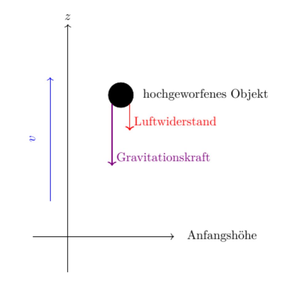
Wie lautet die Bewegungsgleichung? (Hinweis: \(F = m \cdot a\).)
- \(\frac{dv}{dt} - \frac{k}{m} v = -g\)
- \(\frac{dv}{dt} + \frac{k}{m} v = g\)
- \(-\frac{dv}{dt} + \frac{k}{m} v = -g\)
- \(\frac{dv}{dt} + \frac{k}{m} v = -g\)
Back
ETH::2._Semester::Analysis::6._Differentialgleichungen::1._Aufstellen::3._Mechanik ETH::2._Semester::Analysis::Serie::11
Ein Körper der Masse \(m\) wird mit Anfangsgeschwindigkeit \(v_0\) senkrecht in die Höhe geworfen. Der Luftwiderstand sei proportional zur Geschwindigkeit (positive Konstante \(k\)).
Wie lautet die Bewegungsgleichung? (Hinweis: \(F = m \cdot a\).)
- \(\frac{dv}{dt} - \frac{k}{m} v = -g\)
- \(\frac{dv}{dt} + \frac{k}{m} v = g\)
- \(-\frac{dv}{dt} + \frac{k}{m} v = -g\)
- \(\frac{dv}{dt} + \frac{k}{m} v = -g\)
(d) Mit \(F = m \tfrac{dv}{dt}\) und \(F = -mg - kv\) (beide Kräfte zeigen nach unten) folgt \(-mg - kv = m \tfrac{dv}{dt}\), also \(\tfrac{dv}{dt} + \tfrac{k}{m} v = -g\).
(a), (b), (c) haben falsche Vorzeichen bei den Kräfte-Richtungen.
Field-by-field Comparison
| Field |
Before |
After |
| Front |
|
Ein Körper der Masse \(m\) wird mit Anfangsgeschwindigkeit \(v_0\) senkrecht in die Höhe geworfen. Der Luftwiderstand sei proportional zur Geschwindigkeit (positive Konstante \(k\)).<br><br><img src="paste-bcde334cd6c1c6e9f90506909d928014e8c2bcd3.jpg"><br><br>Wie lautet die Bewegungsgleichung? (Hinweis: \(F = m \cdot a\).)<ol type="a"><li>\(\frac{dv}{dt} - \frac{k}{m} v = -g\)</li><li>\(\frac{dv}{dt} + \frac{k}{m} v = g\)</li><li>\(-\frac{dv}{dt} + \frac{k}{m} v = -g\)</li><li>\(\frac{dv}{dt} + \frac{k}{m} v = -g\)</li></ol> |
| Back |
|
<b>(d)</b> Mit \(F = m \tfrac{dv}{dt}\) und \(F = -mg - kv\) (beide Kräfte zeigen nach unten) folgt \(-mg - kv = m \tfrac{dv}{dt}\), also \(\tfrac{dv}{dt} + \tfrac{k}{m} v = -g\).<br><br>(a), (b), (c) haben falsche Vorzeichen bei den Kräfte-Richtungen. |
Tags:
ETH::2._Semester::Analysis::6._Differentialgleichungen::1._Aufstellen::3._Mechanik
ETH::2._Semester::Analysis::Serie::11
Note 70: ETH::2. Semester::Analysis
Deck: ETH::2. Semester::Analysis
Note Type: Horvath Cloze
GUID: D=5{vpKx'.
added
Previous
Note did not exist
New Note
Front
ETH::2._Semester::Analysis::6._Differentialgleichungen::3._Lösungstechniken_erster_Ordnung::0._Übersicht
Lösungstechniken für DifferentialgleichungenDGl
erster Ordnung:
- Trennung der Variablen
- Substitution
- Variation der Konstanten (lineare, inhomogene DGl)
Lineare, inhomogene DGl
beliebiger Ordnung:
- geeignete Ansätze für die partikuläre Lösung
Back
ETH::2._Semester::Analysis::6._Differentialgleichungen::3._Lösungstechniken_erster_Ordnung::0._Übersicht
Lösungstechniken für DifferentialgleichungenDGl
erster Ordnung:
- Trennung der Variablen
- Substitution
- Variation der Konstanten (lineare, inhomogene DGl)
Lineare, inhomogene DGl
beliebiger Ordnung:
- geeignete Ansätze für die partikuläre Lösung
Field-by-field Comparison
| Field |
Before |
After |
| Text |
|
<b>Lösungstechniken für Differentialgleichungen</b><br>DGl <b>erster Ordnung</b>:<ul><li>{{c1::Trennung der Variablen}}</li><li>{{c1::Substitution}}</li><li>{{c1::Variation der Konstanten}} (lineare, inhomogene DGl)</li></ul>Lineare, inhomogene DGl <b>beliebiger Ordnung</b>:<ul><li>{{c2::geeignete Ansätze für die partikuläre Lösung}}</li></ul> |
Tags:
ETH::2._Semester::Analysis::6._Differentialgleichungen::3._Lösungstechniken_erster_Ordnung::0._Übersicht
Note 71: ETH::2. Semester::Analysis
Deck: ETH::2. Semester::Analysis
Note Type: Horvath Cloze
GUID: E#P*nHH>$>
modified
Before
Front
ETH::2._Semester::Analysis::1._Logik,_Mengen,_Zahlen::3._Zahlen::4._Komplexe_Zahlen::4._Einheitswurzeln
Sei \(n \in \mathbb{N}\), \(n \ge 1\).
Dann hat die Gleichung \(z^n = 1\) genau \(n\) Lösungen in \(\mathbb{C}\): \(z_1, z_2, \dots, z_n\) wobei: \[ z_j = {{c1:: \cos \frac{2\pi j}{n} + i \cdot \sin \frac{2 \pi j}{n} }}, \quad 1 \le j \le n \]
Back
ETH::2._Semester::Analysis::1._Logik,_Mengen,_Zahlen::3._Zahlen::4._Komplexe_Zahlen::4._Einheitswurzeln
Sei \(n \in \mathbb{N}\), \(n \ge 1\).
Dann hat die Gleichung \(z^n = 1\) genau \(n\) Lösungen in \(\mathbb{C}\): \(z_1, z_2, \dots, z_n\) wobei: \[ z_j = {{c1:: \cos \frac{2\pi j}{n} + i \cdot \sin \frac{2 \pi j}{n} }}, \quad 1 \le j \le n \]
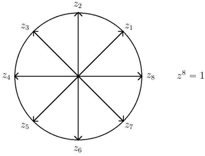
Die Lösungen liegen alle auf einem Kreis mit Radius 1 und sind gleichmäßig verteilt (formen ein n-Eck).
Beispiel:
Für \(w = R \cdot e^{i \varphi}\) sind die Lösungen von \(z^n = w\) gleich der \(n\) komplexen Zahlen mit Betrag \(\sqrt[^n]{R}\) und Winkeln \(\varphi_k = \frac{\varphi}{n} + k \cdot \frac{2 \pi}{n}\) für \(k = 0, \dots, n - 1\).
After
Front
ETH::2._Semester::Analysis::1._Logik,_Mengen,_Zahlen::3._Zahlen::4._Komplexe_Zahlen::4._Einheitswurzeln
Sei \(n \in \mathbb{N}\), \(n \ge 1\).
Dann hat die Gleichung \(z^n = 1\) genau \(n\) Lösungen in \(\mathbb{C}\): \(z_1, z_2, \dots, z_n\) wobei: \[ z_j = {{c1:: \cos \frac{2\pi j}{n} + i \cdot \sin \frac{2 \pi j}{n} }}, \quad 1 \le j \le n \]
Back
ETH::2._Semester::Analysis::1._Logik,_Mengen,_Zahlen::3._Zahlen::4._Komplexe_Zahlen::4._Einheitswurzeln
Sei \(n \in \mathbb{N}\), \(n \ge 1\).
Dann hat die Gleichung \(z^n = 1\) genau \(n\) Lösungen in \(\mathbb{C}\): \(z_1, z_2, \dots, z_n\) wobei: \[ z_j = {{c1:: \cos \frac{2\pi j}{n} + i \cdot \sin \frac{2 \pi j}{n} }}, \quad 1 \le j \le n \]
Die Lösungen liegen alle auf einem Kreis mit Radius 1 und sind gleichmässig verteilt (formen ein n-Eck).
Beispiel:
Für \(w = R \cdot e^{i \varphi}\) sind die Lösungen von \(z^n = w\) gleich der \(n\) komplexen Zahlen mit Betrag \(\sqrt[^n]{R}\) und Winkeln \(\varphi_k = \frac{\varphi}{n} + k \cdot \frac{2 \pi}{n}\) für \(k = 0, \dots, n - 1\).
Field-by-field Comparison
| Field |
Before |
After |
| Extra |
<img src="paste-d82ffaf45ffbd9d16177968af1e2d0295676539b.jpg"><br><div>Die Lösungen liegen alle auf einem Kreis mit Radius 1 und sind gleichmäßig verteilt (formen ein n-Eck).</div><div><br></div> <div>Beispiel: </div><div>Für \(w = R \cdot e^{i \varphi}\) sind die Lösungen von \(z^n = w\) gleich der \(n\) komplexen Zahlen mit Betrag \(\sqrt[^n]{R}\) und Winkeln \(\varphi_k = \frac{\varphi}{n} + k \cdot \frac{2 \pi}{n}\) für \(k = 0, \dots, n - 1\).</div> |
<img src="paste-d82ffaf45ffbd9d16177968af1e2d0295676539b.jpg"><br><div>Die Lösungen liegen alle auf einem Kreis mit Radius 1 und sind gleichmässig verteilt (formen ein n-Eck).</div><div><br></div> <div>Beispiel: </div><div>Für \(w = R \cdot e^{i \varphi}\) sind die Lösungen von \(z^n = w\) gleich der \(n\) komplexen Zahlen mit Betrag \(\sqrt[^n]{R}\) und Winkeln \(\varphi_k = \frac{\varphi}{n} + k \cdot \frac{2 \pi}{n}\) für \(k = 0, \dots, n - 1\).</div> |
Tags:
ETH::2._Semester::Analysis::1._Logik,_Mengen,_Zahlen::3._Zahlen::4._Komplexe_Zahlen::4._Einheitswurzeln
Note 72: ETH::2. Semester::Analysis
Deck: ETH::2. Semester::Analysis
Note Type: Horvath Cloze
GUID: E64n;i5!9x
added
Previous
Note did not exist
New Note
Front
ETH::2._Semester::Analysis::6._Differentialgleichungen::4._Lineare_inhomogene::2._Variation_der_Konstanten
Variation der Konstanten (DGl erster Ordnung)
Einen Ansatz für die partikuläre Lösung einer inhomogenen, linearen DGl erhält man, indem man in der allgemeinen Lösung der dazugehörigen homogenen DGl die auftretende Konstante durch eine Funktion in der unabhängigen Variablen ersetzt.
Back
ETH::2._Semester::Analysis::6._Differentialgleichungen::4._Lineare_inhomogene::2._Variation_der_Konstanten
Variation der Konstanten (DGl erster Ordnung)
Einen Ansatz für die partikuläre Lösung einer inhomogenen, linearen DGl erhält man, indem man in der allgemeinen Lösung der dazugehörigen homogenen DGl die auftretende Konstante durch eine Funktion in der unabhängigen Variablen ersetzt.
Dieser Ansatz heisst Variation der Konstanten.
Field-by-field Comparison
| Field |
Before |
After |
| Text |
|
<b>Variation der Konstanten</b> (DGl erster Ordnung)<br>Einen Ansatz für die partikuläre Lösung einer inhomogenen, linearen DGl erhält man, indem man {{c1::in der allgemeinen Lösung der dazugehörigen homogenen DGl die auftretende Konstante durch eine Funktion in der unabhängigen Variablen ersetzt}}. |
| Extra |
|
Dieser Ansatz heisst <b>Variation der Konstanten</b>. |
Tags:
ETH::2._Semester::Analysis::6._Differentialgleichungen::4._Lineare_inhomogene::2._Variation_der_Konstanten
Note 73: ETH::2. Semester::Analysis
Deck: ETH::2. Semester::Analysis
Note Type: Horvath Cloze
GUID: F.4_b[[a[X
added
Previous
Note did not exist
New Note
Front
ETH::2._Semester::Analysis::6._Differentialgleichungen::4._Lineare_inhomogene::3._Ansatz_partikuläre_Lösung
Ansatz für die partikuläre Lösung bei einer exponentiellen Störfunktion
Störfunktion \(s(t) = A e^{kt}\):
\[ y(t) = {{c1::C e^{kt} }} \]Spezialfall (Resonanz): Ist \(k\) eine \(m\)-fache Nullstelle des charakteristischen Polynoms, so lautet der Ansatz
\[ y(t) = {{c2::(C e^{kt})\, t^m}} \]
Back
ETH::2._Semester::Analysis::6._Differentialgleichungen::4._Lineare_inhomogene::3._Ansatz_partikuläre_Lösung
Ansatz für die partikuläre Lösung bei einer exponentiellen Störfunktion
Störfunktion \(s(t) = A e^{kt}\):
\[ y(t) = {{c1::C e^{kt} }} \]Spezialfall (Resonanz): Ist \(k\) eine \(m\)-fache Nullstelle des charakteristischen Polynoms, so lautet der Ansatz
\[ y(t) = {{c2::(C e^{kt})\, t^m}} \]
Field-by-field Comparison
| Field |
Before |
After |
| Text |
|
<b>Ansatz für die partikuläre Lösung</b> bei einer <b>exponentiellen</b> Störfunktion<br>Störfunktion \(s(t) = A e^{kt}\):<br>\[ y(t) = {{c1::C e^{kt} }} \]<b>Spezialfall</b> (Resonanz): Ist \(k\) eine \(m\)-fache Nullstelle des charakteristischen Polynoms, so lautet der Ansatz<br>\[ y(t) = {{c2::(C e^{kt})\, t^m}} \] |
Tags:
ETH::2._Semester::Analysis::6._Differentialgleichungen::4._Lineare_inhomogene::3._Ansatz_partikuläre_Lösung
Note 74: ETH::2. Semester::Analysis
Deck: ETH::2. Semester::Analysis
Note Type: Horvath Cloze
GUID: FVZ$*)>ic6
added
Previous
Note did not exist
New Note
Front
ETH::2._Semester::Analysis::6._Differentialgleichungen::4._Lineare_inhomogene::2._Variation_der_Konstanten
Variation der Konstanten: Beispiel \(y' - y = x\)
Die homogene DGl \(y' - y = 0\) hat die allgemeine Lösung \(y_h(x) = K e^x\).
Der Ansatz für die partikuläre Lösung (Variation der Konstanten) lautet daher
\[ y_p(x) = K(x)\,e^x \]
Back
ETH::2._Semester::Analysis::6._Differentialgleichungen::4._Lineare_inhomogene::2._Variation_der_Konstanten
Variation der Konstanten: Beispiel \(y' - y = x\)
Die homogene DGl \(y' - y = 0\) hat die allgemeine Lösung \(y_h(x) = K e^x\).
Der Ansatz für die partikuläre Lösung (Variation der Konstanten) lautet daher
\[ y_p(x) = K(x)\,e^x \]
Die Konstante \(K\) wird durch die Funktion \(K(x)\) ersetzt.
Field-by-field Comparison
| Field |
Before |
After |
| Text |
|
<b>Variation der Konstanten: Beispiel</b> \(y' - y = x\)<br>Die homogene DGl \(y' - y = 0\) hat die allgemeine Lösung \(y_h(x) = {{c1::K e^x}}\).<br>Der Ansatz für die partikuläre Lösung (Variation der Konstanten) lautet daher<br>\[ y_p(x) = {{c2::K(x)\,e^x}} \] |
| Extra |
|
Die Konstante \(K\) wird durch die Funktion \(K(x)\) ersetzt. |
Tags:
ETH::2._Semester::Analysis::6._Differentialgleichungen::4._Lineare_inhomogene::2._Variation_der_Konstanten
Note 75: ETH::2. Semester::Analysis
Deck: ETH::2. Semester::Analysis
Note Type: Horvath Classic
GUID: H_hzhh3U*j
added
Previous
Note did not exist
New Note
Front
ETH::2._Semester::Analysis::4._Funktionen::4._Elementare_Funktionen::5._Trigonometrische ETH::2._Semester::Analysis::Serie::7
Die Funktion \(\tan x\) ist
- für alle reellen \(x\) stetig.
- für alle reellen \(x\) stetig, für die \(\tan x\) definiert ist.
- in \(x = \tfrac{\pi}{2} + k\pi\) nicht stetig, wobei \(k\) eine ganze Zahl ist.
Back
ETH::2._Semester::Analysis::4._Funktionen::4._Elementare_Funktionen::5._Trigonometrische ETH::2._Semester::Analysis::Serie::7
Die Funktion \(\tan x\) ist
- für alle reellen \(x\) stetig.
- für alle reellen \(x\) stetig, für die \(\tan x\) definiert ist.
- in \(x = \tfrac{\pi}{2} + k\pi\) nicht stetig, wobei \(k\) eine ganze Zahl ist.
(b) Da \(\sin x\) und \(\cos x\) stetig sind, ist auch \(\tan x = \tfrac{\sin x}{\cos x}\) stetig, wo es definiert ist, also für \(\cos x \neq 0\).
(a) ist falsch, da \(\tan x\) für \(x = \tfrac{\pi}{2} + k\pi\) nicht definiert ist. (c) ist falsch, da es an einer nicht definierten Stelle keinen Sinn macht, nach Stetigkeit zu fragen.
Field-by-field Comparison
| Field |
Before |
After |
| Front |
|
Die Funktion \(\tan x\) ist<ol type="a"><li>für alle reellen \(x\) stetig.</li><li>für alle reellen \(x\) stetig, für die \(\tan x\) definiert ist.</li><li>in \(x = \tfrac{\pi}{2} + k\pi\) nicht stetig, wobei \(k\) eine ganze Zahl ist.</li></ol> |
| Back |
|
<b>(b)</b> Da \(\sin x\) und \(\cos x\) stetig sind, ist auch \(\tan x = \tfrac{\sin x}{\cos x}\) stetig, wo es definiert ist, also für \(\cos x \neq 0\).<br><br>(a) ist falsch, da \(\tan x\) für \(x = \tfrac{\pi}{2} + k\pi\) nicht definiert ist. (c) ist falsch, da es an einer nicht definierten Stelle keinen Sinn macht, nach Stetigkeit zu fragen. |
Tags:
ETH::2._Semester::Analysis::4._Funktionen::4._Elementare_Funktionen::5._Trigonometrische
ETH::2._Semester::Analysis::Serie::7
Note 76: ETH::2. Semester::Analysis
Deck: ETH::2. Semester::Analysis
Note Type: Horvath Classic
GUID: Hyf27xb$Im
added
Previous
Note did not exist
New Note
Front
ETH::2._Semester::Analysis::6._Differentialgleichungen::2._Lineare_homogene::3._Eulerscher_Ansatz ETH::2._Semester::Analysis::Serie::11
Wir betrachten die Differentialgleichung \(u''(x) - 2u'(x) - 15u(x) = 0\). Welche der folgenden Funktionen ist eine Lösung?
- \(e^{-5x}\)
- \(3e^{5x} + 5e^{-3x}\)
- \(e^{5x} + xe^{5x}\)
- \(xe^{-3x}\)
Back
ETH::2._Semester::Analysis::6._Differentialgleichungen::2._Lineare_homogene::3._Eulerscher_Ansatz ETH::2._Semester::Analysis::Serie::11
Wir betrachten die Differentialgleichung \(u''(x) - 2u'(x) - 15u(x) = 0\). Welche der folgenden Funktionen ist eine Lösung?
- \(e^{-5x}\)
- \(3e^{5x} + 5e^{-3x}\)
- \(e^{5x} + xe^{5x}\)
- \(xe^{-3x}\)
(b) Das charakteristische Polynom \(\lambda^2 - 2\lambda - 15 = (\lambda - 5)(\lambda + 3)\) hat die Nullstellen \(5\) und \(-3\). Also sind \(e^{5x}\) und \(e^{-3x}\) Fundamentallösungen, und jede Linearkombination wie \(3e^{5x} + 5e^{-3x}\) löst die DGl.
(a), (c), (d) ergeben beim Einsetzen einen von null verschiedenen Term.
Field-by-field Comparison
| Field |
Before |
After |
| Front |
|
Wir betrachten die Differentialgleichung \(u''(x) - 2u'(x) - 15u(x) = 0\). Welche der folgenden Funktionen ist eine Lösung?<ol type="a"><li>\(e^{-5x}\)</li><li>\(3e^{5x} + 5e^{-3x}\)</li><li>\(e^{5x} + xe^{5x}\)</li><li>\(xe^{-3x}\)</li></ol> |
| Back |
|
<b>(b)</b> Das charakteristische Polynom \(\lambda^2 - 2\lambda - 15 = (\lambda - 5)(\lambda + 3)\) hat die Nullstellen \(5\) und \(-3\). Also sind \(e^{5x}\) und \(e^{-3x}\) Fundamentallösungen, und jede Linearkombination wie \(3e^{5x} + 5e^{-3x}\) löst die DGl.<br><br>(a), (c), (d) ergeben beim Einsetzen einen von null verschiedenen Term. |
Tags:
ETH::2._Semester::Analysis::6._Differentialgleichungen::2._Lineare_homogene::3._Eulerscher_Ansatz
ETH::2._Semester::Analysis::Serie::11
Note 77: ETH::2. Semester::Analysis
Deck: ETH::2. Semester::Analysis
Note Type: Horvath Classic
GUID: JqL;MmkJdC
added
Previous
Note did not exist
New Note
Front
ETH::2._Semester::Analysis::6._Differentialgleichungen::2._Lineare_homogene::1._Klassifizierung ETH::2._Semester::Analysis::Serie::11
Wir betrachten die Differentialgleichung \(u''(x) - e^x + e^u = 0\). Welche der folgenden Charakterisierungen ist korrekt?
- Es liegt eine homogene Differentialgleichung vor.
- Die Differentialgleichung ist nicht-linear.
- Die gegebene Differentialgleichung ist linear.
- Die gegebene Differentialgleichung kann mit Hilfe des Eulerschen Ansatzes gelöst werden.
Back
ETH::2._Semester::Analysis::6._Differentialgleichungen::2._Lineare_homogene::1._Klassifizierung ETH::2._Semester::Analysis::Serie::11
Wir betrachten die Differentialgleichung \(u''(x) - e^x + e^u = 0\). Welche der folgenden Charakterisierungen ist korrekt?
- Es liegt eine homogene Differentialgleichung vor.
- Die Differentialgleichung ist nicht-linear.
- Die gegebene Differentialgleichung ist linear.
- Die gegebene Differentialgleichung kann mit Hilfe des Eulerschen Ansatzes gelöst werden.
(b) Der Term \(e^u\) enthält die gesuchte Funktion nicht als erste Potenz, also liegt ein nicht-linearer Term in \(u\) vor.
(a) ist falsch (der Term \(e^x\) ist eine Inhomogenität). (c) ist falsch wegen \(e^u\). (d) ist falsch, da der Eulersche Ansatz lineare DGl mit konstanten Koeffizienten voraussetzt.
Field-by-field Comparison
| Field |
Before |
After |
| Front |
|
Wir betrachten die Differentialgleichung \(u''(x) - e^x + e^u = 0\). Welche der folgenden Charakterisierungen ist korrekt?<ol type="a"><li>Es liegt eine homogene Differentialgleichung vor.</li><li>Die Differentialgleichung ist nicht-linear.</li><li>Die gegebene Differentialgleichung ist linear.</li><li>Die gegebene Differentialgleichung kann mit Hilfe des Eulerschen Ansatzes gelöst werden.</li></ol> |
| Back |
|
<b>(b)</b> Der Term \(e^u\) enthält die gesuchte Funktion nicht als erste Potenz, also liegt ein nicht-linearer Term in \(u\) vor.<br><br>(a) ist falsch (der Term \(e^x\) ist eine Inhomogenität). (c) ist falsch wegen \(e^u\). (d) ist falsch, da der Eulersche Ansatz lineare DGl mit konstanten Koeffizienten voraussetzt. |
Tags:
ETH::2._Semester::Analysis::6._Differentialgleichungen::2._Lineare_homogene::1._Klassifizierung
ETH::2._Semester::Analysis::Serie::11
Note 78: ETH::2. Semester::Analysis
Deck: ETH::2. Semester::Analysis
Note Type: Horvath Cloze
GUID: KV/9VcWRp^
added
Previous
Note did not exist
New Note
Front
ETH::2._Semester::Analysis::6._Differentialgleichungen::4._Lineare_inhomogene::3._Ansatz_partikuläre_Lösung
Wahl des Ansatzes für die partikuläre Lösung (nach Typ der Störfunktion):
- Störfunktion ist ein Polynom \(n\)-ten Grades \(\Rightarrow\) Ansatz: ein Polynom vom gleichen Grad
- Störfunktion ist eine Schwingung \(\Rightarrow\) Ansatz: eine Schwingung der gleichen Frequenz
- Störfunktion ist ein Produkt aus Polynom und Exponentialfunktion \(\Rightarrow\) Ansatz: ein Produkt aus einem Polynom gleichen Grades und einer Exponentialfunktion mit gleichem Exponenten
Back
ETH::2._Semester::Analysis::6._Differentialgleichungen::4._Lineare_inhomogene::3._Ansatz_partikuläre_Lösung
Wahl des Ansatzes für die partikuläre Lösung (nach Typ der Störfunktion):
- Störfunktion ist ein Polynom \(n\)-ten Grades \(\Rightarrow\) Ansatz: ein Polynom vom gleichen Grad
- Störfunktion ist eine Schwingung \(\Rightarrow\) Ansatz: eine Schwingung der gleichen Frequenz
- Störfunktion ist ein Produkt aus Polynom und Exponentialfunktion \(\Rightarrow\) Ansatz: ein Produkt aus einem Polynom gleichen Grades und einer Exponentialfunktion mit gleichem Exponenten
Field-by-field Comparison
| Field |
Before |
After |
| Text |
|
<b>Wahl des Ansatzes für die partikuläre Lösung</b> (nach Typ der Störfunktion):<ul><li>Störfunktion ist ein <b>Polynom</b> \(n\)-ten Grades \(\Rightarrow\) Ansatz: {{c1::ein Polynom vom gleichen Grad}}</li><li>Störfunktion ist eine <b>Schwingung</b> \(\Rightarrow\) Ansatz: {{c2::eine Schwingung der gleichen Frequenz}}</li><li>Störfunktion ist ein <b>Produkt aus Polynom und Exponentialfunktion</b> \(\Rightarrow\) Ansatz: {{c3::ein Produkt aus einem Polynom gleichen Grades und einer Exponentialfunktion mit gleichem Exponenten}}</li></ul> |
Tags:
ETH::2._Semester::Analysis::6._Differentialgleichungen::4._Lineare_inhomogene::3._Ansatz_partikuläre_Lösung
Note 79: ETH::2. Semester::Analysis
Deck: ETH::2. Semester::Analysis
Note Type: Horvath Classic
GUID: Nf?cy!e&3$
added
Previous
Note did not exist
New Note
Front
ETH::2._Semester::Analysis::5._Differentialrechnung::6._Mittelwertsätze ETH::2._Semester::Analysis::Serie::9
Ein Wagen fährt auf einer Strecke und kommt nacheinander an den Punkten \(A\) und \(B\) vorbei. Beide Punkte passiert der Wagen mit einer Geschwindigkeit von \(60\) km/h. Daher gibt es zwischen \(A\) und \(B\) mindestens einen Ort, an dem der Wagen nicht beschleunigt wird. Wahr oder Falsch?
- Richtig.
- Falsch.
Back
ETH::2._Semester::Analysis::5._Differentialrechnung::6._Mittelwertsätze ETH::2._Semester::Analysis::Serie::9
Ein Wagen fährt auf einer Strecke und kommt nacheinander an den Punkten \(A\) und \(B\) vorbei. Beide Punkte passiert der Wagen mit einer Geschwindigkeit von \(60\) km/h. Daher gibt es zwischen \(A\) und \(B\) mindestens einen Ort, an dem der Wagen nicht beschleunigt wird. Wahr oder Falsch?
- Richtig.
- Falsch.
(a) Richtig. Unter der Voraussetzung einer stetig differenzierbaren Bewegung garantiert der Mittelwertsatz eine Stelle, an der die Beschleunigung gleich dem Quotienten aus Geschwindigkeitsdifferenz und verstrichener Zeit ist. Da die Geschwindigkeiten bei \(A\) und \(B\) gleich sind, ist diese Differenz null, also existiert ein Punkt mit Beschleunigung null.
Field-by-field Comparison
| Field |
Before |
After |
| Front |
|
Ein Wagen fährt auf einer Strecke und kommt nacheinander an den Punkten \(A\) und \(B\) vorbei. Beide Punkte passiert der Wagen mit einer Geschwindigkeit von \(60\) km/h. Daher gibt es zwischen \(A\) und \(B\) mindestens einen Ort, an dem der Wagen nicht beschleunigt wird. Wahr oder Falsch?<ol type="a"><li>Richtig.</li><li>Falsch.</li></ol> |
| Back |
|
<b>(a)</b> Richtig. Unter der Voraussetzung einer stetig differenzierbaren Bewegung garantiert der Mittelwertsatz eine Stelle, an der die Beschleunigung gleich dem Quotienten aus Geschwindigkeitsdifferenz und verstrichener Zeit ist. Da die Geschwindigkeiten bei \(A\) und \(B\) gleich sind, ist diese Differenz null, also existiert ein Punkt mit Beschleunigung null. |
Tags:
ETH::2._Semester::Analysis::5._Differentialrechnung::6._Mittelwertsätze
ETH::2._Semester::Analysis::Serie::9
Note 80: ETH::2. Semester::Analysis
Deck: ETH::2. Semester::Analysis
Note Type: Horvath Classic
GUID: P/3L>A/cu(
added
Previous
Note did not exist
New Note
Front
ETH::2._Semester::Analysis::5._Differentialrechnung::6._Mittelwertsätze ETH::2._Semester::Analysis::Serie::9
Sei \(f : D \rightarrow \mathbb{R}\) differenzierbar, wobei \(D \subset \mathbb{R}\). Kreuze die richtigen Aussagen an.
- \(f\) ist stetig.
- \(f'\) ist stetig.
- Falls \(f'(x) = 0\) für alle \(x \in D\) gilt, dann existiert ein \(c \in \mathbb{R}\), so dass \(f(x) = c\) für alle \(x \in D\).
- Falls \(D = (a, b)\) mit \(a < b\) reelle Zahlen ist und \(f'(x) = 0\) für alle \(x \in D\) gilt, dann existiert ein \(c \in \mathbb{R}\) mit \(f(x) = c\) für alle \(x \in D\).
Back
ETH::2._Semester::Analysis::5._Differentialrechnung::6._Mittelwertsätze ETH::2._Semester::Analysis::Serie::9
Sei \(f : D \rightarrow \mathbb{R}\) differenzierbar, wobei \(D \subset \mathbb{R}\). Kreuze die richtigen Aussagen an.
- \(f\) ist stetig.
- \(f'\) ist stetig.
- Falls \(f'(x) = 0\) für alle \(x \in D\) gilt, dann existiert ein \(c \in \mathbb{R}\), so dass \(f(x) = c\) für alle \(x \in D\).
- Falls \(D = (a, b)\) mit \(a < b\) reelle Zahlen ist und \(f'(x) = 0\) für alle \(x \in D\) gilt, dann existiert ein \(c \in \mathbb{R}\) mit \(f(x) = c\) für alle \(x \in D\).
(a) und (d) sind richtig.
(a) Differenzierbarkeit impliziert Stetigkeit. (d) Auf einem Intervall folgt aus \(f' = 0\) mit dem Mittelwertsatz, dass \(f\) konstant ist.
(b) ist falsch: es gibt differenzierbare Funktionen mit unstetiger Ableitung. (c) ist falsch, wenn \(D\) nicht zusammenhängend ist (verschiedene konstante Werte auf verschiedenen Komponenten).
Field-by-field Comparison
| Field |
Before |
After |
| Front |
|
Sei \(f : D \rightarrow \mathbb{R}\) differenzierbar, wobei \(D \subset \mathbb{R}\). Kreuze die richtigen Aussagen an.<ol type="a"><li>\(f\) ist stetig.</li><li>\(f'\) ist stetig.</li><li>Falls \(f'(x) = 0\) für alle \(x \in D\) gilt, dann existiert ein \(c \in \mathbb{R}\), so dass \(f(x) = c\) für alle \(x \in D\).</li><li>Falls \(D = (a, b)\) mit \(a < b\) reelle Zahlen ist und \(f'(x) = 0\) für alle \(x \in D\) gilt, dann existiert ein \(c \in \mathbb{R}\) mit \(f(x) = c\) für alle \(x \in D\).</li></ol> |
| Back |
|
<b>(a) und (d)</b> sind richtig.<br><br>(a) Differenzierbarkeit impliziert Stetigkeit. (d) Auf einem Intervall folgt aus \(f' = 0\) mit dem Mittelwertsatz, dass \(f\) konstant ist.<br><br>(b) ist falsch: es gibt differenzierbare Funktionen mit unstetiger Ableitung. (c) ist falsch, wenn \(D\) nicht zusammenhängend ist (verschiedene konstante Werte auf verschiedenen Komponenten). |
Tags:
ETH::2._Semester::Analysis::5._Differentialrechnung::6._Mittelwertsätze
ETH::2._Semester::Analysis::Serie::9
Note 81: ETH::2. Semester::Analysis
Deck: ETH::2. Semester::Analysis
Note Type: Horvath Classic
GUID: P/3ktD{)S3
added
Previous
Note did not exist
New Note
Front
ETH::2._Semester::Analysis::6._Differentialgleichungen::2._Lineare_homogene::2._Lösungsstruktur ETH::2._Semester::Analysis::Serie::11
Es geht um die lineare DGl \(u^{(n)} + a_{n-1} u^{(n-1)} + \dots + a_1 u' + a_0 u = b\) (L) mit Inhomogenität \(b \neq 0\) und die zugehörige homogene Gleichung (H). Entscheiden Sie: Sind \(u_1\) und \(u_2\) Lösungen von (L), so ist \(u_1 - u_2\) auch eine Lösung von (L).
- Richtig.
- Falsch.
Back
ETH::2._Semester::Analysis::6._Differentialgleichungen::2._Lineare_homogene::2._Lösungsstruktur ETH::2._Semester::Analysis::Serie::11
Es geht um die lineare DGl \(u^{(n)} + a_{n-1} u^{(n-1)} + \dots + a_1 u' + a_0 u = b\) (L) mit Inhomogenität \(b \neq 0\) und die zugehörige homogene Gleichung (H). Entscheiden Sie: Sind \(u_1\) und \(u_2\) Lösungen von (L), so ist \(u_1 - u_2\) auch eine Lösung von (L).
- Richtig.
- Falsch.
(b) Falsch. Setzt man \(v = u_1 - u_2\) in den Differentialoperator ein, ergibt sich \(b - b = 0\), also löst \(v\) die homogene Gleichung (H). Da \(b \neq 0\), ist \(v\) somit gerade keine Lösung von (L).
Field-by-field Comparison
| Field |
Before |
After |
| Front |
|
Es geht um die lineare DGl \(u^{(n)} + a_{n-1} u^{(n-1)} + \dots + a_1 u' + a_0 u = b\) (L) mit Inhomogenität \(b \neq 0\) und die zugehörige homogene Gleichung (H). Entscheiden Sie: Sind \(u_1\) und \(u_2\) Lösungen von (L), so ist \(u_1 - u_2\) auch eine Lösung von (L).<ol type="a"><li>Richtig.</li><li>Falsch.</li></ol> |
| Back |
|
<b>(b)</b> Falsch. Setzt man \(v = u_1 - u_2\) in den Differentialoperator ein, ergibt sich \(b - b = 0\), also löst \(v\) die homogene Gleichung (H). Da \(b \neq 0\), ist \(v\) somit gerade keine Lösung von (L). |
Tags:
ETH::2._Semester::Analysis::6._Differentialgleichungen::2._Lineare_homogene::2._Lösungsstruktur
ETH::2._Semester::Analysis::Serie::11
Note 82: ETH::2. Semester::Analysis
Deck: ETH::2. Semester::Analysis
Note Type: Horvath Classic
GUID: S_fc1
added
Previous
Note did not exist
New Note
Front
ETH::2._Semester::Analysis::5._Differentialrechnung::9._Taylor::4._Rechenregeln ETH::2._Semester::Analysis::Serie::10
Bestimmen Sie \(\int_0^{1/2} \frac{\ln(1 + x)}{x}\, dx\) auf zwei Dezimalstellen genau.
- \(\frac{7}{16} \approx 0.43\)
- \(\frac{65}{144} \approx 0.45\)
- \(0.5\)
- Das Integral wird unendlich gross, da der Integrand einen Faktor \(\frac{1}{x}\) enthält.
Back
ETH::2._Semester::Analysis::5._Differentialrechnung::9._Taylor::4._Rechenregeln ETH::2._Semester::Analysis::Serie::10
Bestimmen Sie \(\int_0^{1/2} \frac{\ln(1 + x)}{x}\, dx\) auf zwei Dezimalstellen genau.
- \(\frac{7}{16} \approx 0.43\)
- \(\frac{65}{144} \approx 0.45\)
- \(0.5\)
- Das Integral wird unendlich gross, da der Integrand einen Faktor \(\frac{1}{x}\) enthält.
(b) Für \(|x| < 1\) gilt \(\tfrac{\ln(1+x)}{x} = \sum_{n=1}^{\infty} (-1)^{n+1} \tfrac{x^{n-1}}{n}\). Gliedweise Integration ergibt \(\sum_{n=1}^{\infty} \tfrac{(-1)^{n+1}}{n^2 2^n}\). Für zwei Dezimalstellen genügen die Terme bis \(n = 3\): \(\tfrac{1}{2} - \tfrac{1}{16} + \tfrac{1}{72} = \tfrac{65}{144} \approx 0.45\).
(d) ist falsch, da \(\lim_{x \to 0} \tfrac{\ln(1+x)}{x} = 1\) (l'Hospital), der Integrand also beschränkt bleibt.
Field-by-field Comparison
| Field |
Before |
After |
| Front |
|
Bestimmen Sie \(\int_0^{1/2} \frac{\ln(1 + x)}{x}\, dx\) auf zwei Dezimalstellen genau.<ol type="a"><li>\(\frac{7}{16} \approx 0.43\)</li><li>\(\frac{65}{144} \approx 0.45\)</li><li>\(0.5\)</li><li>Das Integral wird unendlich gross, da der Integrand einen Faktor \(\frac{1}{x}\) enthält.</li></ol> |
| Back |
|
<b>(b)</b> Für \(|x| < 1\) gilt \(\tfrac{\ln(1+x)}{x} = \sum_{n=1}^{\infty} (-1)^{n+1} \tfrac{x^{n-1}}{n}\). Gliedweise Integration ergibt \(\sum_{n=1}^{\infty} \tfrac{(-1)^{n+1}}{n^2 2^n}\). Für zwei Dezimalstellen genügen die Terme bis \(n = 3\): \(\tfrac{1}{2} - \tfrac{1}{16} + \tfrac{1}{72} = \tfrac{65}{144} \approx 0.45\).<br><br>(d) ist falsch, da \(\lim_{x \to 0} \tfrac{\ln(1+x)}{x} = 1\) (l'Hospital), der Integrand also beschränkt bleibt. |
Tags:
ETH::2._Semester::Analysis::5._Differentialrechnung::9._Taylor::4._Rechenregeln
ETH::2._Semester::Analysis::Serie::10
Note 83: ETH::2. Semester::Analysis
Deck: ETH::2. Semester::Analysis
Note Type: Horvath Classic
GUID: T7Ev@|DM%!
added
Previous
Note did not exist
New Note
Front
ETH::2._Semester::Analysis::5._Differentialrechnung::8._Monotonie_und_Konvexität ETH::2._Semester::Analysis::Serie::9
Sei \(f : (a, b) \rightarrow \mathbb{R}\) differenzierbar mit \(f'(t) > 0\) für alle \(t \in (a, b)\). Kreuze die richtige Aussage an.
- \(f\) ist positiv.
- \(f(x) < f(y)\) für alle \(x, y \in (a, b)\) mit \(x > y\).
- \(f(x) < f(y)\) für alle \(x, y \in (a, b)\) mit \(x \geq y\).
- \(f(x) < f(y)\) für alle \(x, y \in (a, b)\) mit \(x < y\).
Back
ETH::2._Semester::Analysis::5._Differentialrechnung::8._Monotonie_und_Konvexität ETH::2._Semester::Analysis::Serie::9
Sei \(f : (a, b) \rightarrow \mathbb{R}\) differenzierbar mit \(f'(t) > 0\) für alle \(t \in (a, b)\). Kreuze die richtige Aussage an.
- \(f\) ist positiv.
- \(f(x) < f(y)\) für alle \(x, y \in (a, b)\) mit \(x > y\).
- \(f(x) < f(y)\) für alle \(x, y \in (a, b)\) mit \(x \geq y\).
- \(f(x) < f(y)\) für alle \(x, y \in (a, b)\) mit \(x < y\).
(d) Nach dem Mittelwertsatz gibt es für \(x < y\) ein \(\xi \in (x, y)\) mit \(f(y) - f(x) = f'(\xi)(y - x) > 0\), also \(f(x) < f(y)\).
(a) ist falsch (\(f(x) = x\) wird negativ). (b) hat die Ungleichung verkehrt herum. (c) ist falsch, da für \(x = y\) Gleichheit gilt.
Field-by-field Comparison
| Field |
Before |
After |
| Front |
|
Sei \(f : (a, b) \rightarrow \mathbb{R}\) differenzierbar mit \(f'(t) > 0\) für alle \(t \in (a, b)\). Kreuze die richtige Aussage an.<ol type="a"><li>\(f\) ist positiv.</li><li>\(f(x) < f(y)\) für alle \(x, y \in (a, b)\) mit \(x > y\).</li><li>\(f(x) < f(y)\) für alle \(x, y \in (a, b)\) mit \(x \geq y\).</li><li>\(f(x) < f(y)\) für alle \(x, y \in (a, b)\) mit \(x < y\).</li></ol> |
| Back |
|
<b>(d)</b> Nach dem Mittelwertsatz gibt es für \(x < y\) ein \(\xi \in (x, y)\) mit \(f(y) - f(x) = f'(\xi)(y - x) > 0\), also \(f(x) < f(y)\).<br><br>(a) ist falsch (\(f(x) = x\) wird negativ). (b) hat die Ungleichung verkehrt herum. (c) ist falsch, da für \(x = y\) Gleichheit gilt. |
Tags:
ETH::2._Semester::Analysis::5._Differentialrechnung::8._Monotonie_und_Konvexität
ETH::2._Semester::Analysis::Serie::9
Note 84: ETH::2. Semester::Analysis
Deck: ETH::2. Semester::Analysis
Note Type: Horvath Classic
GUID: U-zC;j0n`U
added
Previous
Note did not exist
New Note
Front
ETH::2._Semester::Analysis::6._Differentialgleichungen::2._Lineare_homogene::3._Eulerscher_Ansatz ETH::2._Semester::Analysis::Serie::11
Betrachten Sie die Differentialgleichung \(u''(x) + 4u'(x) + 4u(x) = 0\). Welche der folgenden Funktionen ist eine Lösung?
- \(x^2 e^{-x}\)
- \(2xe^{-2x}\)
- \(3e^{2x}\)
- \(e^{-2x} + xe^{-3x}\)
Back
ETH::2._Semester::Analysis::6._Differentialgleichungen::2._Lineare_homogene::3._Eulerscher_Ansatz ETH::2._Semester::Analysis::Serie::11
Betrachten Sie die Differentialgleichung \(u''(x) + 4u'(x) + 4u(x) = 0\). Welche der folgenden Funktionen ist eine Lösung?
- \(x^2 e^{-x}\)
- \(2xe^{-2x}\)
- \(3e^{2x}\)
- \(e^{-2x} + xe^{-3x}\)
(b) Das charakteristische Polynom \(\lambda^2 + 4\lambda + 4 = (\lambda + 2)^2\) hat die doppelte Nullstelle \(-2\). Fundamentallösungen sind \(e^{-2x}\) und \(xe^{-2x}\), also löst \(2xe^{-2x}\) die DGl.
(a), (c), (d) ergeben beim Einsetzen einen von null verschiedenen Term.
Field-by-field Comparison
| Field |
Before |
After |
| Front |
|
Betrachten Sie die Differentialgleichung \(u''(x) + 4u'(x) + 4u(x) = 0\). Welche der folgenden Funktionen ist eine Lösung?<ol type="a"><li>\(x^2 e^{-x}\)</li><li>\(2xe^{-2x}\)</li><li>\(3e^{2x}\)</li><li>\(e^{-2x} + xe^{-3x}\)</li></ol> |
| Back |
|
<b>(b)</b> Das charakteristische Polynom \(\lambda^2 + 4\lambda + 4 = (\lambda + 2)^2\) hat die doppelte Nullstelle \(-2\). Fundamentallösungen sind \(e^{-2x}\) und \(xe^{-2x}\), also löst \(2xe^{-2x}\) die DGl.<br><br>(a), (c), (d) ergeben beim Einsetzen einen von null verschiedenen Term. |
Tags:
ETH::2._Semester::Analysis::6._Differentialgleichungen::2._Lineare_homogene::3._Eulerscher_Ansatz
ETH::2._Semester::Analysis::Serie::11
Note 85: ETH::2. Semester::Analysis
Deck: ETH::2. Semester::Analysis
Note Type: Horvath Classic
GUID: U3Q{.(uLY=
added
Previous
Note did not exist
New Note
Front
ETH::2._Semester::Analysis::6._Differentialgleichungen::2._Lineare_homogene::2._Lösungsstruktur ETH::2._Semester::Analysis::Serie::11
Welche Aussage trifft im Zusammenhang mit dem Anfangswertproblem \(y'(t) = f(y(t))\), \(y(0) = 0\) zu, wobei \(f(u) = -1\) für \(u \geq 0\) und \(f(u) = 1\) für \(u < 0\)?
- \(y'(0) = -1\).
- \(y(3) = -3\).
- \(\lim_{x \to \infty} y(x) = -\infty\).
- Das Problem hat keine Lösung, d.h. es existiert keine differenzierbare Funktion, welche das gegebene Problem löst.
Back
ETH::2._Semester::Analysis::6._Differentialgleichungen::2._Lineare_homogene::2._Lösungsstruktur ETH::2._Semester::Analysis::Serie::11
Welche Aussage trifft im Zusammenhang mit dem Anfangswertproblem \(y'(t) = f(y(t))\), \(y(0) = 0\) zu, wobei \(f(u) = -1\) für \(u \geq 0\) und \(f(u) = 1\) für \(u < 0\)?
- \(y'(0) = -1\).
- \(y(3) = -3\).
- \(\lim_{x \to \infty} y(x) = -\infty\).
- Das Problem hat keine Lösung, d.h. es existiert keine differenzierbare Funktion, welche das gegebene Problem löst.
(d) Das Problem hat keine Lösung. Es gibt kein \(\varepsilon > 0\) und keine stetige Funktion \(y : [0, \varepsilon) \rightarrow \mathbb{R}\), sodass \(y'(x) = f(y(x))\) für alle \(x \in (0, \varepsilon)\) gilt, da die rechte Seite bei \(y = 0\) widersprüchliche Steigungen erzwingt.
Field-by-field Comparison
| Field |
Before |
After |
| Front |
|
Welche Aussage trifft im Zusammenhang mit dem Anfangswertproblem \(y'(t) = f(y(t))\), \(y(0) = 0\) zu, wobei \(f(u) = -1\) für \(u \geq 0\) und \(f(u) = 1\) für \(u < 0\)?<ol type="a"><li>\(y'(0) = -1\).</li><li>\(y(3) = -3\).</li><li>\(\lim_{x \to \infty} y(x) = -\infty\).</li><li>Das Problem hat keine Lösung, d.h. es existiert keine differenzierbare Funktion, welche das gegebene Problem löst.</li></ol> |
| Back |
|
<b>(d)</b> Das Problem hat keine Lösung. Es gibt kein \(\varepsilon > 0\) und keine stetige Funktion \(y : [0, \varepsilon) \rightarrow \mathbb{R}\), sodass \(y'(x) = f(y(x))\) für alle \(x \in (0, \varepsilon)\) gilt, da die rechte Seite bei \(y = 0\) widersprüchliche Steigungen erzwingt. |
Tags:
ETH::2._Semester::Analysis::6._Differentialgleichungen::2._Lineare_homogene::2._Lösungsstruktur
ETH::2._Semester::Analysis::Serie::11
Note 86: ETH::2. Semester::Analysis
Deck: ETH::2. Semester::Analysis
Note Type: Horvath Classic
GUID: _:-R2ABQ3+
added
Previous
Note did not exist
New Note
Front
ETH::2._Semester::Analysis::4._Funktionen::2._Properties ETH::2._Semester::Analysis::Serie::7
Seien \(f, g : D \rightarrow \mathbb{R}\) monoton wachsende Funktionen, \(D \subseteq \mathbb{R}\). Wählen Sie die einzige richtige Antwort.
- \(f \cdot g : D \rightarrow \mathbb{R}\) ist monoton wachsend.
- Angenommen \(g(x) \neq 0\) für alle \(x \in D\). Dann ist \(\tfrac{f}{g}\) monoton wachsend.
- Angenommen \(f(x), g(x) \neq 0\) für alle \(x \in D\). Dann ist \(\tfrac{f}{g}\) oder \(\tfrac{g}{f}\) monoton wachsend.
- Alle obigen Aussagen sind falsch.
Back
ETH::2._Semester::Analysis::4._Funktionen::2._Properties ETH::2._Semester::Analysis::Serie::7
Seien \(f, g : D \rightarrow \mathbb{R}\) monoton wachsende Funktionen, \(D \subseteq \mathbb{R}\). Wählen Sie die einzige richtige Antwort.
- \(f \cdot g : D \rightarrow \mathbb{R}\) ist monoton wachsend.
- Angenommen \(g(x) \neq 0\) für alle \(x \in D\). Dann ist \(\tfrac{f}{g}\) monoton wachsend.
- Angenommen \(f(x), g(x) \neq 0\) für alle \(x \in D\). Dann ist \(\tfrac{f}{g}\) oder \(\tfrac{g}{f}\) monoton wachsend.
- Alle obigen Aussagen sind falsch.
(d) Alle obigen Aussagen sind falsch.
(a) Gegenbeispiel \(f(x) = g(x) = x\) auf \(D = \mathbb{R}\). (b) Gegenbeispiel \(D = (0, \infty)\), \(f(x) = x\), \(g(x) = x^2\), denn \(\tfrac{f}{g}(x) = \tfrac{1}{x}\) fällt. (c) Mit stückweise definierten \(f, g\) sind weder \(\tfrac{f}{g}\) noch \(\tfrac{g}{f}\) monoton.
Field-by-field Comparison
| Field |
Before |
After |
| Front |
|
Seien \(f, g : D \rightarrow \mathbb{R}\) monoton wachsende Funktionen, \(D \subseteq \mathbb{R}\). Wählen Sie die einzige richtige Antwort.<ol type="a"><li>\(f \cdot g : D \rightarrow \mathbb{R}\) ist monoton wachsend.</li><li>Angenommen \(g(x) \neq 0\) für alle \(x \in D\). Dann ist \(\tfrac{f}{g}\) monoton wachsend.</li><li>Angenommen \(f(x), g(x) \neq 0\) für alle \(x \in D\). Dann ist \(\tfrac{f}{g}\) oder \(\tfrac{g}{f}\) monoton wachsend.</li><li>Alle obigen Aussagen sind falsch.</li></ol> |
| Back |
|
<b>(d)</b> Alle obigen Aussagen sind falsch.<br><br>(a) Gegenbeispiel \(f(x) = g(x) = x\) auf \(D = \mathbb{R}\). (b) Gegenbeispiel \(D = (0, \infty)\), \(f(x) = x\), \(g(x) = x^2\), denn \(\tfrac{f}{g}(x) = \tfrac{1}{x}\) fällt. (c) Mit stückweise definierten \(f, g\) sind weder \(\tfrac{f}{g}\) noch \(\tfrac{g}{f}\) monoton. |
Tags:
ETH::2._Semester::Analysis::4._Funktionen::2._Properties
ETH::2._Semester::Analysis::Serie::7
Note 87: ETH::2. Semester::Analysis
Deck: ETH::2. Semester::Analysis
Note Type: Horvath Classic
GUID: _
added
Previous
Note did not exist
New Note
Front
ETH::2._Semester::Analysis::4._Funktionen::2._Properties ETH::2._Semester::Analysis::Serie::7
Sei \(f : D \rightarrow \mathbb{R}\) mit \(D \subseteq \mathbb{R}\).
Welche der folgenden Aussagen ist äquivalent zur Stetigkeit von \(f\)?
- Für alle \(x \in D\) und \(\varepsilon > 0\) existiert ein \(\delta > 0\), so dass für alle \(z \in D\) gilt: \(z \in (x - \delta, x + \delta) \Rightarrow f(z) \in (f(x) - \varepsilon, f(x) + \varepsilon)\).
- Für alle \(x \in D\) existiert ein \(\delta > 0\), so dass für alle \(\varepsilon > 0\) und \(z \in D\) gilt: \(|z - x| < \delta \Rightarrow |f(z) - f(x)| < \varepsilon\).
- Für alle \(\varepsilon > 0\) existiert \(\delta > 0\), so dass für alle \(x, z \in D\) gilt: \(|x - z| < \delta \Rightarrow |f(x) - f(z)| < \varepsilon\).
- Alle obigen Definitionen sind falsch.
Back
ETH::2._Semester::Analysis::4._Funktionen::2._Properties ETH::2._Semester::Analysis::Serie::7
Sei \(f : D \rightarrow \mathbb{R}\) mit \(D \subseteq \mathbb{R}\).
Welche der folgenden Aussagen ist äquivalent zur Stetigkeit von \(f\)?
- Für alle \(x \in D\) und \(\varepsilon > 0\) existiert ein \(\delta > 0\), so dass für alle \(z \in D\) gilt: \(z \in (x - \delta, x + \delta) \Rightarrow f(z) \in (f(x) - \varepsilon, f(x) + \varepsilon)\).
- Für alle \(x \in D\) existiert ein \(\delta > 0\), so dass für alle \(\varepsilon > 0\) und \(z \in D\) gilt: \(|z - x| < \delta \Rightarrow |f(z) - f(x)| < \varepsilon\).
- Für alle \(\varepsilon > 0\) existiert \(\delta > 0\), so dass für alle \(x, z \in D\) gilt: \(|x - z| < \delta \Rightarrow |f(x) - f(z)| < \varepsilon\).
- Alle obigen Definitionen sind falsch.
(a) Das ist genau die Stetigkeitsdefinition aus der Vorlesung, nur in Intervallschreibweise.
(b) ist falsch, weil die Quantoren in der falschen Reihenfolge stehen. (c) ist echt stärker als Stetigkeit (das \(\delta\) gilt gleichzeitig für alle \(x\)) und beschreibt die gleichmässige Stetigkeit.
Field-by-field Comparison
| Field |
Before |
After |
| Front |
|
Sei \(f : D \rightarrow \mathbb{R}\) mit \(D \subseteq \mathbb{R}\). <br>Welche der folgenden Aussagen ist äquivalent zur Stetigkeit von \(f\)?<ol type="a"><li>Für alle \(x \in D\) und \(\varepsilon > 0\) existiert ein \(\delta > 0\), so dass für alle \(z \in D\) gilt: \(z \in (x - \delta, x + \delta) \Rightarrow f(z) \in (f(x) - \varepsilon, f(x) + \varepsilon)\).</li><li>Für alle \(x \in D\) existiert ein \(\delta > 0\), so dass für alle \(\varepsilon > 0\) und \(z \in D\) gilt: \(|z - x| < \delta \Rightarrow |f(z) - f(x)| < \varepsilon\).</li><li>Für alle \(\varepsilon > 0\) existiert \(\delta > 0\), so dass für alle \(x, z \in D\) gilt: \(|x - z| < \delta \Rightarrow |f(x) - f(z)| < \varepsilon\).</li><li>Alle obigen Definitionen sind falsch.</li></ol> |
| Back |
|
<b>(a)</b> Das ist genau die Stetigkeitsdefinition aus der Vorlesung, nur in Intervallschreibweise.<br><br>(b) ist falsch, weil die Quantoren in der falschen Reihenfolge stehen. (c) ist echt stärker als Stetigkeit (das \(\delta\) gilt gleichzeitig für alle \(x\)) und beschreibt die <i>gleichmässige</i> Stetigkeit. |
Tags:
ETH::2._Semester::Analysis::4._Funktionen::2._Properties
ETH::2._Semester::Analysis::Serie::7
Note 88: ETH::2. Semester::Analysis
Deck: ETH::2. Semester::Analysis
Note Type: Horvath Classic
GUID: _qA35,18^@
added
Previous
Note did not exist
New Note
Front
ETH::2._Semester::Analysis::4._Funktionen::2._Properties ETH::2._Semester::Analysis::Serie::9
Definiere für \(x > 0\): \(f(x) := \liminf_{k \to \infty} \big(\min\{x, x^{-1}\}\big)^k\).
Welche Aussage gilt dann?
- \(f\) ist stetig und differenzierbar.
- \(f\) ist differenzierbar, aber nicht stetig.
- \(f\) ist stetig, aber nicht differenzierbar.
- \(f\) ist nicht stetig und nicht differenzierbar.
Back
ETH::2._Semester::Analysis::4._Funktionen::2._Properties ETH::2._Semester::Analysis::Serie::9
Definiere für \(x > 0\): \(f(x) := \liminf_{k \to \infty} \big(\min\{x, x^{-1}\}\big)^k\).
Welche Aussage gilt dann?
- \(f\) ist stetig und differenzierbar.
- \(f\) ist differenzierbar, aber nicht stetig.
- \(f\) ist stetig, aber nicht differenzierbar.
- \(f\) ist nicht stetig und nicht differenzierbar.
(d) Für \(x \neq 1\) liegt \(\min\{x, x^{-1}\}\) in \((0, 1)\), also konvergieren die Potenzen gegen \(0\); für \(x = 1\) ist der Ausdruck stets \(1\). Somit \(f(x) = 0\) für \(x \neq 1\) und \(f(1) = 1\). Damit ist \(f\) in \(x = 1\) unstetig und folglich dort auch nicht differenzierbar.
(a), (b), (c) scheitern alle an der Unstetigkeit in \(x = 1\); insbesondere impliziert Differenzierbarkeit Stetigkeit.
Field-by-field Comparison
| Field |
Before |
After |
| Front |
|
Definiere für \(x > 0\): \(f(x) := \liminf_{k \to \infty} \big(\min\{x, x^{-1}\}\big)^k\). <br>Welche Aussage gilt dann?<ol type="a"><li>\(f\) ist stetig und differenzierbar.</li><li>\(f\) ist differenzierbar, aber nicht stetig.</li><li>\(f\) ist stetig, aber nicht differenzierbar.</li><li>\(f\) ist nicht stetig und nicht differenzierbar.</li></ol> |
| Back |
|
<b>(d)</b> Für \(x \neq 1\) liegt \(\min\{x, x^{-1}\}\) in \((0, 1)\), also konvergieren die Potenzen gegen \(0\); für \(x = 1\) ist der Ausdruck stets \(1\). Somit \(f(x) = 0\) für \(x \neq 1\) und \(f(1) = 1\). Damit ist \(f\) in \(x = 1\) unstetig und folglich dort auch nicht differenzierbar.<br><br>(a), (b), (c) scheitern alle an der Unstetigkeit in \(x = 1\); insbesondere impliziert Differenzierbarkeit Stetigkeit. |
Tags:
ETH::2._Semester::Analysis::4._Funktionen::2._Properties
ETH::2._Semester::Analysis::Serie::9
Note 89: ETH::2. Semester::Analysis
Deck: ETH::2. Semester::Analysis
Note Type: Horvath Cloze
GUID: a(2w#VKag=
modified
Before
Front
ETH::2._Semester::Analysis::3._Reihen::3._Konvergenzkriterien
Seien \(a_n, b_n > 0\). Dann:
- {{c1::\(\lim \frac{a_n}{b_n} = g\) mit \(0 < g < \infty\)}} \(\implies\) \(\sum a_n\) und \(\sum b_n\) haben dasselbe Konvergenzverhalten
- {{c2::\(\lim \frac{a_n}{b_n} = 0\) und \(\sum b_n\) konvergiert}} \(\implies\) \(\sum a_n\) konvergiert
- {{c3::\(\lim \frac{a_n}{b_n} = \infty\) und \(\sum b_n\) divergiert }}\(\implies\) \(\sum a_n\) divergiert
Back
ETH::2._Semester::Analysis::3._Reihen::3._Konvergenzkriterien
Seien \(a_n, b_n > 0\). Dann:
- {{c1::\(\lim \frac{a_n}{b_n} = g\) mit \(0 < g < \infty\)}} \(\implies\) \(\sum a_n\) und \(\sum b_n\) haben dasselbe Konvergenzverhalten
- {{c2::\(\lim \frac{a_n}{b_n} = 0\) und \(\sum b_n\) konvergiert}} \(\implies\) \(\sum a_n\) konvergiert
- {{c3::\(\lim \frac{a_n}{b_n} = \infty\) und \(\sum b_n\) divergiert }}\(\implies\) \(\sum a_n\) divergiert
Grenzwertkriterium (Limitenvergleich)
Beispiel:\[\sum \frac{1}{n^2+3n}\]Vergleich mit \(1/n^2\), Grenzwert \(= 1\) → konvergiert.
Proof Sketch
- Ist \(\lim_{n \to \infty} \frac{a_n}{b_n} = g\) mit \(0 < g < \infty\)
- So gilt \(\frac{a_n}{b_n} \leq g + \varepsilon\) und daher \(a_n \leq (g + \varepsilon) \, b_n\) für ein geeignetes \(\varepsilon > 0\) und alle genügend großen \(n\).
- Nach dem Majorantenkriterium folgt aus der Konvergenz von \(\sum b_n\) die Konvergenz von \(\sum a_n\).
After
Front
ETH::2._Semester::Analysis::3._Reihen::3._Konvergenzkriterien
Seien \(a_n, b_n > 0\). Dann:
- {{c1::\(\lim \frac{a_n}{b_n} = g\) mit \(0 < g < \infty\)}} \(\implies\) \(\sum a_n\) und \(\sum b_n\) haben dasselbe Konvergenzverhalten
- {{c2::\(\lim \frac{a_n}{b_n} = 0\) und \(\sum b_n\) konvergiert}} \(\implies\) \(\sum a_n\) konvergiert
- {{c3::\(\lim \frac{a_n}{b_n} = \infty\) und \(\sum b_n\) divergiert }}\(\implies\) \(\sum a_n\) divergiert
Back
ETH::2._Semester::Analysis::3._Reihen::3._Konvergenzkriterien
Seien \(a_n, b_n > 0\). Dann:
- {{c1::\(\lim \frac{a_n}{b_n} = g\) mit \(0 < g < \infty\)}} \(\implies\) \(\sum a_n\) und \(\sum b_n\) haben dasselbe Konvergenzverhalten
- {{c2::\(\lim \frac{a_n}{b_n} = 0\) und \(\sum b_n\) konvergiert}} \(\implies\) \(\sum a_n\) konvergiert
- {{c3::\(\lim \frac{a_n}{b_n} = \infty\) und \(\sum b_n\) divergiert }}\(\implies\) \(\sum a_n\) divergiert
Grenzwertkriterium (Limitenvergleich)
Beispiel:\[\sum \frac{1}{n^2+3n}\]Vergleich mit \(1/n^2\), Grenzwert \(= 1\) → konvergiert.
Proof Sketch
- Ist \(\lim_{n \to \infty} \frac{a_n}{b_n} = g\) mit \(0 < g < \infty\)
- So gilt \(\frac{a_n}{b_n} \leq g + \varepsilon\) und daher \(a_n \leq (g + \varepsilon) \, b_n\) für ein geeignetes \(\varepsilon > 0\) und alle genügend grossen \(n\).
- Nach dem Majorantenkriterium folgt aus der Konvergenz von \(\sum b_n\) die Konvergenz von \(\sum a_n\).
Field-by-field Comparison
| Field |
Before |
After |
| Extra |
Grenzwertkriterium (Limitenvergleich)<b><br><br>Beispiel:</b>\[\sum \frac{1}{n^2+3n}\]Vergleich mit \(1/n^2\), Grenzwert \(= 1\) → konvergiert.<br><br><div><div><strong>Proof Sketch</strong></div>
<ul>
<li>Ist \(\lim_{n \to \infty} \frac{a_n}{b_n} = g\) mit \(0 < g < \infty\)</li>
<li>So gilt \(\frac{a_n}{b_n} \leq g + \varepsilon\) und daher \(a_n \leq (g + \varepsilon) \, b_n\) für ein geeignetes \(\varepsilon > 0\) und alle genügend großen \(n\). </li>
<li>Nach dem <em>Majorantenkriterium</em> folgt aus der Konvergenz von \(\sum b_n\) die Konvergenz von \(\sum a_n\).</li></ul></div> |
Grenzwertkriterium (Limitenvergleich)<b><br><br>Beispiel:</b>\[\sum \frac{1}{n^2+3n}\]Vergleich mit \(1/n^2\), Grenzwert \(= 1\) → konvergiert.<br><br><div><div><strong>Proof Sketch</strong></div>
<ul>
<li>Ist \(\lim_{n \to \infty} \frac{a_n}{b_n} = g\) mit \(0 < g < \infty\)</li>
<li>So gilt \(\frac{a_n}{b_n} \leq g + \varepsilon\) und daher \(a_n \leq (g + \varepsilon) \, b_n\) für ein geeignetes \(\varepsilon > 0\) und alle genügend grossen \(n\). </li>
<li>Nach dem <em>Majorantenkriterium</em> folgt aus der Konvergenz von \(\sum b_n\) die Konvergenz von \(\sum a_n\).</li></ul></div> |
Tags:
ETH::2._Semester::Analysis::3._Reihen::3._Konvergenzkriterien
Note 90: ETH::2. Semester::Analysis
Deck: ETH::2. Semester::Analysis
Note Type: Horvath Classic
GUID: a;(%@.PJ7`
added
Previous
Note did not exist
New Note
Front
ETH::2._Semester::Analysis::5._Differentialrechnung::5._Extremalstellen ETH::2._Semester::Analysis::Serie::10
Sei \(f : [-1, 1] \rightarrow \mathbb{R}\) eine glatte Funktion mit \(f(1/2) = 2\), \(f'(1/2) = 0\), \(f''(1/2) = -1\). Welche der folgenden Aussagen gilt?
- Die Funktion \(f\) besitzt ein lokales Maximum in \(1/2\).
- Die Funktion \(f\) besitzt ein lokales Minimum in \(1/2\).
- Die Funktion \(f\) besitzt kein lokales Extremum in \(1/2\).
- Alle oben genannten Fälle sind möglich.
Back
ETH::2._Semester::Analysis::5._Differentialrechnung::5._Extremalstellen ETH::2._Semester::Analysis::Serie::10
Sei \(f : [-1, 1] \rightarrow \mathbb{R}\) eine glatte Funktion mit \(f(1/2) = 2\), \(f'(1/2) = 0\), \(f''(1/2) = -1\). Welche der folgenden Aussagen gilt?
- Die Funktion \(f\) besitzt ein lokales Maximum in \(1/2\).
- Die Funktion \(f\) besitzt ein lokales Minimum in \(1/2\).
- Die Funktion \(f\) besitzt kein lokales Extremum in \(1/2\).
- Alle oben genannten Fälle sind möglich.
(a) Da \(f'(1/2) = 0\) und die zweite Ableitung dort negativ ist (mit gerader Ordnung \(2\)), besitzt \(f\) in \(1/2\) ein lokales Maximum.
Field-by-field Comparison
| Field |
Before |
After |
| Front |
|
Sei \(f : [-1, 1] \rightarrow \mathbb{R}\) eine glatte Funktion mit \(f(1/2) = 2\), \(f'(1/2) = 0\), \(f''(1/2) = -1\). Welche der folgenden Aussagen gilt?<ol type="a"><li>Die Funktion \(f\) besitzt ein lokales Maximum in \(1/2\).</li><li>Die Funktion \(f\) besitzt ein lokales Minimum in \(1/2\).</li><li>Die Funktion \(f\) besitzt kein lokales Extremum in \(1/2\).</li><li>Alle oben genannten Fälle sind möglich.</li></ol> |
| Back |
|
<b>(a)</b> Da \(f'(1/2) = 0\) und die zweite Ableitung dort negativ ist (mit gerader Ordnung \(2\)), besitzt \(f\) in \(1/2\) ein lokales Maximum. |
Tags:
ETH::2._Semester::Analysis::5._Differentialrechnung::5._Extremalstellen
ETH::2._Semester::Analysis::Serie::10
Note 91: ETH::2. Semester::Analysis
Deck: ETH::2. Semester::Analysis
Note Type: Horvath Classic
GUID: a]*J4hd?gS
added
Previous
Note did not exist
New Note
Front
ETH::2._Semester::Analysis::5._Differentialrechnung::4._Ableitungsregeln::2._Rechenregeln ETH::2._Semester::Analysis::Serie::8
Bestimmen Sie die Ableitung von \(\sqrt[4]{x^2 + 1}\).
- \(\frac{x}{2(x^2 + 1)^{3/4}}\)
- \(\frac{-4}{(x^2 + 1)^5}\)
- \(\frac{2x}{4\sqrt{x^2 + 1}}\)
- \(\sqrt[4]{x^2 + 1} \cdot 2x\)
Back
ETH::2._Semester::Analysis::5._Differentialrechnung::4._Ableitungsregeln::2._Rechenregeln ETH::2._Semester::Analysis::Serie::8
Bestimmen Sie die Ableitung von \(\sqrt[4]{x^2 + 1}\).
- \(\frac{x}{2(x^2 + 1)^{3/4}}\)
- \(\frac{-4}{(x^2 + 1)^5}\)
- \(\frac{2x}{4\sqrt{x^2 + 1}}\)
- \(\sqrt[4]{x^2 + 1} \cdot 2x\)
(a) Schreibe \((x^2 + 1)^{1/4}\). Ableiten ergibt \(\tfrac{1}{4}(x^2 + 1)^{-3/4} \cdot 2x = \tfrac{x}{2(x^2 + 1)^{3/4}}\).
(b) hat falsche Potenz und keine innere Ableitung. (c) hat Potenz \(-\tfrac{1}{2}\) statt \(-\tfrac{3}{4}\). (d) leitet die Wurzel falsch ab.
Field-by-field Comparison
| Field |
Before |
After |
| Front |
|
Bestimmen Sie die Ableitung von \(\sqrt[4]{x^2 + 1}\).<ol type="a"><li>\(\frac{x}{2(x^2 + 1)^{3/4}}\)</li><li>\(\frac{-4}{(x^2 + 1)^5}\)</li><li>\(\frac{2x}{4\sqrt{x^2 + 1}}\)</li><li>\(\sqrt[4]{x^2 + 1} \cdot 2x\)</li></ol> |
| Back |
|
<b>(a)</b> Schreibe \((x^2 + 1)^{1/4}\). Ableiten ergibt \(\tfrac{1}{4}(x^2 + 1)^{-3/4} \cdot 2x = \tfrac{x}{2(x^2 + 1)^{3/4}}\).<br><br>(b) hat falsche Potenz und keine innere Ableitung. (c) hat Potenz \(-\tfrac{1}{2}\) statt \(-\tfrac{3}{4}\). (d) leitet die Wurzel falsch ab. |
Tags:
ETH::2._Semester::Analysis::5._Differentialrechnung::4._Ableitungsregeln::2._Rechenregeln
ETH::2._Semester::Analysis::Serie::8
Note 92: ETH::2. Semester::Analysis
Deck: ETH::2. Semester::Analysis
Note Type: Horvath Classic
GUID: cB7
added
Previous
Note did not exist
New Note
Front
ETH::2._Semester::Analysis::5._Differentialrechnung::5._Extremalstellen ETH::2._Semester::Analysis::Serie::9
Sei \(f : [-1, 1] \rightarrow \mathbb{R}\) eine Funktion mit folgendem Graphen:
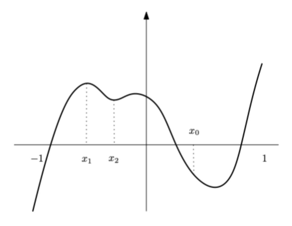
Welche der folgenden Aussagen gilt?
- Die Funktion \(f\) besitzt ein lokales Maximum in \(0\).
- \(f'(x_0) > 0\).
- \(f'(x_1) = 0\).
- \(f'(x_2) < 0\).
Back
ETH::2._Semester::Analysis::5._Differentialrechnung::5._Extremalstellen ETH::2._Semester::Analysis::Serie::9
Sei \(f : [-1, 1] \rightarrow \mathbb{R}\) eine Funktion mit folgendem Graphen:
Welche der folgenden Aussagen gilt?
- Die Funktion \(f\) besitzt ein lokales Maximum in \(0\).
- \(f'(x_0) > 0\).
- \(f'(x_1) = 0\).
- \(f'(x_2) < 0\).
(c) Am Punkt \(x_1\) besitzt der Graph eine waagrechte Tangente, also gilt \(f'(x_1) = 0\).
(a) ist falsch, da \(f(0)\) in keiner Umgebung von \(0\) grösster Funktionswert ist. (b) und (d) stimmen nicht mit den dargestellten Steigungen bei \(x_0\) bzw. \(x_2\) überein.
Field-by-field Comparison
| Field |
Before |
After |
| Front |
|
Sei \(f : [-1, 1] \rightarrow \mathbb{R}\) eine Funktion mit folgendem Graphen:<br><br><img src="paste-80876c83f7e621ab3e9b3cb0e10ee26b08f2f5ba.jpg"><br><br>Welche der folgenden Aussagen gilt?<ol type="a"><li>Die Funktion \(f\) besitzt ein lokales Maximum in \(0\).</li><li>\(f'(x_0) > 0\).</li><li>\(f'(x_1) = 0\).</li><li>\(f'(x_2) < 0\).</li></ol> |
| Back |
|
<b>(c)</b> Am Punkt \(x_1\) besitzt der Graph eine waagrechte Tangente, also gilt \(f'(x_1) = 0\).<br><br>(a) ist falsch, da \(f(0)\) in keiner Umgebung von \(0\) grösster Funktionswert ist. (b) und (d) stimmen nicht mit den dargestellten Steigungen bei \(x_0\) bzw. \(x_2\) überein. |
Tags:
ETH::2._Semester::Analysis::5._Differentialrechnung::5._Extremalstellen
ETH::2._Semester::Analysis::Serie::9
Note 93: ETH::2. Semester::Analysis
Deck: ETH::2. Semester::Analysis
Note Type: Horvath Cloze
GUID: cywhNH437V
added
Previous
Note did not exist
New Note
Front
ETH::2._Semester::Analysis::6._Differentialgleichungen::5._Existenz_und_Eindeutigkeit
Satz von Picard-Lindelöf-Peano (Ordnung \(n\))
Das Anfangswertproblem
\[ \begin{gathered} y^{(n)} + f_{n-1}(x) y^{(n-1)} + \dots + f_1(x) y' + f_0(x) y = s(x) \\ y(x_0) = y_0,\ y'(x_0) = v_0,\ \dots,\ y^{(n-1)}(x_0) = z_0 \end{gathered} \]besitzt für "vernünftige" Funktionen \(f_{n-1}, \dots, f_0, s\) eine eindeutige Lösung \(x \mapsto y(x)\), \(x \in I\),
wobei \(I\) von \(x_0\) und den gegebenen Anfangsdaten abhängen kann.
Back
ETH::2._Semester::Analysis::6._Differentialgleichungen::5._Existenz_und_Eindeutigkeit
Satz von Picard-Lindelöf-Peano (Ordnung \(n\))
Das Anfangswertproblem
\[ \begin{gathered} y^{(n)} + f_{n-1}(x) y^{(n-1)} + \dots + f_1(x) y' + f_0(x) y = s(x) \\ y(x_0) = y_0,\ y'(x_0) = v_0,\ \dots,\ y^{(n-1)}(x_0) = z_0 \end{gathered} \]besitzt für "vernünftige" Funktionen \(f_{n-1}, \dots, f_0, s\) eine eindeutige Lösung \(x \mapsto y(x)\), \(x \in I\),
wobei \(I\) von \(x_0\) und den gegebenen Anfangsdaten abhängen kann.
Field-by-field Comparison
| Field |
Before |
After |
| Text |
|
<b>Satz von Picard-Lindelöf-Peano (Ordnung \(n\))</b><br>Das Anfangswertproblem<br>\[ \begin{gathered} y^{(n)} + f_{n-1}(x) y^{(n-1)} + \dots + f_1(x) y' + f_0(x) y = s(x) \\ y(x_0) = y_0,\ y'(x_0) = v_0,\ \dots,\ y^{(n-1)}(x_0) = z_0 \end{gathered} \]besitzt für "vernünftige" Funktionen \(f_{n-1}, \dots, f_0, s\) {{c1::eine eindeutige Lösung}} \(x \mapsto y(x)\), \(x \in I\),<br>wobei \(I\) {{c2::von \(x_0\) und den gegebenen Anfangsdaten abhängen kann}}. |
Tags:
ETH::2._Semester::Analysis::6._Differentialgleichungen::5._Existenz_und_Eindeutigkeit
Note 94: ETH::2. Semester::Analysis
Deck: ETH::2. Semester::Analysis
Note Type: Horvath Cloze
GUID: e0d^/ml1oV
modified
Before
Front
ETH::2._Semester::Analysis::4._Funktionen::2._Properties
Der Graph einer Funktion heißt rechtsgekrümmt (Konkav) falls der Graph eine Rechtskurve vollführt / über der Sekante verläuft.
Back
ETH::2._Semester::Analysis::4._Funktionen::2._Properties
Der Graph einer Funktion heißt rechtsgekrümmt (Konkav) falls der Graph eine Rechtskurve vollführt / über der Sekante verläuft.
After
Front
ETH::2._Semester::Analysis::4._Funktionen::2._Properties
Der Graph einer Funktion heisst rechtsgekrümmt (Konkav) falls der Graph eine Rechtskurve vollführt / über der Sekante verläuft.
Back
ETH::2._Semester::Analysis::4._Funktionen::2._Properties
Der Graph einer Funktion heisst rechtsgekrümmt (Konkav) falls der Graph eine Rechtskurve vollführt / über der Sekante verläuft.
Field-by-field Comparison
| Field |
Before |
After |
| Text |
<div>Der Graph einer Funktion heißt {{c1::rechtsgekrümmt (Konkav)}} falls {{c2::der Graph eine Rechtskurve vollführt / über der Sekante verläuft}}.</div> |
<div>Der Graph einer Funktion heisst {{c1::rechtsgekrümmt (Konkav)}} falls {{c2::der Graph eine Rechtskurve vollführt / über der Sekante verläuft}}.</div> |
Tags:
ETH::2._Semester::Analysis::4._Funktionen::2._Properties
Note 95: ETH::2. Semester::Analysis
Deck: ETH::2. Semester::Analysis
Note Type: Horvath Cloze
GUID: euE$Yfzqg{
added
Previous
Note did not exist
New Note
Front
ETH::2._Semester::Analysis::6._Differentialgleichungen::3._Lösungstechniken_erster_Ordnung::2._Substitution
Nach der linearen Substitution \(u = ax + by + c\) erhält man aus \(y' = f(ax + by + c)\)
\[ \frac{du}{dx} = a + b\,f(u) \]Da hier die unabhängige Variable \(x\) nicht mehr explizit vorkommt, nennt man eine solche DGl autonom.
Back
ETH::2._Semester::Analysis::6._Differentialgleichungen::3._Lösungstechniken_erster_Ordnung::2._Substitution
Nach der linearen Substitution \(u = ax + by + c\) erhält man aus \(y' = f(ax + by + c)\)
\[ \frac{du}{dx} = a + b\,f(u) \]Da hier die unabhängige Variable \(x\) nicht mehr explizit vorkommt, nennt man eine solche DGl autonom.
Wegen \(\frac{du}{dx} = a + b\frac{dy}{dx} = a + b\,f(u)\).
Field-by-field Comparison
| Field |
Before |
After |
| Text |
|
Nach der linearen Substitution \(u = ax + by + c\) erhält man aus \(y' = f(ax + by + c)\)<br>\[ \frac{du}{dx} = {{c1::a + b\,f(u)}} \]Da hier {{c2::die unabhängige Variable \(x\) nicht mehr explizit vorkommt}}, nennt man eine solche DGl {{c3::autonom}}. |
| Extra |
|
Wegen \(\frac{du}{dx} = a + b\frac{dy}{dx} = a + b\,f(u)\). |
Tags:
ETH::2._Semester::Analysis::6._Differentialgleichungen::3._Lösungstechniken_erster_Ordnung::2._Substitution
Note 96: ETH::2. Semester::Analysis
Deck: ETH::2. Semester::Analysis
Note Type: Horvath Classic
GUID: fo%W>l.6l3
added
Previous
Note did not exist
New Note
Front
ETH::2._Semester::Analysis::5._Differentialrechnung::8._Monotonie_und_Konvexität ETH::2._Semester::Analysis::Serie::8
Welche der folgenden Implikationsketten für eine Funktion \(f\) sind richtig?
- \(f\) ist differenzierbar \(\Rightarrow f\) ist stetig.
- \(f\) ist stetig \(\Rightarrow f\) ist differenzierbar.
- \(f'' > 0 \Rightarrow f\) ist konvex.
- \(f'' > 0 \Rightarrow f\) ist konkav.
Back
ETH::2._Semester::Analysis::5._Differentialrechnung::8._Monotonie_und_Konvexität ETH::2._Semester::Analysis::Serie::8
Welche der folgenden Implikationsketten für eine Funktion \(f\) sind richtig?
- \(f\) ist differenzierbar \(\Rightarrow f\) ist stetig.
- \(f\) ist stetig \(\Rightarrow f\) ist differenzierbar.
- \(f'' > 0 \Rightarrow f\) ist konvex.
- \(f'' > 0 \Rightarrow f\) ist konkav.
(a) und (c) sind richtig.
(a) Jede differenzierbare Funktion ist stetig. (c) Aus \(f'' > 0\) folgt Konvexität (sogar strikt).
(b) ist falsch (Gegenbeispiel \(f(x) = |x|\)). (d) ist falsch: positive zweite Ableitung bedeutet Konvexität, nicht Konkavität.
Field-by-field Comparison
| Field |
Before |
After |
| Front |
|
Welche der folgenden Implikationsketten für eine Funktion \(f\) sind richtig?<ol type="a"><li>\(f\) ist differenzierbar \(\Rightarrow f\) ist stetig.</li><li>\(f\) ist stetig \(\Rightarrow f\) ist differenzierbar.</li><li>\(f'' > 0 \Rightarrow f\) ist konvex.</li><li>\(f'' > 0 \Rightarrow f\) ist konkav.</li></ol> |
| Back |
|
<b>(a) und (c)</b> sind richtig.<br><br>(a) Jede differenzierbare Funktion ist stetig. (c) Aus \(f'' > 0\) folgt Konvexität (sogar strikt).<br><br>(b) ist falsch (Gegenbeispiel \(f(x) = |x|\)). (d) ist falsch: positive zweite Ableitung bedeutet Konvexität, nicht Konkavität. |
Tags:
ETH::2._Semester::Analysis::5._Differentialrechnung::8._Monotonie_und_Konvexität
ETH::2._Semester::Analysis::Serie::8
Note 97: ETH::2. Semester::Analysis
Deck: ETH::2. Semester::Analysis
Note Type: Horvath Cloze
GUID: g01CI%XEW5
modified
Before
Front
ETH::2._Semester::Analysis::2._Folgen::3._Häufungspunkte::2._Limsup_und_Liminf
Die Größe \[ \limsup_{n \rightarrow \infty} a_n = {{c1:: \lim_{n \rightarrow \infty} \sup \{a_k \mid k \ge n \} }}\] heisst Limes superior der Folge \(a_n\).
Back
ETH::2._Semester::Analysis::2._Folgen::3._Häufungspunkte::2._Limsup_und_Liminf
Die Größe \[ \limsup_{n \rightarrow \infty} a_n = {{c1:: \lim_{n \rightarrow \infty} \sup \{a_k \mid k \ge n \} }}\] heisst Limes superior der Folge \(a_n\).
Das gleiche gilt für den Limes inferior.
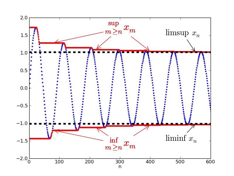
After
Front
ETH::2._Semester::Analysis::2._Folgen::3._Häufungspunkte::2._Limsup_und_Liminf
Die Grösse \[ \limsup_{n \rightarrow \infty} a_n = {{c1:: \lim_{n \rightarrow \infty} \sup \{a_k \mid k \ge n \} }}\] heisst Limes superior der Folge \(a_n\).
Back
ETH::2._Semester::Analysis::2._Folgen::3._Häufungspunkte::2._Limsup_und_Liminf
Die Grösse \[ \limsup_{n \rightarrow \infty} a_n = {{c1:: \lim_{n \rightarrow \infty} \sup \{a_k \mid k \ge n \} }}\] heisst Limes superior der Folge \(a_n\).
Das gleiche gilt für den Limes inferior.
Field-by-field Comparison
| Field |
Before |
After |
| Text |
Die Größe \[ \limsup_{n \rightarrow \infty} a_n = {{c1:: \lim_{n \rightarrow \infty} \sup \{a_k \mid k \ge n \} }}\] heisst <i>Limes superior</i> der Folge \(a_n\). |
Die Grösse \[ \limsup_{n \rightarrow \infty} a_n = {{c1:: \lim_{n \rightarrow \infty} \sup \{a_k \mid k \ge n \} }}\] heisst <i>Limes superior</i> der Folge \(a_n\). |
Tags:
ETH::2._Semester::Analysis::2._Folgen::3._Häufungspunkte::2._Limsup_und_Liminf
Note 98: ETH::2. Semester::Analysis
Deck: ETH::2. Semester::Analysis
Note Type: Horvath Classic
GUID: g;H{T:/_sJ
added
Previous
Note did not exist
New Note
Front
ETH::2._Semester::Analysis::5._Differentialrechnung::2._Differenzierbarkeit ETH::2._Semester::Analysis::Serie::8
Auf welchem Intervall ist die Funktion \(x \mapsto |x|\) differenzierbar?
- \((-1, 1)\)
- \((-1, 0)\)
Back
ETH::2._Semester::Analysis::5._Differentialrechnung::2._Differenzierbarkeit ETH::2._Semester::Analysis::Serie::8
Auf welchem Intervall ist die Funktion \(x \mapsto |x|\) differenzierbar?
- \((-1, 1)\)
- \((-1, 0)\)
(b) Auf \((-1, 0)\) stimmt \(|x|\) mit der differenzierbaren Funktion \(-x\) überein, ist dort also differenzierbar.
(a) ist falsch, da \(0 \in (-1, 1)\) und die Betragsfunktion in \(0\) nicht differenzierbar ist.
Field-by-field Comparison
| Field |
Before |
After |
| Front |
|
Auf welchem Intervall ist die Funktion \(x \mapsto |x|\) differenzierbar?<ol type="a"><li>\((-1, 1)\)</li><li>\((-1, 0)\)</li></ol> |
| Back |
|
<b>(b)</b> Auf \((-1, 0)\) stimmt \(|x|\) mit der differenzierbaren Funktion \(-x\) überein, ist dort also differenzierbar.<br><br>(a) ist falsch, da \(0 \in (-1, 1)\) und die Betragsfunktion in \(0\) nicht differenzierbar ist. |
Tags:
ETH::2._Semester::Analysis::5._Differentialrechnung::2._Differenzierbarkeit
ETH::2._Semester::Analysis::Serie::8
Note 99: ETH::2. Semester::Analysis
Deck: ETH::2. Semester::Analysis
Note Type: Horvath Cloze
GUID: g[Vr^Q|w!L
added
Previous
Note did not exist
New Note
Front
ETH::2._Semester::Analysis::6._Differentialgleichungen::4._Lineare_inhomogene::3._Ansatz_partikuläre_Lösung
Ansatz für die partikuläre Lösung bei einer Schwingung als Störfunktion
Störfunktion \(s(t) = A \sin(\omega t) + B \cos(\omega t)\):
\[ y(t) = C_1 \sin(\omega t) + C_2 \cos(\omega t) \]Spezialfall (Resonanz): Ist \(i\omega\) eine \(m\)-fache Nullstelle des charakteristischen Polynoms, so lautet der Ansatz
\[ y(t) = (C_1 \sin(\omega t) + C_2 \cos(\omega t))\, t^m \]
Back
ETH::2._Semester::Analysis::6._Differentialgleichungen::4._Lineare_inhomogene::3._Ansatz_partikuläre_Lösung
Ansatz für die partikuläre Lösung bei einer Schwingung als Störfunktion
Störfunktion \(s(t) = A \sin(\omega t) + B \cos(\omega t)\):
\[ y(t) = C_1 \sin(\omega t) + C_2 \cos(\omega t) \]Spezialfall (Resonanz): Ist \(i\omega\) eine \(m\)-fache Nullstelle des charakteristischen Polynoms, so lautet der Ansatz
\[ y(t) = (C_1 \sin(\omega t) + C_2 \cos(\omega t))\, t^m \]
Field-by-field Comparison
| Field |
Before |
After |
| Text |
|
<b>Ansatz für die partikuläre Lösung</b> bei einer <b>Schwingung</b> als Störfunktion<br>Störfunktion \(s(t) = A \sin(\omega t) + B \cos(\omega t)\):<br>\[ y(t) = {{c1::C_1 \sin(\omega t) + C_2 \cos(\omega t)}} \]<b>Spezialfall</b> (Resonanz): Ist \(i\omega\) eine \(m\)-fache Nullstelle des charakteristischen Polynoms, so lautet der Ansatz<br>\[ y(t) = {{c2::(C_1 \sin(\omega t) + C_2 \cos(\omega t))\, t^m}} \] |
Tags:
ETH::2._Semester::Analysis::6._Differentialgleichungen::4._Lineare_inhomogene::3._Ansatz_partikuläre_Lösung
Note 100: ETH::2. Semester::Analysis
Deck: ETH::2. Semester::Analysis
Note Type: Horvath Classic
GUID: h9gE!xi2:F
added
Previous
Note did not exist
New Note
Front
ETH::2._Semester::Analysis::5._Differentialrechnung::5._Extremalstellen ETH::2._Semester::Analysis::Serie::9
Welche der folgenden Schlüsse über eine differenzierbare Funktion \(f : (a, b) \rightarrow \mathbb{R}\) sind logisch korrekt?
- Die Funktion \(f\) hat in \(x_0 \in (a, b)\) ein Maximum, also ist \(f'(x_0) = 0\).
- Die Funktion \(f\) hat in \(x_0 \in (a, b)\) weder ein Maximum noch ein Minimum, also ist \(f'(x_0) \neq 0\).
- Die Funktion \(f\) ist links von \(x_0 \in (a, b)\) monoton fallend und rechts von \(x_0\) monoton wachsend, also ist \(x_0\) ein lokales Minimum.
- Die Funktion \(f\) ist monoton fallend, also ist \(f' \leq 0\).
- Die Funktion \(f\) ist monoton fallend, also ist \(f' < 0\).
- Die Funktion \(f\) ist streng monoton fallend, also ist \(f' < 0\).
Back
ETH::2._Semester::Analysis::5._Differentialrechnung::5._Extremalstellen ETH::2._Semester::Analysis::Serie::9
Welche der folgenden Schlüsse über eine differenzierbare Funktion \(f : (a, b) \rightarrow \mathbb{R}\) sind logisch korrekt?
- Die Funktion \(f\) hat in \(x_0 \in (a, b)\) ein Maximum, also ist \(f'(x_0) = 0\).
- Die Funktion \(f\) hat in \(x_0 \in (a, b)\) weder ein Maximum noch ein Minimum, also ist \(f'(x_0) \neq 0\).
- Die Funktion \(f\) ist links von \(x_0 \in (a, b)\) monoton fallend und rechts von \(x_0\) monoton wachsend, also ist \(x_0\) ein lokales Minimum.
- Die Funktion \(f\) ist monoton fallend, also ist \(f' \leq 0\).
- Die Funktion \(f\) ist monoton fallend, also ist \(f' < 0\).
- Die Funktion \(f\) ist streng monoton fallend, also ist \(f' < 0\).
(a), (c) und (d) sind korrekt.
(a) Innere Extremstelle einer differenzierbaren Funktion ist kritischer Punkt. (c) Fällt links und steigt rechts, liegt ein lokales Minimum vor. (d) Aus Monotonie folgt \(f' \leq 0\) als Grenzwert der Differenzenquotienten.
(b) ist falsch (Sattelpunkt, z.B. \(x^3\) bei \(0\)). (e) ist falsch (konstante Funktion: \(f' \equiv 0\)). (f) ist falsch (z.B. \(-x^3\) ist streng fallend mit \(f'(0) = 0\)).
Field-by-field Comparison
| Field |
Before |
After |
| Front |
|
Welche der folgenden Schlüsse über eine differenzierbare Funktion \(f : (a, b) \rightarrow \mathbb{R}\) sind logisch korrekt?<ol type="a"><li>Die Funktion \(f\) hat in \(x_0 \in (a, b)\) ein Maximum, also ist \(f'(x_0) = 0\).</li><li>Die Funktion \(f\) hat in \(x_0 \in (a, b)\) weder ein Maximum noch ein Minimum, also ist \(f'(x_0) \neq 0\).</li><li>Die Funktion \(f\) ist links von \(x_0 \in (a, b)\) monoton fallend und rechts von \(x_0\) monoton wachsend, also ist \(x_0\) ein lokales Minimum.</li><li>Die Funktion \(f\) ist monoton fallend, also ist \(f' \leq 0\).</li><li>Die Funktion \(f\) ist monoton fallend, also ist \(f' < 0\).</li><li>Die Funktion \(f\) ist streng monoton fallend, also ist \(f' < 0\).</li></ol> |
| Back |
|
<b>(a), (c) und (d)</b> sind korrekt.<br><br>(a) Innere Extremstelle einer differenzierbaren Funktion ist kritischer Punkt. (c) Fällt links und steigt rechts, liegt ein lokales Minimum vor. (d) Aus Monotonie folgt \(f' \leq 0\) als Grenzwert der Differenzenquotienten.<br><br>(b) ist falsch (Sattelpunkt, z.B. \(x^3\) bei \(0\)). (e) ist falsch (konstante Funktion: \(f' \equiv 0\)). (f) ist falsch (z.B. \(-x^3\) ist streng fallend mit \(f'(0) = 0\)). |
Tags:
ETH::2._Semester::Analysis::5._Differentialrechnung::5._Extremalstellen
ETH::2._Semester::Analysis::Serie::9
Note 101: ETH::2. Semester::Analysis
Deck: ETH::2. Semester::Analysis
Note Type: Horvath Cloze
GUID: is0]!/|g|u
modified
Before
Front
ETH::2._Semester::Analysis::1._Logik,_Mengen,_Zahlen::3._Zahlen::2._Infimum_Supremum
Beweis:
Für alle \(a < b\) in \(\mathbb{R}\) existiert ein \(\mathbb{Q}\) mit \(a < q < b\)
- {{c1:: Wähle nach Archimedischem Prinzip \(n \in \mathbb{N}\) so dass \(\frac{1}{n} < b - a\).}}
- {{c2:: \(\frac{m}{n} \mid m \in \mathbb{Z}\) diese Vielfache überdecken ganz \(\mathbb{R}\) in regelmäßigen Abständen von \(\frac{1}{n}\).}}
- {{c3::Wähle kleinstes \(m \in \mathbb{Z}\) mit \(\frac{m}{n} > a\) dann gilt \(\frac{m - 1}{n} \le a\) also \[ \frac{m}{n} = \frac{m - 1}{n} + \frac{1}{n} \le a + \frac{1}{n} < a + (b - a) = b \]}}
- {{c4:: Somit ist \(q = \frac{m}{n} \in \mathbb{Q}\) mit \(a < q < b\).}}
Back
ETH::2._Semester::Analysis::1._Logik,_Mengen,_Zahlen::3._Zahlen::2._Infimum_Supremum
Beweis:
Für alle \(a < b\) in \(\mathbb{R}\) existiert ein \(\mathbb{Q}\) mit \(a < q < b\)
- {{c1:: Wähle nach Archimedischem Prinzip \(n \in \mathbb{N}\) so dass \(\frac{1}{n} < b - a\).}}
- {{c2:: \(\frac{m}{n} \mid m \in \mathbb{Z}\) diese Vielfache überdecken ganz \(\mathbb{R}\) in regelmäßigen Abständen von \(\frac{1}{n}\).}}
- {{c3::Wähle kleinstes \(m \in \mathbb{Z}\) mit \(\frac{m}{n} > a\) dann gilt \(\frac{m - 1}{n} \le a\) also \[ \frac{m}{n} = \frac{m - 1}{n} + \frac{1}{n} \le a + \frac{1}{n} < a + (b - a) = b \]}}
- {{c4:: Somit ist \(q = \frac{m}{n} \in \mathbb{Q}\) mit \(a < q < b\).}}
After
Front
ETH::2._Semester::Analysis::1._Logik,_Mengen,_Zahlen::3._Zahlen::2._Infimum_Supremum
Beweis:
Für alle \(a < b\) in \(\mathbb{R}\) existiert ein \(\mathbb{Q}\) mit \(a < q < b\)
- {{c1:: Wähle nach Archimedischem Prinzip \(n \in \mathbb{N}\) so dass \(\frac{1}{n} < b - a\).}}
- {{c2:: \(\frac{m}{n} \mid m \in \mathbb{Z}\) diese Vielfache überdecken ganz \(\mathbb{R}\) in regelmässigen Abständen von \(\frac{1}{n}\).}}
- {{c3::Wähle kleinstes \(m \in \mathbb{Z}\) mit \(\frac{m}{n} > a\) dann gilt \(\frac{m - 1}{n} \le a\) also \[ \frac{m}{n} = \frac{m - 1}{n} + \frac{1}{n} \le a + \frac{1}{n} < a + (b - a) = b \]}}
- {{c4:: Somit ist \(q = \frac{m}{n} \in \mathbb{Q}\) mit \(a < q < b\).}}
Back
ETH::2._Semester::Analysis::1._Logik,_Mengen,_Zahlen::3._Zahlen::2._Infimum_Supremum
Beweis:
Für alle \(a < b\) in \(\mathbb{R}\) existiert ein \(\mathbb{Q}\) mit \(a < q < b\)
- {{c1:: Wähle nach Archimedischem Prinzip \(n \in \mathbb{N}\) so dass \(\frac{1}{n} < b - a\).}}
- {{c2:: \(\frac{m}{n} \mid m \in \mathbb{Z}\) diese Vielfache überdecken ganz \(\mathbb{R}\) in regelmässigen Abständen von \(\frac{1}{n}\).}}
- {{c3::Wähle kleinstes \(m \in \mathbb{Z}\) mit \(\frac{m}{n} > a\) dann gilt \(\frac{m - 1}{n} \le a\) also \[ \frac{m}{n} = \frac{m - 1}{n} + \frac{1}{n} \le a + \frac{1}{n} < a + (b - a) = b \]}}
- {{c4:: Somit ist \(q = \frac{m}{n} \in \mathbb{Q}\) mit \(a < q < b\).}}
Field-by-field Comparison
| Field |
Before |
After |
| Text |
Beweis: <br>Für alle \(a < b\) in \(\mathbb{R}\) existiert ein \(\mathbb{Q}\) mit \(a < q < b\)<br><ol><li>{{c1:: Wähle nach Archimedischem Prinzip \(n \in \mathbb{N}\) so dass \(\frac{1}{n} < b - a\).}}</li><li>{{c2:: \(\frac{m}{n} \mid m \in \mathbb{Z}\) diese Vielfache überdecken ganz \(\mathbb{R}\) in regelmäßigen Abständen von \(\frac{1}{n}\).}}</li><li>{{c3::Wähle kleinstes \(m \in \mathbb{Z}\) mit \(\frac{m}{n} > a\) dann gilt \(\frac{m - 1}{n} \le a\) also \[ \frac{m}{n} = \frac{m - 1}{n} + \frac{1}{n} \le a + \frac{1}{n} < a + (b - a) = b \]}}</li><li>{{c4:: Somit ist \(q = \frac{m}{n} \in \mathbb{Q}\) mit \(a < q < b\).}}</li></ol> |
Beweis: <br>Für alle \(a < b\) in \(\mathbb{R}\) existiert ein \(\mathbb{Q}\) mit \(a < q < b\)<br><ol><li>{{c1:: Wähle nach Archimedischem Prinzip \(n \in \mathbb{N}\) so dass \(\frac{1}{n} < b - a\).}}</li><li>{{c2:: \(\frac{m}{n} \mid m \in \mathbb{Z}\) diese Vielfache überdecken ganz \(\mathbb{R}\) in regelmässigen Abständen von \(\frac{1}{n}\).}}</li><li>{{c3::Wähle kleinstes \(m \in \mathbb{Z}\) mit \(\frac{m}{n} > a\) dann gilt \(\frac{m - 1}{n} \le a\) also \[ \frac{m}{n} = \frac{m - 1}{n} + \frac{1}{n} \le a + \frac{1}{n} < a + (b - a) = b \]}}</li><li>{{c4:: Somit ist \(q = \frac{m}{n} \in \mathbb{Q}\) mit \(a < q < b\).}}</li></ol> |
Tags:
ETH::2._Semester::Analysis::1._Logik,_Mengen,_Zahlen::3._Zahlen::2._Infimum_Supremum
Note 102: ETH::2. Semester::Analysis
Deck: ETH::2. Semester::Analysis
Note Type: Horvath Cloze
GUID: ki6gGw!;6e
added
Previous
Note did not exist
New Note
Front
ETH::2._Semester::Analysis::6._Differentialgleichungen::4._Lineare_inhomogene::1._Lösungsstruktur
Lösungsstruktur linearer, inhomogener DGl
Ist \(y_p(x)\) eine partikuläre Lösung der inhomogenen DGl und \(y_h(x)\) die allgemeine Lösung der dazugehörigen homogenen DGl, so ist die allgemeine Lösung der inhomogenen DGl
\[ y(x) = y_h(x) + y_p(x) \]
Back
ETH::2._Semester::Analysis::6._Differentialgleichungen::4._Lineare_inhomogene::1._Lösungsstruktur
Lösungsstruktur linearer, inhomogener DGl
Ist \(y_p(x)\) eine partikuläre Lösung der inhomogenen DGl und \(y_h(x)\) die allgemeine Lösung der dazugehörigen homogenen DGl, so ist die allgemeine Lösung der inhomogenen DGl
\[ y(x) = y_h(x) + y_p(x) \]
Field-by-field Comparison
| Field |
Before |
After |
| Text |
|
<b>Lösungsstruktur linearer, inhomogener DGl</b><br>Ist \(y_p(x)\) {{c1::eine partikuläre Lösung der inhomogenen DGl}} und \(y_h(x)\) {{c2::die allgemeine Lösung der dazugehörigen homogenen DGl}}, so ist die allgemeine Lösung der inhomogenen DGl<br>\[ y(x) = {{c3::y_h(x) + y_p(x)}} \] |
Tags:
ETH::2._Semester::Analysis::6._Differentialgleichungen::4._Lineare_inhomogene::1._Lösungsstruktur
Note 103: ETH::2. Semester::Analysis
Deck: ETH::2. Semester::Analysis
Note Type: Horvath Classic
GUID: l%kph3(F:=
added
Previous
Note did not exist
New Note
Front
ETH::2._Semester::Analysis::5._Differentialrechnung::4._Ableitungsregeln::2._Rechenregeln ETH::2._Semester::Analysis::Serie::8
Was ist die Ableitung von \(\ln(x^2 - 1)\)?
- \(\frac{2x}{x^2 - 1}\)
- \(\frac{1}{x^2 - 1}\)
- \(\frac{1}{2x}\)
- \(\frac{x^2 - 1}{2x}\)
Back
ETH::2._Semester::Analysis::5._Differentialrechnung::4._Ableitungsregeln::2._Rechenregeln ETH::2._Semester::Analysis::Serie::8
Was ist die Ableitung von \(\ln(x^2 - 1)\)?
- \(\frac{2x}{x^2 - 1}\)
- \(\frac{1}{x^2 - 1}\)
- \(\frac{1}{2x}\)
- \(\frac{x^2 - 1}{2x}\)
(a) Mit \(g(y) = \ln(y)\), \(h(x) = x^2 - 1\) ist \(g'(y) = \tfrac{1}{y}\), \(h'(x) = 2x\), also nach Kettenregel \(f'(x) = \tfrac{1}{h(x)} h'(x) = \tfrac{2x}{x^2 - 1}\).
(b) vergisst die innere Ableitung. (c) und (d) verwenden die Kettenregel falsch.
Field-by-field Comparison
| Field |
Before |
After |
| Front |
|
Was ist die Ableitung von \(\ln(x^2 - 1)\)?<ol type="a"><li>\(\frac{2x}{x^2 - 1}\)</li><li>\(\frac{1}{x^2 - 1}\)</li><li>\(\frac{1}{2x}\)</li><li>\(\frac{x^2 - 1}{2x}\)</li></ol> |
| Back |
|
<b>(a)</b> Mit \(g(y) = \ln(y)\), \(h(x) = x^2 - 1\) ist \(g'(y) = \tfrac{1}{y}\), \(h'(x) = 2x\), also nach Kettenregel \(f'(x) = \tfrac{1}{h(x)} h'(x) = \tfrac{2x}{x^2 - 1}\).<br><br>(b) vergisst die innere Ableitung. (c) und (d) verwenden die Kettenregel falsch. |
Tags:
ETH::2._Semester::Analysis::5._Differentialrechnung::4._Ableitungsregeln::2._Rechenregeln
ETH::2._Semester::Analysis::Serie::8
Note 104: ETH::2. Semester::Analysis
Deck: ETH::2. Semester::Analysis
Note Type: Horvath Classic
GUID: li|o~y<|Xv
added
Previous
Note did not exist
New Note
Front
ETH::2._Semester::Analysis::5._Differentialrechnung::4._Ableitungsregeln::2._Rechenregeln ETH::2._Semester::Analysis::Serie::8
Leiten Sie die Funktion \(\frac{1}{\cos(x)} e^{\sin(x)}\) ab.
- \(e^{\sin(x)}\)
- \(\tan(x) e^{\sin(x)}\)
- \(e^{\sin(x)}\left(1 + \frac{\sin(x)}{\cos^2(x)}\right)\)
- \(\left(1 - \frac{\sin(x)}{\cos^2(x)}\right) e^{\cos(x)}\)
Back
ETH::2._Semester::Analysis::5._Differentialrechnung::4._Ableitungsregeln::2._Rechenregeln ETH::2._Semester::Analysis::Serie::8
Leiten Sie die Funktion \(\frac{1}{\cos(x)} e^{\sin(x)}\) ab.
- \(e^{\sin(x)}\)
- \(\tan(x) e^{\sin(x)}\)
- \(e^{\sin(x)}\left(1 + \frac{\sin(x)}{\cos^2(x)}\right)\)
- \(\left(1 - \frac{\sin(x)}{\cos^2(x)}\right) e^{\cos(x)}\)
(c) Mit Produkt- und Kettenregel: \(\tfrac{d}{dx}\big(\tfrac{1}{\cos(x)}\big) e^{\sin(x)} + \tfrac{1}{\cos(x)} \cos(x) e^{\sin(x)} = \tfrac{\sin(x)}{\cos^2(x)} e^{\sin(x)} + e^{\sin(x)} = \big(1 + \tfrac{\sin(x)}{\cos^2(x)}\big) e^{\sin(x)}\).
(a) vergisst die Ableitung von \(\tfrac{1}{\cos(x)}\). (b) leitet falsch ab. (d) setzt die Ableitung in den Exponenten und hat ein falsches Vorzeichen.
Field-by-field Comparison
| Field |
Before |
After |
| Front |
|
Leiten Sie die Funktion \(\frac{1}{\cos(x)} e^{\sin(x)}\) ab.<ol type="a"><li>\(e^{\sin(x)}\)</li><li>\(\tan(x) e^{\sin(x)}\)</li><li>\(e^{\sin(x)}\left(1 + \frac{\sin(x)}{\cos^2(x)}\right)\)</li><li>\(\left(1 - \frac{\sin(x)}{\cos^2(x)}\right) e^{\cos(x)}\)</li></ol> |
| Back |
|
<b>(c)</b> Mit Produkt- und Kettenregel: \(\tfrac{d}{dx}\big(\tfrac{1}{\cos(x)}\big) e^{\sin(x)} + \tfrac{1}{\cos(x)} \cos(x) e^{\sin(x)} = \tfrac{\sin(x)}{\cos^2(x)} e^{\sin(x)} + e^{\sin(x)} = \big(1 + \tfrac{\sin(x)}{\cos^2(x)}\big) e^{\sin(x)}\).<br><br>(a) vergisst die Ableitung von \(\tfrac{1}{\cos(x)}\). (b) leitet falsch ab. (d) setzt die Ableitung in den Exponenten und hat ein falsches Vorzeichen. |
Tags:
ETH::2._Semester::Analysis::5._Differentialrechnung::4._Ableitungsregeln::2._Rechenregeln
ETH::2._Semester::Analysis::Serie::8
Note 105: ETH::2. Semester::Analysis
Deck: ETH::2. Semester::Analysis
Note Type: Horvath Cloze
GUID: oY{~s0cb5-
modified
Before
Front
ETH::2._Semester::Analysis::1._Logik,_Mengen,_Zahlen::3._Zahlen::4._Komplexe_Zahlen::5._Komplexe_Polynome
Die nicht-reellen Nullstellen eines Polynoms mit reellen Koeffizienten treten in komplex konjugierten Paaren auf.
Back
ETH::2._Semester::Analysis::1._Logik,_Mengen,_Zahlen::3._Zahlen::4._Komplexe_Zahlen::5._Komplexe_Polynome
Die nicht-reellen Nullstellen eines Polynoms mit reellen Koeffizienten treten in komplex konjugierten Paaren auf.
Beispiel: Heißt, wenn \(3 + i4\) eine Wurzel ist, ist es auch \(3 - i4\)!
After
Front
ETH::2._Semester::Analysis::1._Logik,_Mengen,_Zahlen::3._Zahlen::4._Komplexe_Zahlen::5._Komplexe_Polynome
Die nicht-reellen Nullstellen eines Polynoms mit reellen Koeffizienten treten in komplex konjugierten Paaren auf.
Back
ETH::2._Semester::Analysis::1._Logik,_Mengen,_Zahlen::3._Zahlen::4._Komplexe_Zahlen::5._Komplexe_Polynome
Die nicht-reellen Nullstellen eines Polynoms mit reellen Koeffizienten treten in komplex konjugierten Paaren auf.
Beispiel: Heisst, wenn \(3 + i4\) eine Wurzel ist, ist es auch \(3 - i4\)!
Field-by-field Comparison
| Field |
Before |
After |
| Extra |
<div><b>Beispiel</b>: Heißt, wenn \(3 + i4\) eine Wurzel ist, ist es auch \(3 - i4\)!</div> |
<div><b>Beispiel</b>: Heisst, wenn \(3 + i4\) eine Wurzel ist, ist es auch \(3 - i4\)!</div> |
Tags:
ETH::2._Semester::Analysis::1._Logik,_Mengen,_Zahlen::3._Zahlen::4._Komplexe_Zahlen::5._Komplexe_Polynome
Note 106: ETH::2. Semester::Analysis
Deck: ETH::2. Semester::Analysis
Note Type: Horvath Cloze
GUID: qn/,_xx>>5
modified
Before
Front
ETH::2._Semester::Analysis::1._Logik,_Mengen,_Zahlen::3._Zahlen::2._Infimum_Supremum
Infimum oder Supremum können \(\pm \infty\) sein, Maximum oder Minimum jedoch nicht!
Back
ETH::2._Semester::Analysis::1._Logik,_Mengen,_Zahlen::3._Zahlen::2._Infimum_Supremum
Infimum oder Supremum können \(\pm \infty\) sein, Maximum oder Minimum jedoch nicht!
\(\infty\) ist keine reelle Zahl (für jede reelle Zahl, gibt es eine größere), kann also nicht in einer Menge enthalten sein.
After
Front
ETH::2._Semester::Analysis::1._Logik,_Mengen,_Zahlen::3._Zahlen::2._Infimum_Supremum
Infimum oder Supremum können \(\pm \infty\) sein, Maximum oder Minimum jedoch nicht!
Back
ETH::2._Semester::Analysis::1._Logik,_Mengen,_Zahlen::3._Zahlen::2._Infimum_Supremum
Infimum oder Supremum können \(\pm \infty\) sein, Maximum oder Minimum jedoch nicht!
\(\infty\) ist keine reelle Zahl (für jede reelle Zahl, gibt es eine grössere), kann also nicht in einer Menge enthalten sein.
Field-by-field Comparison
| Field |
Before |
After |
| Extra |
\(\infty\) ist keine reelle Zahl (für jede reelle Zahl, gibt es eine größere), kann also nicht in einer Menge enthalten sein. |
\(\infty\) ist keine reelle Zahl (für jede reelle Zahl, gibt es eine grössere), kann also nicht in einer Menge enthalten sein. |
Tags:
ETH::2._Semester::Analysis::1._Logik,_Mengen,_Zahlen::3._Zahlen::2._Infimum_Supremum
Note 107: ETH::2. Semester::Analysis
Deck: ETH::2. Semester::Analysis
Note Type: Horvath Classic
GUID: s%%xrPO*G#
added
Previous
Note did not exist
New Note
Front
ETH::2._Semester::Analysis::5._Differentialrechnung::4._Ableitungsregeln::2._Rechenregeln ETH::2._Semester::Analysis::Serie::8
Bestimmen Sie die Ableitung der Funktion \(e^{\frac{x^3 - x}{1 + \cos^2(x)}}\).
- \(e^{\frac{x^3 - x}{1 + \cos^2(x)}}\)
- \(\frac{(3x^2 - 1)(1 + \cos^2(x)) + 2(x^3 - x)\cos(x)\sin(x)}{(1 + \cos^2(x))^2}\, e^{\frac{x^3 - x}{1 + \cos^2(x)}}\)
- \(e^{\frac{(3x^2 - 1)(1 + \cos^2(x)) + 2(x^3 - x)\cos(x)\sin(x)}{(1 + \cos^2(x))^2}}\)
- \(\frac{3x^2 - 1}{-2\cos(x)\sin(x)}\, e^{\frac{x^3 - x}{1 + \cos^2(x)}}\)
Back
ETH::2._Semester::Analysis::5._Differentialrechnung::4._Ableitungsregeln::2._Rechenregeln ETH::2._Semester::Analysis::Serie::8
Bestimmen Sie die Ableitung der Funktion \(e^{\frac{x^3 - x}{1 + \cos^2(x)}}\).
- \(e^{\frac{x^3 - x}{1 + \cos^2(x)}}\)
- \(\frac{(3x^2 - 1)(1 + \cos^2(x)) + 2(x^3 - x)\cos(x)\sin(x)}{(1 + \cos^2(x))^2}\, e^{\frac{x^3 - x}{1 + \cos^2(x)}}\)
- \(e^{\frac{(3x^2 - 1)(1 + \cos^2(x)) + 2(x^3 - x)\cos(x)\sin(x)}{(1 + \cos^2(x))^2}}\)
- \(\frac{3x^2 - 1}{-2\cos(x)\sin(x)}\, e^{\frac{x^3 - x}{1 + \cos^2(x)}}\)
(b) Mit \(g(y) = e^y\) und \(h(x) = \tfrac{x^3 - x}{1 + \cos^2(x)}\) liefert die Kettenregel \(f'(x) = e^{h(x)} h'(x)\). Der Vorfaktor \(h'(x)\) ergibt sich mit der Quotientenregel zum Zähler oben.
(a) vergisst die innere Ableitung. (c) setzt die Ableitung fälschlich in den Exponenten. (d) wendet die Quotientenregel falsch an.
Field-by-field Comparison
| Field |
Before |
After |
| Front |
|
Bestimmen Sie die Ableitung der Funktion \(e^{\frac{x^3 - x}{1 + \cos^2(x)}}\).<ol type="a"><li>\(e^{\frac{x^3 - x}{1 + \cos^2(x)}}\)</li><li>\(\frac{(3x^2 - 1)(1 + \cos^2(x)) + 2(x^3 - x)\cos(x)\sin(x)}{(1 + \cos^2(x))^2}\, e^{\frac{x^3 - x}{1 + \cos^2(x)}}\)</li><li>\(e^{\frac{(3x^2 - 1)(1 + \cos^2(x)) + 2(x^3 - x)\cos(x)\sin(x)}{(1 + \cos^2(x))^2}}\)</li><li>\(\frac{3x^2 - 1}{-2\cos(x)\sin(x)}\, e^{\frac{x^3 - x}{1 + \cos^2(x)}}\)</li></ol> |
| Back |
|
<b>(b)</b> Mit \(g(y) = e^y\) und \(h(x) = \tfrac{x^3 - x}{1 + \cos^2(x)}\) liefert die Kettenregel \(f'(x) = e^{h(x)} h'(x)\). Der Vorfaktor \(h'(x)\) ergibt sich mit der Quotientenregel zum Zähler oben.<br><br>(a) vergisst die innere Ableitung. (c) setzt die Ableitung fälschlich in den Exponenten. (d) wendet die Quotientenregel falsch an. |
Tags:
ETH::2._Semester::Analysis::5._Differentialrechnung::4._Ableitungsregeln::2._Rechenregeln
ETH::2._Semester::Analysis::Serie::8
Note 108: ETH::2. Semester::Analysis
Deck: ETH::2. Semester::Analysis
Note Type: Horvath Classic
GUID: sP=)zCvc`~
added
Previous
Note did not exist
New Note
Front
ETH::2._Semester::Analysis::4._Funktionen::3._Grenzwerte ETH::2._Semester::Analysis::Serie::7
Welche der folgenden Bedingungen impliziert
nicht, dass \(f : \mathbb{R} \rightarrow \mathbb{R}\) stetig ist?
- Es gibt \(C \geq 0\), so dass \(|f(x) - f(y)| \leq C|x - y|\) für alle \(x, y \in \mathbb{R}\).
- Es gibt \(C \geq 0\), so dass \(|f(x) - f(y)| \leq C|x - y|\) für alle \(x, y \in \mathbb{R}\) mit \(|x - y| \geq 1\).
- Es gibt \(C \geq 0\), so dass \(|f(x) - f(y)| \leq C|x - y|^2\) für alle \(x, y \in \mathbb{R}\) mit \(|x - y| \leq 1\).
Back
ETH::2._Semester::Analysis::4._Funktionen::3._Grenzwerte ETH::2._Semester::Analysis::Serie::7
Welche der folgenden Bedingungen impliziert
nicht, dass \(f : \mathbb{R} \rightarrow \mathbb{R}\) stetig ist?
- Es gibt \(C \geq 0\), so dass \(|f(x) - f(y)| \leq C|x - y|\) für alle \(x, y \in \mathbb{R}\).
- Es gibt \(C \geq 0\), so dass \(|f(x) - f(y)| \leq C|x - y|\) für alle \(x, y \in \mathbb{R}\) mit \(|x - y| \geq 1\).
- Es gibt \(C \geq 0\), so dass \(|f(x) - f(y)| \leq C|x - y|^2\) für alle \(x, y \in \mathbb{R}\) mit \(|x - y| \leq 1\).
(b) Diese Bedingung impliziert keine Stetigkeit. Gegenbeispiel: \(C = 1\), \(f(x) = 0\) für \(x < 0\) und \(f(x) = 1\) für \(x \geq 0\). Diese Funktion ist in \(0\) unstetig, erfüllt aber \(|f(x) - f(y)| \leq 1 \leq |x - y|\) für alle \(x, y\) mit \(|x - y| \geq 1\).
(a) ist eine Lipschitz-Bedingung und impliziert Stetigkeit (\(\delta = \varepsilon / C\)). (c) impliziert ebenfalls Stetigkeit (\(\delta = \min\{\varepsilon/C, 1\}\)).
Field-by-field Comparison
| Field |
Before |
After |
| Front |
|
Welche der folgenden Bedingungen impliziert <b>nicht</b>, dass \(f : \mathbb{R} \rightarrow \mathbb{R}\) stetig ist?<ol type="a"><li>Es gibt \(C \geq 0\), so dass \(|f(x) - f(y)| \leq C|x - y|\) für alle \(x, y \in \mathbb{R}\).</li><li>Es gibt \(C \geq 0\), so dass \(|f(x) - f(y)| \leq C|x - y|\) für alle \(x, y \in \mathbb{R}\) mit \(|x - y| \geq 1\).</li><li>Es gibt \(C \geq 0\), so dass \(|f(x) - f(y)| \leq C|x - y|^2\) für alle \(x, y \in \mathbb{R}\) mit \(|x - y| \leq 1\).</li></ol> |
| Back |
|
<b>(b)</b> Diese Bedingung impliziert keine Stetigkeit. Gegenbeispiel: \(C = 1\), \(f(x) = 0\) für \(x < 0\) und \(f(x) = 1\) für \(x \geq 0\). Diese Funktion ist in \(0\) unstetig, erfüllt aber \(|f(x) - f(y)| \leq 1 \leq |x - y|\) für alle \(x, y\) mit \(|x - y| \geq 1\).<br><br>(a) ist eine Lipschitz-Bedingung und impliziert Stetigkeit (\(\delta = \varepsilon / C\)). (c) impliziert ebenfalls Stetigkeit (\(\delta = \min\{\varepsilon/C, 1\}\)). |
Tags:
ETH::2._Semester::Analysis::4._Funktionen::3._Grenzwerte
ETH::2._Semester::Analysis::Serie::7
Note 109: ETH::2. Semester::Analysis
Deck: ETH::2. Semester::Analysis
Note Type: Horvath Cloze
GUID: s{-]C1^cF3
modified
Before
Front
ETH::2._Semester::Analysis::1._Logik,_Mengen,_Zahlen::3._Zahlen
Das Minimum/Maximum kann nicht \(\infty\) oder \(-\infty\) sein, weil es laut Archimedischem Prinzip immer größere/kleinere natürliche Zahlen gibt.
Back
ETH::2._Semester::Analysis::1._Logik,_Mengen,_Zahlen::3._Zahlen
Das Minimum/Maximum kann nicht \(\infty\) oder \(-\infty\) sein, weil es laut Archimedischem Prinzip immer größere/kleinere natürliche Zahlen gibt.
After
Front
ETH::2._Semester::Analysis::1._Logik,_Mengen,_Zahlen::3._Zahlen
Das Minimum/Maximum kann nicht \(\infty\) oder \(-\infty\) sein, weil es laut Archimedischem Prinzip immer grössere/kleinere natürliche Zahlen gibt.
Back
ETH::2._Semester::Analysis::1._Logik,_Mengen,_Zahlen::3._Zahlen
Das Minimum/Maximum kann nicht \(\infty\) oder \(-\infty\) sein, weil es laut Archimedischem Prinzip immer grössere/kleinere natürliche Zahlen gibt.
Field-by-field Comparison
| Field |
Before |
After |
| Text |
<div>Das Minimum/Maximum <b>kann nicht</b> {{c1:: \(\infty\) oder \(-\infty\)}} sein, weil {{c1::es laut Archimedischem Prinzip immer größere/kleinere natürliche Zahlen gibt}}.</div> |
<div>Das Minimum/Maximum <b>kann nicht</b> {{c1:: \(\infty\) oder \(-\infty\)}} sein, weil {{c1::es laut Archimedischem Prinzip immer grössere/kleinere natürliche Zahlen gibt}}.</div> |
Tags:
ETH::2._Semester::Analysis::1._Logik,_Mengen,_Zahlen::3._Zahlen
Note 110: ETH::2. Semester::Analysis
Deck: ETH::2. Semester::Analysis
Note Type: Horvath Cloze
GUID: t70~XZk{wJ
modified
Before
Front
ETH::2._Semester::Analysis::4._Funktionen::1._Grundlagen
Eine Funktion \(f: D \rightarrow R\) hat {{c1::einen Definitionsbereich \(\text{domain}(f) = \mathbb{D}(f) = D\)}} und {{c2::einen Wertebereich \(\text{range/image}(f) = R\)}}.
Back
ETH::2._Semester::Analysis::4._Funktionen::1._Grundlagen
Eine Funktion \(f: D \rightarrow R\) hat {{c1::einen Definitionsbereich \(\text{domain}(f) = \mathbb{D}(f) = D\)}} und {{c2::einen Wertebereich \(\text{range/image}(f) = R\)}}.
Der Input heißt unabhängige Variable (Argument) und der Output abhängige Variable.
After
Front
ETH::2._Semester::Analysis::4._Funktionen::1._Grundlagen
Eine Funktion \(f: D \rightarrow R\) hat {{c1::einen Definitionsbereich \(\text{domain}(f) = \mathbb{D}(f) = D\)}} und {{c2::einen Wertebereich \(\text{range/image}(f) = R\)}}.
Back
ETH::2._Semester::Analysis::4._Funktionen::1._Grundlagen
Eine Funktion \(f: D \rightarrow R\) hat {{c1::einen Definitionsbereich \(\text{domain}(f) = \mathbb{D}(f) = D\)}} und {{c2::einen Wertebereich \(\text{range/image}(f) = R\)}}.
Der Input heisst unabhängige Variable (Argument) und der Output abhängige Variable.
Field-by-field Comparison
| Field |
Before |
After |
| Extra |
<div>Der Input heißt unabhängige Variable (Argument) und der Output abhängige Variable.</div> |
<div>Der Input heisst unabhängige Variable (Argument) und der Output abhängige Variable.</div> |
Tags:
ETH::2._Semester::Analysis::4._Funktionen::1._Grundlagen
Note 111: ETH::2. Semester::Analysis
Deck: ETH::2. Semester::Analysis
Note Type: Horvath Classic
GUID: u*d5<@LyK@
modified
Before
Front
ETH::2._Semester::Analysis::2._Folgen::2._Konvergenz::5._Tricks
Trick: Fixpunkt
Sei eine Folge rekursiv definiert durch \(a_1 = c\) und \(a_{n+1} = f(a_n)\).
Back
ETH::2._Semester::Analysis::2._Folgen::2._Konvergenz::5._Tricks
Trick: Fixpunkt
Sei eine Folge rekursiv definiert durch \(a_1 = c\) und \(a_{n+1} = f(a_n)\).
Falls \((a_n)\) konvergiert (z.B. nach Weierstrass), setzt man \(l = \lim_{n \to \infty} a_n \) \(= \lim_{n \to \infty} a_{n+1}\) und erhält die Fixpunktgleichung: \(l = f(l)\)
Man löst diese Gleichung nach \(l\) auf und schließt anhand der Eigenschaften der Folge (Vorzeichen, Monotonie, Beschränktheit) aus, welcher Kandidat der tatsächliche Grenzwert ist.
After
Front
ETH::2._Semester::Analysis::2._Folgen::2._Konvergenz::5._Tricks
Trick: Fixpunkt
Sei eine Folge rekursiv definiert durch \(a_1 = c\) und \(a_{n+1} = f(a_n)\).
Back
ETH::2._Semester::Analysis::2._Folgen::2._Konvergenz::5._Tricks
Trick: Fixpunkt
Sei eine Folge rekursiv definiert durch \(a_1 = c\) und \(a_{n+1} = f(a_n)\).
Falls \((a_n)\) konvergiert (z.B. nach Weierstrass), setzt man \(l = \lim_{n \to \infty} a_n \) \(= \lim_{n \to \infty} a_{n+1}\) und erhält die Fixpunktgleichung: \(l = f(l)\)
Man löst diese Gleichung nach \(l\) auf und schliesst anhand der Eigenschaften der Folge (Vorzeichen, Monotonie, Beschränktheit) aus, welcher Kandidat der tatsächliche Grenzwert ist.
Field-by-field Comparison
| Field |
Before |
After |
| Back |
Falls \((a_n)\) konvergiert (z.B. nach Weierstrass), setzt man \(l = \lim_{n \to \infty} a_n \) \(= \lim_{n \to \infty} a_{n+1}\) und erhält die Fixpunktgleichung: \(l = f(l)\) <br><br>Man löst diese Gleichung nach \(l\) auf und schließt anhand der Eigenschaften der Folge (Vorzeichen, Monotonie, Beschränktheit) aus, welcher Kandidat der tatsächliche Grenzwert ist. |
Falls \((a_n)\) konvergiert (z.B. nach Weierstrass), setzt man \(l = \lim_{n \to \infty} a_n \) \(= \lim_{n \to \infty} a_{n+1}\) und erhält die Fixpunktgleichung: \(l = f(l)\) <br><br>Man löst diese Gleichung nach \(l\) auf und schliesst anhand der Eigenschaften der Folge (Vorzeichen, Monotonie, Beschränktheit) aus, welcher Kandidat der tatsächliche Grenzwert ist. |
Tags:
ETH::2._Semester::Analysis::2._Folgen::2._Konvergenz::5._Tricks
Note 112: ETH::2. Semester::Analysis
Deck: ETH::2. Semester::Analysis
Note Type: Horvath Classic
GUID: vDO}ywdMfl
added
Previous
Note did not exist
New Note
Front
ETH::2._Semester::Analysis::4._Funktionen::3._Grenzwerte ETH::2._Semester::Analysis::Serie::10
Seien \(f, g : \mathbb{R} \rightarrow \mathbb{R}\) mit \(g(x) \neq 0\) für alle \(x\). Wir nehmen an, dass \(\lim_{x \to \infty} f(x) = \infty\) und \(\lim_{x \to \infty} g(x) = -\infty\). Welche der folgenden Aussagen sind korrekt?
- Es ist möglich, dass \(\lim_{x \to \infty} \frac{f(x)}{g(x)} = -2\).
- Es ist möglich, dass \(\lim_{x \to \infty} \frac{f(x)}{g(x)} = \infty\).
- Es ist möglich, dass \(\lim_{x \to \infty} \frac{f(x)}{g(x)} = -\infty\).
Back
ETH::2._Semester::Analysis::4._Funktionen::3._Grenzwerte ETH::2._Semester::Analysis::Serie::10
Seien \(f, g : \mathbb{R} \rightarrow \mathbb{R}\) mit \(g(x) \neq 0\) für alle \(x\). Wir nehmen an, dass \(\lim_{x \to \infty} f(x) = \infty\) und \(\lim_{x \to \infty} g(x) = -\infty\). Welche der folgenden Aussagen sind korrekt?
- Es ist möglich, dass \(\lim_{x \to \infty} \frac{f(x)}{g(x)} = -2\).
- Es ist möglich, dass \(\lim_{x \to \infty} \frac{f(x)}{g(x)} = \infty\).
- Es ist möglich, dass \(\lim_{x \to \infty} \frac{f(x)}{g(x)} = -\infty\).
(a) und (c) sind korrekt.
(a) Beispiel \(f(x) = 2x\), \(g(x) = -x\): \(\tfrac{f}{g} \to -2\). (c) Beispiel \(f(x) = x^2\), \(g(x) = -x\): \(\tfrac{f}{g} \to -\infty\).
(b) ist falsch: für grosse \(x\) ist \(f(x) > 0\) und \(g(x) < 0\), also \(\tfrac{f}{g} < 0\), und der Grenzwert kann nicht \(+\infty\) sein.
Field-by-field Comparison
| Field |
Before |
After |
| Front |
|
Seien \(f, g : \mathbb{R} \rightarrow \mathbb{R}\) mit \(g(x) \neq 0\) für alle \(x\). Wir nehmen an, dass \(\lim_{x \to \infty} f(x) = \infty\) und \(\lim_{x \to \infty} g(x) = -\infty\). Welche der folgenden Aussagen sind korrekt?<ol type="a"><li>Es ist möglich, dass \(\lim_{x \to \infty} \frac{f(x)}{g(x)} = -2\).</li><li>Es ist möglich, dass \(\lim_{x \to \infty} \frac{f(x)}{g(x)} = \infty\).</li><li>Es ist möglich, dass \(\lim_{x \to \infty} \frac{f(x)}{g(x)} = -\infty\).</li></ol> |
| Back |
|
<b>(a) und (c)</b> sind korrekt.<br><br>(a) Beispiel \(f(x) = 2x\), \(g(x) = -x\): \(\tfrac{f}{g} \to -2\). (c) Beispiel \(f(x) = x^2\), \(g(x) = -x\): \(\tfrac{f}{g} \to -\infty\).<br><br>(b) ist falsch: für grosse \(x\) ist \(f(x) > 0\) und \(g(x) < 0\), also \(\tfrac{f}{g} < 0\), und der Grenzwert kann nicht \(+\infty\) sein. |
Tags:
ETH::2._Semester::Analysis::4._Funktionen::3._Grenzwerte
ETH::2._Semester::Analysis::Serie::10
Note 113: ETH::2. Semester::Analysis
Deck: ETH::2. Semester::Analysis
Note Type: Horvath Classic
GUID: xWRxdGcaz.
added
Previous
Note did not exist
New Note
Front
ETH::2._Semester::Analysis::5._Differentialrechnung::9._Taylor::1._Taylorpolynom ETH::2._Semester::Analysis::Serie::10
Welches der untenstehenden Polynome ist das Taylorpolynom 2. Ordnung der Funktion \(f(x) = x^{1/3}\) an der Stelle \(x_0 = 8\)?
- \(P_2(x) = 2 + \frac{1}{12} x - \frac{1}{288} x^2\)
- \(P_2(x) = 2 + \frac{1}{12}(x - 8) - \frac{1}{144}(x - 8)^2\)
- \(P_2(x) = 2 + \frac{1}{12}(x - 8) - \frac{1}{288}(x - 8)^2\)
Back
ETH::2._Semester::Analysis::5._Differentialrechnung::9._Taylor::1._Taylorpolynom ETH::2._Semester::Analysis::Serie::10
Welches der untenstehenden Polynome ist das Taylorpolynom 2. Ordnung der Funktion \(f(x) = x^{1/3}\) an der Stelle \(x_0 = 8\)?
- \(P_2(x) = 2 + \frac{1}{12} x - \frac{1}{288} x^2\)
- \(P_2(x) = 2 + \frac{1}{12}(x - 8) - \frac{1}{144}(x - 8)^2\)
- \(P_2(x) = 2 + \frac{1}{12}(x - 8) - \frac{1}{288}(x - 8)^2\)
(c) Mit \(f(8) = 2\), \(f'(8) = \tfrac{1}{12}\), \(f''(8) = -\tfrac{1}{144}\) ist der quadratische Koeffizient \(\tfrac{1}{2!} f''(8) = -\tfrac{1}{288}\), und die Potenzen sind in \((x - 8)\).
(a) verwendet Potenzen von \(x\) statt \((x - 8)\). (b) vergisst die Division durch \(2!\).
Field-by-field Comparison
| Field |
Before |
After |
| Front |
|
Welches der untenstehenden Polynome ist das Taylorpolynom 2. Ordnung der Funktion \(f(x) = x^{1/3}\) an der Stelle \(x_0 = 8\)?<ol type="a"><li>\(P_2(x) = 2 + \frac{1}{12} x - \frac{1}{288} x^2\)</li><li>\(P_2(x) = 2 + \frac{1}{12}(x - 8) - \frac{1}{144}(x - 8)^2\)</li><li>\(P_2(x) = 2 + \frac{1}{12}(x - 8) - \frac{1}{288}(x - 8)^2\)</li></ol> |
| Back |
|
<b>(c)</b> Mit \(f(8) = 2\), \(f'(8) = \tfrac{1}{12}\), \(f''(8) = -\tfrac{1}{144}\) ist der quadratische Koeffizient \(\tfrac{1}{2!} f''(8) = -\tfrac{1}{288}\), und die Potenzen sind in \((x - 8)\).<br><br>(a) verwendet Potenzen von \(x\) statt \((x - 8)\). (b) vergisst die Division durch \(2!\). |
Tags:
ETH::2._Semester::Analysis::5._Differentialrechnung::9._Taylor::1._Taylorpolynom
ETH::2._Semester::Analysis::Serie::10
Note 114: ETH::2. Semester::Analysis
Deck: ETH::2. Semester::Analysis
Note Type: Horvath Cloze
GUID: x_+o+alk&1
modified
Before
Front
ETH::2._Semester::Analysis::4._Funktionen::2._Properties
Der Graph einer Funktion heißt linksgekrümmt (Konvex) falls der Graph eine Linkskurve vollführt / der Graph unterhalb der Sekante ist.
Back
ETH::2._Semester::Analysis::4._Funktionen::2._Properties
Der Graph einer Funktion heißt linksgekrümmt (Konvex) falls der Graph eine Linkskurve vollführt / der Graph unterhalb der Sekante ist.
After
Front
ETH::2._Semester::Analysis::4._Funktionen::2._Properties
Der Graph einer Funktion heisst linksgekrümmt (Konvex) falls der Graph eine Linkskurve vollführt / der Graph unterhalb der Sekante ist.
Back
ETH::2._Semester::Analysis::4._Funktionen::2._Properties
Der Graph einer Funktion heisst linksgekrümmt (Konvex) falls der Graph eine Linkskurve vollführt / der Graph unterhalb der Sekante ist.
Field-by-field Comparison
| Field |
Before |
After |
| Text |
<div>Der Graph einer Funktion heißt {{c2::linksgekrümmt (<b>Konvex</b>)}} falls der Graph {{c1::eine Linkskurve vollführt / der Graph unterhalb der Sekante ist}}.</div> |
<div>Der Graph einer Funktion heisst {{c2::linksgekrümmt (<b>Konvex</b>)}} falls der Graph {{c1::eine Linkskurve vollführt / der Graph unterhalb der Sekante ist}}.</div> |
Tags:
ETH::2._Semester::Analysis::4._Funktionen::2._Properties
Note 115: ETH::2. Semester::Analysis
Deck: ETH::2. Semester::Analysis
Note Type: Horvath Classic
GUID: y?Hhm3~I&U
added
Previous
Note did not exist
New Note
Front
ETH::2._Semester::Analysis::5._Differentialrechnung::9._Taylor::2._Taylorreihe ETH::2._Semester::Analysis::Serie::10
Bestimmen Sie die Taylorreihe der Funktion \(\sin(x)\) um \(x = \pi/4\).
- \(\frac{\sqrt{2}}{2}\Big(1 + \frac{x - \pi/4}{1!} - \frac{(x - \pi/4)^2}{2!} - \frac{(x - \pi/4)^3}{3!} + \frac{(x - \pi/4)^4}{4!} + \frac{(x - \pi/4)^5}{5!} - \frac{(x - \pi/4)^6}{6!} - \frac{(x - \pi/4)^7}{7!} + \dots\Big)\)
- \(\frac{\sqrt{2}}{2}\Big(\frac{x - \pi/4}{1!} - \frac{(x - \pi/4)^3}{3!} + \frac{(x - \pi/4)^5}{5!} - \frac{(x - \pi/4)^7}{7!} + \dots\Big)\)
- \(\frac{\sqrt{2}}{2}\Big(1 + \frac{x - \pi/4}{1!} + \frac{(x - \pi/4)^2}{2!} + \frac{(x - \pi/4)^3}{3!} + \frac{(x - \pi/4)^4}{4!} + \dots\Big)\)
- \(\frac{\sqrt{2}}{2}\Big(1 - \frac{(x - \pi/4)^2}{2!} + \frac{(x - \pi/4)^4}{4!} - \frac{(x - \pi/4)^6}{6!} + \dots\Big)\)
Back
ETH::2._Semester::Analysis::5._Differentialrechnung::9._Taylor::2._Taylorreihe ETH::2._Semester::Analysis::Serie::10
Bestimmen Sie die Taylorreihe der Funktion \(\sin(x)\) um \(x = \pi/4\).
- \(\frac{\sqrt{2}}{2}\Big(1 + \frac{x - \pi/4}{1!} - \frac{(x - \pi/4)^2}{2!} - \frac{(x - \pi/4)^3}{3!} + \frac{(x - \pi/4)^4}{4!} + \frac{(x - \pi/4)^5}{5!} - \frac{(x - \pi/4)^6}{6!} - \frac{(x - \pi/4)^7}{7!} + \dots\Big)\)
- \(\frac{\sqrt{2}}{2}\Big(\frac{x - \pi/4}{1!} - \frac{(x - \pi/4)^3}{3!} + \frac{(x - \pi/4)^5}{5!} - \frac{(x - \pi/4)^7}{7!} + \dots\Big)\)
- \(\frac{\sqrt{2}}{2}\Big(1 + \frac{x - \pi/4}{1!} + \frac{(x - \pi/4)^2}{2!} + \frac{(x - \pi/4)^3}{3!} + \frac{(x - \pi/4)^4}{4!} + \dots\Big)\)
- \(\frac{\sqrt{2}}{2}\Big(1 - \frac{(x - \pi/4)^2}{2!} + \frac{(x - \pi/4)^4}{4!} - \frac{(x - \pi/4)^6}{6!} + \dots\Big)\)
(a) Mit \(f(\pi/4) = \tfrac{\sqrt{2}}{2}\), \(f'(\pi/4) = \tfrac{\sqrt{2}}{2}\), \(f''(\pi/4) = -\tfrac{\sqrt{2}}{2}\), \(f'''(\pi/4) = -\tfrac{\sqrt{2}}{2}\) und der Periodizität \(f^{(n+4)} = f^{(n)}\) ergibt sich das Vorzeichenmuster \(+, +, -, -, +, +, -, -, \dots\).
(b) und (d) fehlen Terme (falsche Parität). (c) hat falsche Vorzeichen.
Field-by-field Comparison
| Field |
Before |
After |
| Front |
|
Bestimmen Sie die Taylorreihe der Funktion \(\sin(x)\) um \(x = \pi/4\).<ol type="a"><li>\(\frac{\sqrt{2}}{2}\Big(1 + \frac{x - \pi/4}{1!} - \frac{(x - \pi/4)^2}{2!} - \frac{(x - \pi/4)^3}{3!} + \frac{(x - \pi/4)^4}{4!} + \frac{(x - \pi/4)^5}{5!} - \frac{(x - \pi/4)^6}{6!} - \frac{(x - \pi/4)^7}{7!} + \dots\Big)\)</li><li>\(\frac{\sqrt{2}}{2}\Big(\frac{x - \pi/4}{1!} - \frac{(x - \pi/4)^3}{3!} + \frac{(x - \pi/4)^5}{5!} - \frac{(x - \pi/4)^7}{7!} + \dots\Big)\)</li><li>\(\frac{\sqrt{2}}{2}\Big(1 + \frac{x - \pi/4}{1!} + \frac{(x - \pi/4)^2}{2!} + \frac{(x - \pi/4)^3}{3!} + \frac{(x - \pi/4)^4}{4!} + \dots\Big)\)</li><li>\(\frac{\sqrt{2}}{2}\Big(1 - \frac{(x - \pi/4)^2}{2!} + \frac{(x - \pi/4)^4}{4!} - \frac{(x - \pi/4)^6}{6!} + \dots\Big)\)</li></ol> |
| Back |
|
<b>(a)</b> Mit \(f(\pi/4) = \tfrac{\sqrt{2}}{2}\), \(f'(\pi/4) = \tfrac{\sqrt{2}}{2}\), \(f''(\pi/4) = -\tfrac{\sqrt{2}}{2}\), \(f'''(\pi/4) = -\tfrac{\sqrt{2}}{2}\) und der Periodizität \(f^{(n+4)} = f^{(n)}\) ergibt sich das Vorzeichenmuster \(+, +, -, -, +, +, -, -, \dots\).<br><br>(b) und (d) fehlen Terme (falsche Parität). (c) hat falsche Vorzeichen. |
Tags:
ETH::2._Semester::Analysis::5._Differentialrechnung::9._Taylor::2._Taylorreihe
ETH::2._Semester::Analysis::Serie::10
Note 116: ETH::2. Semester::Analysis
Deck: ETH::2. Semester::Analysis
Note Type: Horvath Classic
GUID: zMI2^{t7(2
added
Previous
Note did not exist
New Note
Front
ETH::2._Semester::Analysis::5._Differentialrechnung::5._Extremalstellen ETH::2._Semester::Analysis::Serie::9
Sei \(f : [-1, 1] \rightarrow \mathbb{R}\) eine Funktion mit folgendem Graphen:
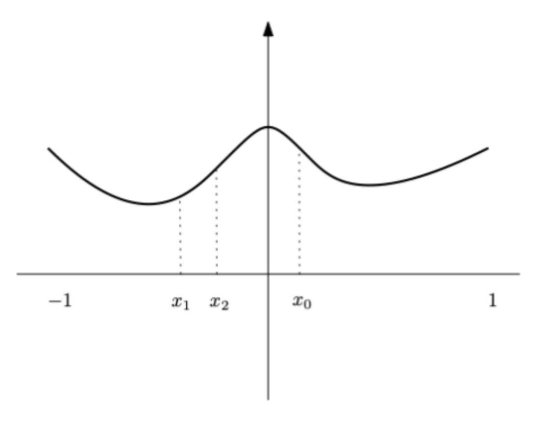
Welche der folgenden Aussagen gilt?
- Die Funktion \(f\) besitzt ein lokales Maximum in \(0\).
- \(f'(x_0) > 0\).
- \(f'(x_1) = 0\).
- \(f'(x_2) < 0\).
Back
ETH::2._Semester::Analysis::5._Differentialrechnung::5._Extremalstellen ETH::2._Semester::Analysis::Serie::9
Sei \(f : [-1, 1] \rightarrow \mathbb{R}\) eine Funktion mit folgendem Graphen:
Welche der folgenden Aussagen gilt?
- Die Funktion \(f\) besitzt ein lokales Maximum in \(0\).
- \(f'(x_0) > 0\).
- \(f'(x_1) = 0\).
- \(f'(x_2) < 0\).
(a) Die Funktion besitzt ein lokales Maximum in \(0\), da die Funktionswerte in einer Umgebung von \(0\) nicht grösser als \(f(0)\) sind.
(b), (c), (d) stimmen nicht mit den im Graphen dargestellten Steigungen bei \(x_0, x_1, x_2\) überein.
Field-by-field Comparison
| Field |
Before |
After |
| Front |
|
Sei \(f : [-1, 1] \rightarrow \mathbb{R}\) eine Funktion mit folgendem Graphen:<br><br><img src="paste-2cbb3f425e41341f58daf160517e99a355da6e17.jpg"><br><br>Welche der folgenden Aussagen gilt?<ol type="a"><li>Die Funktion \(f\) besitzt ein lokales Maximum in \(0\).</li><li>\(f'(x_0) > 0\).</li><li>\(f'(x_1) = 0\).</li><li>\(f'(x_2) < 0\).</li></ol> |
| Back |
|
<b>(a)</b> Die Funktion besitzt ein lokales Maximum in \(0\), da die Funktionswerte in einer Umgebung von \(0\) nicht grösser als \(f(0)\) sind.<br><br>(b), (c), (d) stimmen nicht mit den im Graphen dargestellten Steigungen bei \(x_0, x_1, x_2\) überein. |
Tags:
ETH::2._Semester::Analysis::5._Differentialrechnung::5._Extremalstellen
ETH::2._Semester::Analysis::Serie::9
Note 117: ETH::2. Semester::Analysis
Deck: ETH::2. Semester::Analysis
Note Type: Horvath Classic
GUID: zm(7{>{)@2
added
Previous
Note did not exist
New Note
Front
ETH::2._Semester::Analysis::6._Differentialgleichungen::2._Lineare_homogene::2._Lösungsstruktur ETH::2._Semester::Analysis::Serie::11
Es geht erneut um die lineare DGl \(u^{(n)} + a_{n-1} u^{(n-1)} + \dots + a_1 u' + a_0 u = b\) (L) mit Inhomogenität \(b \neq 0\) und die zugehörige homogene Gleichung (H). Entscheiden Sie: Sind \(u_1\) und \(u_2\) Lösungen von (L), so ist \(u_1 - u_2\) eine Lösung von (H).
- Richtig.
- Falsch.
Back
ETH::2._Semester::Analysis::6._Differentialgleichungen::2._Lineare_homogene::2._Lösungsstruktur ETH::2._Semester::Analysis::Serie::11
Es geht erneut um die lineare DGl \(u^{(n)} + a_{n-1} u^{(n-1)} + \dots + a_1 u' + a_0 u = b\) (L) mit Inhomogenität \(b \neq 0\) und die zugehörige homogene Gleichung (H). Entscheiden Sie: Sind \(u_1\) und \(u_2\) Lösungen von (L), so ist \(u_1 - u_2\) eine Lösung von (H).
- Richtig.
- Falsch.
(a) Richtig. Für \(v = u_1 - u_2\) gilt dank Linearität des Operators \(v^{(n)} + a_{n-1} v^{(n-1)} + \dots + a_0 v = b - b = 0\), also löst \(v\) die homogene Gleichung (H).
Field-by-field Comparison
| Field |
Before |
After |
| Front |
|
Es geht erneut um die lineare DGl \(u^{(n)} + a_{n-1} u^{(n-1)} + \dots + a_1 u' + a_0 u = b\) (L) mit Inhomogenität \(b \neq 0\) und die zugehörige homogene Gleichung (H). Entscheiden Sie: Sind \(u_1\) und \(u_2\) Lösungen von (L), so ist \(u_1 - u_2\) eine Lösung von (H).<ol type="a"><li>Richtig.</li><li>Falsch.</li></ol> |
| Back |
|
<b>(a)</b> Richtig. Für \(v = u_1 - u_2\) gilt dank Linearität des Operators \(v^{(n)} + a_{n-1} v^{(n-1)} + \dots + a_0 v = b - b = 0\), also löst \(v\) die homogene Gleichung (H). |
Tags:
ETH::2._Semester::Analysis::6._Differentialgleichungen::2._Lineare_homogene::2._Lösungsstruktur
ETH::2._Semester::Analysis::Serie::11
Note 118: ETH::2. Semester::Analysis
Deck: ETH::2. Semester::Analysis
Note Type: Horvath Cloze
GUID: ~cOVA$E|#n
added
Previous
Note did not exist
New Note
Front
ETH::2._Semester::Analysis::6._Differentialgleichungen::3._Lösungstechniken_erster_Ordnung::1._Trennung_der_Variablen
Trennung der Variablen
Grundidee: alle Ausdrücke mit der unabhängigen Variablen auf die eine Seite, alle Ausdrücke mit der abhängigen Variablen auf die andere Seite bringen, anschliessend beide Seiten (unbestimmt) integrieren.
Back
ETH::2._Semester::Analysis::6._Differentialgleichungen::3._Lösungstechniken_erster_Ordnung::1._Trennung_der_Variablen
Trennung der Variablen
Grundidee: alle Ausdrücke mit der unabhängigen Variablen auf die eine Seite, alle Ausdrücke mit der abhängigen Variablen auf die andere Seite bringen, anschliessend beide Seiten (unbestimmt) integrieren.
Das Verfahren eignet sich besonders für DGl der Form \(y'(x) = f(x) \cdot g(y)\).
Field-by-field Comparison
| Field |
Before |
After |
| Text |
|
<b>Trennung der Variablen</b><br>Grundidee: {{c1::alle Ausdrücke mit der unabhängigen Variablen auf die eine Seite, alle Ausdrücke mit der abhängigen Variablen auf die andere Seite bringen}}, anschliessend {{c2::beide Seiten (unbestimmt) integrieren}}. |
| Extra |
|
Das Verfahren eignet sich besonders für DGl der Form \(y'(x) = f(x) \cdot g(y)\). |
Tags:
ETH::2._Semester::Analysis::6._Differentialgleichungen::3._Lösungstechniken_erster_Ordnung::1._Trennung_der_Variablen
Note 119: ETH::2. Semester::PProg
Deck: ETH::2. Semester::PProg
Note Type: Horvath Cloze
GUID: !2-t6@qP8z
added
Previous
Note did not exist
New Note
Front
ETH::2._Semester::PProg::12._Linearizability_and_TM::4._Consensus
Atomic registers have consensus number 1.
Corollary: there is no wait-free implementation of n-thread consensus with \(n > 1\) from read-write registers.
Back
ETH::2._Semester::PProg::12._Linearizability_and_TM::4._Consensus
Atomic registers have consensus number 1.
Corollary: there is no wait-free implementation of n-thread consensus with \(n > 1\) from read-write registers.
With plain atomic read/write registers, not even two threads can reach consensus wait-free. This is the starting point for impossibility proofs (e.g. wait-free FIFO queue from registers).
Field-by-field Comparison
| Field |
Before |
After |
| Text |
|
Atomic registers have consensus number {{c1::1}}. <br><br>Corollary: {{c2::there is no wait-free implementation of n-thread consensus with \(n > 1\) from read-write registers}}. |
| Extra |
|
With plain atomic read/write registers, not even two threads can reach consensus wait-free. This is the starting point for impossibility proofs (e.g. wait-free FIFO queue from registers). |
Tags:
ETH::2._Semester::PProg::12._Linearizability_and_TM::4._Consensus
Note 120: ETH::2. Semester::PProg
Deck: ETH::2. Semester::PProg
Note Type: Horvath Cloze
GUID: !gF?S8.igA
modified
Before
Front
ETH::2._Semester::PProg::12._Shared_Memory_Concurrency::16._Lock-Free_Programming::4._Lock-Free_Queue
Final Michael-Scott
dequeue:
while (true) {
  Node first = head.get();
  Node last  = tail.get();
  Node next  = first.next.get();
  if (first == last) {
    if (next == null) return null;          // truly empty
    else tail.compareAndSet(last, next);    // help advance tail
  } else {
    T value = next.item;
    if (head.compareAndSet(first, next))
      return value;
  }
}
The two relevant cases when
first == last:
next == null means the queue is genuinely empty, return null;
next != null means an enqueue is in progress and tail lags; help advance it, then retry.
Back
ETH::2._Semester::PProg::12._Shared_Memory_Concurrency::16._Lock-Free_Programming::4._Lock-Free_Queue
Final Michael-Scott
dequeue:
while (true) {
  Node first = head.get();
  Node last  = tail.get();
  Node next  = first.next.get();
  if (first == last) {
    if (next == null) return null;          // truly empty
    else tail.compareAndSet(last, next);    // help advance tail
  } else {
    T value = next.item;
    if (head.compareAndSet(first, next))
      return value;
  }
}
The two relevant cases when
first == last:
next == null means the queue is genuinely empty, return null;
next != null means an enqueue is in progress and tail lags; help advance it, then retry.
Reading tail before first.next is what catches the inconsistency from the empty-queue enqueue scenario: if tail still equals first but first.next != null, the queue is in the half-enqueued state.
After
Front
ETH::2._Semester::PProg::11._Lock_Free_Programming::4._Lock_Free_Queue
Final Michael-Scott
dequeue:
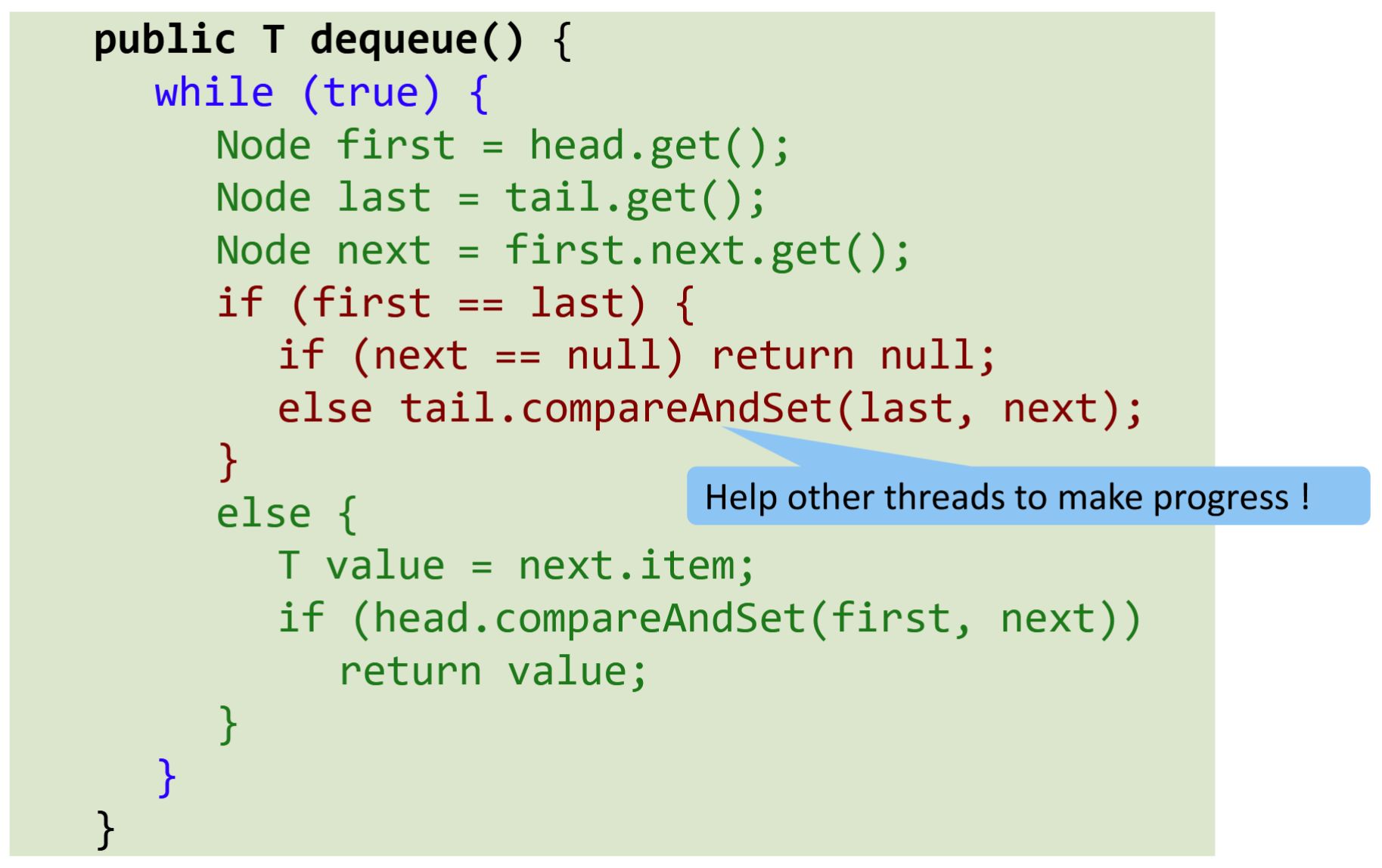
The two relevant cases when
first == last:
next == null means the queue is genuinely empty, return null; next != null means an enqueue is in progress and tail lags; help advance it, then retry.
Back
ETH::2._Semester::PProg::11._Lock_Free_Programming::4._Lock_Free_Queue
Final Michael-Scott
dequeue:
The two relevant cases when
first == last:
next == null means the queue is genuinely empty, return null; next != null means an enqueue is in progress and tail lags; help advance it, then retry.
Reading tail before first.next is what catches the inconsistency from the empty-queue enqueue scenario: if tail still equals first but first.next != null, the queue is in the half-enqueued state.
Field-by-field Comparison
| Field |
Before |
After |
| Text |
Final Michael-Scott <code>dequeue</code>: <pre>while (true) {
Node first = head.get();
Node last = tail.get();
Node next = first.next.get();
if (first == last) {
if (next == null) return null; // truly empty
else tail.compareAndSet(last, next); // help advance tail
} else {
T value = next.item;
if (head.compareAndSet(first, next))
return value;
}
}</pre> The two relevant cases when <code>first == last</code>: {{c1::<code>next == null</code> means the queue is genuinely empty, return <code>null</code>}}; {{c2::<code>next != null</code> means an enqueue is in progress and <code>tail</code> lags; help advance it, then retry}}. |
Final Michael-Scott <code>dequeue</code>: <br><br><img src="paste-e3369744e483694f7194dffe6053043775493aef.jpg"><br><br>The two relevant cases when <code>first == last</code>: <br><ol><li>{{c1::<code>next == null</code> means the queue is genuinely empty, return <code>null</code>}}; </li><li>{{c2::<code>next != null</code> means an enqueue is in progress and <code>tail</code> lags; help advance it, then retry}}.</li></ol> |
Tags:
ETH::2._Semester::PProg::12._Shared_Memory_Concurrency::16._Lock-Free_Programming::4._Lock-Free_Queue
ETH::2._Semester::PProg::11._Lock_Free_Programming::4._Lock_Free_Queue
Note 121: ETH::2. Semester::PProg
Deck: ETH::2. Semester::PProg
Note Type: Horvath Cloze
GUID: !rbAr}u{}v
added
Previous
Note did not exist
New Note
Front
ETH::2._Semester::PProg::12._Linearizability_and_TM::5._Transactional_Memory_Motivation
Two further lock problems:
- Locks are pessimistic, i.e. the worst is assumed and the performance overhead is paid every time.
- Also, the locking mechanism is hard-wired into the program: synchronisation and the rest of the program cannot be separated, and changing the synchronisation scheme means changing the whole program.
Back
ETH::2._Semester::PProg::12._Linearizability_and_TM::5._Transactional_Memory_Motivation
Two further lock problems:
- Locks are pessimistic, i.e. the worst is assumed and the performance overhead is paid every time.
- Also, the locking mechanism is hard-wired into the program: synchronisation and the rest of the program cannot be separated, and changing the synchronisation scheme means changing the whole program.
TM, by contrast, is optimistic by design and separates the what from the how.
Field-by-field Comparison
| Field |
Before |
After |
| Text |
|
Two further lock problems: <br><ol><li>Locks are {{c1::pessimistic, i.e. the worst is assumed and the performance overhead is paid every time}}. </li><li>Also, the locking mechanism is {{c2::hard-wired into the program: synchronisation and the rest of the program cannot be separated, and changing the synchronisation scheme means changing the whole program}}.</li></ol> |
| Extra |
|
TM, by contrast, is optimistic by design and separates the what from the how. |
Tags:
ETH::2._Semester::PProg::12._Linearizability_and_TM::5._Transactional_Memory_Motivation
Note 122: ETH::2. Semester::PProg
Deck: ETH::2. Semester::PProg
Note Type: Horvath Cloze
GUID: $]0GJ@6n0.
added
Previous
Note did not exist
New Note
Front
ETH::2._Semester::PProg::12._Linearizability_and_TM::3._Consistency_Models
Composability theorem (locality):
A history \(H\) is linearizable if and only if
for every object \(x\) the projection \(H\,|\,x\) is linearizable.
Consequence for modularity:
- linearizability of individual objects can be proved in isolation, and
- independently implemented objects can be composed without losing linearizability.
Back
ETH::2._Semester::PProg::12._Linearizability_and_TM::3._Consistency_Models
Composability theorem (locality):
A history \(H\) is linearizable if and only if
for every object \(x\) the projection \(H\,|\,x\) is linearizable.
Consequence for modularity:
- linearizability of individual objects can be proved in isolation, and
- independently implemented objects can be composed without losing linearizability.
Linearizability is a local property: the correctness of the whole system follows from the correctness of the individual objects. This is exactly the property that sequential consistency lacks.
Field-by-field Comparison
| Field |
Before |
After |
| Text |
|
Composability theorem (locality): <br><br>A history \(H\) is linearizable if and only if {{c1::for every object \(x\) the projection \(H\,|\,x\) is linearizable}}. <br><br>Consequence for modularity: <br><ol><li>{{c2::linearizability of individual objects can be proved in isolation}}, and </li><li>{{c2::independently implemented objects can be composed without losing linearizability}}.</li></ol> |
| Extra |
|
Linearizability is a local property: the correctness of the whole system follows from the correctness of the individual objects. This is exactly the property that sequential consistency lacks. |
Tags:
ETH::2._Semester::PProg::12._Linearizability_and_TM::3._Consistency_Models
Note 123: ETH::2. Semester::PProg
Deck: ETH::2. Semester::PProg
Note Type: Horvath Cloze
GUID: $zyCmI+(er
added
Previous
Note did not exist
New Note
Front
ETH::2._Semester::PProg::12._Linearizability_and_TM::7._Conflicts_and_Implementation
Software TM (STM): implemented in the (parallel) programming language, offers greater flexibility, but achieving good performance can be challenging. Examples: Haskell, Clojure. Hybrid TM (hardware + software) is currently a research topic.
Back
ETH::2._Semester::PProg::12._Linearizability_and_TM::7._Conflicts_and_Implementation
Software TM (STM): implemented in the (parallel) programming language, offers greater flexibility, but achieving good performance can be challenging. Examples: Haskell, Clojure. Hybrid TM (hardware + software) is currently a research topic.
STM implementations are still actively developed, whereas pure HTM (RTM) barely succeeded in the market. Overall, TM is still work in progress.
Field-by-field Comparison
| Field |
Before |
After |
| Text |
|
Software TM (STM): implemented in the (parallel) programming language, offers {{c1::greater flexibility}}, but {{c2::achieving good performance can be challenging}}. Examples: Haskell, Clojure. Hybrid TM (hardware + software) is currently a {{c3::research topic}}. |
| Extra |
|
STM implementations are still actively developed, whereas pure HTM (RTM) barely succeeded in the market. Overall, TM is still work in progress. |
Tags:
ETH::2._Semester::PProg::12._Linearizability_and_TM::7._Conflicts_and_Implementation
Note 124: ETH::2. Semester::PProg
Deck: ETH::2. Semester::PProg
Note Type: Horvath Cloze
GUID: %O}~X:[ObV
added
Previous
Note did not exist
New Note
Front
ETH::2._Semester::PProg::12._Linearizability_and_TM::2._Histories
Two projections of a history \(H\):
- the object projection \(H\,|\,q\) keeps only events whose object is \(q\);
- the thread projection \(H\,|\,B\) keeps only events whose thread is \(B\).
Back
ETH::2._Semester::PProg::12._Linearizability_and_TM::2._Histories
Two projections of a history \(H\):
- the object projection \(H\,|\,q\) keeps only events whose object is \(q\);
- the thread projection \(H\,|\,B\) keeps only events whose thread is \(B\).
Projections are the basic slicing operation used to define well-formedness, equivalence and legality.
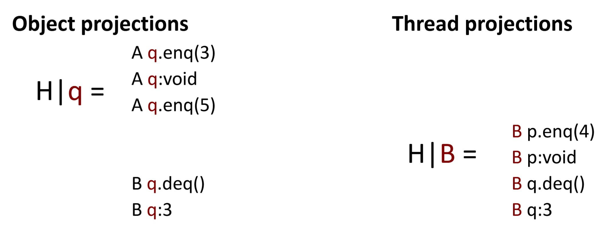
Field-by-field Comparison
| Field |
Before |
After |
| Text |
|
Two projections of a history \(H\): <ul><li>the object projection {{c1::\(H\,|\,q\)}} keeps only events whose object is \(q\);</li><li>the thread projection {{c1::\(H\,|\,B\)}} keeps only events whose thread is \(B\).</li></ul> |
| Extra |
|
Projections are the basic slicing operation used to define well-formedness, equivalence and legality.<br><br><img src="paste-419f30bdb53ec3843bcb9b486d3977092c0e7e98.jpg"> |
Tags:
ETH::2._Semester::PProg::12._Linearizability_and_TM::2._Histories
Note 125: ETH::2. Semester::PProg
Deck: ETH::2. Semester::PProg
Note Type: Horvath Cloze
GUID: ){3bJVnlBC
added
Previous
Note did not exist
New Note
Front
ETH::2._Semester::PProg::12._Linearizability_and_TM::4._Consensus
Consensus numbers at a glance:
- wait-free FIFO queues have consensus number 2;
- Test-And-Set, getAndSet and getAndIncrement have consensus number 2;
- Compare-And-Swap has consensus number \(\infty\).
It follows that wait-free FIFO queues, wait-free RMW operations and CAS
cannot be implemented from atomic registers.
Back
ETH::2._Semester::PProg::12._Linearizability_and_TM::4._Consensus
Consensus numbers at a glance:
- wait-free FIFO queues have consensus number 2;
- Test-And-Set, getAndSet and getAndIncrement have consensus number 2;
- Compare-And-Swap has consensus number \(\infty\).
It follows that wait-free FIFO queues, wait-free RMW operations and CAS
cannot be implemented from atomic registers.
This also answers the opening question of why CAS is more powerful than TAS:
TAS only solves 2-thread consensus, whereas CAS solves n-thread consensus for arbitrary \(n\).
Field-by-field Comparison
| Field |
Before |
After |
| Text |
|
Consensus numbers at a glance: <br><ol><li>wait-free FIFO queues have consensus number {{c1::2}}; </li><li>Test-And-Set, getAndSet and getAndIncrement have consensus number {{c2::2}}; </li><li>Compare-And-Swap has consensus number {{c3::\(\infty\)}}. </li></ol>It follows that wait-free FIFO queues, wait-free RMW operations and CAS {{c4::cannot be implemented from atomic registers}}.<br> |
| Extra |
|
This also answers the opening question of why CAS is more powerful than TAS: <br>TAS only solves 2-thread consensus, whereas CAS solves n-thread consensus for arbitrary \(n\). |
Tags:
ETH::2._Semester::PProg::12._Linearizability_and_TM::4._Consensus
Note 126: ETH::2. Semester::PProg
Deck: ETH::2. Semester::PProg
Note Type: Horvath Cloze
GUID: *7_xp,WYW>
added
Previous
Note did not exist
New Note
Front
ETH::2._Semester::PProg::12._Linearizability_and_TM::6._Transactional_Memory_Semantics
TM semantics, atomicity:
The changes made by a transaction are made visible atomically (all at once); other threads see either the initial state or the final state, but no intermediate states.
Difference from locks:
Locks enforce atomicity via mutual exclusion, whereas transactions do not require mutual exclusion.
Back
ETH::2._Semester::PProg::12._Linearizability_and_TM::6._Transactional_Memory_Semantics
TM semantics, atomicity:
The changes made by a transaction are made visible atomically (all at once); other threads see either the initial state or the final state, but no intermediate states.
Difference from locks:
Locks enforce atomicity via mutual exclusion, whereas transactions do not require mutual exclusion.
Atomicity here is an all-or-nothing visibility to the outside, not a mechanism.
Field-by-field Comparison
| Field |
Before |
After |
| Text |
|
TM semantics, atomicity: <br>The changes made by a transaction are {{c1::made visible atomically (all at once)}}; other threads see either {{c1::the initial state or the final state, but no intermediate states}}. <br><br>Difference from locks: <br>Locks enforce atomicity via {{c2::mutual exclusion}}, whereas transactions {{c2::do not require mutual exclusion}}. |
| Extra |
|
Atomicity here is an all-or-nothing visibility to the outside, not a mechanism. |
Tags:
ETH::2._Semester::PProg::12._Linearizability_and_TM::6._Transactional_Memory_Semantics
Note 127: ETH::2. Semester::PProg
Deck: ETH::2. Semester::PProg
Note Type: Horvath Cloze
GUID: *TqZbFEvYt
added
Previous
Note did not exist
New Note
Front
ETH::2._Semester::PProg::12._Linearizability_and_TM::4._Consensus
A consensus object offers the operation
T decide(T value): several threads call
c.decide(v), each with one input value.
A consensus protocol must satisfy three requirements:
- wait-free (each thread terminates in finite time),
- consistent (all threads decide the same value), and
- valid (the common decision value is the input of some thread).
Back
ETH::2._Semester::PProg::12._Linearizability_and_TM::4._Consensus
A consensus object offers the operation
T decide(T value): several threads call
c.decide(v), each with one input value.
A consensus protocol must satisfy three requirements:
- wait-free (each thread terminates in finite time),
- consistent (all threads decide the same value), and
- valid (the common decision value is the input of some thread).
Linearizability enforces that the decision of the first thread is adopted by all. Validity forbids deciding a value that nobody proposed.
Field-by-field Comparison
| Field |
Before |
After |
| Text |
|
A consensus object offers the operation <code>T decide(T value)</code>: several threads call <code>c.decide(v)</code>, each with one input value. <br><br>A consensus protocol must satisfy three requirements: <br><ol><li>{{c1::wait-free (each thread terminates in finite time)}}, </li><li>{{c2::consistent (all threads decide the same value)}}, and </li><li>{{c3::valid (the common decision value is the input of some thread)}}.</li></ol> |
| Extra |
|
Linearizability enforces that the decision of the first thread is adopted by all. Validity forbids deciding a value that nobody proposed. |
Tags:
ETH::2._Semester::PProg::12._Linearizability_and_TM::4._Consensus
Note 128: ETH::2. Semester::PProg
Deck: ETH::2. Semester::PProg
Note Type: Horvath Cloze
GUID: +QfX%F6A5H
added
Previous
Note did not exist
New Note
Front
ETH::2._Semester::PProg::11._Lock_Free_Programming::6._Hazard_Pointers
The ABA problem also affects the node pool itself. Three remedies:
- thread-local node pools: no protection needed, but they fail when push/pop are not well balanced (one thread leaks, another starves);
- hazard pointers on the global pool: expensive on reuse, equivalent to the code above (the pool returns a node only when it is not hazardous);
- a hybrid: thread-local pool plus a global pool guarded by hazard pointers.
Back
ETH::2._Semester::PProg::11._Lock_Free_Programming::6._Hazard_Pointers
The ABA problem also affects the node pool itself. Three remedies:
- thread-local node pools: no protection needed, but they fail when push/pop are not well balanced (one thread leaks, another starves);
- hazard pointers on the global pool: expensive on reuse, equivalent to the code above (the pool returns a node only when it is not hazardous);
- a hybrid: thread-local pool plus a global pool guarded by hazard pointers.
Thread-local storage avoids contention entirely but is unsafe under imbalance; the hybrid captures the best of both.
Field-by-field Comparison
| Field |
Before |
After |
| Text |
|
The ABA problem also affects the node pool itself. Three remedies: <ul><li>{{c1::thread-local node pools: no protection needed, but they fail when push/pop are not well balanced (one thread leaks, another starves)}};</li><li>{{c2::hazard pointers on the global pool: expensive on reuse, equivalent to the code above (the pool returns a node only when it is not hazardous)}};</li><li>{{c3::a hybrid: thread-local pool plus a global pool guarded by hazard pointers}}.</li></ul> |
| Extra |
|
Thread-local storage avoids contention entirely but is unsafe under imbalance; the hybrid captures the best of both. |
Tags:
ETH::2._Semester::PProg::11._Lock_Free_Programming::6._Hazard_Pointers
Note 129: ETH::2. Semester::PProg
Deck: ETH::2. Semester::PProg
Note Type: Horvath Cloze
GUID: ,NDJ
modified
Before
Front
ETH::2._Semester::PProg::12._Shared_Memory_Concurrency::16._Lock-Free_Programming::5._ABA_Problem
Concrete ABA scenario on a CAS-based stack with a node pool. Thread X starts pop, reads head = A and next = A.next, then stalls before its CAS. While X is paused: Y pops A (so A goes back into the pool); Z pushes B (now top = B → ... ); Z' pushes A again (recycled from the pool; top = A → B → ...). X now wakes up and runs top.compareAndSet(A, A.next_old). The CAS succeeds because top is again A, but it now points top at a stale successor, corrupting the stack.
Back
ETH::2._Semester::PProg::12._Shared_Memory_Concurrency::16._Lock-Free_Programming::5._ABA_Problem
Concrete ABA scenario on a CAS-based stack with a node pool. Thread X starts pop, reads head = A and next = A.next, then stalls before its CAS. While X is paused: Y pops A (so A goes back into the pool); Z pushes B (now top = B → ... ); Z' pushes A again (recycled from the pool; top = A → B → ...). X now wakes up and runs top.compareAndSet(A, A.next_old). The CAS succeeds because top is again A, but it now points top at a stale successor, corrupting the stack.
The corruption is observable as the symptoms in the lecture's runs: "sum of pushes and pops don't match" (lost items) or an infinite hang (lost node forms a self-cycle). Crucially, this cannot happen without reuse: a freshly allocated node has a brand-new identity, so the CAS would fail.
After
Front
ETH::2._Semester::PProg::11._Lock_Free_Programming::5._ABA_Problem
Concrete ABA scenario on a CAS-based stack with a node pool.
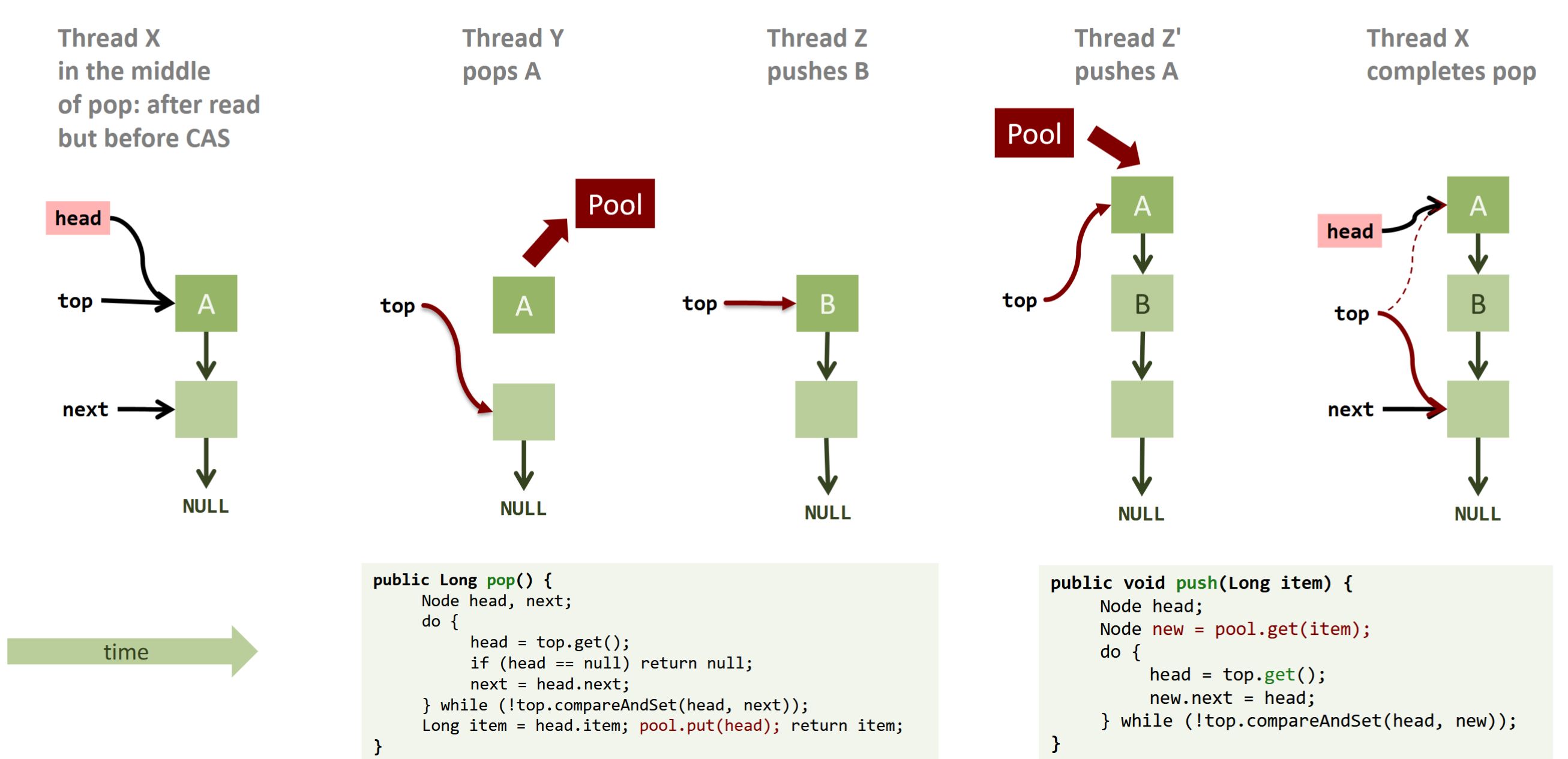
Thread X starts
pop, reads
head = A and
next = A.next, then stalls before its CAS.
While X is paused:
- Y pops A (so A goes back into the pool);
- Z pushes B (now top = B → ... );
- Z' pushes A again (recycled from the pool; top = A → B → ...).
X now wakes up and runs
top.compareAndSet(A, A.next_old).
The CAS
succeeds because top is again A, but it now points top at a stale successor, corrupting the stack.
Back
ETH::2._Semester::PProg::11._Lock_Free_Programming::5._ABA_Problem
Concrete ABA scenario on a CAS-based stack with a node pool.
Thread X starts
pop, reads
head = A and
next = A.next, then stalls before its CAS.
While X is paused:
- Y pops A (so A goes back into the pool);
- Z pushes B (now top = B → ... );
- Z' pushes A again (recycled from the pool; top = A → B → ...).
X now wakes up and runs
top.compareAndSet(A, A.next_old).
The CAS
succeeds because top is again A, but it now points top at a stale successor, corrupting the stack.
The corruption is observable as the symptoms in the lecture's runs: "sum of pushes and pops don't match" (lost items) or an infinite hang (lost node forms a self-cycle). Crucially, this cannot happen without reuse: a freshly allocated node has a brand-new identity, so the CAS would fail.
Field-by-field Comparison
| Field |
Before |
After |
| Text |
Concrete ABA scenario on a CAS-based stack with a node pool. Thread X starts <code>pop</code>, reads <code>head = A</code> and <code>next = A.next</code>, then stalls before its CAS. While X is paused: {{c1::Y pops A (so A goes back into the pool)}}; {{c2::Z pushes B (now top = B → ... )}}; {{c3::Z' pushes A again (recycled from the pool; top = A → B → ...)}}. X now wakes up and runs <code>top.compareAndSet(A, A.next_old)</code>. The CAS {{c4::succeeds because top is again <code>A</code>, but it now points <code>top</code> at a stale successor, corrupting the stack}}. |
Concrete ABA scenario on a CAS-based stack with a node pool. <br><br><img src="paste-7de67200e092a2e2094825997c124cb439e9dfc7.jpg"><br><br>Thread X starts <code>pop</code>, reads <code>head = A</code> and <code>next = A.next</code>, then stalls before its CAS. <br><br>While X is paused: <br><ol><li>Y pops A (so A goes back into the pool); </li><li>Z pushes B (now top = B → ... ); </li><li>Z' pushes A again (recycled from the pool; top = A → B → ...). </li></ol>X now wakes up and runs <code>top.compareAndSet(A, A.next_old)</code>. <br><br>The CAS {{c1::succeeds because top is again <code>A</code>, but it now points <code>top</code> at a stale successor, corrupting the stack}}.<br> |
Tags:
ETH::2._Semester::PProg::12._Shared_Memory_Concurrency::16._Lock-Free_Programming::5._ABA_Problem
ETH::2._Semester::PProg::11._Lock_Free_Programming::5._ABA_Problem
Note 130: ETH::2. Semester::PProg
Deck: ETH::2. Semester::PProg
Note Type: Horvath Cloze
GUID: -GMd8PbbE3
added
Previous
Note did not exist
New Note
Front
ETH::2._Semester::PProg::12._Linearizability_and_TM::3._Consistency_Models
Sequential consistency is not a local property, and consequently not composable (not modular).
Proof idea (FIFO queues \(p\) and \(q\)):
There is a history \(H\) in which both \(H\,|\,p\) and \(H\,|\,q\) are sequentially consistent on their own, but the orders forced by \(H\,|\,p\) and \(H\,|\,q\) together are cyclic, so that \(H\) as a whole is not sequentially consistent.
Back
ETH::2._Semester::PProg::12._Linearizability_and_TM::3._Consistency_Models
Sequential consistency is not a local property, and consequently not composable (not modular).
Proof idea (FIFO queues \(p\) and \(q\)):
There is a history \(H\) in which both \(H\,|\,p\) and \(H\,|\,q\) are sequentially consistent on their own, but the orders forced by \(H\,|\,p\) and \(H\,|\,q\) together are cyclic, so that \(H\) as a whole is not sequentially consistent.
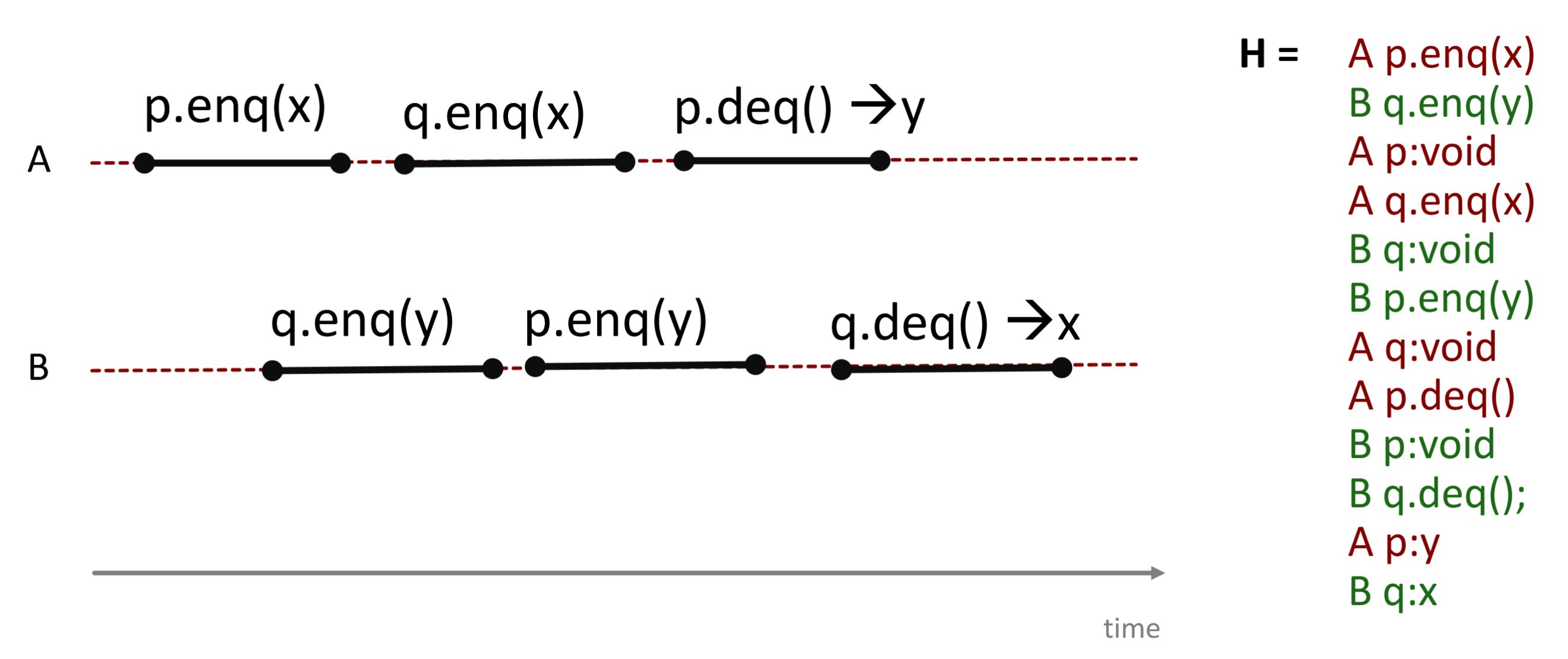
Thus sequential consistency is weaker than linearizability exactly where it matters: you cannot verify objects in isolation and then compose them carelessly. The same statement holds for the flags example (two registers \(x\), \(y\)): each single projection is SC, the whole is not.
Field-by-field Comparison
| Field |
Before |
After |
| Text |
|
Sequential consistency is {{c1::not a local property}}, and consequently {{c2::not composable (not modular)}}. <br><br>Proof idea (FIFO queues \(p\) and \(q\)): <br>There is a history \(H\) in which {{c3::both \(H\,|\,p\) and \(H\,|\,q\) are sequentially consistent on their own, but the orders forced by \(H\,|\,p\) and \(H\,|\,q\) together are cyclic}}, so that \(H\) as a whole is not sequentially consistent. |
| Extra |
|
<img src="paste-101c15f85be3572a0a3c2db69b701b2af6588e81.jpg"><br><br>Thus sequential consistency is weaker than linearizability exactly where it matters: you cannot verify objects in isolation and then compose them carelessly. The same statement holds for the flags example (two registers \(x\), \(y\)): each single projection is SC, the whole is not. |
Tags:
ETH::2._Semester::PProg::12._Linearizability_and_TM::3._Consistency_Models
Note 131: ETH::2. Semester::PProg
Deck: ETH::2. Semester::PProg
Note Type: Horvath Cloze
GUID: -OZfQ3)e,*
added
Previous
Note did not exist
New Note
Front
ETH::2._Semester::PProg::12._Linearizability_and_TM::6._Transactional_Memory_Semantics
Serializability:
Concurrently executed transactions behave as if they had been executed sequentially, one after another, in some serial order.
The transactions appear serialized without actually running serially.
Back
ETH::2._Semester::PProg::12._Linearizability_and_TM::6._Transactional_Memory_Semantics
Serializability:
Concurrently executed transactions behave as if they had been executed sequentially, one after another, in some serial order.
The transactions appear serialized without actually running serially.
Example: if TXA and TXB run concurrently, a valid outcome is one that would also arise from the serial order TXB then TXA (or TXA then TXB).
Field-by-field Comparison
| Field |
Before |
After |
| Text |
|
Serializability: <br><br>Concurrently executed transactions behave {{c1::as if they had been executed sequentially, one after another, in some serial order}}. <br><br>The transactions {{c2::appear serialized}} without actually running serially. |
| Extra |
|
Example: if TXA and TXB run concurrently, a valid outcome is one that would also arise from the serial order TXB then TXA (or TXA then TXB). |
Tags:
ETH::2._Semester::PProg::12._Linearizability_and_TM::6._Transactional_Memory_Semantics
Note 132: ETH::2. Semester::PProg
Deck: ETH::2. Semester::PProg
Note Type: Horvath Cloze
GUID: 0[Xp*HWVwd
added
Previous
Note did not exist
New Note
Front
ETH::2._Semester::PProg::12._Linearizability_and_TM::7._Conflicts_and_Implementation
Handling conflicts in TM: transactions are aborted if necessary. Such cases are handled by the concurrency-control (CC) mechanism. When a transaction aborts, it can be retried automatically, or the user is notified.
Back
ETH::2._Semester::PProg::12._Linearizability_and_TM::7._Conflicts_and_Implementation
Handling conflicts in TM: transactions are aborted if necessary. Such cases are handled by the concurrency-control (CC) mechanism. When a transaction aborts, it can be retried automatically, or the user is notified.
Field-by-field Comparison
| Field |
Before |
After |
| Text |
|
Handling conflicts in TM: transactions are {{c1::aborted}} if necessary. Such cases are handled by the {{c2::concurrency-control (CC) mechanism}}. When a transaction aborts, it can be {{c3::retried automatically, or the user is notified}}. |
Tags:
ETH::2._Semester::PProg::12._Linearizability_and_TM::7._Conflicts_and_Implementation
Note 133: ETH::2. Semester::PProg
Deck: ETH::2. Semester::PProg
Note Type: Horvath Cloze
GUID: 0q^f:9igUa
added
Previous
Note did not exist
New Note
Front
ETH::2._Semester::PProg::12._Linearizability_and_TM::6._Transactional_Memory_Semantics
TM is heavily inspired by database transactions.
The ACID properties are:
- Atomicity;
- Consistency (data remains in a consistent state);
- Isolation (no mutual corruption of data);
- Durability (effects survive e.g. power loss, because stored on disk).
Back
ETH::2._Semester::PProg::12._Linearizability_and_TM::6._Transactional_Memory_Semantics
TM is heavily inspired by database transactions.
The ACID properties are:
- Atomicity;
- Consistency (data remains in a consistent state);
- Isolation (no mutual corruption of data);
- Durability (effects survive e.g. power loss, because stored on disk).
Durability is the database-specific property and barely matters for in-memory TM; for TM mainly atomicity, consistency, and isolation count.
Field-by-field Comparison
| Field |
Before |
After |
| Text |
|
TM is heavily inspired by database transactions. <br><br>The ACID properties are: <br><ol><li>{{c1::Atomicity}}; </li><li>{{c2::Consistency (data remains in a consistent state)}}; </li><li>{{c3::Isolation (no mutual corruption of data)}}; </li><li>{{c4::Durability (effects survive e.g. power loss, because stored on disk)}}.</li></ol> |
| Extra |
|
Durability is the database-specific property and barely matters for in-memory TM; for TM mainly atomicity, consistency, and isolation count. |
Tags:
ETH::2._Semester::PProg::12._Linearizability_and_TM::6._Transactional_Memory_Semantics
Note 134: ETH::2. Semester::PProg
Deck: ETH::2. Semester::PProg
Note Type: Horvath Cloze
GUID: 24t~}WO)|v
added
Previous
Note did not exist
New Note
Front
ETH::2._Semester::PProg::12._Linearizability_and_TM::1._Linearizability
Sequential versus concurrent objects:
| Sequential | Concurrent |
|---|
| State is meaningful only between method calls. | Calls overlap; the object may never be between calls (except periods of quiescence). |
| Methods described in isolation. | All possible interactions with concurrent calls must be considered. |
| New methods can be added without affecting older ones. | Everything can interact with everything else. |
| Global clock. | Object/thread clock. |
Back
ETH::2._Semester::PProg::12._Linearizability_and_TM::1._Linearizability
Sequential versus concurrent objects:
| Sequential | Concurrent |
|---|
| State is meaningful only between method calls. | Calls overlap; the object may never be between calls (except periods of quiescence). |
| Methods described in isolation. | All possible interactions with concurrent calls must be considered. |
| New methods can be added without affecting older ones. | Everything can interact with everything else. |
| Global clock. | Object/thread clock. |
A period of quiescence is an interval with no pending calls; only then does a concurrent object have a well-defined sequential-style state.
Field-by-field Comparison
| Field |
Before |
After |
| Text |
|
Sequential versus concurrent objects: <br><br><table border="1" style="border-collapse:collapse"><tbody><tr><th>Sequential</th><th>Concurrent</th></tr><tr><td>State is meaningful only between method calls.</td><td>{{c1::Calls overlap; the object may never be between calls (except periods of quiescence)}}.</td></tr><tr><td>Methods described in isolation.</td><td>{{c2::All possible interactions with concurrent calls must be considered}}.</td></tr><tr><td>New methods can be added without affecting older ones.</td><td>{{c3::Everything can interact with everything else}}.</td></tr><tr><td>Global clock.</td><td>{{c4::Object/thread clock}}.</td></tr></tbody></table> |
| Extra |
|
A period of quiescence is an interval with no pending calls; only then does a concurrent object have a well-defined sequential-style state. |
Tags:
ETH::2._Semester::PProg::12._Linearizability_and_TM::1._Linearizability
Note 135: ETH::2. Semester::PProg
Deck: ETH::2. Semester::PProg
Note Type: Horvath Cloze
GUID: 3?nSJ.&XB-
added
Previous
Note did not exist
New Note
Front
ETH::2._Semester::PProg::12._Linearizability_and_TM::2._Histories
A history \(H\) is a sequence of invocation and response events.
Each event is written with its thread and object, e.g. invocation A q.enq(x) (thread, object, method, arguments) and response A q:void (thread, object, result).
An invocation and a response match if their thread names and object names agree.
Back
ETH::2._Semester::PProg::12._Linearizability_and_TM::2._Histories
A history \(H\) is a sequence of invocation and response events.
Each event is written with its thread and object, e.g. invocation A q.enq(x) (thread, object, method, arguments) and response A q:void (thread, object, result).
An invocation and a response match if their thread names and object names agree.
This split-into-events view is what lets us talk about overlapping calls precisely.
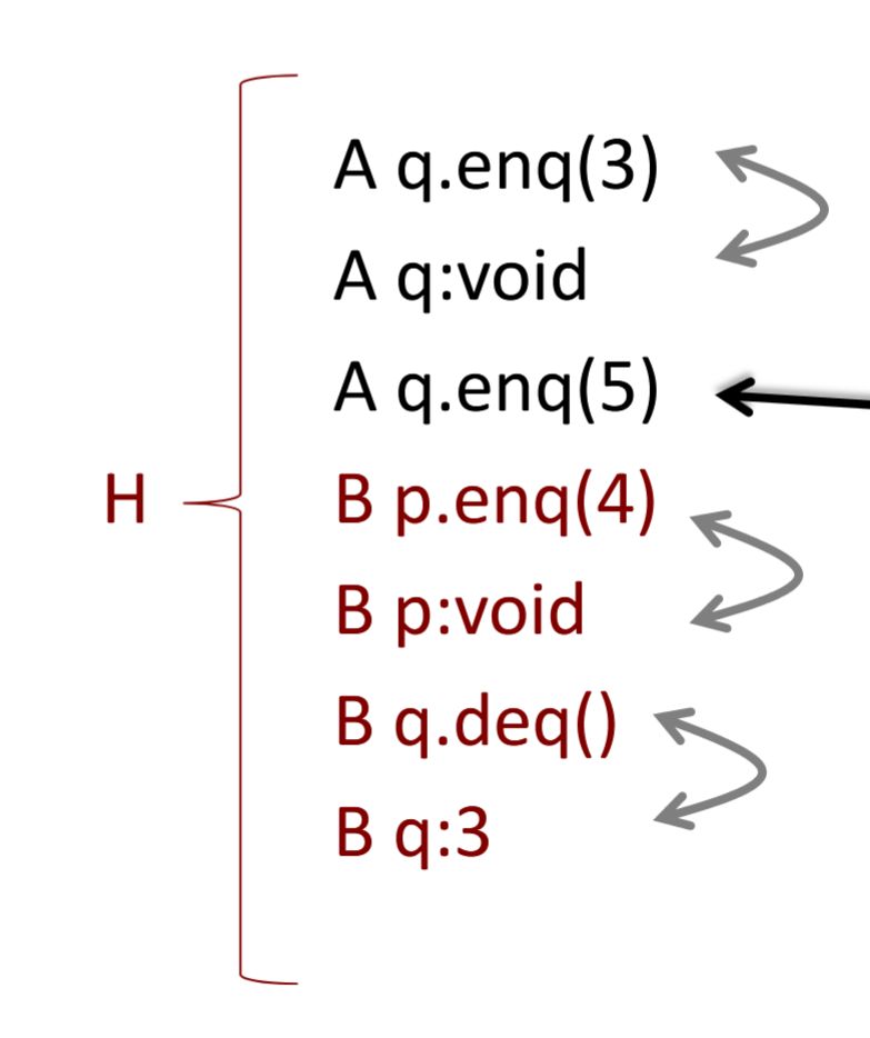
Field-by-field Comparison
| Field |
Before |
After |
| Text |
|
A history \(H\) is a {{c1::sequence of invocation and response events}}. <br><br>Each event is written with its thread and object, e.g. invocation <code>A q.enq(x)</code> (thread, object, method, arguments) and response <code>A q:void</code> (thread, object, result). <br><br>An invocation and a response match {{c2::if their thread names and object names agree}}. |
| Extra |
|
This split-into-events view is what lets us talk about overlapping calls precisely.<br><br><img src="paste-dbb1907c804d9cd6d138a8c67b50b4264399f11c.jpg"> |
Tags:
ETH::2._Semester::PProg::12._Linearizability_and_TM::2._Histories
Note 136: ETH::2. Semester::PProg
Deck: ETH::2. Semester::PProg
Note Type: Horvath Cloze
GUID: 5jCCKEp1WY
added
Previous
Note did not exist
New Note
Front
ETH::2._Semester::PProg::12._Linearizability_and_TM::7._Conflicts_and_Implementation
Zombies and consistency (initially a = 10, b = 0, c = 0): TXA computes c = 1 / (a-b), TXB commits with a = 0, b = 10. If TXA inconsistently read the already-committed b = 10 (but kept the old a), then a-b = 0, giving a division by zero (catastrophic inconsistency). Guarantee of the TM system: a running transaction is always shown consistent data. Conceptual possibilities: snapshot at the beginning or early abort.
Back
ETH::2._Semester::PProg::12._Linearizability_and_TM::7._Conflicts_and_Implementation
Zombies and consistency (initially a = 10, b = 0, c = 0): TXA computes c = 1 / (a-b), TXB commits with a = 0, b = 10. If TXA inconsistently read the already-committed b = 10 (but kept the old a), then a-b = 0, giving a division by zero (catastrophic inconsistency). Guarantee of the TM system: a running transaction is always shown consistent data. Conceptual possibilities: snapshot at the beginning or early abort.
A zombie is a doomed (later aborted) transaction that transiently sees inconsistent data. Without a consistency guarantee it could cause damage (e.g. crash, infinite loop) before it is even aborted.
Field-by-field Comparison
| Field |
Before |
After |
| Text |
|
Zombies and consistency (initially a = 10, b = 0, c = 0): TXA computes c = 1 / (a-b), TXB commits with a = 0, b = 10. If TXA inconsistently read the already-committed b = 10 (but kept the old a), then a-b = 0, giving a {{c1::division by zero (catastrophic inconsistency)}}. Guarantee of the TM system: a running transaction is always shown {{c2::consistent data}}. Conceptual possibilities: {{c3::snapshot at the beginning}} or {{c3::early abort}}. |
| Extra |
|
A zombie is a doomed (later aborted) transaction that transiently sees inconsistent data. Without a consistency guarantee it could cause damage (e.g. crash, infinite loop) before it is even aborted. |
Tags:
ETH::2._Semester::PProg::12._Linearizability_and_TM::7._Conflicts_and_Implementation
Note 137: ETH::2. Semester::PProg
Deck: ETH::2. Semester::PProg
Note Type: Horvath Classic
GUID: 6.;IeGU,Ik
added
Previous
Note did not exist
New Note
Front
ETH::2._Semester::PProg::12._Linearizability_and_TM::7._Conflicts_and_Implementation
What does the bank account look like in ScalaSTM (on Java), and why use new Runnable() instead of just atomic?
Back
ETH::2._Semester::PProg::12._Linearizability_and_TM::7._Conflicts_and_Implementation
What does the bank account look like in ScalaSTM (on Java), and why use new Runnable() instead of just atomic?
The mutable balance lives in a Ref:
class AccountSTM {
    private final Integer id;
    private final Ref.View<Integer> balance;
    AccountSTM(int id, int balance) {
        this.id = new Integer(id);
        this.balance = STM.newRef(balance);
    }
}
Ideal world with an atomic keyword:
void withdraw(final int amount) {
    atomic {
        int old_val = balance.get();
        balance.set(old_val - amount);
    }
}
Real ScalaSTM version (Java 7 has no lambdas), each transaction is a Runnable:
void withdraw(final int amount) {
    STM.atomic(new Runnable() { public void run() {
        int old_val = balance.get();
        balance.set(old_val - amount);
    }});
}
There is also no compiler support enforcing that Refs are only accessed inside a transaction.
Field-by-field Comparison
| Field |
Before |
After |
| Front |
|
What does the bank account look like in ScalaSTM (on Java), and why use new Runnable() instead of just atomic? |
| Back |
|
The mutable balance lives in a Ref: <pre>class AccountSTM {
private final Integer id;
private final Ref.View<Integer> balance;
AccountSTM(int id, int balance) {
this.id = new Integer(id);
this.balance = STM.newRef(balance);
}
}</pre>Ideal world with an atomic keyword: <pre>void withdraw(final int amount) {
atomic {
int old_val = balance.get();
balance.set(old_val - amount);
}
}</pre>Real ScalaSTM version (Java 7 has no lambdas), each transaction is a Runnable: <pre>void withdraw(final int amount) {
STM.atomic(new Runnable() { public void run() {
int old_val = balance.get();
balance.set(old_val - amount);
}});
}</pre>There is also no compiler support enforcing that Refs are only accessed inside a transaction. |
Tags:
ETH::2._Semester::PProg::12._Linearizability_and_TM::7._Conflicts_and_Implementation
Note 138: ETH::2. Semester::PProg
Deck: ETH::2. Semester::PProg
Note Type: Horvath Cloze
GUID: 9GDY$z3fIg
added
Previous
Note did not exist
New Note
Front
ETH::2._Semester::PProg::12._Linearizability_and_TM::6._Transactional_Memory_Semantics
TM semantics, isolation:
Transactions run in isolation, i.e. while a transaction is running, effects from other transactions are not observed.
Conceptually:
As if the transaction takes a snapshot of the global state when it begins and operates only on that snapshot.
Back
ETH::2._Semester::PProg::12._Linearizability_and_TM::6._Transactional_Memory_Semantics
TM semantics, isolation:
Transactions run in isolation, i.e. while a transaction is running, effects from other transactions are not observed.
Conceptually:
As if the transaction takes a snapshot of the global state when it begins and operates only on that snapshot.
Isolation corresponds to the I in ACID and is the basis for a running transaction always seeing consistent data (see zombies / consistency guarantee).
Field-by-field Comparison
| Field |
Before |
After |
| Text |
|
TM semantics, isolation: <br>Transactions run in isolation, i.e. while a transaction is running, {{c1::effects from other transactions are not observed}}. <br><br>Conceptually: <br>As if the transaction takes {{c2::a snapshot of the global state}} when it begins and operates only on {{c2::that snapshot}}. |
| Extra |
|
Isolation corresponds to the I in ACID and is the basis for a running transaction always seeing consistent data (see zombies / consistency guarantee). |
Tags:
ETH::2._Semester::PProg::12._Linearizability_and_TM::6._Transactional_Memory_Semantics
Note 139: ETH::2. Semester::PProg
Deck: ETH::2. Semester::PProg
Note Type: Horvath Cloze
GUID: ;4YkyXkf|2
added
Previous
Note did not exist
New Note
Front
ETH::2._Semester::PProg::12._Linearizability_and_TM::1._Linearizability
When extending \(H\) to \(G\) (linearizability), the following holds for pending invocations:
- An invocation that has already taken effect must not be discarded, because another operation has already relied on it (e.g. a
q.deq() that has already returned the enqueued value). - An invocation that nobody relies on may be discarded.
Back
ETH::2._Semester::PProg::12._Linearizability_and_TM::1._Linearizability
When extending \(H\) to \(G\) (linearizability), the following holds for pending invocations:
- An invocation that has already taken effect must not be discarded, because another operation has already relied on it (e.g. a
q.deq() that has already returned the enqueued value). - An invocation that nobody relies on may be discarded.
In practice: you may append a response to a still-pending invocation (declare it effective) or drop it entirely (as ineffective). The choice is not free, however, but constrained by the effects of other operations already observed.
Field-by-field Comparison
| Field |
Before |
After |
| Text |
|
When extending \(H\) to \(G\) (linearizability), the following holds for pending invocations: <br><ul><li>An invocation that has already taken effect {{c1::must not be discarded}}, because {{c2::another operation has already relied on it (e.g. a <code>q.deq()</code> that has already returned the enqueued value)}}. </li><li>An invocation that nobody relies on {{c1::may be discarded}}.</li></ul> |
| Extra |
|
In practice: you may append a response to a still-pending invocation (declare it effective) or drop it entirely (as ineffective). The choice is not free, however, but constrained by the effects of other operations already observed. |
Tags:
ETH::2._Semester::PProg::12._Linearizability_and_TM::1._Linearizability
Note 140: ETH::2. Semester::PProg
Deck: ETH::2. Semester::PProg
Note Type: Horvath Cloze
GUID: ;u[D:f*N]F
added
Previous
Note did not exist
New Note
Front
ETH::2._Semester::PProg::12._Linearizability_and_TM::1._Linearizability
Linearizability:
Each method should appear to take effect instantaneously (atomically) at some single point between its invocation and its response.
An object is linearizable if this holds for all of its possible executions, and it is then correct iff the associated sequential behaviour is correct.
Back
ETH::2._Semester::PProg::12._Linearizability_and_TM::1._Linearizability
Linearizability:
Each method should appear to take effect instantaneously (atomically) at some single point between its invocation and its response.
An object is linearizable if this holds for all of its possible executions, and it is then correct iff the associated sequential behaviour is correct.
The single instant where the effect happens is the linearization point. Linearizability reduces reasoning about a concurrent object to reasoning about its sequential specification.
Field-by-field Comparison
| Field |
Before |
After |
| Text |
|
Linearizability: <br><br>Each method should {{c1::appear to take effect instantaneously (atomically) at some single point between its invocation and its response}}.<br><br>An object is linearizable if this holds {{c2::for all of its possible executions}}, and it is then correct iff {{c3::the associated sequential behaviour is correct}}. |
| Extra |
|
The single instant where the effect happens is the linearization point. Linearizability reduces reasoning about a concurrent object to reasoning about its sequential specification. |
Tags:
ETH::2._Semester::PProg::12._Linearizability_and_TM::1._Linearizability
Note 141: ETH::2. Semester::PProg
Deck: ETH::2. Semester::PProg
Note Type: Horvath Cloze
GUID: ?]il7jjUkY
modified
Before
Front
ETH::2._Semester::PProg::12._Shared_Memory_Concurrency::16._Lock-Free_Programming::5._ABA_Problem
The ABA problem: one activity fails to recognise that a single memory location was modified temporarily by another activity, and therefore erroneously assumes the overall state has not changed. It is the fundamental limitation of plain CAS as a concurrency check, and it surfaces in lock-free algorithms whenever values (typically pointers) can be reused.
Back
ETH::2._Semester::PProg::12._Shared_Memory_Concurrency::16._Lock-Free_Programming::5._ABA_Problem
The ABA problem: one activity fails to recognise that a single memory location was modified temporarily by another activity, and therefore erroneously assumes the overall state has not changed. It is the fundamental limitation of plain CAS as a concurrency check, and it surfaces in lock-free algorithms whenever values (typically pointers) can be reused.
Standard defences: (1) tag the reference with a version counter that increments on every write (e.g. AtomicStampedReference); (2) use LL/SC instead of CAS, since the store-conditional fails on any intervening write, not just on values; (3) hazard pointers or epoch-based reclamation to ensure a freed node cannot reappear while another thread holds a reference to it.
After
Front
ETH::2._Semester::PProg::11._Lock_Free_Programming::5._ABA_Problem
The ABA problem: one activity fails to recognise that a single memory location was modified temporarily by another activity, and therefore erroneously assumes the overall state has not changed.
It is the fundamental limitation of plain CAS as a concurrency check, and it surfaces in lock-free algorithms whenever values (typically pointers) can be reused.
Back
ETH::2._Semester::PProg::11._Lock_Free_Programming::5._ABA_Problem
The ABA problem: one activity fails to recognise that a single memory location was modified temporarily by another activity, and therefore erroneously assumes the overall state has not changed.
It is the fundamental limitation of plain CAS as a concurrency check, and it surfaces in lock-free algorithms whenever values (typically pointers) can be reused.
Standard defences:
- tag the reference with a version counter that increments on every write (e.g.
AtomicStampedReference); - use LL/SC instead of CAS, since the store-conditional fails on any intervening write, not just on values;
- hazard pointers or epoch-based reclamation to ensure a freed node cannot reappear while another thread holds a reference to it.
Field-by-field Comparison
| Field |
Before |
After |
| Text |
The ABA problem: {{c1::one activity fails to recognise that a single memory location was modified <em>temporarily</em> by another activity, and therefore erroneously assumes the overall state has not changed}}. It is the fundamental limitation of plain CAS as a concurrency check, and it surfaces in lock-free algorithms whenever {{c2::values (typically pointers) can be reused}}. |
The ABA problem: {{c1::one activity fails to recognise that a single memory location was modified <em>temporarily</em> by another activity, and therefore erroneously assumes the overall state has not changed}}. <br><br>It is the fundamental limitation of plain CAS as a concurrency check, and it surfaces in lock-free algorithms whenever {{c2::values (typically pointers) can be reused}}. |
| Extra |
Standard defences: (1) tag the reference with a version counter that increments on every write (e.g. <code>AtomicStampedReference</code>); (2) use LL/SC instead of CAS, since the store-conditional fails on <em>any</em> intervening write, not just on values; (3) hazard pointers or epoch-based reclamation to ensure a freed node cannot reappear while another thread holds a reference to it. |
Standard defences: <br><ol><li>tag the reference with a version counter that increments on every write (e.g. <code>AtomicStampedReference</code>); </li><li>use LL/SC instead of CAS, since the store-conditional fails on <em>any</em> intervening write, not just on values; </li><li>hazard pointers or epoch-based reclamation to ensure a freed node cannot reappear while another thread holds a reference to it.</li></ol> |
Tags:
ETH::2._Semester::PProg::12._Shared_Memory_Concurrency::16._Lock-Free_Programming::5._ABA_Problem
ETH::2._Semester::PProg::11._Lock_Free_Programming::5._ABA_Problem
Note 142: ETH::2. Semester::PProg
Deck: ETH::2. Semester::PProg
Note Type: Horvath Cloze
GUID: ?t1]O+nAMP
modified
Before
Front
ETH::2._Semester::PProg::12._Shared_Memory_Concurrency::16._Lock-Free_Programming::5._ABA_Problem
In an unmanaged environment (kernel, no GC), per-operation allocation is unacceptable, so dequeued nodes are returned to a node pool and later reused by enqueues. Two consequences: a node can be present in at most one in-place structure at a time (so per-instance pools are tricky, a global pool is fine), and CAS-based protocols become vulnerable to the ABA problem because the very same pointer may legitimately reappear at the same place.
Back
ETH::2._Semester::PProg::12._Shared_Memory_Concurrency::16._Lock-Free_Programming::5._ABA_Problem
In an unmanaged environment (kernel, no GC), per-operation allocation is unacceptable, so dequeued nodes are returned to a node pool and later reused by enqueues. Two consequences: a node can be present in at most one in-place structure at a time (so per-instance pools are tricky, a global pool is fine), and CAS-based protocols become vulnerable to the ABA problem because the very same pointer may legitimately reappear at the same place.
The pool itself is implemented as just another lock-free stack with the same get/put CAS loop. The hidden cost is exactly the ABA exposure that the rest of this section addresses.
After
Front
ETH::2._Semester::PProg::11._Lock_Free_Programming::5._ABA_Problem
In an unmanaged environment (kernel, no GC), per-operation allocation is unacceptable, so dequeued nodes are returned to a
node pool and later reused by enqueues.
Two consequences:
- a node can be present in at most one in-place structure at a time (so per-instance pools are tricky, a global pool is fine), and
- CAS-based protocols become vulnerable to the ABA problem because the very same pointer may legitimately reappear at the same place.
Back
ETH::2._Semester::PProg::11._Lock_Free_Programming::5._ABA_Problem
In an unmanaged environment (kernel, no GC), per-operation allocation is unacceptable, so dequeued nodes are returned to a
node pool and later reused by enqueues.
Two consequences:
- a node can be present in at most one in-place structure at a time (so per-instance pools are tricky, a global pool is fine), and
- CAS-based protocols become vulnerable to the ABA problem because the very same pointer may legitimately reappear at the same place.
The pool itself is implemented as just another lock-free stack with the same get/put CAS loop. The hidden cost is exactly the ABA exposure that the rest of this section addresses.
Field-by-field Comparison
| Field |
Before |
After |
| Text |
In an unmanaged environment (kernel, no GC), per-operation allocation is unacceptable, so dequeued nodes are returned to a {{c1::node pool}} and later reused by enqueues. Two consequences: {{c2::a node can be present in at most one in-place structure at a time}} (so per-instance pools are tricky, a global pool is fine), and {{c3::CAS-based protocols become vulnerable to the ABA problem because the very same pointer may legitimately reappear at the same place}}. |
In an unmanaged environment (kernel, no GC), per-operation allocation is unacceptable, so dequeued nodes are returned to a {{c1::node pool}} and later reused by enqueues. <br><br>Two consequences: <br><ol><li>{{c2::a node can be present in at most one in-place structure at a time (so per-instance pools are tricky, a global pool is fine)}}, and </li><li>{{c3::CAS-based protocols become vulnerable to the ABA problem because the very same pointer may legitimately reappear at the same place}}.</li></ol> |
Tags:
ETH::2._Semester::PProg::12._Shared_Memory_Concurrency::16._Lock-Free_Programming::5._ABA_Problem
ETH::2._Semester::PProg::11._Lock_Free_Programming::5._ABA_Problem
Note 143: ETH::2. Semester::PProg
Deck: ETH::2. Semester::PProg
Note Type: Horvath Cloze
GUID: C0W_s>L{>H
added
Previous
Note did not exist
New Note
Front
ETH::2._Semester::PProg::12._Linearizability_and_TM::4._Consensus
A class \(C\) solves n-thread consensus if a consensus protocol exists that uses arbitrarily many objects of class \(C\) and arbitrarily many atomic registers.
The consensus number of \(C\) is the largest \(n\) for which \(C\) solves n-thread consensus.
Back
ETH::2._Semester::PProg::12._Linearizability_and_TM::4._Consensus
A class \(C\) solves n-thread consensus if a consensus protocol exists that uses arbitrarily many objects of class \(C\) and arbitrarily many atomic registers.
The consensus number of \(C\) is the largest \(n\) for which \(C\) solves n-thread consensus.
The consensus number places synchronisation primitives into a hierarchy (Herlihy). It measures how many threads can reach consensus wait-free using the primitive.
Field-by-field Comparison
| Field |
Before |
After |
| Text |
|
A class \(C\) solves n-thread consensus if {{c1::a consensus protocol exists that uses arbitrarily many objects of class \(C\) and arbitrarily many atomic registers}}. <br><br>The consensus number of \(C\) is {{c2::the largest \(n\) for which \(C\) solves n-thread consensus}}. |
| Extra |
|
The consensus number places synchronisation primitives into a hierarchy (Herlihy). It measures how many threads can reach consensus wait-free using the primitive. |
Tags:
ETH::2._Semester::PProg::12._Linearizability_and_TM::4._Consensus
Note 144: ETH::2. Semester::PProg
Deck: ETH::2. Semester::PProg
Note Type: Horvath Cloze
GUID: De>mZk}dVn
added
Previous
Note did not exist
New Note
Front
ETH::2._Semester::PProg::12._Linearizability_and_TM::2._Histories
The sequential specification of an object decides whether a single-threaded, single-object history is legal (e.g. via pre-/post-conditions).
A sequential history \(H\) is legal iff for every object \(x\), the projection \(H\,|\,x\) obeys the sequential specification of \(x\).
Back
ETH::2._Semester::PProg::12._Linearizability_and_TM::2._Histories
The sequential specification of an object decides whether a single-threaded, single-object history is legal (e.g. via pre-/post-conditions).
A sequential history \(H\) is legal iff for every object \(x\), the projection \(H\,|\,x\) obeys the sequential specification of \(x\).
Legality lifts the per-object sequential spec to a whole multi-object sequential history.
Field-by-field Comparison
| Field |
Before |
After |
| Text |
|
The sequential specification of an object decides whether a single-threaded, single-object history is legal (e.g. via pre-/post-conditions). <br><br>A sequential history \(H\) is legal iff {{c1::for every object \(x\), the projection \(H\,|\,x\) obeys the sequential specification of \(x\)}}. |
| Extra |
|
Legality lifts the per-object sequential spec to a whole multi-object sequential history. |
Tags:
ETH::2._Semester::PProg::12._Linearizability_and_TM::2._Histories
Note 145: ETH::2. Semester::PProg
Deck: ETH::2. Semester::PProg
Note Type: Horvath Classic
GUID: EuIIQsWUgu
added
Previous
Note did not exist
New Note
Front
ETH::2._Semester::PProg::12._Linearizability_and_TM::3._Consistency_Models
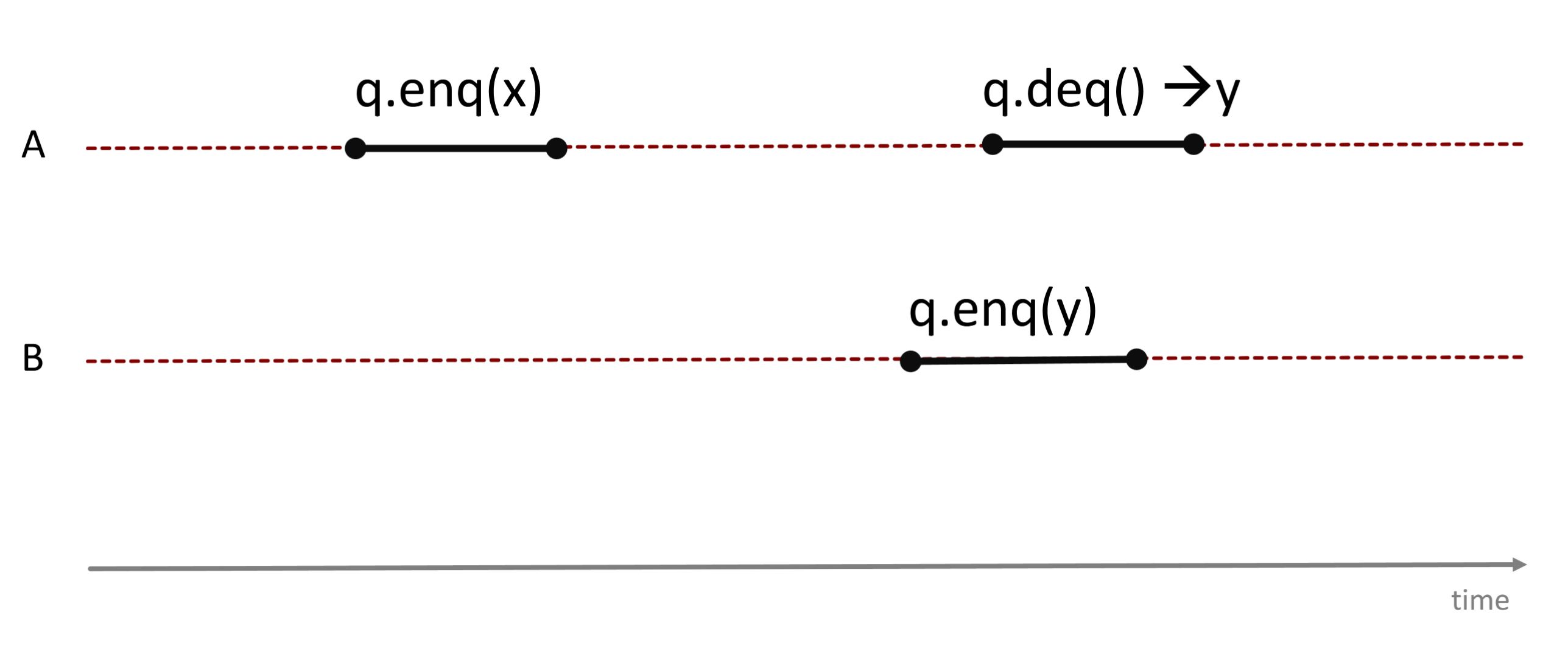
Why is this history sequentially consistent, even though it is not linearizable?
Back
ETH::2._Semester::PProg::12._Linearizability_and_TM::3._Consistency_Models
Why is this history sequentially consistent, even though it is not linearizable?
Not linearizable: since
enq(x) precedes
enq(y) in real time, any order respecting real time must enqueue \(x\) before \(y\), so
deq() would have to return \(x\), not \(y\).
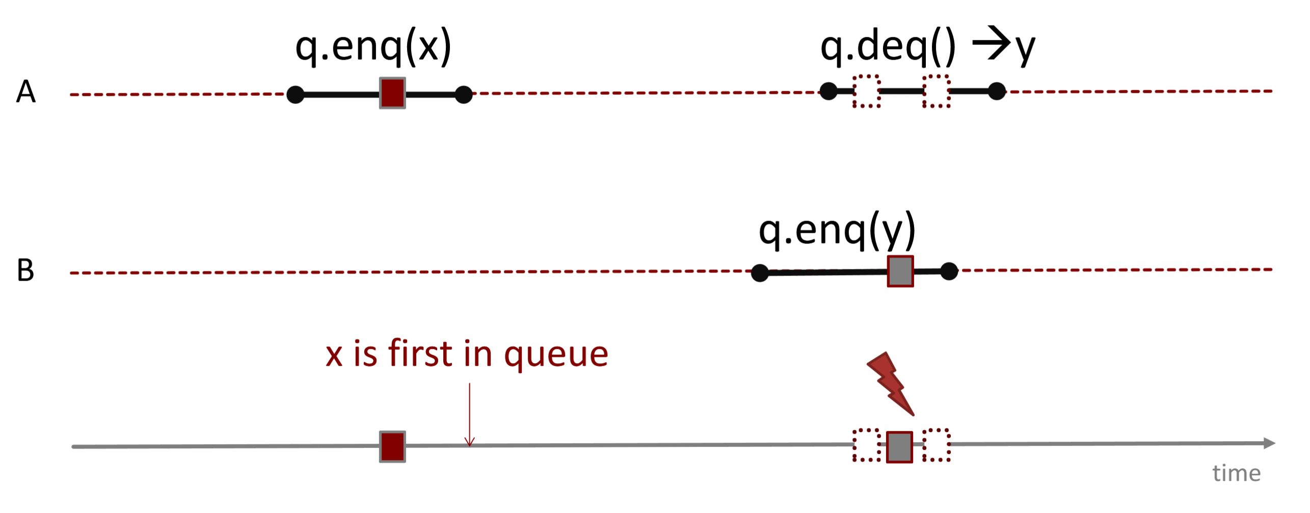
Sequentially consistent: sequential consistency precisely does not require \(\to_G \subseteq \to_S\). You may move B's
enq(y) before A's
enq(x) in \(S\), as long as the program order of each individual thread is preserved. The legal sequential order \(\text{enq}(y),\,\text{enq}(x),\,\text{deq}{\to}y\) is compatible with both thread projections.
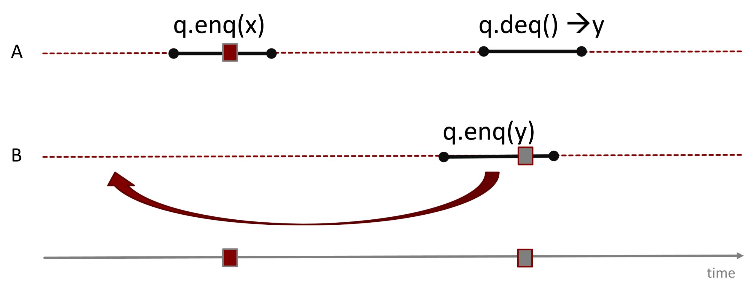
Field-by-field Comparison
| Field |
Before |
After |
| Front |
|
<img src="paste-81faf086155af500a29765383d85cb625837c0f2.jpg"><br><br>Why is this history sequentially consistent, even though it is not linearizable? |
| Back |
|
Not linearizable: since <code>enq(x)</code> precedes <code>enq(y)</code> in real time, any order respecting real time must enqueue \(x\) before \(y\), so <code>deq()</code> would have to return \(x\), not \(y\).<br><img src="paste-488dd281c89faf1fe23190650c429388c6404296.jpg"><br><br>Sequentially consistent: sequential consistency precisely does not require \(\to_G \subseteq \to_S\). You may move B's <code>enq(y)</code> before A's <code>enq(x)</code> in \(S\), as long as the program order of each individual thread is preserved. The legal sequential order \(\text{enq}(y),\,\text{enq}(x),\,\text{deq}{\to}y\) is compatible with both thread projections.<br><img src="paste-dcb95971d76cfc03849747c96e4e6ba6e08b80e9.jpg"> |
Tags:
ETH::2._Semester::PProg::12._Linearizability_and_TM::3._Consistency_Models
Note 146: ETH::2. Semester::PProg
Deck: ETH::2. Semester::PProg
Note Type: Horvath Cloze
GUID: FDyr
added
Previous
Note did not exist
New Note
Front
ETH::2._Semester::PProg::12._Linearizability_and_TM::2._Histories
Two histories \(H\) and \(G\) are equivalent iff they have the same per-thread projections, i.e. \(H\,|\,T = G\,|\,T\) for every thread \(T\).
Back
ETH::2._Semester::PProg::12._Linearizability_and_TM::2._Histories
Two histories \(H\) and \(G\) are equivalent iff they have the same per-thread projections, i.e. \(H\,|\,T = G\,|\,T\) for every thread \(T\).
Equivalence ignores how calls of different threads are interleaved in time; it only cares that each thread sees the same local sequence.
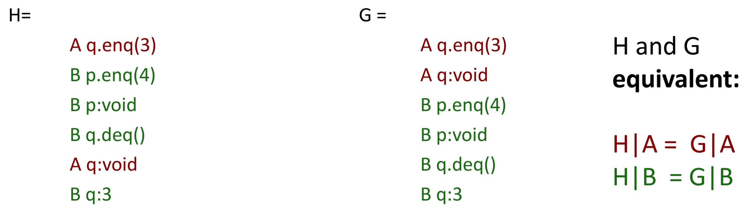
Field-by-field Comparison
| Field |
Before |
After |
| Text |
|
Two histories \(H\) and \(G\) are equivalent iff {{c1::they have the same per-thread projections, i.e. \(H\,|\,T = G\,|\,T\) for every thread \(T\)}}. |
| Extra |
|
Equivalence ignores how calls of different threads are interleaved in time; it only cares that each thread sees the same local sequence.<br><br><img src="paste-7cc292dd73bb623ed6a6212e0b74feaec9b2a5c4.jpg"> |
Tags:
ETH::2._Semester::PProg::12._Linearizability_and_TM::2._Histories
Note 147: ETH::2. Semester::PProg
Deck: ETH::2. Semester::PProg
Note Type: Horvath Cloze
GUID: G,PGY3(|_E
added
Previous
Note did not exist
New Note
Front
ETH::2._Semester::PProg::12._Linearizability_and_TM::1._Linearizability
Important subtlety about linearization points: they can often be named in the code, but they may depend on the execution, not only on the source code.
Example: a deq() on a bounded queue linearizes at different points depending on whether the queue is empty (the call may fail) or non-empty (it does not fail).
Back
ETH::2._Semester::PProg::12._Linearizability_and_TM::1._Linearizability
Important subtlety about linearization points: they can often be named in the code, but they may depend on the execution, not only on the source code.
Example: a deq() on a bounded queue linearizes at different points depending on whether the queue is empty (the call may fail) or non-empty (it does not fail).
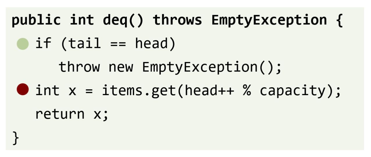
We reason about executions to abstract away from the implementation, but this abstraction has to be mentally undone when actually analysing a program.
Field-by-field Comparison
| Field |
Before |
After |
| Text |
|
Important subtlety about linearization points: they can often be named in the code, but they may depend on {{c1::the execution, not only on the source code}}. <br><br>Example: a <code>deq()</code> on a bounded queue linearizes at {{c2::different points depending on whether the queue is empty (the call may fail) or non-empty (it does not fail)}}. |
| Extra |
|
<img src="paste-d95243cb50fa47ec411c5b3909766ca3ddcd551f.jpg"><br><br>We reason about executions to abstract away from the implementation, but this abstraction has to be mentally undone when actually analysing a program. |
Tags:
ETH::2._Semester::PProg::12._Linearizability_and_TM::1._Linearizability
Note 148: ETH::2. Semester::PProg
Deck: ETH::2. Semester::PProg
Note Type: Horvath Cloze
GUID: IZiu`U~P/,
added
Previous
Note did not exist
New Note
Front
ETH::2._Semester::PProg::12._Linearizability_and_TM::2._Histories
A history \(H\) is well formed if every per-thread projection \(H\,|\,T\) is sequential.
Back
ETH::2._Semester::PProg::12._Linearizability_and_TM::2._Histories
A history \(H\) is well formed if every per-thread projection \(H\,|\,T\) is sequential.
Well-formedness just says each individual thread issues its calls one after another, which any real thread does.
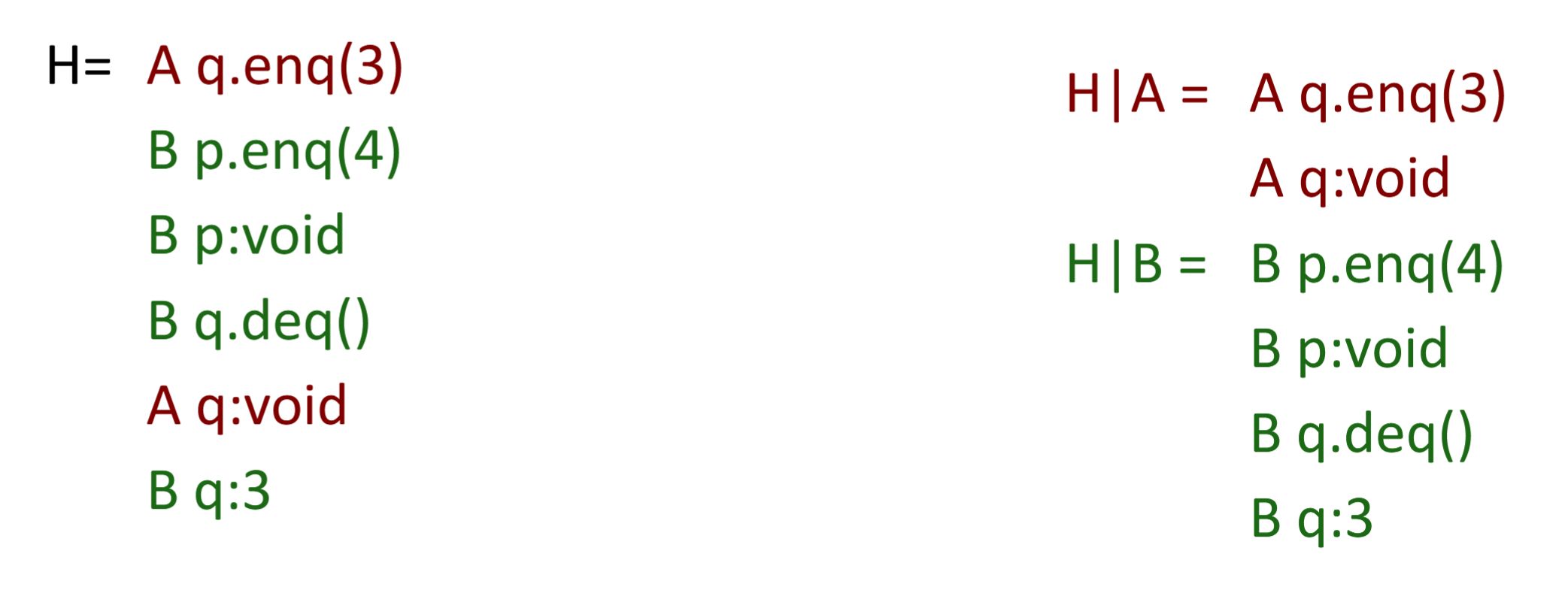
Field-by-field Comparison
| Field |
Before |
After |
| Text |
|
A history \(H\) is well formed if {{c1::every per-thread projection \(H\,|\,T\) is sequential}}. |
| Extra |
|
Well-formedness just says each individual thread issues its calls one after another, which any real thread does.<br><br><img src="paste-00978a8042544bd6fc644d67112b99464812fd1c.jpg"> |
Tags:
ETH::2._Semester::PProg::12._Linearizability_and_TM::2._Histories
Note 149: ETH::2. Semester::PProg
Deck: ETH::2. Semester::PProg
Note Type: Horvath Cloze
GUID: Klwi_:->FQ
added
Previous
Note did not exist
New Note
Front
ETH::2._Semester::PProg::12._Linearizability_and_TM::3._Consistency_Models
Quiescent consistency:
Method calls separated by a period of quiescence (an interval with no pending calls) must take effect in their real-time order; overlapping calls or calls not separated by quiescence may be reordered arbitrarily.
Relative to sequential consistency it is incomparable: neither implies the other.
Back
ETH::2._Semester::PProg::12._Linearizability_and_TM::3._Consistency_Models
Quiescent consistency:
Method calls separated by a period of quiescence (an interval with no pending calls) must take effect in their real-time order; overlapping calls or calls not separated by quiescence may be reordered arbitrarily.
Relative to sequential consistency it is incomparable: neither implies the other.
An example can be sequentially consistent but not quiescently consistent.
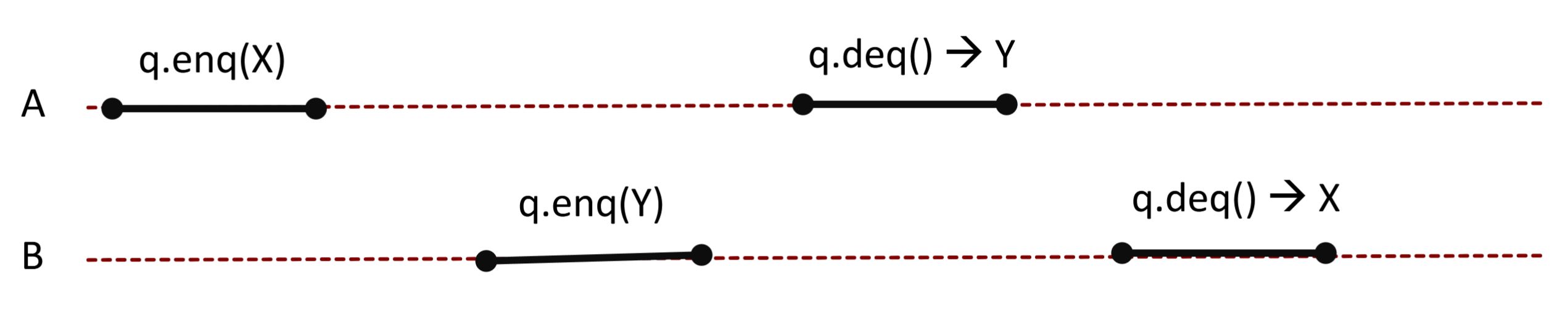
An example can be quiescently consistent but not sequentially consistent (without a quiescent period, even deq and enq may be swapped).
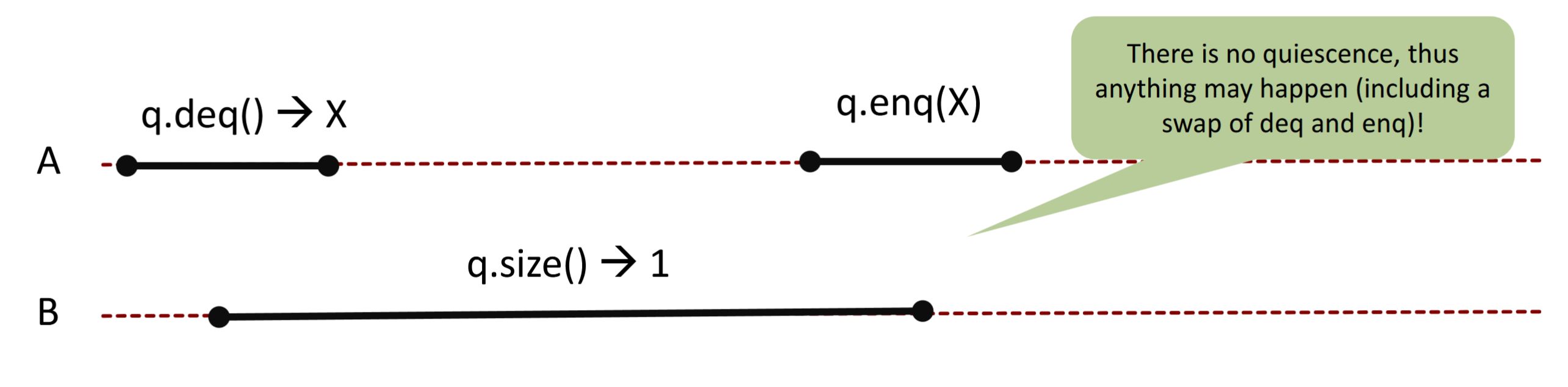
Unlike SC, quiescent consistency does not require preserving the program order within a thread.
Field-by-field Comparison
| Field |
Before |
After |
| Text |
|
Quiescent consistency:<br><br>Method calls separated by a period of quiescence (an interval with no pending calls) must {{c1::take effect in their real-time order}}; overlapping calls or calls not separated by quiescence {{c2::may be reordered arbitrarily}}. <br><br>Relative to sequential consistency it is {{c3::incomparable: neither implies the other}}. |
| Extra |
|
An example can be sequentially consistent but not quiescently consistent.<br><img src="paste-7627f6e046701113c0f292f85640d47d488210b4.jpg"><br><br>An example can be quiescently consistent but not sequentially consistent (without a quiescent period, even deq and enq may be swapped). <br><img src="paste-d64611eeb04a33108264e1a6a67e3ef35685cc6e.jpg"><br><br>Unlike SC, quiescent consistency does not require preserving the program order within a thread. |
Tags:
ETH::2._Semester::PProg::12._Linearizability_and_TM::3._Consistency_Models
Note 150: ETH::2. Semester::PProg
Deck: ETH::2. Semester::PProg
Note Type: Horvath Cloze
GUID: L@08r/Uv,l
added
Previous
Note did not exist
New Note
Front
ETH::2._Semester::PProg::12._Linearizability_and_TM::7._Conflicts_and_Implementation
Implementing TM, two approaches: (1) a big lock around all atomic sections: gives (nearly) all desired properties but is not scalable and is not done in practice. (2) keep track of the operations performed by each transaction (concurrency control): the system guarantees atomicity and isolation.
Back
ETH::2._Semester::PProg::12._Linearizability_and_TM::7._Conflicts_and_Implementation
Implementing TM, two approaches: (1) a big lock around all atomic sections: gives (nearly) all desired properties but is not scalable and is not done in practice. (2) keep track of the operations performed by each transaction (concurrency control): the system guarantees atomicity and isolation.
With the big lock, the missing property is mainly scalability (concurrent transactions cannot run in parallel).
Field-by-field Comparison
| Field |
Before |
After |
| Text |
|
Implementing TM, two approaches: (1) a {{c1::big lock around all atomic sections}}: gives (nearly) all desired properties but is {{c1::not scalable}} and is not done in practice. (2) keep track of the operations performed by each transaction ({{c2::concurrency control}}): the system guarantees {{c2::atomicity and isolation}}. |
| Extra |
|
With the big lock, the missing property is mainly scalability (concurrent transactions cannot run in parallel). |
Tags:
ETH::2._Semester::PProg::12._Linearizability_and_TM::7._Conflicts_and_Implementation
Note 151: ETH::2. Semester::PProg
Deck: ETH::2. Semester::PProg
Note Type: Horvath Cloze
GUID: NVf3SLuVsG
added
Previous
Note did not exist
New Note
Front
ETH::2._Semester::PProg::12._Linearizability_and_TM::2._Histories
Formal definition: a history \(H\) is linearizable if it can be extended to a history \(G\) by
- appending zero or more responses to pending invocations that took effect, and
- discarding zero or more pending invocations that did not take effect,
such that \(G\) is
equivalent to a legal sequential history \(S\) with
\(\to_G \;\subseteq\; \to_S\).
Back
ETH::2._Semester::PProg::12._Linearizability_and_TM::2._Histories
Formal definition: a history \(H\) is linearizable if it can be extended to a history \(G\) by
- appending zero or more responses to pending invocations that took effect, and
- discarding zero or more pending invocations that did not take effect,
such that \(G\) is
equivalent to a legal sequential history \(S\) with
\(\to_G \;\subseteq\; \to_S\).
The condition \(\to_G \subseteq \to_S\) is the crucial one: \(S\) may order overlapping calls freely, but it must respect every real-time precedence already fixed in \(G\). That real-time constraint is what distinguishes linearizability from mere sequential consistency.
Field-by-field Comparison
| Field |
Before |
After |
| Text |
|
Formal definition: a history \(H\) is linearizable if it can be extended to a history \(G\) by <br><ul><li>{{c1::appending zero or more responses to pending invocations that took effect, and}}</li><li>{{c1::discarding zero or more pending invocations that did not take effect}}, </li></ul>such that \(G\) is {{c2::equivalent to a legal sequential history \(S\)}} with {{c3::\(\to_G \;\subseteq\; \to_S\)}}.<br> |
| Extra |
|
The condition \(\to_G \subseteq \to_S\) is the crucial one: \(S\) may order overlapping calls freely, but it must respect every real-time precedence already fixed in \(G\). That real-time constraint is what distinguishes linearizability from mere sequential consistency. |
Tags:
ETH::2._Semester::PProg::12._Linearizability_and_TM::2._Histories
Note 152: ETH::2. Semester::PProg
Deck: ETH::2. Semester::PProg
Note Type: Horvath Cloze
GUID: PS|E1xU1RD
added
Previous
Note did not exist
New Note
Front
ETH::2._Semester::PProg::12._Linearizability_and_TM::1._Linearizability
Linearizability vs. sequential consistency.
Linearizability:
- an operation takes effect instantaneously between invocation and response;
- uses a sequential specification, locality implies composability;
- good for high-level objects (software).
Sequential consistency:
- not composable, but simpler;
- harder for software development;
- good for describing hardware memory models.
Back
ETH::2._Semester::PProg::12._Linearizability_and_TM::1._Linearizability
Linearizability vs. sequential consistency.
Linearizability:
- an operation takes effect instantaneously between invocation and response;
- uses a sequential specification, locality implies composability;
- good for high-level objects (software).
Sequential consistency:
- not composable, but simpler;
- harder for software development;
- good for describing hardware memory models.
Real hardware is even weaker than sequentially consistent (but you can buy SC back at a cost, e.g. memory barriers / volatile). For high-level software, linearizability is the more appropriate concept.
Field-by-field Comparison
| Field |
Before |
After |
| Text |
|
Linearizability vs. sequential consistency. <br><br>Linearizability: <br><ul><li>an operation takes effect {{c1::instantaneously between invocation and response}}; </li><li>uses a sequential specification, locality implies {{c1::composability}}; </li><li>good for {{c1::high-level objects (software)}}. </li></ul>Sequential consistency: <br><ul><li>{{c2::not composable, but simpler}}; </li><li>{{c2::harder for software development}};</li><li>good for {{c2::describing hardware memory models}}.</li></ul> |
| Extra |
|
Real hardware is even weaker than sequentially consistent (but you can buy SC back at a cost, e.g. memory barriers / volatile). For high-level software, linearizability is the more appropriate concept. |
Tags:
ETH::2._Semester::PProg::12._Linearizability_and_TM::1._Linearizability
Note 153: ETH::2. Semester::PProg
Deck: ETH::2. Semester::PProg
Note Type: Horvath Cloze
GUID: R3A[M^O.c5
added
Previous
Note did not exist
New Note
Front
ETH::2._Semester::PProg::12._Linearizability_and_TM::3._Consistency_Models
Properties of sequential consistency:
- operations of a single thread must respect program order;
- the real-time order, by contrast, need not be preserved.
Therefore operations
of the same thread cannot be reordered, but operations
of different threads can be reordered.
It is often used to describe
multiprocessor memory architectures.
Back
ETH::2._Semester::PProg::12._Linearizability_and_TM::3._Consistency_Models
Properties of sequential consistency:
- operations of a single thread must respect program order;
- the real-time order, by contrast, need not be preserved.
Therefore operations
of the same thread cannot be reordered, but operations
of different threads can be reordered.
It is often used to describe
multiprocessor memory architectures.
Mnemonic: program order within a thread stays fixed, everything in between may be swapped. This corresponds exactly to what hardware caches and write buffers allow in practice.
Field-by-field Comparison
| Field |
Before |
After |
| Text |
|
Properties of sequential consistency:<br><ul><li>operations of a single thread must {{c1::respect program order}}; </li><li>the real-time order, by contrast, {{c1::need not be preserved}}.</li></ul>Therefore operations {{c2::of the same thread cannot be reordered}}, but operations {{c2::of different threads can be reordered}}. <br><br>It is often used to describe {{c3::multiprocessor memory architectures}}.<br> |
| Extra |
|
Mnemonic: program order within a thread stays fixed, everything in between may be swapped. This corresponds exactly to what hardware caches and write buffers allow in practice. |
Tags:
ETH::2._Semester::PProg::12._Linearizability_and_TM::3._Consistency_Models
Note 154: ETH::2. Semester::PProg
Deck: ETH::2. Semester::PProg
Note Type: Horvath Classic
GUID: S[({ZB+=[h
added
Previous
Note did not exist
New Note
Front
ETH::2._Semester::PProg::12._Linearizability_and_TM::1._Linearizability
Why is this FIFO-queue execution NOT linearizable?
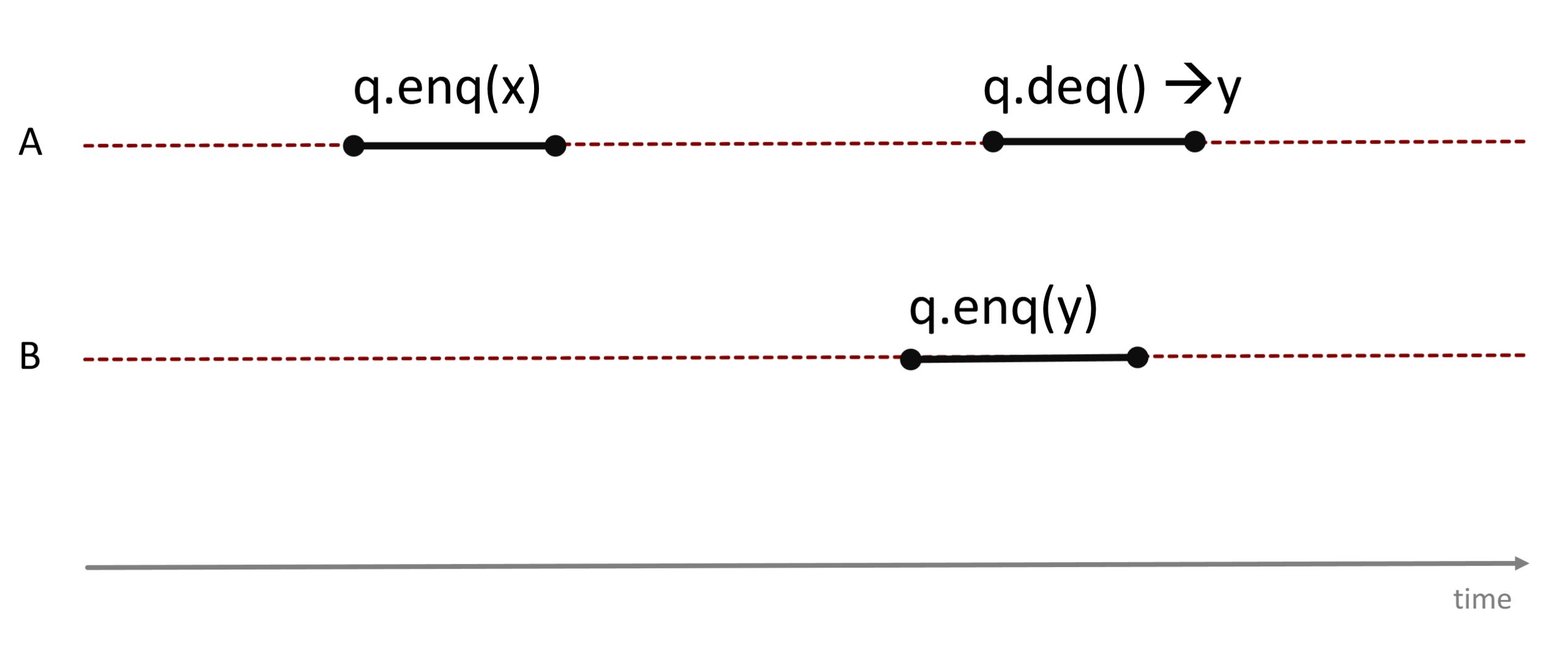
Back
ETH::2._Semester::PProg::12._Linearizability_and_TM::1._Linearizability
Why is this FIFO-queue execution NOT linearizable?
Because
enq(x) precedes
enq(y), every legal sequential order must place \(x\) in the queue before \(y\), so \(x\) is the first element and the first
deq() must return \(x\), not \(y\). No choice of linearization points can reorder two non-overlapping calls, so the FIFO specification is violated and the history is not linearizable.
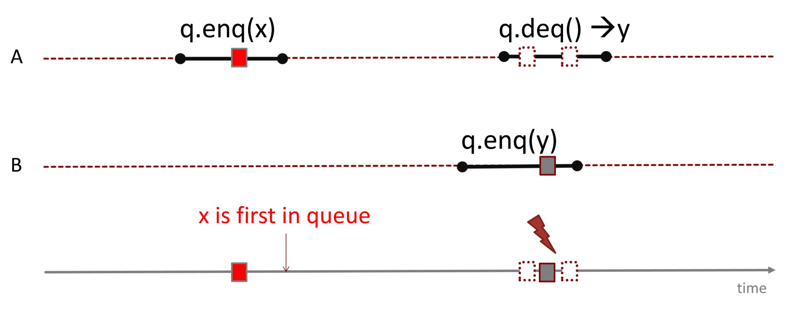
Contrast: when
enq(x) and
enq(y) overlap, either order is admissible and returning \(y\) can be fine.
Field-by-field Comparison
| Field |
Before |
After |
| Front |
|
Why is this FIFO-queue execution NOT linearizable?<br><br><img src="paste-976296ea7860bbace2f5a456cfb1ebf0c76a9469.jpg"> |
| Back |
|
Because <code>enq(x)</code> precedes <code>enq(y)</code>, every legal sequential order must place \(x\) in the queue before \(y\), so \(x\) is the first element and the first <code>deq()</code> must return \(x\), not \(y\). No choice of linearization points can reorder two non-overlapping calls, so the FIFO specification is violated and the history is not linearizable.<br><br><img src="paste-5c5f2f90ad5ab6fd23419c571b974beea73a976d.jpg"><br><br>Contrast: when <code>enq(x)</code> and <code>enq(y)</code> overlap, either order is admissible and returning \(y\) can be fine. |
Tags:
ETH::2._Semester::PProg::12._Linearizability_and_TM::1._Linearizability
Note 155: ETH::2. Semester::PProg
Deck: ETH::2. Semester::PProg
Note Type: Horvath Cloze
GUID: TrD0i9G.}s
added
Previous
Note did not exist
New Note
Front
ETH::2._Semester::PProg::12._Linearizability_and_TM::7._Conflicts_and_Implementation
Hardware TM (HTM): can be fast but has bounded resources and often cannot handle big transactions. The first widely available x86 implementation was Intel's Haswell (RTM), which was largely removed soon after. The Haswell instructions are xbegin (begin transaction), xend (end), xabort (abort).
Back
ETH::2._Semester::PProg::12._Linearizability_and_TM::7._Conflicts_and_Implementation
Hardware TM (HTM): can be fast but has bounded resources and often cannot handle big transactions. The first widely available x86 implementation was Intel's Haswell (RTM), which was largely removed soon after. The Haswell instructions are xbegin (begin transaction), xend (end), xabort (abort).
Other HTM examples: Sun/Oracle Rock (never released), IBM Blue Gene/Q (long retired). Pattern: xbegin L0 / transaction code / xend; on abort, execution jumps to L0.
Field-by-field Comparison
| Field |
Before |
After |
| Text |
|
Hardware TM (HTM): {{c1::can be fast but has bounded resources and often cannot handle big transactions}}. The first widely available x86 implementation was {{c2::Intel's Haswell (RTM)}}, which was largely removed soon after. The Haswell instructions are {{c3::xbegin (begin transaction), xend (end), xabort (abort)}}. |
| Extra |
|
Other HTM examples: Sun/Oracle Rock (never released), IBM Blue Gene/Q (long retired). Pattern: xbegin L0 / transaction code / xend; on abort, execution jumps to L0. |
Tags:
ETH::2._Semester::PProg::12._Linearizability_and_TM::7._Conflicts_and_Implementation
Note 156: ETH::2. Semester::PProg
Deck: ETH::2. Semester::PProg
Note Type: Horvath Cloze
GUID: V*|&Rg$w7`
added
Previous
Note did not exist
New Note
Front
ETH::2._Semester::PProg::11._Lock_Free_Programming::6._Hazard_Pointers
Remarks on the hazard-pointer stack:
- The safe Java version does not actually improve performance over plain allocation plus garbage collection, it merely demonstrates how to solve ABA in principle.
- The hazard pointers live in thread-local storage, and the scheme scales better when that can be replaced by processor-local storage.
Back
ETH::2._Semester::PProg::11._Lock_Free_Programming::6._Hazard_Pointers
Remarks on the hazard-pointer stack:
- The safe Java version does not actually improve performance over plain allocation plus garbage collection, it merely demonstrates how to solve ABA in principle.
- The hazard pointers live in thread-local storage, and the scheme scales better when that can be replaced by processor-local storage.
Höfler's reference to Florian Negele's PhD thesis (ETH Zürich, 2014) on combining lock-free programming with cooperative multitasking.
Field-by-field Comparison
| Field |
Before |
After |
| Text |
|
Remarks on the hazard-pointer stack: <br><ul><li>The safe Java version does {{c1::not actually improve performance over plain allocation plus garbage collection, it merely demonstrates how to solve ABA in principle}}. </li><li>The hazard pointers live in {{c2::thread-local storage}}, and the scheme scales better when that can be replaced by {{c2::processor-local storage}}.</li></ul> |
| Extra |
|
Höfler's reference to Florian Negele's PhD thesis (ETH Zürich, 2014) on combining lock-free programming with cooperative multitasking. |
Tags:
ETH::2._Semester::PProg::11._Lock_Free_Programming::6._Hazard_Pointers
Note 157: ETH::2. Semester::PProg
Deck: ETH::2. Semester::PProg
Note Type: Horvath Cloze
GUID: Zd,;]3fmgt
added
Previous
Note did not exist
New Note
Front
ETH::2._Semester::PProg::12._Linearizability_and_TM::1._Linearizability
A method call is the interval that starts with an invocation event and ends with a response event; between the two it is called pending.
Back
ETH::2._Semester::PProg::12._Linearizability_and_TM::1._Linearizability
A method call is the interval that starts with an invocation event and ends with a response event; between the two it is called pending.
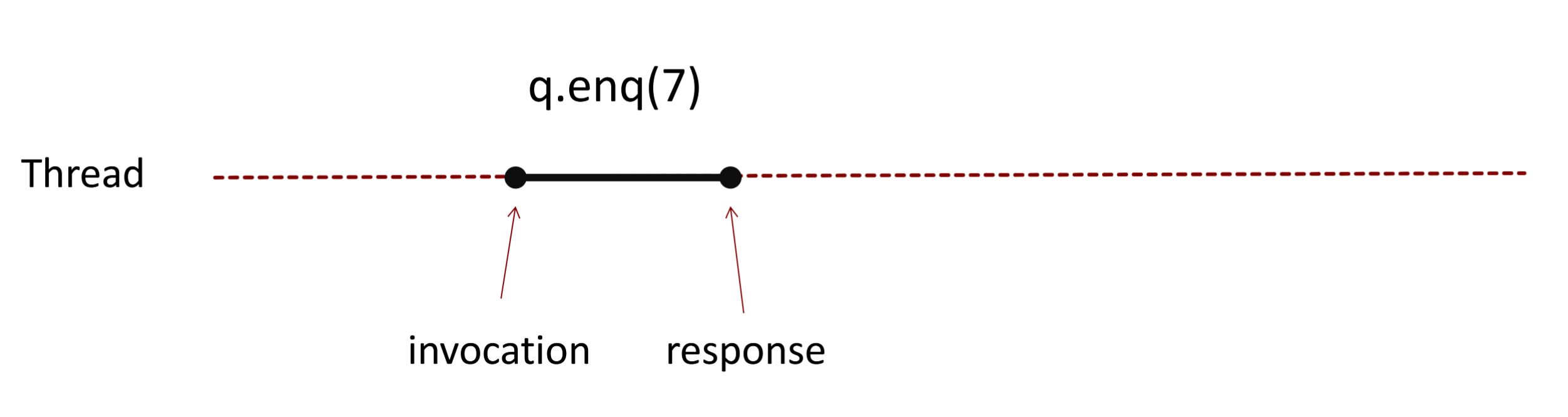
These two events are what the whole linearizability formalism is built on: we reason about the externally visible boundaries of a call, not its source code.
Field-by-field Comparison
| Field |
Before |
After |
| Text |
|
A method call is the interval that starts with an {{c1::invocation}} event and ends with a {{c1::response}} event; between the two it is called {{c2::pending}}. |
| Extra |
|
<img src="paste-55e57c14222f755d7e052b02ca87e8e503e6fd0a.jpg"><br><br>These two events are what the whole linearizability formalism is built on: we reason about the externally visible boundaries of a call, not its source code. |
Tags:
ETH::2._Semester::PProg::12._Linearizability_and_TM::1._Linearizability
Note 158: ETH::2. Semester::PProg
Deck: ETH::2. Semester::PProg
Note Type: Horvath Cloze
GUID: ]]1(@!su9*
added
Previous
Note did not exist
New Note
Front
ETH::2._Semester::PProg::12._Linearizability_and_TM::2._Histories
Terminology on histories:
- An invocation is pending if it has no matching response;
- A subhistory is complete when it contains no pending invocations.
The operation
complete(H) yields
\(H\) with all its pending invocations removed.
Back
ETH::2._Semester::PProg::12._Linearizability_and_TM::2._Histories
Terminology on histories:
- An invocation is pending if it has no matching response;
- A subhistory is complete when it contains no pending invocations.
The operation
complete(H) yields
\(H\) with all its pending invocations removed.
Pending invocations are exactly the calls still in flight at the end of the recorded history.
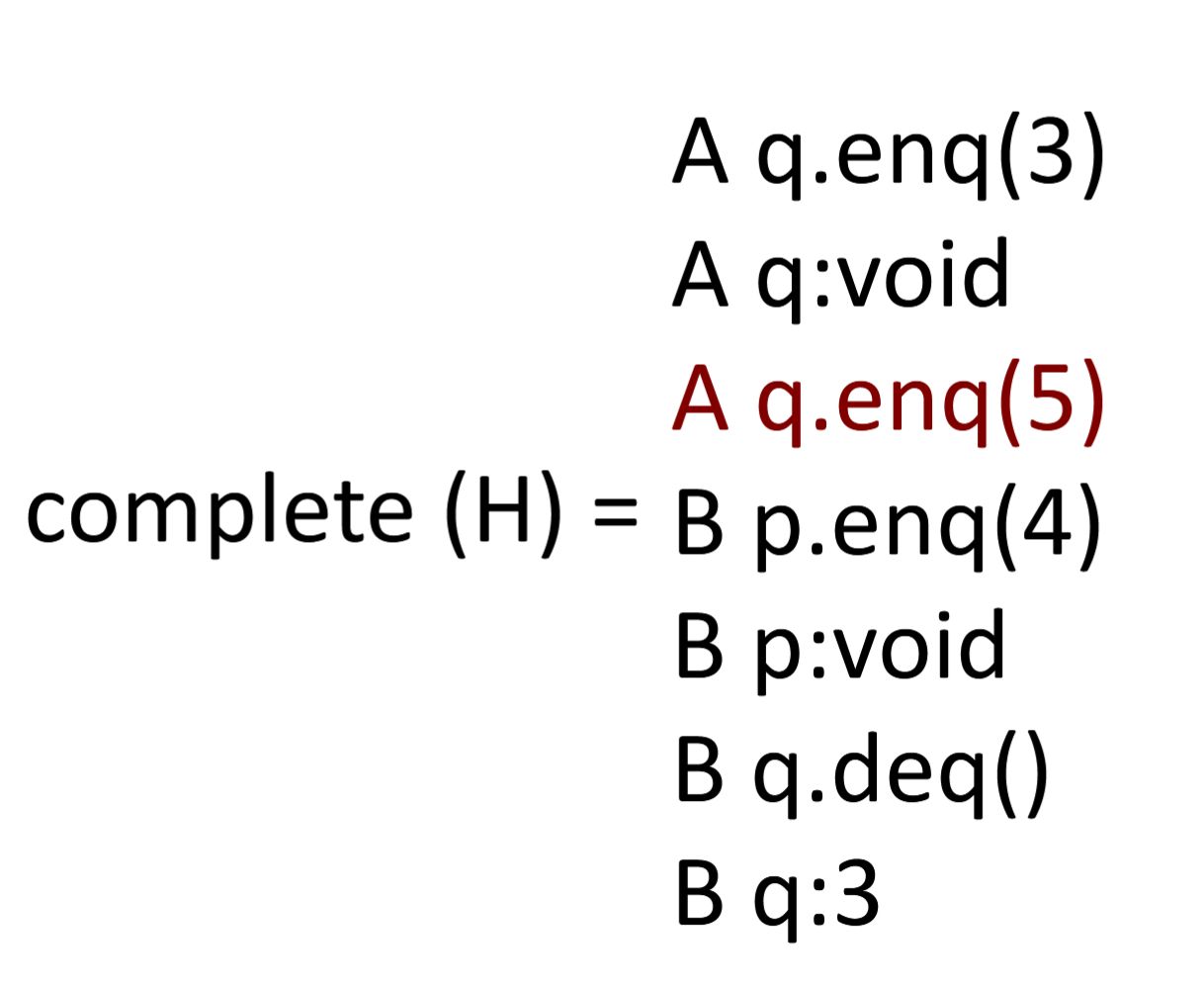
Field-by-field Comparison
| Field |
Before |
After |
| Text |
|
Terminology on histories: <br><ul><li>An invocation is pending if {{c1::it has no matching response}}; </li><li>A subhistory is complete when {{c1::it contains no pending invocations}}. </li></ul>The operation <code>complete(H)</code> yields {{c2::\(H\) with all its pending invocations removed}}.<br> |
| Extra |
|
Pending invocations are exactly the calls still in flight at the end of the recorded history.<br><br><img src="paste-04fbc0f12a7c982c745a408eac7ec417379d5a56.jpg"> |
Tags:
ETH::2._Semester::PProg::12._Linearizability_and_TM::2._Histories
Note 159: ETH::2. Semester::PProg
Deck: ETH::2. Semester::PProg
Note Type: Horvath Classic
GUID: ]]ssC~?k@{
added
Previous
Note did not exist
New Note
Front
ETH::2._Semester::PProg::12._Linearizability_and_TM::4._Consensus
There is no wait-free implementation of a FIFO queue from atomic registers alone. How is this proved (proof idea)?
Back
ETH::2._Semester::PProg::12._Linearizability_and_TM::4._Consensus
There is no wait-free implementation of a FIFO queue from atomic registers alone. How is this proved (proof idea)?
Reduction / contradiction.
- A FIFO queue solves 2-thread consensus (has consensus number \(2\)): the queue is pre-filled with a red and a black ball. Each thread first writes its value into
proposed[i] and then dequeues. Whoever gets the red ball decides its own value; whoever gets the black one reads the winner's value from proposed. This works because the write into the array happens before the dequeue. - Assumption: suppose there were a queue implementation built from atomic registers.
- Substituting it yields a wait-free consensus protocol for 2 threads from atomic registers alone.
- Contradiction: atomic registers have consensus number \(1\). Hence the FIFO queue cannot be implemented from atomic registers.
Field-by-field Comparison
| Field |
Before |
After |
| Front |
|
There is no wait-free implementation of a FIFO queue from atomic registers alone. How is this proved (proof idea)? |
| Back |
|
Reduction / contradiction.<br><ol><li>A FIFO queue solves 2-thread consensus (has consensus number \(2\)): the queue is pre-filled with a red and a black ball. Each thread first writes its value into <code>proposed[i]</code> and then dequeues. Whoever gets the red ball decides its own value; whoever gets the black one reads the winner's value from <code>proposed</code>. This works because the write into the array happens before the dequeue.</li><li>Assumption: suppose there were a queue implementation built from atomic registers.</li><li>Substituting it yields a wait-free consensus protocol for 2 threads from atomic registers alone.</li><li>Contradiction: atomic registers have consensus number \(1\). Hence the FIFO queue cannot be implemented from atomic registers.</li></ol> |
Tags:
ETH::2._Semester::PProg::12._Linearizability_and_TM::4._Consensus
Note 160: ETH::2. Semester::PProg
Deck: ETH::2. Semester::PProg
Note Type: Horvath Cloze
GUID: _Fi_;3y?6+
added
Previous
Note did not exist
New Note
Front
ETH::2._Semester::PProg::12._Linearizability_and_TM::5._Transactional_Memory_Motivation
Core idea of transactional memory:
the burden of synchronisation is moved from the programmer into the system (hardware, software, or both).
The programmer specifies what should be atomic, not how (e.g. via locking) it is made atomic. This is a declarative approach.
Back
ETH::2._Semester::PProg::12._Linearizability_and_TM::5._Transactional_Memory_Motivation
Core idea of transactional memory:
the burden of synchronisation is moved from the programmer into the system (hardware, software, or both).
The programmer specifies what should be atomic, not how (e.g. via locking) it is made atomic. This is a declarative approach.
Motivation from the lecture: programming with locks is too difficult, and lock-free programming is even harder.
Field-by-field Comparison
| Field |
Before |
After |
| Text |
|
Core idea of transactional memory: <br>the burden of synchronisation is moved from the {{c1::programmer}} into the {{c1::system (hardware, software, or both)}}. <br><br>The {{c1::programmer}} specifies {{c2::what}} should be atomic, not {{c2::how (e.g. via locking) it is made atomic}}. This is a {{c3::declarative}} approach. |
| Extra |
|
Motivation from the lecture: programming with locks is too difficult, and lock-free programming is even harder. |
Tags:
ETH::2._Semester::PProg::12._Linearizability_and_TM::5._Transactional_Memory_Motivation
Note 161: ETH::2. Semester::PProg
Deck: ETH::2. Semester::PProg
Note Type: Horvath Cloze
GUID: _Z&YGuT-Pb
added
Previous
Note did not exist
New Note
Front
ETH::2._Semester::PProg::12._Linearizability_and_TM::7._Conflicts_and_Implementation
Nesting semantics for nested transactions (important for composability). Flat nesting: all levels are merged into one transaction, so an inner abort aborts the outer and an inner commit is visible only if the outer commits. Closed nesting (similar, but): an abort of an inner transaction does not abort the outer; an inner commit makes changes visible to the outer transaction but not to other transactions, and only the commit of the outer makes them globally visible.
Back
ETH::2._Semester::PProg::12._Linearizability_and_TM::7._Conflicts_and_Implementation
Nesting semantics for nested transactions (important for composability). Flat nesting: all levels are merged into one transaction, so an inner abort aborts the outer and an inner commit is visible only if the outer commits. Closed nesting (similar, but): an abort of an inner transaction does not abort the outer; an inner commit makes changes visible to the outer transaction but not to other transactions, and only the commit of the outer makes them globally visible.
Another approach: open nesting. Nested transactions are the prerequisite for atomic blocks to be composable.
Field-by-field Comparison
| Field |
Before |
After |
| Text |
|
Nesting semantics for nested transactions (important for composability). Flat nesting: all levels are merged into one transaction, so {{c1::an inner abort aborts the outer}} and an inner commit is {{c1::visible only if the outer commits}}. Closed nesting (similar, but): {{c2::an abort of an inner transaction does not abort the outer}}; an inner commit makes changes {{c2::visible to the outer transaction but not to other transactions}}, and only the commit of the outer makes them {{c2::globally visible}}. |
| Extra |
|
Another approach: open nesting. Nested transactions are the prerequisite for atomic blocks to be composable. |
Tags:
ETH::2._Semester::PProg::12._Linearizability_and_TM::7._Conflicts_and_Implementation
Note 162: ETH::2. Semester::PProg
Deck: ETH::2. Semester::PProg
Note Type: Horvath Cloze
GUID: a`iuMPW&2?
added
Previous
Note did not exist
New Note
Front
ETH::2._Semester::PProg::12._Linearizability_and_TM::5._Transactional_Memory_Motivation
Four problems of locks (motivation for transactional memory):
- Deadlocks (threads take shared or dependent locks in different orders);
- Convoying (a thread holding a resource is descheduled while other threads queue up waiting for it);
- Priority inversion (a low-priority thread holds a resource a high-priority thread is waiting on);
- the association of locks and data exists only by convention (documented in comments at best, not enforced by the program).
Back
ETH::2._Semester::PProg::12._Linearizability_and_TM::5._Transactional_Memory_Motivation
Four problems of locks (motivation for transactional memory):
- Deadlocks (threads take shared or dependent locks in different orders);
- Convoying (a thread holding a resource is descheduled while other threads queue up waiting for it);
- Priority inversion (a low-priority thread holds a resource a high-priority thread is waiting on);
- the association of locks and data exists only by convention (documented in comments at best, not enforced by the program).
These are properties of the lock mechanism itself, not of a specific bug. TM aims to remove them by moving synchronisation from the programmer into the system.
Field-by-field Comparison
| Field |
Before |
After |
| Text |
|
Four problems of locks (motivation for transactional memory): <br><ol><li>{{c1::Deadlocks (threads take shared or dependent locks in different orders)}}; </li><li>{{c2::Convoying (a thread holding a resource is descheduled while other threads queue up waiting for it)}}; </li><li>{{c3::Priority inversion (a low-priority thread holds a resource a high-priority thread is waiting on)}}; </li><li>{{c4::the association of locks and data exists only by convention (documented in comments at best, not enforced by the program)}}.</li></ol> |
| Extra |
|
These are properties of the lock mechanism itself, not of a specific bug. TM aims to remove them by moving synchronisation from the programmer into the system. |
Tags:
ETH::2._Semester::PProg::12._Linearizability_and_TM::5._Transactional_Memory_Motivation
Note 163: ETH::2. Semester::PProg
Deck: ETH::2. Semester::PProg
Note Type: Horvath Cloze
GUID: arwH:P-JN$
added
Previous
Note did not exist
New Note
Front
ETH::2._Semester::PProg::11._Lock_Free_Programming::5._ABA_Problem
Pointer tagging exploits that aligned addresses leave some low bits unused:
a pointer aligned modulo \(32\) frees up \(5\) bits for a tag (in addition to the unused high address bits).
Each time a pointer is stored in the data structure, the tag is incremented by one, and the data structure is accessed via the masked address \(x - (x \bmod 32)\).
Back
ETH::2._Semester::PProg::11._Lock_Free_Programming::5._ABA_Problem
Pointer tagging exploits that aligned addresses leave some low bits unused:
a pointer aligned modulo \(32\) frees up \(5\) bits for a tag (in addition to the unused high address bits).
Each time a pointer is stored in the data structure, the tag is incremented by one, and the data structure is accessed via the masked address \(x - (x \bmod 32)\).

With 5 tag bits there are 32 distinct versions of each pointer, so a recycled pointer almost always carries a different tag and the stale CAS fails. It only delays ABA (the tag eventually wraps around), it does not eliminate it.
Field-by-field Comparison
| Field |
Before |
After |
| Text |
|
Pointer tagging exploits that aligned addresses leave some low bits unused: <br>a pointer aligned modulo \(32\) frees up {{c1::\(5\)}} bits for a tag (in addition to the unused high address bits). <br><br>Each time a pointer is stored in the data structure, the tag is {{c2::incremented by one}}, and the data structure is accessed via the masked address {{c3::\(x - (x \bmod 32)\)}}. |
| Extra |
|
<img src="paste-bcc75c9dc878767b60653d4a5b94a79d93155f78.jpg"><br><br>With 5 tag bits there are 32 distinct versions of each pointer, so a recycled pointer almost always carries a different tag and the stale CAS fails. It only delays ABA (the tag eventually wraps around), it does not eliminate it. |
Tags:
ETH::2._Semester::PProg::11._Lock_Free_Programming::5._ABA_Problem
Note 164: ETH::2. Semester::PProg
Deck: ETH::2. Semester::PProg
Note Type: Horvath Cloze
GUID: faU(b}g;cm
added
Previous
Note did not exist
New Note
Front
ETH::2._Semester::PProg::12._Linearizability_and_TM::5._Transactional_Memory_Motivation
Analogy for the importance of consensus (squaring the circle):
Just as there is an algebraic proof that squaring the circle with compass and straightedge is impossible, there is a proof that certain wait-free algorithms cannot be constructed from atomic registers.
Lesson: do not try anyway.
Back
ETH::2._Semester::PProg::12._Linearizability_and_TM::5._Transactional_Memory_Motivation
Analogy for the importance of consensus (squaring the circle):
Just as there is an algebraic proof that squaring the circle with compass and straightedge is impossible, there is a proof that certain wait-free algorithms cannot be constructed from atomic registers.
Lesson: do not try anyway.
The consensus hierarchy is therefore not a mere detail but a hard impossibility bound: it tells you in advance which synchronisation goals are achievable with which primitives.
Field-by-field Comparison
| Field |
Before |
After |
| Text |
|
Analogy for the importance of consensus (squaring the circle): <br><br>Just as there is an algebraic proof that squaring the circle with compass and straightedge is {{c1::impossible}}, there is a proof that certain wait-free algorithms {{c1::cannot be constructed from atomic registers}}. <br><br>Lesson: do not try anyway. |
| Extra |
|
The consensus hierarchy is therefore not a mere detail but a hard impossibility bound: it tells you in advance which synchronisation goals are achievable with which primitives. |
Tags:
ETH::2._Semester::PProg::12._Linearizability_and_TM::5._Transactional_Memory_Motivation
Note 165: ETH::2. Semester::PProg
Deck: ETH::2. Semester::PProg
Note Type: Horvath Cloze
GUID: iN)YBu=)cR
added
Previous
Note did not exist
New Note
Front
ETH::2._Semester::PProg::12._Linearizability_and_TM::3._Consistency_Models
A history \(H\) is sequentially consistent if it can be extended to a history \(G\) (appending responses to effective pending invocations, discarding ineffective ones) such that \(G\) is equivalent to a legal sequential history \(S\).
Unlike linearizability, \(\to_G \;\subseteq\; \to_S\) is not required here, i.e. no ordering across threads is demanded.
Back
ETH::2._Semester::PProg::12._Linearizability_and_TM::3._Consistency_Models
A history \(H\) is sequentially consistent if it can be extended to a history \(G\) (appending responses to effective pending invocations, discarding ineffective ones) such that \(G\) is equivalent to a legal sequential history \(S\).
Unlike linearizability, \(\to_G \;\subseteq\; \to_S\) is not required here, i.e. no ordering across threads is demanded.
Exactly this missing real-time constraint makes sequential consistency weaker than linearizability: every linearizable history is sequentially consistent, but not vice versa.
Field-by-field Comparison
| Field |
Before |
After |
| Text |
|
A history \(H\) is sequentially consistent if it can be extended to a history \(G\) (appending responses to effective pending invocations, discarding ineffective ones) such that \(G\) is {{c1::equivalent to a legal sequential history \(S\)}}. <br><br>Unlike linearizability, {{c2::\(\to_G \;\subseteq\; \to_S\) is not required}} here, i.e. {{c2::no ordering across threads is demanded}}. |
| Extra |
|
Exactly this missing real-time constraint makes sequential consistency weaker than linearizability: every linearizable history is sequentially consistent, but not vice versa. |
Tags:
ETH::2._Semester::PProg::12._Linearizability_and_TM::3._Consistency_Models
Note 166: ETH::2. Semester::PProg
Deck: ETH::2. Semester::PProg
Note Type: Horvath Cloze
GUID: j&9s{EU~Gy
added
Previous
Note did not exist
New Note
Front
ETH::2._Semester::PProg::12._Linearizability_and_TM::4._Consensus
Compare-And-Swap has consensus number \(\infty\).
Back
ETH::2._Semester::PProg::12._Linearizability_and_TM::4._Consensus
Compare-And-Swap has consensus number \(\infty\).
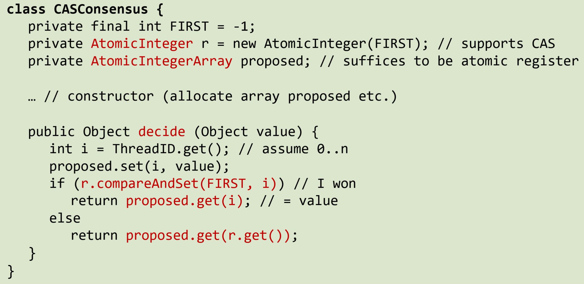
Writing into
proposed before the CAS guarantees that the winner's value is visible to all.
Field-by-field Comparison
| Field |
Before |
After |
| Text |
|
Compare-And-Swap has consensus number {{c1::\(\infty\)}}. |
| Extra |
|
<img src="paste-dbedf400b5a9d74837c9463e17153cd3712481bd.jpg"><br><br>Writing into <code>proposed</code><span style="font-family: "Liberation Sans";"> before the CAS guarantees that the winner's value is visible to all.</span><br> |
Tags:
ETH::2._Semester::PProg::12._Linearizability_and_TM::4._Consensus
Note 167: ETH::2. Semester::PProg
Deck: ETH::2. Semester::PProg
Note Type: Horvath Cloze
GUID: j&UK790c$]
added
Previous
Note did not exist
New Note
Front
ETH::2._Semester::PProg::12._Linearizability_and_TM::7._Conflicts_and_Implementation
Conflict example (initially a = 0): TXA reads x = a, TXB writes a = 10 and then commits. Question: may TXA be placed after TXB in the serialization order if TXA still read a == 0? Answer: no. In the serial order TXB then TXA, TXA would have to read a == 10; executions that read a == 0 are invalid.
Back
ETH::2._Semester::PProg::12._Linearizability_and_TM::7._Conflicts_and_Implementation
Conflict example (initially a = 0): TXA reads x = a, TXB writes a = 10 and then commits. Question: may TXA be placed after TXB in the serialization order if TXA still read a == 0? Answer: no. In the serial order TXB then TXA, TXA would have to read a == 10; executions that read a == 0 are invalid.
A transaction's local writes become visible to others only after commit. Such a read-write conflict is detected and handled by the concurrency-control mechanism.
Field-by-field Comparison
| Field |
Before |
After |
| Text |
|
Conflict example (initially a = 0): TXA reads x = a, TXB writes a = 10 and then commits. Question: may TXA be placed after TXB in the serialization order if TXA still read a == 0? Answer: {{c1::no}}. In the serial order TXB then TXA, TXA would have to {{c2::read a == 10}}; executions that read a == 0 are {{c3::invalid}}. |
| Extra |
|
A transaction's local writes become visible to others only after commit. Such a read-write conflict is detected and handled by the concurrency-control mechanism. |
Tags:
ETH::2._Semester::PProg::12._Linearizability_and_TM::7._Conflicts_and_Implementation
Note 168: ETH::2. Semester::PProg
Deck: ETH::2. Semester::PProg
Note Type: Horvath Cloze
GUID: l-sY%5?jpc
added
Previous
Note did not exist
New Note
Front
ETH::2._Semester::PProg::12._Linearizability_and_TM::6._Transactional_Memory_Semantics
Solution matching the programmer's intent: an atomic block
atomic {
    a.withdraw(amount);
    b.deposit(amount);
}
This is the core idea of transactional memory. The wish to be atomic is
also behind locks: the difference lies in the
execution.
Back
ETH::2._Semester::PProg::12._Linearizability_and_TM::6._Transactional_Memory_Semantics
Solution matching the programmer's intent: an atomic block
atomic {
    a.withdraw(amount);
    b.deposit(amount);
}
This is the core idea of transactional memory. The wish to be atomic is
also behind locks: the difference lies in the
execution.
Locks and TM express the same wish (execute atomically), but TM realises it optimistically without mutual exclusion instead of pessimistically via mutual exclusion.
Field-by-field Comparison
| Field |
Before |
After |
| Text |
|
Solution matching the programmer's intent: an atomic block <pre>atomic {
a.withdraw(amount);
b.deposit(amount);
}</pre> This is the core idea of transactional memory. The wish to be atomic is {{c1::also behind locks}}: the difference lies in the {{c2::execution}}. |
| Extra |
|
Locks and TM express the same wish (execute atomically), but TM realises it optimistically without mutual exclusion instead of pessimistically via mutual exclusion. |
Tags:
ETH::2._Semester::PProg::12._Linearizability_and_TM::6._Transactional_Memory_Semantics
Note 169: ETH::2. Semester::PProg
Deck: ETH::2. Semester::PProg
Note Type: Horvath Cloze
GUID: m)lBDJ?7es
added
Previous
Note did not exist
New Note
Front
ETH::2._Semester::PProg::11._Lock_Free_Programming::6._Hazard_Pointers
Two helper methods backing the global hazard array
AtomicReferenceArray<Node> hazarduous (sized
nThreads):
setHazardous(node) writes into the calling thread's own slot: hazarduous.set(id, node);isHazardous(node) scans every slot and returns true if any slot equals node.
Back
ETH::2._Semester::PProg::11._Lock_Free_Programming::6._Hazard_Pointers
Two helper methods backing the global hazard array
AtomicReferenceArray<Node> hazarduous (sized
nThreads):
setHazardous(node) writes into the calling thread's own slot: hazarduous.set(id, node);isHazardous(node) scans every slot and returns true if any slot equals node.
set touches only the current thread's index id; the check is a full linear scan over all nThreads slots, hence O(nThreads) per reuse.
Field-by-field Comparison
| Field |
Before |
After |
| Text |
|
Two helper methods backing the global hazard array <code>AtomicReferenceArray<Node> hazarduous</code> (sized <code>nThreads</code>): <ul><li><code>setHazardous(node)</code> {{c1::writes into the calling thread's own slot: <code>hazarduous.set(id, node)</code>}};</li><li><code>isHazardous(node)</code> {{c2::scans every slot and returns true if any slot equals <code>node</code>}}.</li></ul> |
| Extra |
|
<code>set</code> touches only the current thread's index <code>id</code>; the check is a full linear scan over all <code>nThreads</code> slots, hence O(nThreads) per reuse. |
Tags:
ETH::2._Semester::PProg::11._Lock_Free_Programming::6._Hazard_Pointers
Note 170: ETH::2. Semester::PProg
Deck: ETH::2. Semester::PProg
Note Type: Horvath Cloze
GUID: oV,4c+Xtxb
added
Previous
Note did not exist
New Note
Front
ETH::2._Semester::PProg::11._Lock_Free_Programming::6._Hazard_Pointers
Hazard-pointer
pop protects
head before using it.
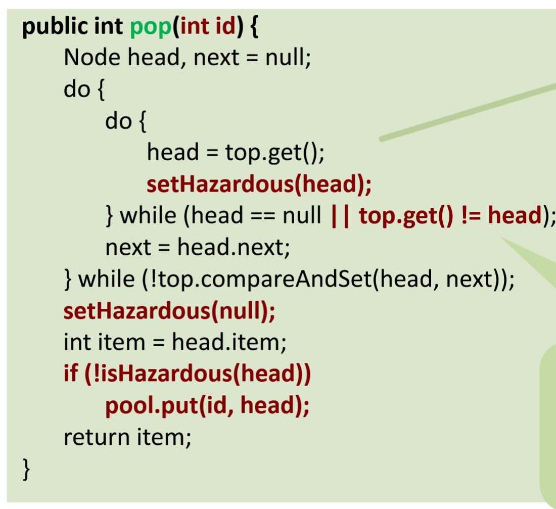
After reading
head = top.get() and calling
setHazardous(head), the inner loop re-checks the condition
head == null || top.get() != head and retries if it holds.
This re-read is essential because it ensures that
no other thread is already past its CAS without having seen our hazard pointer (i.e. top still equals the node we just flagged).
Back
ETH::2._Semester::PProg::11._Lock_Free_Programming::6._Hazard_Pointers
Hazard-pointer
pop protects
head before using it.
After reading
head = top.get() and calling
setHazardous(head), the inner loop re-checks the condition
head == null || top.get() != head and retries if it holds.
This re-read is essential because it ensures that
no other thread is already past its CAS without having seen our hazard pointer (i.e. top still equals the node we just flagged).
Order matters: publish the hazard pointer first, then validate that top is unchanged. Without the re-validation a reclaimer could have slipped between the read and the setHazardous.
Field-by-field Comparison
| Field |
Before |
After |
| Text |
|
Hazard-pointer <code>pop</code> protects <code>head</code> before using it.<br><br><img src="paste-78e79af765fdd52c9fafd13c9b938bda514da0a1.jpg"><br><br> After reading <code>head = top.get()</code> and calling <code>setHazardous(head)</code>, the inner loop re-checks the condition <code>head == null || top.get() != head</code> and retries if it holds. <br><br>This re-read is essential because it ensures that {{c1::no other thread is already past its CAS without having seen our hazard pointer (i.e. <code>top</code> still equals the node we just flagged)}}. |
| Extra |
|
Order matters: publish the hazard pointer first, <em>then</em> validate that <code>top</code> is unchanged. Without the re-validation a reclaimer could have slipped between the read and the <code>setHazardous</code>. |
Tags:
ETH::2._Semester::PProg::11._Lock_Free_Programming::6._Hazard_Pointers
Note 171: ETH::2. Semester::PProg
Deck: ETH::2. Semester::PProg
Note Type: Horvath Cloze
GUID: p
added
Previous
Note did not exist
New Note
Front
ETH::2._Semester::PProg::12._Linearizability_and_TM::2._Histories
Precedence of method calls in a history.
A method call precedes another iff its response event occurs before the other call's invocation event; if neither precedes the other, the two calls overlap (are concurrent).
Written \(m_0 \to_H m_1\), this relation is a partial order on \(H\), which becomes total exactly when \(H\) is sequential.
Back
ETH::2._Semester::PProg::12._Linearizability_and_TM::2._Histories
Precedence of method calls in a history.
A method call precedes another iff its response event occurs before the other call's invocation event; if neither precedes the other, the two calls overlap (are concurrent).
Written \(m_0 \to_H m_1\), this relation is a partial order on \(H\), which becomes total exactly when \(H\) is sequential.
This is the method-call-level precedence (built on whole calls), distinct from the event-level precedence used in the lock proofs.
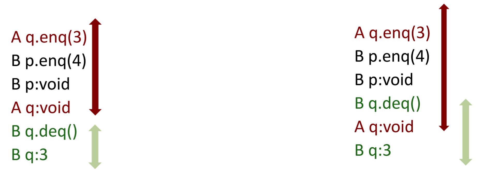
Field-by-field Comparison
| Field |
Before |
After |
| Text |
|
Precedence of method calls in a history.<br>A method call {{c1::precedes another iff its response event occurs before the other call's invocation event}}; if neither precedes the other, the two calls {{c2::overlap (are concurrent)}}. <br><br>Written \(m_0 \to_H m_1\), this relation is {{c3::a partial order on \(H\), which becomes total exactly when \(H\) is sequential}}. |
| Extra |
|
This is the method-call-level precedence (built on whole calls), distinct from the event-level precedence used in the lock proofs.<br><br><img src="paste-a6c108098cbecfebb6ea2cbd231a0686c1330b4e.jpg"> |
Tags:
ETH::2._Semester::PProg::12._Linearizability_and_TM::2._Histories
Note 172: ETH::2. Semester::PProg
Deck: ETH::2. Semester::PProg
Note Type: Horvath Cloze
GUID: pAi0T@*1-#
added
Previous
Note did not exist
New Note
Front
ETH::2._Semester::PProg::11._Lock_Free_Programming::5._ABA_Problem
Four ways to defend against the ABA problem on CAS:
- DCAS (double compare-and-swap): not available on most platforms;
- garbage collection: a node is not freed/reused while a pointer to it still exists, but it is far too slow for the inner loop of a runtime kernel;
- pointer tagging: does not cure the problem, only makes it much less likely (delays it);
- hazard pointers (and transactional memory).
Back
ETH::2._Semester::PProg::11._Lock_Free_Programming::5._ABA_Problem
Four ways to defend against the ABA problem on CAS:
- DCAS (double compare-and-swap): not available on most platforms;
- garbage collection: a node is not freed/reused while a pointer to it still exists, but it is far too slow for the inner loop of a runtime kernel;
- pointer tagging: does not cure the problem, only makes it much less likely (delays it);
- hazard pointers (and transactional memory).
GC is itself the reason a lock-free GC cannot rely on GC to dodge ABA. Tagging can be practical but must be used very carefully.
Field-by-field Comparison
| Field |
Before |
After |
| Text |
|
Four ways to defend against the ABA problem on CAS: <ol><li>{{c1::DCAS (double compare-and-swap): not available on most platforms}};</li><li>{{c2::garbage collection: a node is not freed/reused while a pointer to it still exists, but it is far too slow for the inner loop of a runtime kernel}};</li><li>{{c3::pointer tagging: does not cure the problem, only makes it much less likely (delays it)}};</li><li>{{c4::hazard pointers (and transactional memory)}}.</li></ol> |
| Extra |
|
GC is itself the reason a lock-free GC cannot rely on GC to dodge ABA. Tagging can be practical but must be used very carefully. |
Tags:
ETH::2._Semester::PProg::11._Lock_Free_Programming::5._ABA_Problem
Note 173: ETH::2. Semester::PProg
Deck: ETH::2. Semester::PProg
Note Type: Horvath Cloze
GUID: pu0IY<}%/>
added
Previous
Note did not exist
New Note
Front
ETH::2._Semester::PProg::12._Linearizability_and_TM::2._Histories
A history is sequential if method calls of different threads do not interleave (each invocation is immediately followed by its matching response).
The one exception allowed is a single final pending invocation.
Back
ETH::2._Semester::PProg::12._Linearizability_and_TM::2._Histories
A history is sequential if method calls of different threads do not interleave (each invocation is immediately followed by its matching response).
The one exception allowed is a single final pending invocation.
Sequential here is about non-interleaving of events, independent of how many threads appear.
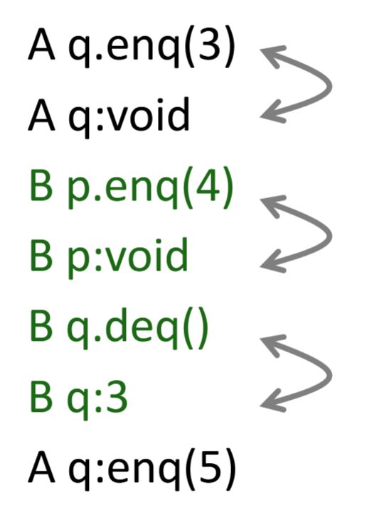
Field-by-field Comparison
| Field |
Before |
After |
| Text |
|
A history is sequential if {{c1::method calls of different threads do not interleave (each invocation is immediately followed by its matching response)}}. <br><br>The one exception allowed is {{c2::a single final pending invocation}}. |
| Extra |
|
Sequential here is about non-interleaving of events, independent of how many threads appear.<br><br><img src="paste-f0e68ca249ee8f5e5a08eb58f798a094dfb46d1c.jpg"> |
Tags:
ETH::2._Semester::PProg::12._Linearizability_and_TM::2._Histories
Note 174: ETH::2. Semester::PProg
Deck: ETH::2. Semester::PProg
Note Type: Horvath Cloze
GUID: q7[aG2i*rq
added
Previous
Note did not exist
New Note
Front
ETH::2._Semester::PProg::11._Lock_Free_Programming::6._Hazard_Pointers
Lessons learned about lock-free programming versus lock-based:
- Atomic update of several pointers/values at once is impossible, which forces new techniques such as threads that help each other to guarantee global progress.
- The ABA problem often disappears under a garbage collector, but beware: ABA on plain values (not pointers) is NOT prevented by GC.
Back
ETH::2._Semester::PProg::11._Lock_Free_Programming::6._Hazard_Pointers
Lessons learned about lock-free programming versus lock-based:
- Atomic update of several pointers/values at once is impossible, which forces new techniques such as threads that help each other to guarantee global progress.
- The ABA problem often disappears under a garbage collector, but beware: ABA on plain values (not pointers) is NOT prevented by GC.
GC keeps a referenced node alive (preventing pointer reuse), but it has nothing to say about a counter or flag that legitimately goes A -> B -> A.
Field-by-field Comparison
| Field |
Before |
After |
| Text |
|
Lessons learned about lock-free programming versus lock-based: <br><ol><li>Atomic update of several pointers/values at once is impossible, which forces new techniques such as {{c1::threads that help each other to guarantee global progress}}. </li><li>The ABA problem often disappears under a garbage collector, but beware: {{c2::ABA on plain values (not pointers) is NOT prevented by GC}}.</li></ol> |
| Extra |
|
GC keeps a referenced node alive (preventing pointer reuse), but it has nothing to say about a counter or flag that legitimately goes A -> B -> A. |
Tags:
ETH::2._Semester::PProg::11._Lock_Free_Programming::6._Hazard_Pointers
Note 175: ETH::2. Semester::PProg
Deck: ETH::2. Semester::PProg
Note Type: Horvath Cloze
GUID: r~,bQfb)e.
added
Previous
Note did not exist
New Note
Front
ETH::2._Semester::PProg::11._Lock_Free_Programming::6._Hazard_Pointers
After the successful CAS in the hazard-pointer pop, the thread calls setHazardous(null) to clear its slot, and only returns the node to the pool if !isHazardous(head), i.e. no other thread still has it flagged.
Back
ETH::2._Semester::PProg::11._Lock_Free_Programming::6._Hazard_Pointers
After the successful CAS in the hazard-pointer pop, the thread calls setHazardous(null) to clear its slot, and only returns the node to the pool if !isHazardous(head), i.e. no other thread still has it flagged.
If the node is still hazardous it is simply not pooled; some thread holding it as hazardous is responsible. push is unchanged from the plain lock-free stack.
Field-by-field Comparison
| Field |
Before |
After |
| Text |
|
After the successful CAS in the hazard-pointer <code>pop</code>, the thread calls {{c1::<code>setHazardous(null)</code>}} to clear its slot, and only returns the node to the pool if {{c2::<code>!isHazardous(head)</code>, i.e. no other thread still has it flagged}}. |
| Extra |
|
If the node is still hazardous it is simply not pooled; some thread holding it as hazardous is responsible. <code>push</code> is unchanged from the plain lock-free stack. |
Tags:
ETH::2._Semester::PProg::11._Lock_Free_Programming::6._Hazard_Pointers
Note 176: ETH::2. Semester::PProg
Deck: ETH::2. Semester::PProg
Note Type: Horvath Cloze
GUID: t]xjImD9{]
added
Previous
Note did not exist
New Note
Front
ETH::2._Semester::PProg::12._Linearizability_and_TM::5._Transactional_Memory_Motivation
Locks are not composable:
To combine \(n\) thread-safe operations you need internal details about their locking.
Moreover, ensuring the correct lock ordering is ad-hoc and not part of the program (documented in comments at best). This is especially problematic for programming in the large.
Back
ETH::2._Semester::PProg::12._Linearizability_and_TM::5._Transactional_Memory_Motivation
Locks are not composable:
To combine \(n\) thread-safe operations you need internal details about their locking.
Moreover, ensuring the correct lock ordering is ad-hoc and not part of the program (documented in comments at best). This is especially problematic for programming in the large.
Composability is the central advantage of TM over locks: atomic blocks can be nested without knowing the internals of the inner operations.
Field-by-field Comparison
| Field |
Before |
After |
| Text |
|
Locks are {{c1::not composable}}: <br><br>To combine \(n\) thread-safe operations you need {{c2::internal details about their locking}}. <br><br>Moreover, ensuring the correct lock ordering is {{c3::ad-hoc and not part of the program (documented in comments at best)}}. This is especially problematic for programming in the large. |
| Extra |
|
Composability is the central advantage of TM over locks: atomic blocks can be nested without knowing the internals of the inner operations. |
Tags:
ETH::2._Semester::PProg::12._Linearizability_and_TM::5._Transactional_Memory_Motivation
Note 177: ETH::2. Semester::PProg
Deck: ETH::2. Semester::PProg
Note Type: Horvath Cloze
GUID: tc>5k@V)=2
added
Previous
Note did not exist
New Note
Front
ETH::2._Semester::PProg::12._Linearizability_and_TM::7._Conflicts_and_Implementation
Design choice strong vs. weak isolation, concerning shared state accessed by a transaction that is also accessed outside a transaction: with strong isolation the transactional guarantees still hold (yes). It is easier for porting existing code, but difficult to implement and incurs overhead. With weak isolation they do not hold (no).
Back
ETH::2._Semester::PProg::12._Linearizability_and_TM::7._Conflicts_and_Implementation
Design choice strong vs. weak isolation, concerning shared state accessed by a transaction that is also accessed outside a transaction: with strong isolation the transactional guarantees still hold (yes). It is easier for porting existing code, but difficult to implement and incurs overhead. With weak isolation they do not hold (no).
Strong isolation: transactional and non-transactional accesses are isolated against each other. Weak isolation leaves consistency to the programmer but is cheaper.
Field-by-field Comparison
| Field |
Before |
After |
| Text |
|
Design choice strong vs. weak isolation, concerning shared state accessed by a transaction that is also accessed outside a transaction: with {{c1::strong isolation}} the transactional guarantees still hold (yes). It is {{c2::easier for porting existing code, but difficult to implement and incurs overhead}}. With {{c3::weak isolation}} they do not hold (no). |
| Extra |
|
Strong isolation: transactional and non-transactional accesses are isolated against each other. Weak isolation leaves consistency to the programmer but is cheaper. |
Tags:
ETH::2._Semester::PProg::12._Linearizability_and_TM::7._Conflicts_and_Implementation
Note 178: ETH::2. Semester::PProg
Deck: ETH::2. Semester::PProg
Note Type: Horvath Cloze
GUID: }NaA;Bb0Be
added
Previous
Note did not exist
New Note
Front
ETH::2._Semester::PProg::12._Linearizability_and_TM::5._Transactional_Memory_Motivation
Bank transfer without protection:
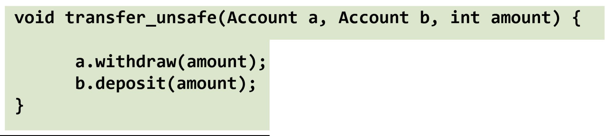
Problem: the transfer does
not happen atomically, i.e. another thread may
observe the withdraw but not (yet) the deposit.
Back
ETH::2._Semester::PProg::12._Linearizability_and_TM::5._Transactional_Memory_Motivation
Bank transfer without protection:
Problem: the transfer does
not happen atomically, i.e. another thread may
observe the withdraw but not (yet) the deposit.
Individual synchronized methods make each operation atomic by itself, but not their composition. Composing several thread-safe operations is exactly what atomic blocks are meant to provide.
Field-by-field Comparison
| Field |
Before |
After |
| Text |
|
Bank transfer without protection: <br><br><img src="paste-e991d7605087f01664a66b4c3a63e3eca882d96b.jpg"><br><br>Problem: the transfer does {{c1::not happen atomically}}, i.e. another thread may {{c1::observe the withdraw but not (yet) the deposit}}. |
| Extra |
|
Individual synchronized methods make each operation atomic by itself, but not their composition. Composing several thread-safe operations is exactly what atomic blocks are meant to provide. |
Tags:
ETH::2._Semester::PProg::12._Linearizability_and_TM::5._Transactional_Memory_Motivation
Note 179: ETH::2. Semester::PProg
Deck: ETH::2. Semester::PProg
Note Type: Horvath Cloze
GUID: }j}d*P2~.?
added
Previous
Note did not exist
New Note
Front
ETH::2._Semester::PProg::12._Linearizability_and_TM::7._Conflicts_and_Implementation
Reference-based STM (the model discussed in the lecture): mutable state is put into special variables (Refs), which can only be modified inside a transaction. Everything else is immutable or not shared.
Back
ETH::2._Semester::PProg::12._Linearizability_and_TM::7._Conflicts_and_Implementation
Reference-based STM (the model discussed in the lecture): mutable state is put into special variables (Refs), which can only be modified inside a transaction. Everything else is immutable or not shared.
The alternative would be to protect all program variables (easier porting, but hard to implement since every memory operation must be checked). Refs restrict the checking to explicitly marked variables.
Field-by-field Comparison
| Field |
Before |
After |
| Text |
|
Reference-based STM (the model discussed in the lecture): mutable state is put into {{c1::special variables (Refs)}}, which {{c2::can only be modified inside a transaction}}. Everything else is {{c3::immutable or not shared}}. |
| Extra |
|
The alternative would be to protect all program variables (easier porting, but hard to implement since every memory operation must be checked). Refs restrict the checking to explicitly marked variables. |
Tags:
ETH::2._Semester::PProg::12._Linearizability_and_TM::7._Conflicts_and_Implementation
Note 180: ETH::2. Semester::PProg
Deck: ETH::2. Semester::PProg
Note Type: Horvath Cloze
GUID: ~x[|;#m8/<
added
Previous
Note did not exist
New Note
Front
ETH::2._Semester::PProg::11._Lock_Free_Programming::6._Hazard_Pointers
Hazard-pointer idea.
The ABA problem stems from reusing a pointer \(P\) that thread \(X\) has read but not yet CAS-written, while another thread \(Y\) modifies it meanwhile.
To prevent reuse:
- before \(X\) reads \(P\), it marks \(P\) hazardous by writing it into its slot of an array (one slot per thread) associated with the data structure;
- when finished (after the CAS), \(X\) removes \(P\) from the array (sets its slot back to null);
- before \(Y\) reuses \(P\), it checks all entries of the hazard array and only reuses \(P\) if it is not hazardous.
Back
ETH::2._Semester::PProg::11._Lock_Free_Programming::6._Hazard_Pointers
Hazard-pointer idea.
The ABA problem stems from reusing a pointer \(P\) that thread \(X\) has read but not yet CAS-written, while another thread \(Y\) modifies it meanwhile.
To prevent reuse:
- before \(X\) reads \(P\), it marks \(P\) hazardous by writing it into its slot of an array (one slot per thread) associated with the data structure;
- when finished (after the CAS), \(X\) removes \(P\) from the array (sets its slot back to null);
- before \(Y\) reuses \(P\), it checks all entries of the hazard array and only reuses \(P\) if it is not hazardous.
The hazard array has \(n\) = number-of-threads slots. A node is reusable only when no thread has it flagged as hazardous.
Field-by-field Comparison
| Field |
Before |
After |
| Text |
|
Hazard-pointer idea. <br>The ABA problem stems from reusing a pointer \(P\) that thread \(X\) has read but not yet CAS-written, while another thread \(Y\) modifies it meanwhile. <br>To prevent reuse: <ol><li>before \(X\) reads \(P\), it {{c1::marks \(P\) hazardous by writing it into its slot of an array (one slot per thread) associated with the data structure}};</li><li>when finished (after the CAS), \(X\) {{c2::removes \(P\) from the array (sets its slot back to null)}};</li><li>before \(Y\) reuses \(P\), it {{c3::checks all entries of the hazard array and only reuses \(P\) if it is not hazardous}}.</li></ol> |
| Extra |
|
The hazard array has \(n\) = number-of-threads slots. A node is reusable only when no thread has it flagged as hazardous. |
Tags:
ETH::2._Semester::PProg::11._Lock_Free_Programming::6._Hazard_Pointers