\(g \geq \Omega(f)\) \( \Leftrightarrow\) \( f \leq O(g)\)
Note 1: ETH::1. Semester::A&D
Deck: ETH::1. Semester::A&D
Note Type: Horvath Cloze
GUID:
deleted
Note Type: Horvath Cloze
GUID:
A!-/#G=){
Deleted Note
Front
Back
\(g \geq \Omega(f)\) \( \Leftrightarrow\) \( f \leq O(g)\)
Current
Note has been deleted
Field-by-field Comparison
| Field | Before | After |
|---|---|---|
| Text |
Note 2: ETH::1. Semester::A&D
Deck: ETH::1. Semester::A&D
Note Type: Horvath Cloze
GUID:
deleted
Note Type: Horvath Cloze
GUID:
A+lafWP/s]
Deleted Note
Front
In a directed graph we call a (\(\epsilon\)/Eulerian/Hamiltonian) walk/closed walk/path/cycle a directed (gerichtet) (\(\epsilon\)/Eulerian/Hamiltonian) walk/closed walk/path/cycle.
Back
In a directed graph we call a (\(\epsilon\)/Eulerian/Hamiltonian) walk/closed walk/path/cycle a directed (gerichtet) (\(\epsilon\)/Eulerian/Hamiltonian) walk/closed walk/path/cycle.
Current
Note has been deleted
Field-by-field Comparison
| Field | Before | After |
|---|---|---|
| Text |
Note 3: ETH::1. Semester::A&D
Deck: ETH::1. Semester::A&D
Note Type: Horvath Reverso
GUID:
deleted
Note Type: Horvath Reverso
GUID:
A1y[0:/g)f
Deleted Note
Front
Closed Walk
Back
Closed Walk
Zyklus
Current
Note has been deleted
Field-by-field Comparison
| Field | Before | After |
|---|---|---|
| Front | ||
| Back |
Note 4: ETH::1. Semester::A&D
Deck: ETH::1. Semester::A&D
Note Type: Horvath Classic
GUID:
deleted
Note Type: Horvath Classic
GUID:
A8P;P^G,v4
Deleted Note
Front
Runtime of sorting an array containing only \(1, 0\)?
Back
Runtime of sorting an array containing only \(1, 0\)?
Using bucketsort, we can achieve \(O(n)\).
We go through the array once, counting occurences of \(0\) as x. We then add \(x\) zeros in the beginning and fill the rest with 1s.
We go through the array once, counting occurences of \(0\) as x. We then add \(x\) zeros in the beginning and fill the rest with 1s.
Current
Note has been deleted
Field-by-field Comparison
| Field | Before | After |
|---|---|---|
| Front | ||
| Back |
Note 5: ETH::1. Semester::A&D
Deck: ETH::1. Semester::A&D
Note Type: Algorithms
GUID:
deleted
Note Type: Algorithms
GUID:
AJT5T7qaW3
Deleted Note
Front
Runtime of Find Closed Eulerian Path?
Back
Runtime of Find Closed Eulerian Path?
\(O(n+m)\)
In an Adjacency Matrix: runtime is \(O(n^2)\) as looping over all edges is \(O(n)\).
In an Adjacency List: we loop \(n\) times over \(O(1 + \deg(u))\).
Using the handshake lemma: \(\sum_{u \in V} (1 + \deg(u)) = n + \sum_{u \in V} \deg(u) = n + 2m\)
In an Adjacency Matrix: runtime is \(O(n^2)\) as looping over all edges is \(O(n)\).
In an Adjacency List: we loop \(n\) times over \(O(1 + \deg(u))\).
Using the handshake lemma: \(\sum_{u \in V} (1 + \deg(u)) = n + \sum_{u \in V} \deg(u) = n + 2m\)
Current
Note has been deleted
Field-by-field Comparison
| Field | Before | After |
|---|---|---|
| Name | ||
| Runtime | ||
| Approach | ||
| Pseudocode | ||
| Extra Info |
Note 6: ETH::1. Semester::A&D
Deck: ETH::1. Semester::A&D
Note Type: Horvath Cloze
GUID:
deleted
Note Type: Horvath Cloze
GUID:
AQQfmx,sQF
Deleted Note
Front
A graph \(G\) is acyclic (azyklisch) if it has no cycles (Kreise).
Back
A graph \(G\) is acyclic (azyklisch) if it has no cycles (Kreise).
Current
Note has been deleted
Field-by-field Comparison
| Field | Before | After |
|---|---|---|
| Text |
Note 7: ETH::1. Semester::A&D
Deck: ETH::1. Semester::A&D
Note Type: Horvath Cloze
GUID:
deleted
Note Type: Horvath Cloze
GUID:
AS{7LiImd:
Deleted Note
Front
A graph \(G\) is bipartite if {{c2:: it's possible to partition the vertices into two sets \(V_1\) and \(V_2\) that are disjoint and cover the graph. Any edge \(\{u, v\}\) has to have one endpoint in \(V_1\) and the other in \(V_2\)}}.
Back
A graph \(G\) is bipartite if {{c2:: it's possible to partition the vertices into two sets \(V_1\) and \(V_2\) that are disjoint and cover the graph. Any edge \(\{u, v\}\) has to have one endpoint in \(V_1\) and the other in \(V_2\)}}.
Current
Note has been deleted
Field-by-field Comparison
| Field | Before | After |
|---|---|---|
| Text |
Note 8: ETH::1. Semester::A&D
Deck: ETH::1. Semester::A&D
Note Type: Horvath Cloze
GUID:
deleted
Note Type: Horvath Cloze
GUID:
AY}!l[d)1z
Deleted Note
Front
Name the impossible cases in DFS pre/post ordering for edge \((u, v)\):
- Overlapping but not nested intervals:
- {{c2:: \(\text{pre}(u)<\text{pre}(v)<\text{post}(u)<\text{post}(v)\): As visit(u) would call visit(v) before the recursive call ends.
 }}
}}
Back
Name the impossible cases in DFS pre/post ordering for edge \((u, v)\):
- Overlapping but not nested intervals:
- {{c2:: \(\text{pre}(u)<\text{pre}(v)<\text{post}(u)<\text{post}(v)\): As visit(u) would call visit(v) before the recursive call ends. }}
Current
Note has been deleted
Field-by-field Comparison
| Field | Before | After |
|---|---|---|
| Text |
Note 9: ETH::1. Semester::A&D
Deck: ETH::1. Semester::A&D
Note Type: Algorithms
GUID:
deleted
Note Type: Algorithms
GUID:
Ah4U@kYYNJ
Deleted Note
Front
Runtime of Linear Search?
Back
Runtime of Linear Search?
\(\Theta(n)\) as we go through the entire list once.
Current
Note has been deleted
Field-by-field Comparison
| Field | Before | After |
|---|---|---|
| Name | ||
| Runtime | ||
| Requirements | ||
| Approach |
Note 10: ETH::1. Semester::A&D
Deck: ETH::1. Semester::A&D
Note Type: Horvath Cloze
GUID:
deleted
Note Type: Horvath Cloze
GUID:
Ah6X9iA&#j
Deleted Note
Front
The ADT stack has the following operations:
- push(k, S): push a new object k to the top of the stack S
- pop(S): remove and return the top element of the stack S
- top(S): get the top element of the stack S without deleting it
Back
The ADT stack has the following operations:
- push(k, S): push a new object k to the top of the stack S
- pop(S): remove and return the top element of the stack S
- top(S): get the top element of the stack S without deleting it
Other operations might be isEmpty or emptystack which produces and emtpy stack.
Current
Note has been deleted
Field-by-field Comparison
| Field | Before | After |
|---|---|---|
| Text | ||
| Extra |
Note 11: ETH::1. Semester::A&D
Deck: ETH::1. Semester::A&D
Note Type: Horvath Classic
GUID:
deleted
Note Type: Horvath Classic
GUID:
AqQ}Ty8GRj
Deleted Note
Front
How do we fix the Quicksort worst-case runtime?
Back
How do we fix the Quicksort worst-case runtime?
Chose a random element as the pivot.
Median of medians algo ideal but too complex to implement.
Median of medians algo ideal but too complex to implement.
Current
Note has been deleted
Field-by-field Comparison
| Field | Before | After |
|---|---|---|
| Front | ||
| Back |
Note 12: ETH::1. Semester::A&D
Deck: ETH::1. Semester::A&D
Note Type: Horvath Cloze
GUID:
deleted
Note Type: Horvath Cloze
GUID:
Au,kdh[/@(
Deleted Note
Front
A safe edge is an edge that is included in at all MSTs.
Back
A safe edge is an edge that is included in at all MSTs.
all, If the edge-weights are distinct, which means there is one unique MST.
Current
Note has been deleted
Field-by-field Comparison
| Field | Before | After |
|---|---|---|
| Text | ||
| Extra |
Note 13: ETH::1. Semester::A&D
Deck: ETH::1. Semester::A&D
Note Type: Horvath Cloze
GUID:
deleted
Note Type: Horvath Cloze
GUID:
Auw]yKf@xT
Deleted Note
Front
Pre-/Post-Ordering Classification for an edge \((u, v)\):
\(\text{pre}(u) < \text{pre}(v) < \text{post}(v) < \text{post}(u)\), but not tree edge: Forward edge
\(\text{pre}(u) < \text{pre}(v) < \text{post}(v) < \text{post}(u)\), but not tree edge: Forward edge
Back
Pre-/Post-Ordering Classification for an edge \((u, v)\):
\(\text{pre}(u) < \text{pre}(v) < \text{post}(v) < \text{post}(u)\), but not tree edge: Forward edge
\(\text{pre}(u) < \text{pre}(v) < \text{post}(v) < \text{post}(u)\), but not tree edge: Forward edge
Current
Note has been deleted
Field-by-field Comparison
| Field | Before | After |
|---|---|---|
| Text |
Note 14: ETH::1. Semester::A&D
Deck: ETH::1. Semester::A&D
Note Type: Horvath Classic
GUID:
deleted
Note Type: Horvath Classic
GUID:
B#Jj9:E=8j
Deleted Note
Front
Cut and Paste Proof of Cut-Property:
Back
Cut and Paste Proof of Cut-Property:
Let \((S, V \setminus S)\) be any cut of a graph \(G\).
Let \(e = (u,v)\) be the minimal edge crossing this cut.
We want to show that \(e \in T\).
- Assume \(e \not \in T\) for contradiction.
- Since \(T\) is a spanning tree, \(T \cup {u}\) contains a cycle, crossing the cut at least twice (once via \(e\) and once via another edge \(e’\).)
- We now construct \(T’= (T \cup {e}) \setminus {e’}\) which breaks the cycle but keeps the MST property.
- Since \(w(e) < w(e’)\), \(w(T’) < w(T)\) and thus \(T\) is not an MST.
Current
Note has been deleted
Field-by-field Comparison
| Field | Before | After |
|---|---|---|
| Front | ||
| Back |
Note 15: ETH::1. Semester::A&D
Deck: ETH::1. Semester::A&D
Note Type: Horvath Classic
GUID:
deleted
Note Type: Horvath Classic
GUID:
B)ghZbgf?6
Deleted Note
Front
Describe the steps of Prim's Algorithm:
Back
Describe the steps of Prim's Algorithm:
Prim’s algorithm starts with a single vertex and grows the MST outwards from that seed.
- Initialisation:
- Select and arbitrary starting vertex \(s\) and empty set \(F\)
- Set \(S = {s}\) tracks the vertices in the MST
- Each vertex gets a
key[v] =representing the cheapest known connection cost to \(v\):- \(\infty\) if no edge connects \(s\) to \(v\)
- \(w(s, v)\) if edge \((s, v)\) exists
- Use a priority queue \(Q\) (Min-Heap) to store the vertices, in order of lowest
keycost
- Iteration:
- Select and add Extract the vertex \(u\) with the minimum
keyfrom \(Q\). This is the cheapest to connected to the current MST. Add \(u\) to \(S\). - Update Neighbours For each neighbour \(v\) of \(u\) not in \(S\):
- If \(w(u, v) < \text{key}[v]\) update
key[v] = w(u, v)and update the priority in $Q$.- This discovers potentially cheaper connections to vertices outside the current MST. If a cheaper edge to \(v\) is found, the current value in
key[v]cannot be part of the MST
- This discovers potentially cheaper connections to vertices outside the current MST. If a cheaper edge to \(v\) is found, the current value in
- If \(w(u, v) < \text{key}[v]\) update
- Select and add Extract the vertex \(u\) with the minimum
- Termination: When \(Q\) is empty, all vertices are in \(S\) and connected, and the edges chosen are in the MST (tracked in the set \(F\) through updates).
Current
Note has been deleted
Field-by-field Comparison
| Field | Before | After |
|---|---|---|
| Front | ||
| Back |
Note 16: ETH::1. Semester::A&D
Deck: ETH::1. Semester::A&D
Note Type: Horvath Reverso
GUID:
deleted
Note Type: Horvath Reverso
GUID:
B+m&Yt;~bM
Deleted Note
Front
Path
Back
Path
Pfad
Current
Note has been deleted
Field-by-field Comparison
| Field | Before | After |
|---|---|---|
| Front | ||
| Back |
Note 17: ETH::1. Semester::A&D
Deck: ETH::1. Semester::A&D
Note Type: Horvath Cloze
GUID:
deleted
Note Type: Horvath Cloze
GUID:
B/7aNL0zYE
Deleted Note
Front
Boruvka's Algorithm has a runtime of \(O((|V| + |E|) \log |V|)\).
Back
Boruvka's Algorithm has a runtime of \(O((|V| + |E|) \log |V|)\).
During each iteration, we examine all edges to find the cheapest one: \(O(|V| + |E|)\):
- Run DFS to find the connected components (ZHKs): \(O(|V| + |E|)\)
- Find the cheapest one \(O(|E|)\)
Current
Note has been deleted
Field-by-field Comparison
| Field | Before | After |
|---|---|---|
| Text | ||
| Extra |
Note 18: ETH::1. Semester::A&D
Deck: ETH::1. Semester::A&D
Note Type: Horvath Cloze
GUID:
deleted
Note Type: Horvath Cloze
GUID:
B9BorfLC*u
Deleted Note
Front
{{c1:: \(\sum_{i = 1}^{n} i\)::Sum}} \(\leq\) \(O(n^2)\)
Back
{{c1:: \(\sum_{i = 1}^{n} i\)::Sum}} \(\leq\) \(O(n^2)\)
Current
Note has been deleted
Field-by-field Comparison
| Field | Before | After |
|---|---|---|
| Text |
Note 19: ETH::1. Semester::A&D
Deck: ETH::1. Semester::A&D
Note Type: Algorithms
GUID:
deleted
Note Type: Algorithms
GUID:
BRmyi3>lm%
Deleted Note
Front
Back
Runtime of
DFS
Runtime: {{c1::\( \mathcal{O}(|E| + |V|) \)}}
Approach:
Uses:
?Current
Note has been deleted
Field-by-field Comparison
| Field | Before | After |
|---|---|---|
| Name |
Note 20: ETH::1. Semester::A&D
Deck: ETH::1. Semester::A&D
Note Type: Horvath Cloze
GUID:
deleted
Note Type: Horvath Cloze
GUID:
Bb-m%-jtI|
Deleted Note
Front
Pre-/Post-Ordering classification for an edge \((u, v)\):
\(\text{pre}(v) < \text{post}(v) < \text{pre}(u) < \text{post}(u)\): Cross edge, \(u, v\) in different subtrees
\(\text{pre}(v) < \text{post}(v) < \text{pre}(u) < \text{post}(u)\): Cross edge, \(u, v\) in different subtrees
Back
Pre-/Post-Ordering classification for an edge \((u, v)\):
\(\text{pre}(v) < \text{post}(v) < \text{pre}(u) < \text{post}(u)\): Cross edge, \(u, v\) in different subtrees
\(\text{pre}(v) < \text{post}(v) < \text{pre}(u) < \text{post}(u)\): Cross edge, \(u, v\) in different subtrees
Current
Note has been deleted
Field-by-field Comparison
| Field | Before | After |
|---|---|---|
| Text |
Note 21: ETH::1. Semester::A&D
Deck: ETH::1. Semester::A&D
Note Type: Horvath Cloze
GUID:
deleted
Note Type: Horvath Cloze
GUID:
Bgd/GP4-Fq
Deleted Note
Front
A graph \(G\) is a tree if it is connected and has no cycles (Kreise).
Back
A graph \(G\) is a tree if it is connected and has no cycles (Kreise).
Current
Note has been deleted
Field-by-field Comparison
| Field | Before | After |
|---|---|---|
| Text |
Note 22: ETH::1. Semester::A&D
Deck: ETH::1. Semester::A&D
Note Type: Horvath Classic
GUID:
deleted
Note Type: Horvath Classic
GUID:
Bq5(?)1v6(
Deleted Note
Front
What does \(\prod_{i=1}^n a_i\) mean?
Back
What does \(\prod_{i=1}^n a_i\) mean?
It is the product of all numbers between \(i\) and \(n\), in this specific case it is \(n!\).
Current
Note has been deleted
Field-by-field Comparison
| Field | Before | After |
|---|---|---|
| Front | ||
| Back |
Note 23: ETH::1. Semester::A&D
Deck: ETH::1. Semester::A&D
Note Type: Horvath Cloze
GUID:
deleted
Note Type: Horvath Cloze
GUID:
Br&58pkCU{
Deleted Note
Front
We start counting the height of a tree at \(0\).
Back
We start counting the height of a tree at \(0\).
Current
Note has been deleted
Field-by-field Comparison
| Field | Before | After |
|---|---|---|
| Text |
Note 24: ETH::1. Semester::A&D
Deck: ETH::1. Semester::A&D
Note Type: Horvath Cloze
GUID:
deleted
Note Type: Horvath Cloze
GUID:
BvQCv]T&c0
Deleted Note
Front
Choose a tight bound!
\(O(\log(n!))\leq O(n \log(n))\)
\(O(\log(n!))\leq O(n \log(n))\)
Back
Choose a tight bound!
\(O(\log(n!))\leq O(n \log(n))\)
\(O(\log(n!))\leq O(n \log(n))\)
Current
Note has been deleted
Field-by-field Comparison
| Field | Before | After |
|---|---|---|
| Text |
Note 25: ETH::1. Semester::A&D
Deck: ETH::1. Semester::A&D
Note Type: Horvath Cloze
GUID:
deleted
Note Type: Horvath Cloze
GUID:
BwR)%}KG6h
Deleted Note
Front
Boruvka's Algorithm requires an undirected, connected, weighted Graph.
Back
Boruvka's Algorithm requires an undirected, connected, weighted Graph.
Current
Note has been deleted
Field-by-field Comparison
| Field | Before | After |
|---|---|---|
| Text |
Note 26: ETH::1. Semester::A&D
Deck: ETH::1. Semester::A&D
Note Type: Horvath Cloze
GUID:
deleted
Note Type: Horvath Cloze
GUID:
Bz)mOB:[n-
Deleted Note
Front
2-3 Tree: The runtime of search, insertion and deletion is \(O(\log n)\).
Back
2-3 Tree: The runtime of search, insertion and deletion is \(O(\log n)\).
This is because the tree is now forced to be balanced and \(h \leq \log_2 n\).
Current
Note has been deleted
Field-by-field Comparison
| Field | Before | After |
|---|---|---|
| Text | ||
| Extra |
Note 27: ETH::1. Semester::A&D
Deck: ETH::1. Semester::A&D
Note Type: Algorithms
GUID:
deleted
Note Type: Algorithms
GUID:
C$#TvbwG_l
Deleted Note
Front
Runtime of Longest Ascending Subsequence (Längste Aufsteigende Teilfolge)?
Back
Runtime of Longest Ascending Subsequence (Längste Aufsteigende Teilfolge)?
\(\Theta(n \log n)\)
Current
Note has been deleted
Field-by-field Comparison
| Field | Before | After |
|---|---|---|
| Name | ||
| Runtime | ||
| Approach | ||
| Pseudocode |
Note 28: ETH::1. Semester::A&D
Deck: ETH::1. Semester::A&D
Note Type: Horvath Cloze
GUID:
deleted
Note Type: Horvath Cloze
GUID:
C1$vvwFoR0
Deleted Note
Front
In graph theory, a closed Eulerian walk (Eulerzyklus) is an Eulerian walk (Eulerweg) that ends at the start vertex.
Back
In graph theory, a closed Eulerian walk (Eulerzyklus) is an Eulerian walk (Eulerweg) that ends at the start vertex.
Current
Note has been deleted
Field-by-field Comparison
| Field | Before | After |
|---|---|---|
| Text |
Note 29: ETH::1. Semester::A&D
Deck: ETH::1. Semester::A&D
Note Type: Horvath Classic
GUID:
deleted
Note Type: Horvath Classic
GUID:
C5BRbDI3JL
Deleted Note
Front
j = 1
while j <= n do
j = 2j
f()
Back
j = 1
while j <= n do
j = 2j
f()
\[\sum_{j = 0}^{\lfloor \log_2 n \rfloor}\]
We go from \(0\) to \(\lfloor \log_2 n \rfloor\) not from \(1\).
Current
Note has been deleted
Field-by-field Comparison
| Field | Before | After |
|---|---|---|
| Front | ||
| Back |
Note 30: ETH::1. Semester::A&D
Deck: ETH::1. Semester::A&D
Note Type: Horvath Cloze
GUID:
deleted
Note Type: Horvath Cloze
GUID:
C9v-$JhadV
Deleted Note
Front
If \(\frac{f(n)}{g(n)}\) tends to 0, then \(f \leq O(g)\) and \(f \neq \Theta(g)\)
Back
If \(\frac{f(n)}{g(n)}\) tends to 0, then \(f \leq O(g)\) and \(f \neq \Theta(g)\)
Current
Note has been deleted
Field-by-field Comparison
| Field | Before | After |
|---|---|---|
| Text |
Note 31: ETH::1. Semester::A&D
Deck: ETH::1. Semester::A&D
Note Type: Horvath Classic
GUID:
deleted
Note Type: Horvath Classic
GUID:
CJsa&>C5sO
Deleted Note
Front
Can Kruskal's Algorithm be executed in \(O(|E| + |V|\log|V|)\) time?
Back
Can Kruskal's Algorithm be executed in \(O(|E| + |V|\log|V|)\) time?
No, we need to sort the edges which takes at least \(|E| \log |E|\) time.
Current
Note has been deleted
Field-by-field Comparison
| Field | Before | After |
|---|---|---|
| Front | ||
| Back |
Note 32: ETH::1. Semester::A&D
Deck: ETH::1. Semester::A&D
Note Type: Horvath Cloze
GUID:
deleted
Note Type: Horvath Cloze
GUID:
CaRvZ82Z-e
Deleted Note
Front
{{c1:: \(\sum_{i = 1}^{n} \sum_{i = 1}^{n} \sum_{i = 1}^{n} 1\)::Sum}} \(=\) \(n^3\)
Back
{{c1:: \(\sum_{i = 1}^{n} \sum_{i = 1}^{n} \sum_{i = 1}^{n} 1\)::Sum}} \(=\) \(n^3\)
Current
Note has been deleted
Field-by-field Comparison
| Field | Before | After |
|---|---|---|
| Text |
Note 33: ETH::1. Semester::A&D
Deck: ETH::1. Semester::A&D
Note Type: Horvath Cloze
GUID:
deleted
Note Type: Horvath Cloze
GUID:
Ceyt5d#^?A
Deleted Note
Front
\( g = \Theta(f)\) \(\Leftrightarrow\) {{c1:: \(g \leq O(f) \text{ and } f \leq O(g)\)}}
Back
\( g = \Theta(f)\) \(\Leftrightarrow\) {{c1:: \(g \leq O(f) \text{ and } f \leq O(g)\)}}
Current
Note has been deleted
Field-by-field Comparison
| Field | Before | After |
|---|---|---|
| Text |
Note 34: ETH::1. Semester::A&D
Deck: ETH::1. Semester::A&D
Note Type: Horvath Classic
GUID:
deleted
Note Type: Horvath Classic
GUID:
Cnkg?3]K
Deleted Note
Front
Quicksort space complexity?
Back
Quicksort space complexity?
\(O(n)\)
Current
Note has been deleted
Field-by-field Comparison
| Field | Before | After |
|---|---|---|
| Front | ||
| Back |
Note 35: ETH::1. Semester::A&D
Deck: ETH::1. Semester::A&D
Note Type: Horvath Classic
GUID:
deleted
Note Type: Horvath Classic
GUID:
Cz/kys?.PN
Deleted Note
Front
Every undirected graph that contains a Hamilton path also contains an eulerian walk?
Back
Every undirected graph that contains a Hamilton path also contains an eulerian walk?
No.
Current
Note has been deleted
Field-by-field Comparison
| Field | Before | After |
|---|---|---|
| Front | ||
| Back |
Note 36: ETH::1. Semester::A&D
Deck: ETH::1. Semester::A&D
Note Type: Horvath Cloze
GUID:
deleted
Note Type: Horvath Cloze
GUID:
C}:U@+B*;Q
Deleted Note
Front
{{c1:: \(\sum_{i = 1}^{n} i^3\)::Sum}} \(\leq\) \(O(n^4)\)
Back
{{c1:: \(\sum_{i = 1}^{n} i^3\)::Sum}} \(\leq\) \(O(n^4)\)
Current
Note has been deleted
Field-by-field Comparison
| Field | Before | After |
|---|---|---|
| Text |
Note 37: ETH::1. Semester::A&D
Deck: ETH::1. Semester::A&D
Note Type: Horvath Cloze
GUID:
deleted
Note Type: Horvath Cloze
GUID:
D!4=n6GM2_
Deleted Note
Front
In a doubly linked list, we store a pointer to the previous and next element for each key.
This increases memory usage as a trade-off for speed.
This increases memory usage as a trade-off for speed.
Back
In a doubly linked list, we store a pointer to the previous and next element for each key.
This increases memory usage as a trade-off for speed.
This increases memory usage as a trade-off for speed.
Current
Note has been deleted
Field-by-field Comparison
| Field | Before | After |
|---|---|---|
| Text |
Note 38: ETH::1. Semester::A&D
Deck: ETH::1. Semester::A&D
Note Type: Horvath Classic
GUID:
deleted
Note Type: Horvath Classic
GUID:
D%cpEp.*I3
Deleted Note
Front
What is l'Hôpital's Rule?
Back
What is l'Hôpital's Rule?
If \(\lim_{x \to \infty} f(x) = \lim_{x \to \infty} g(x) = \infty\) (or both \(=0\)), and \(\lim_{x \to \infty} \frac{f'(x)}{g'(x)}\) exists (or is \(\pm\infty\)), then:
\(\lim_{x \to \infty} \frac{f(x)}{g(x)} = \lim_{x \to \infty} \frac{f'(x)}{g'(x)}\)
Current
Note has been deleted
Field-by-field Comparison
| Field | Before | After |
|---|---|---|
| Front | ||
| Back |
Note 39: ETH::1. Semester::A&D
Deck: ETH::1. Semester::A&D
Note Type: Horvath Cloze
GUID:
deleted
Note Type: Horvath Cloze
GUID:
D2>~h
Deleted Note
Front
The ADT queue has the following operations:
- enqueue(k, S): append at the end of the queue
- dequeue(S): remove and return the first element of the queue
Back
The ADT queue has the following operations:
- enqueue(k, S): append at the end of the queue
- dequeue(S): remove and return the first element of the queue
Current
Note has been deleted
Field-by-field Comparison
| Field | Before | After |
|---|---|---|
| Text |
Note 40: ETH::1. Semester::A&D
Deck: ETH::1. Semester::A&D
Note Type: Horvath Cloze
GUID:
deleted
Note Type: Horvath Cloze
GUID:
D9:.N,D17I
Deleted Note
Front
A graph \(G\) is called a directed acyclic graph (DAG) (gerichteter azyklischer Graph) if there is no directed cycles (gerichteter Kreis).
Back
A graph \(G\) is called a directed acyclic graph (DAG) (gerichteter azyklischer Graph) if there is no directed cycles (gerichteter Kreis).
Current
Note has been deleted
Field-by-field Comparison
| Field | Before | After |
|---|---|---|
| Text |
Note 41: ETH::1. Semester::A&D
Deck: ETH::1. Semester::A&D
Note Type: Algorithms
GUID:
deleted
Note Type: Algorithms
GUID:
DD]dBe%Sn|
Deleted Note
Front
Runtime of Binary Search?
Back
Runtime of Binary Search?
\(O(\log(n))\) (optimal)
Current
Note has been deleted
Field-by-field Comparison
| Field | Before | After |
|---|---|---|
| Name | ||
| Runtime | ||
| Requirements | ||
| Approach | ||
| Pseudocode |
Note 42: ETH::1. Semester::A&D
Deck: ETH::1. Semester::A&D
Note Type: Horvath Classic
GUID:
deleted
Note Type: Horvath Classic
GUID:
D]]~[I)jx9
Deleted Note
Front
What is the lower limit for sorting algorithms?
Back
What is the lower limit for sorting algorithms?
\(\Omega(n \log n)\) cannot be improved upon.
Current
Note has been deleted
Field-by-field Comparison
| Field | Before | After |
|---|---|---|
| Front | ||
| Back |
Note 43: ETH::1. Semester::A&D
Deck: ETH::1. Semester::A&D
Note Type: Horvath Cloze
GUID:
deleted
Note Type: Horvath Cloze
GUID:
Dc@O2/=Azj
Deleted Note
Front
The number of edges in an MST are \(|V| - 1\).
Back
The number of edges in an MST are \(|V| - 1\).
Otherwise we could remove one and it would still span the edges, thus the cost is not minimal.
Current
Note has been deleted
Field-by-field Comparison
| Field | Before | After |
|---|---|---|
| Text | ||
| Extra |
Note 44: ETH::1. Semester::A&D
Deck: ETH::1. Semester::A&D
Note Type: Algorithms
GUID:
deleted
Note Type: Algorithms
GUID:
DeJ!2ph{Al
Deleted Note
Front
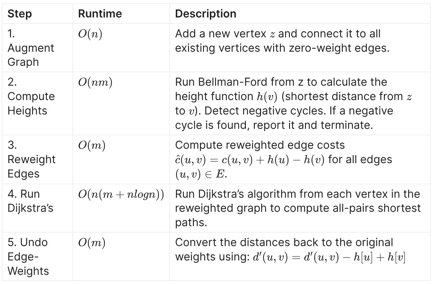
Runtime of Johnson's Algorithm?
Back
Runtime of Johnson's Algorithm?
\(O(|V| \cdot (|V| + |E|) \log |V|)\) (running dijkstra's n times, but allows negatives)
Current
Note has been deleted
Field-by-field Comparison
| Field | Before | After |
|---|---|---|
| Name | ||
| Runtime | ||
| Requirements | ||
| Approach | ||
| Use Case |
Note 45: ETH::1. Semester::A&D
Deck: ETH::1. Semester::A&D
Note Type: Horvath Cloze
GUID:
deleted
Note Type: Horvath Cloze
GUID:
DhNROhdDaL
Deleted Note
Front
A Minimum Spanning Tree is a subgraph of a connected, undirected, weighted graph that fullfills:
- spanning, it connects all vertices
- acylic, it's a tree
- minimal, the sum of all edge weights in the Tree is minimal
Back
A Minimum Spanning Tree is a subgraph of a connected, undirected, weighted graph that fullfills:
- spanning, it connects all vertices
- acylic, it's a tree
- minimal, the sum of all edge weights in the Tree is minimal
Current
Note has been deleted
Field-by-field Comparison
| Field | Before | After |
|---|---|---|
| Text |
Note 46: ETH::1. Semester::A&D
Deck: ETH::1. Semester::A&D
Note Type: Horvath Classic
GUID:
deleted
Note Type: Horvath Classic
GUID:
DkT;0O|rUB
Deleted Note
Front
What is \(\log x\) in AuD classes?
Back
What is \(\log x\) in AuD classes?
\(\log_2 x\)
Current
Note has been deleted
Field-by-field Comparison
| Field | Before | After |
|---|---|---|
| Front | ||
| Back |
Note 47: ETH::1. Semester::A&D
Deck: ETH::1. Semester::A&D
Note Type: Horvath Classic
GUID:
deleted
Note Type: Horvath Classic
GUID:
Dkf-+^.Z}
Deleted Note
Front
What does the Master theorem state when it comes to the upper bound on the asymptotic runtime of a function?
Back
What does the Master theorem state when it comes to the upper bound on the asymptotic runtime of a function?
Let \(a, C > 0\) and \(b \geq 0\) be constants and let \(T: \mathbb{N} \rightarrow \mathbb{R}^+\) a function such that for all even \(n \in \mathbb{N}\)
\(T(n) \leq aT(\frac{n}{2}) + Cn^b\).
Then for all \(n = 2^k\) the following statements hold:
1. if \(b > \log_2a\), \(T(n) \leq O(n^b)\)
2. if \(b = \log_2a\), \(T(n) \leq O(n^{log_2a}\log n)\)
3. if \(b < \log_2a\), \(T(n) \leq O(n^{\log_2a})\)
\(T(n) \leq aT(\frac{n}{2}) + Cn^b\).
Then for all \(n = 2^k\) the following statements hold:
1. if \(b > \log_2a\), \(T(n) \leq O(n^b)\)
2. if \(b = \log_2a\), \(T(n) \leq O(n^{log_2a}\log n)\)
3. if \(b < \log_2a\), \(T(n) \leq O(n^{\log_2a})\)
Current
Note has been deleted
Field-by-field Comparison
| Field | Before | After |
|---|---|---|
| Front | ||
| Back |
Note 48: ETH::1. Semester::A&D
Deck: ETH::1. Semester::A&D
Note Type: Horvath Cloze
GUID:
deleted
Note Type: Horvath Cloze
GUID:
Dn~?XXlS(X
Deleted Note
Front
We can run DFS in \(O(m)\) if we know the graph is connected, i.e. \(m \geq n - 1\).
Back
We can run DFS in \(O(m)\) if we know the graph is connected, i.e. \(m \geq n - 1\).
Current
Note has been deleted
Field-by-field Comparison
| Field | Before | After |
|---|---|---|
| Text |
Note 49: ETH::1. Semester::A&D
Deck: ETH::1. Semester::A&D
Note Type: Horvath Cloze
GUID:
deleted
Note Type: Horvath Cloze
GUID:
D{#5DM:PFn
Deleted Note
Front
Choose a tight bound!
\(O(1) \leq O(\log(n))\)
\(O(1) \leq O(\log(n))\)
Back
Choose a tight bound!
\(O(1) \leq O(\log(n))\)
\(O(1) \leq O(\log(n))\)
Current
Note has been deleted
Field-by-field Comparison
| Field | Before | After |
|---|---|---|
| Text |
Note 50: ETH::1. Semester::A&D
Deck: ETH::1. Semester::A&D
Note Type: Horvath Cloze
GUID:
deleted
Note Type: Horvath Cloze
GUID:
E%2HyUMa`
Deleted Note
Front
A graph \(G\) is connected (Zusammenhängend) if it has one connected component.
Back
A graph \(G\) is connected (Zusammenhängend) if it has one connected component.
Current
Note has been deleted
Field-by-field Comparison
| Field | Before | After |
|---|---|---|
| Text |
Note 51: ETH::1. Semester::A&D
Deck: ETH::1. Semester::A&D
Note Type: Horvath Cloze
GUID:
deleted
Note Type: Horvath Cloze
GUID:
E>+A_WABT2
Deleted Note
Front
{{c1:: \(\sum_{i = 1}^{n} i^3\)::Sum}} \(=\) {{c2::\(\frac{n^2(n + 1)^2}{4}\)}}
Back
{{c1:: \(\sum_{i = 1}^{n} i^3\)::Sum}} \(=\) {{c2::\(\frac{n^2(n + 1)^2}{4}\)}}
Current
Note has been deleted
Field-by-field Comparison
| Field | Before | After |
|---|---|---|
| Text |
Note 52: ETH::1. Semester::A&D
Deck: ETH::1. Semester::A&D
Note Type: Image Occlusion-73a2c
GUID:
deleted
Note Type: Image Occlusion-73a2c
GUID:
EE{ugGOkjL
Deleted Note
Front
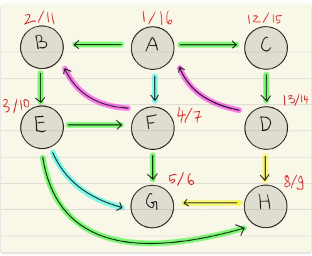
Back-, forward- or cross-edge?
Back
Back-, forward- or cross-edge?
Magenta: Back
Turquoise: Forward
Yellow: Cross
Turquoise: Forward
Yellow: Cross
Current
Note has been deleted
Field-by-field Comparison
| Field | Before | After |
|---|---|---|
| Occlusion | ||
| Image | ||
| Header | ||
| Back Extra |
Note 53: ETH::1. Semester::A&D
Deck: ETH::1. Semester::A&D
Note Type: Horvath Cloze
GUID:
deleted
Note Type: Horvath Cloze
GUID:
Ew6/RqtSN]
Deleted Note
Front
The {{c1::in-degree \(\deg_{\text{in} }(v)\) (Eingangsgrad)}} of a vertex in a directed graph is the number of edges that have \(v\) as the end-vertex.
Back
The {{c1::in-degree \(\deg_{\text{in} }(v)\) (Eingangsgrad)}} of a vertex in a directed graph is the number of edges that have \(v\) as the end-vertex.
Current
Note has been deleted
Field-by-field Comparison
| Field | Before | After |
|---|---|---|
| Text |
Note 54: ETH::1. Semester::A&D
Deck: ETH::1. Semester::A&D
Note Type: Horvath Cloze
GUID:
deleted
Note Type: Horvath Cloze
GUID:
F*Z7jn}vxk
Deleted Note
Front
The ADT List defines the following operations:
- insert(k, L): insert the key K at the end of the list L
- get(i, L): return the memory address of the i-th key in list L
- delete(k, L): remove the key k from the list L
- insertAfter(k, k', L): inserts the key k' after the key k in the list L
Back
The ADT List defines the following operations:
- insert(k, L): insert the key K at the end of the list L
- get(i, L): return the memory address of the i-th key in list L
- delete(k, L): remove the key k from the list L
- insertAfter(k, k', L): inserts the key k' after the key k in the list L
Current
Note has been deleted
Field-by-field Comparison
| Field | Before | After |
|---|---|---|
| Text |
Note 55: ETH::1. Semester::A&D
Deck: ETH::1. Semester::A&D
Note Type: Horvath Classic
GUID:
deleted
Note Type: Horvath Classic
GUID:
FAEpag8L6e
Deleted Note
Front
Runtime Determine if Hamiltonian path exists?
Back
Runtime Determine if Hamiltonian path exists?
Hamiltonian walk - exponential, we have to brute-force
Current
Note has been deleted
Field-by-field Comparison
| Field | Before | After |
|---|---|---|
| Front | ||
| Back |
Note 56: ETH::1. Semester::A&D
Deck: ETH::1. Semester::A&D
Note Type: Horvath Classic
GUID:
deleted
Note Type: Horvath Classic
GUID:
FG1IbvZ*6[
Deleted Note
Front
The depth \(h\) of a seach tree of any comparison-based algorithm satisfies which bound?
Back
The depth \(h\) of a seach tree of any comparison-based algorithm satisfies which bound?
\(h \geq \Omega(\log n)\) this is information theoretically the least amount of comparisons necessary.
Note that \(h \not \leq O(n)\) necessarily as we could have a really stupid algorithm that compares thrice for example.
Note that \(h \not \leq O(n)\) necessarily as we could have a really stupid algorithm that compares thrice for example.
Current
Note has been deleted
Field-by-field Comparison
| Field | Before | After |
|---|---|---|
| Front | ||
| Back |
Note 57: ETH::1. Semester::A&D
Deck: ETH::1. Semester::A&D
Note Type: Horvath Classic
GUID:
deleted
Note Type: Horvath Classic
GUID:
FS|421SN1o
Deleted Note
Front
Explain how union works in the optimised Union-Find:
Back
Explain how union works in the optimised Union-Find:
Arrays:
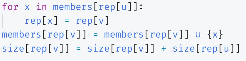
We update the reps, then the membership lists and finally the size.
- rep, where rep[v] gives the representative of \(v\).
- members, where members[rep[v]] which contains all members of the ZHK of \(v\)
- rank, where rank[rep[v]] contains the size of the ZHK of \(v\).
We always merge the smaller ZHK into the bigger to minimise updates.
We update the reps, then the membership lists and finally the size.
Current
Note has been deleted
Field-by-field Comparison
| Field | Before | After |
|---|---|---|
| Front | ||
| Back |
Note 58: ETH::1. Semester::A&D
Deck: ETH::1. Semester::A&D
Note Type: Horvath Classic
GUID:
deleted
Note Type: Horvath Classic
GUID:
FYr.:eNxT,
Deleted Note
Front
Types of 2-3 Tree nodes:
Back
Types of 2-3 Tree nodes:
Keys in left (middle, right) sub-tree \(l\) (\(m, r\) respect.ively):
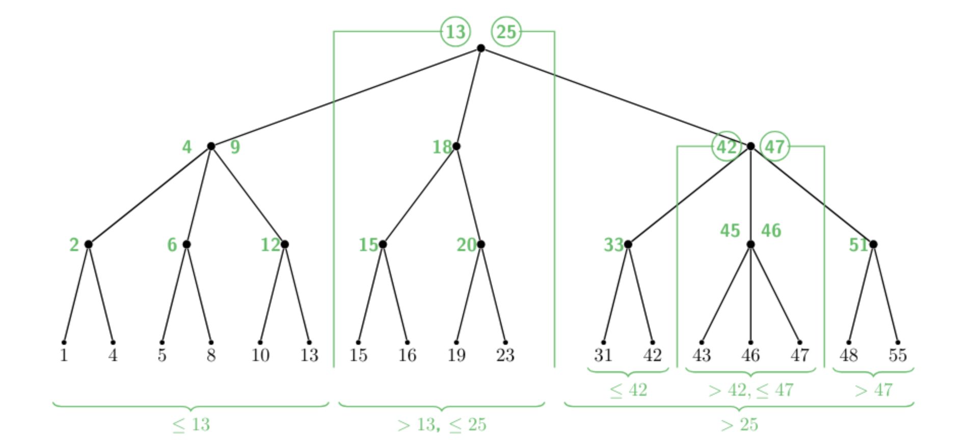
- 2 children: 1 separator \(s\) s.t. for \(l \leq s < r\).
- 3 children: 2 separators \(s_1, s_2\) s.t. \(l \leq s_1 < m \leq s_2 < r\)
Current
Note has been deleted
Field-by-field Comparison
| Field | Before | After |
|---|---|---|
| Front | ||
| Back |
Note 59: ETH::1. Semester::A&D
Deck: ETH::1. Semester::A&D
Note Type: Horvath Cloze
GUID:
deleted
Note Type: Horvath Cloze
GUID:
F^&OZQURkx
Deleted Note
Front
The ADT queue can be efficiently implemented using a singly linked list with a pointer to the end:
- push: \(O(1)\) insert at the end, with pointer to the end
- pop: \(O(1)\) remove the first element like in a stack
Back
The ADT queue can be efficiently implemented using a singly linked list with a pointer to the end:
- push: \(O(1)\) insert at the end, with pointer to the end
- pop: \(O(1)\) remove the first element like in a stack
Current
Note has been deleted
Field-by-field Comparison
| Field | Before | After |
|---|---|---|
| Text |
Note 60: ETH::1. Semester::A&D
Deck: ETH::1. Semester::A&D
Note Type: Algorithms
GUID:
deleted
Note Type: Algorithms
GUID:
F^nhYx>fXl
Deleted Note
Front
Back
Runtime of
Boruvka
Runtime:
Approach: Add all vertices to the set of components (so every vertex has its own component). As long as the size of the components set is greater than 1, connect each component to the one with the cheapest edge.
Uses: Find MST in weighted, undirected graph
?Current
Note has been deleted
Field-by-field Comparison
| Field | Before | After |
|---|---|---|
| Name | ||
| Approach |
Note 61: ETH::1. Semester::A&D
Deck: ETH::1. Semester::A&D
Note Type: Horvath Classic
GUID:
deleted
Note Type: Horvath Classic
GUID:
Fn+W}!cgj0
Deleted Note
Front
If we know that shortest paths have a length of max \(h\), runtime of algo to find them?
Back
If we know that shortest paths have a length of max \(h\), runtime of algo to find them?
We can find them in \(O(h|E|)\) using Bellman-Ford since we only need to relax \(h\) times.
Current
Note has been deleted
Field-by-field Comparison
| Field | Before | After |
|---|---|---|
| Front | ||
| Back |
Note 62: ETH::1. Semester::A&D
Deck: ETH::1. Semester::A&D
Note Type: Horvath Cloze
GUID:
deleted
Note Type: Horvath Cloze
GUID:
Fzt_!E{2Xk
Deleted Note
Front
Master Theorem: In \(T(n) \leq aT(n/2) + Cn^b\), \(Cn^b\) is the work done outside the recursive calls (\(\geq 0\)).
Back
Master Theorem: In \(T(n) \leq aT(n/2) + Cn^b\), \(Cn^b\) is the work done outside the recursive calls (\(\geq 0\)).
Current
Note has been deleted
Field-by-field Comparison
| Field | Before | After |
|---|---|---|
| Text |
Note 63: ETH::1. Semester::A&D
Deck: ETH::1. Semester::A&D
Note Type: Horvath Classic
GUID:
deleted
Note Type: Horvath Classic
GUID:
F{a&v[Q@_W
Deleted Note
Front
Let \(W\) be a walk and let \(u\) be a vertex, what is \(\text{deg}_W(u)\)? (generally)
Back
Let \(W\) be a walk and let \(u\) be a vertex, what is \(\text{deg}_W(u)\)? (generally)
The number of edges incident to \(u\) which are part of \(W\) but repetitions are included, therefore it is possible that \(\text{deg}(u) < \text{deg}_W(u)\).
Current
Note has been deleted
Field-by-field Comparison
| Field | Before | After |
|---|---|---|
| Front | ||
| Back |
Note 64: ETH::1. Semester::A&D
Deck: ETH::1. Semester::A&D
Note Type: Horvath Classic
GUID:
deleted
Note Type: Horvath Classic
GUID:
G9Xwk@MZZb
Deleted Note
Front
What does \(f \leq O(h)\) mean exactly?
Back
What does \(f \leq O(h)\) mean exactly?
\(\forall C > 0\) we have \(c \cdot f \leq O(h)\)
Current
Note has been deleted
Field-by-field Comparison
| Field | Before | After |
|---|---|---|
| Front | ||
| Back |
Note 65: ETH::1. Semester::A&D
Deck: ETH::1. Semester::A&D
Note Type: Horvath Cloze
GUID:
deleted
Note Type: Horvath Cloze
GUID:
G<9txw#|QX
Deleted Note
Front
The {{c1::out-degree \(\deg_{\text{out} }(v)\) (Ausgangsgrad)}} of a vertex in a directed graph is the number of edges that have \(v\) as the start-vertex.
Back
The {{c1::out-degree \(\deg_{\text{out} }(v)\) (Ausgangsgrad)}} of a vertex in a directed graph is the number of edges that have \(v\) as the start-vertex.
Current
Note has been deleted
Field-by-field Comparison
| Field | Before | After |
|---|---|---|
| Text |
Note 66: ETH::1. Semester::A&D
Deck: ETH::1. Semester::A&D
Note Type: Horvath Classic
GUID:
deleted
Note Type: Horvath Classic
GUID:
G?trbZc%;
Deleted Note
Front
What is a sufficient condition to show that \(f = \Theta(g)\)?
Back
What is a sufficient condition to show that \(f = \Theta(g)\)?
Let \(N\) be an infinite subset of \(\mathbb{N}\) and \(f: \mathbb{N} \rightarrow \mathbb{R}^+\) and \(g: \mathbb{N} \rightarrow \mathbb{R}^+\)
then \(\lim_{n\rightarrow \infty} \frac{f(n)}{g(n)} = C \in \mathbb{R}^+\) then \(f = \Theta(g)\)
then \(\lim_{n\rightarrow \infty} \frac{f(n)}{g(n)} = C \in \mathbb{R}^+\) then \(f = \Theta(g)\)
Current
Note has been deleted
Field-by-field Comparison
| Field | Before | After |
|---|---|---|
| Front | ||
| Back |
Note 67: ETH::1. Semester::A&D
Deck: ETH::1. Semester::A&D
Note Type: Horvath Cloze
GUID:
deleted
Note Type: Horvath Cloze
GUID:
GA*(aETcmb
Deleted Note
Front
Which datastructure is best for DFS?
In a sparse graph an adjacency list is better, in a dense graph an adjacency matrix is better.
In a sparse graph an adjacency list is better, in a dense graph an adjacency matrix is better.
Back
Which datastructure is best for DFS?
In a sparse graph an adjacency list is better, in a dense graph an adjacency matrix is better.
In a sparse graph an adjacency list is better, in a dense graph an adjacency matrix is better.
\(|E| \geq |V|^2 / 10\), then DFS has the same runtime in the worst-case using adjacency matrices or lists as \(|V| + |E| \leq |V| + |V|^2 \)which is \(O(n^2)\).
Current
Note has been deleted
Field-by-field Comparison
| Field | Before | After |
|---|---|---|
| Text | ||
| Extra |
Note 68: ETH::1. Semester::A&D
Deck: ETH::1. Semester::A&D
Note Type: Image Occlusion-73a2c
GUID:
deleted
Note Type: Image Occlusion-73a2c
GUID:
GKG~Tp?e4l
Deleted Note
Front
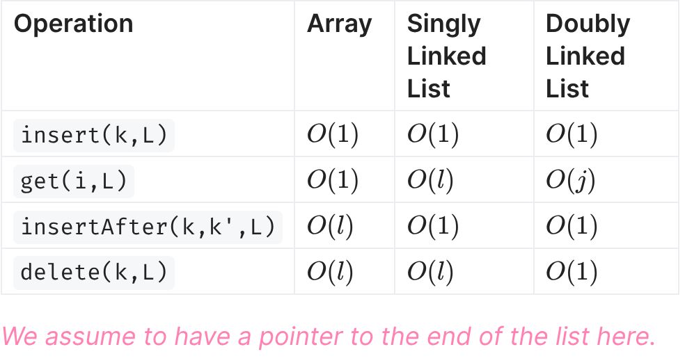
Note that the key parameter of insertAfter and delete in lists refers to the actual node, not it's value.
Back
Note that the key parameter of insertAfter and delete in lists refers to the actual node, not it's value.
Current
Note has been deleted
Field-by-field Comparison
| Field | Before | After |
|---|---|---|
| Occlusion | ||
| Image | ||
| Header |
Note 69: ETH::1. Semester::A&D
Deck: ETH::1. Semester::A&D
Note Type: Horvath Classic
GUID:
deleted
Note Type: Horvath Classic
GUID:
Gr6wW?Nt0R
Deleted Note
Front
How is a binary tree stored in memory? What are the indices of the children for a parent index \(k\)?
Back
How is a binary tree stored in memory? What are the indices of the children for a parent index \(k\)?
The children of a node k in a tree are at \(2k\) and \(2k + 1\).
This means that the tree is stored in memory by levels.
This means that the tree is stored in memory by levels.
Current
Note has been deleted
Field-by-field Comparison
| Field | Before | After |
|---|---|---|
| Front | ||
| Back |
Note 70: ETH::1. Semester::A&D
Deck: ETH::1. Semester::A&D
Note Type: Horvath Cloze
GUID:
deleted
Note Type: Horvath Cloze
GUID:
GsU2XikyZ:
Deleted Note
Front
We use Johnsons over Floyd-Warshall, when the graph is sparse, like in a tree.
Back
We use Johnsons over Floyd-Warshall, when the graph is sparse, like in a tree.
Then the \(|E|\) doesn't matter much in comparison to Floyd-Warshall's \(|V|^3\).
Current
Note has been deleted
Field-by-field Comparison
| Field | Before | After |
|---|---|---|
| Text | ||
| Extra |
Note 71: ETH::1. Semester::A&D
Deck: ETH::1. Semester::A&D
Note Type: Horvath Cloze
GUID:
deleted
Note Type: Horvath Cloze
GUID:
Gt4c53(i;/
Deleted Note
Front
In graph theory, a Hamiltonian path (Hamiltonpfad) is a path (Pfad) that contains every vertex (every vertex exactly once as it's a path).
Back
In graph theory, a Hamiltonian path (Hamiltonpfad) is a path (Pfad) that contains every vertex (every vertex exactly once as it's a path).
Current
Note has been deleted
Field-by-field Comparison
| Field | Before | After |
|---|---|---|
| Text |
Note 72: ETH::1. Semester::A&D
Deck: ETH::1. Semester::A&D
Note Type: Horvath Cloze
GUID:
deleted
Note Type: Horvath Cloze
GUID:
H0^#YREe-o
Deleted Note
Front
The 2-3 Trees we are covering in this course are external search-trees.
Back
The 2-3 Trees we are covering in this course are external search-trees.
This means that the values are stored in the leaves only. The nodes are for "navigation".
Current
Note has been deleted
Field-by-field Comparison
| Field | Before | After |
|---|---|---|
| Text | ||
| Extra |
Note 73: ETH::1. Semester::A&D
Deck: ETH::1. Semester::A&D
Note Type: Horvath Classic
GUID:
deleted
Note Type: Horvath Classic
GUID:
H>#zg]RQy9
Deleted Note
Front
Do we need positive edges for an MST?
Back
Do we need positive edges for an MST?
No, the algorithms can handle negative edges as there are no distances to compute.
Current
Note has been deleted
Field-by-field Comparison
| Field | Before | After |
|---|---|---|
| Front | ||
| Back |
Note 74: ETH::1. Semester::A&D
Deck: ETH::1. Semester::A&D
Note Type: Horvath Cloze
GUID:
deleted
Note Type: Horvath Cloze
GUID:
H?Cs9sT6&{
Deleted Note
Front
2-3 Tree: Insertion steps:
- Search for the correct node under which the key is inserted: \(O(\log_2 n)\)
- Insert the new key value (or that of another child, as works) as a separator
- Rebalance (if necessary, i.e. more than 3 keys)
- split node into two nodes (each gets 2 children and 1 seps)
- the middle sep is pushed to the parent level (and propagate)
Back
2-3 Tree: Insertion steps:
- Search for the correct node under which the key is inserted: \(O(\log_2 n)\)
- Insert the new key value (or that of another child, as works) as a separator
- Rebalance (if necessary, i.e. more than 3 keys)
- split node into two nodes (each gets 2 children and 1 seps)
- the middle sep is pushed to the parent level (and propagate)
The rebalancing being recursively pushed to the parent limits the operations at the height \(h\) thus we get \(O(\log n)\).
Current
Note has been deleted
Field-by-field Comparison
| Field | Before | After |
|---|---|---|
| Text | ||
| Extra |
Note 75: ETH::1. Semester::A&D
Deck: ETH::1. Semester::A&D
Note Type: Horvath Cloze
GUID:
deleted
Note Type: Horvath Cloze
GUID:
HNA(>OC%7u
Deleted Note
Front
In an array we can:
- Insert in \(O(1)\) as we know the first empty cell in the array and can just write the key there
- Get in \(O(1)\) as we know the offset for each key
- InsertAfter in \(\Theta(l)\), since we have to shift the entire contents of the array behind the newly inserted element by 1.
- Delete in \(\Theta(l)\) as in the worst case (Delete first element) we need to shift all to the left by 1.
Back
In an array we can:
- Insert in \(O(1)\) as we know the first empty cell in the array and can just write the key there
- Get in \(O(1)\) as we know the offset for each key
- InsertAfter in \(\Theta(l)\), since we have to shift the entire contents of the array behind the newly inserted element by 1.
- Delete in \(\Theta(l)\) as in the worst case (Delete first element) we need to shift all to the left by 1.
Current
Note has been deleted
Field-by-field Comparison
| Field | Before | After |
|---|---|---|
| Text |
Note 76: ETH::1. Semester::A&D
Deck: ETH::1. Semester::A&D
Note Type: Horvath Classic
GUID:
deleted
Note Type: Horvath Classic
GUID:
HVQq>1?_s&
Deleted Note
Front
What is an Invariant?
Back
What is an Invariant?
An invariant holds before, for each iteration and after. We use it to prove an algorithm preserves a certain property.
Current
Note has been deleted
Field-by-field Comparison
| Field | Before | After |
|---|---|---|
| Front | ||
| Back |
Note 77: ETH::1. Semester::A&D
Deck: ETH::1. Semester::A&D
Note Type: Horvath Classic
GUID:
deleted
Note Type: Horvath Classic
GUID:
Hw9:{9d7k0
Deleted Note
Front
How do we derive a lower limit for a sum?
Back
How do we derive a lower limit for a sum?
Take a limited number of terms, which is then automatically lower than the sum.
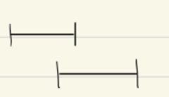
\[ \frac{n^4}{2^4} = \frac{n}{2} \cdot (\frac{n}{2})^3 = \sum_{i = \frac{n}{2}}^n (\frac{n}{2})^3 \leq \sum_{i = 1}^n i^3 = 1^3 + \ ... \ + (\frac{n}{2})^3 + \ ... \ + n^3 \]
Here we take only the n/2 term.
\[ \frac{n^4}{2^4} = \frac{n}{2} \cdot (\frac{n}{2})^3 = \sum_{i = \frac{n}{2}}^n (\frac{n}{2})^3 \leq \sum_{i = 1}^n i^3 = 1^3 + \ ... \ + (\frac{n}{2})^3 + \ ... \ + n^3 \]
Here we take only the n/2 term.
Current
Note has been deleted
Field-by-field Comparison
| Field | Before | After |
|---|---|---|
| Front | ||
| Back |
Note 78: ETH::1. Semester::A&D
Deck: ETH::1. Semester::A&D
Note Type: Horvath Classic
GUID:
deleted
Note Type: Horvath Classic
GUID:
H{hvq(0Rc-
Deleted Note
Front
Sei \(G\) ein ungerichteter, gewichteter und zusammenhängender Graph.
Nehmen Sie an, dass es eine eindeutige Kante mit Gewicht \(1\) gibt und, dass das Gewicht aller anderen Kanten strikt größer als \(1\) ist.
Nehmen Sie an, dass es eine eindeutige Kante mit Gewicht \(1\) gibt und, dass das Gewicht aller anderen Kanten strikt größer als \(1\) ist.
Dann enthält jeder minimale Spannbaum von \(G\) die Kante \(e\).
Back
Sei \(G\) ein ungerichteter, gewichteter und zusammenhängender Graph.
Nehmen Sie an, dass es eine eindeutige Kante mit Gewicht \(1\) gibt und, dass das Gewicht aller anderen Kanten strikt größer als \(1\) ist.
Nehmen Sie an, dass es eine eindeutige Kante mit Gewicht \(1\) gibt und, dass das Gewicht aller anderen Kanten strikt größer als \(1\) ist.
Dann enthält jeder minimale Spannbaum von \(G\) die Kante \(e\).
True
Wir wählen immer die Kante \(e\), weil sie die günstigste Art die ZHK's zu verbinden ist.
Siehe Cut Property.
Wir wählen immer die Kante \(e\), weil sie die günstigste Art die ZHK's zu verbinden ist.
Siehe Cut Property.
Current
Note has been deleted
Field-by-field Comparison
| Field | Before | After |
|---|---|---|
| Front | ||
| Back |
Note 79: ETH::1. Semester::A&D
Deck: ETH::1. Semester::A&D
Note Type: Horvath Classic
GUID:
deleted
Note Type: Horvath Classic
GUID:
I&{k}F8qaf
Deleted Note
Front
What edges cannot appear in a graph?
Back
What edges cannot appear in a graph?
- Self-loops (\(\{v, v\} \in V\))
- Multigraphs, i.e. same edge twice in the same graph
Current
Note has been deleted
Field-by-field Comparison
| Field | Before | After |
|---|---|---|
| Front | ||
| Back |
Note 80: ETH::1. Semester::A&D
Deck: ETH::1. Semester::A&D
Note Type: Horvath Cloze
GUID:
deleted
Note Type: Horvath Cloze
GUID:
IE=7&p8[(7
Deleted Note
Front
In an undirected graph, what is special about pre/post-ordering:
- back-edges = forward-edges
- cross edges are not possible
Back
In an undirected graph, what is special about pre/post-ordering:
- back-edges = forward-edges
- cross edges are not possible
Current
Note has been deleted
Field-by-field Comparison
| Field | Before | After |
|---|---|---|
| Text |
Note 81: ETH::1. Semester::A&D
Deck: ETH::1. Semester::A&D
Note Type: Horvath Cloze
GUID:
deleted
Note Type: Horvath Cloze
GUID:
IV81kgA3~6
Deleted Note
Front
Prim's Algorithm Invariants:
\(\forall v \not \in S, v \neq s\), \(d[v] = \) {{c1:: \(\min \{ w(u, v) \ | \ (u, v) \in E, u \in S \}\)(\(\infty\) if no such edge exists)}}.
\(\forall v \not \in S, v \neq s\), \(d[v] = \) {{c1:: \(\min \{ w(u, v) \ | \ (u, v) \in E, u \in S \}\)(\(\infty\) if no such edge exists)}}.
Back
Prim's Algorithm Invariants:
\(\forall v \not \in S, v \neq s\), \(d[v] = \) {{c1:: \(\min \{ w(u, v) \ | \ (u, v) \in E, u \in S \}\)(\(\infty\) if no such edge exists)}}.
\(\forall v \not \in S, v \neq s\), \(d[v] = \) {{c1:: \(\min \{ w(u, v) \ | \ (u, v) \in E, u \in S \}\)(\(\infty\) if no such edge exists)}}.
The 3rd invariant \[d[v] = \begin{cases} 0, & \text{if } v = s \text{ (the starting vertex)} \\ \min_{(u,v) \in E : u \in S} {w(u,v)}, & \text{if } v \in V \setminus S \text{ and } \exists (u,v) \in E \text{ with } u \in S \\ \infty, & \text{if } v \in V \setminus S \text{ and } \nexists (u,v) \in E \text{ with } u \in S \end{cases}\]ensures that d[v] always reflects the minimum cost to reach vertex v from the current MST.
We always want to add the vertex with the cheapest edge connecting it to the MST, thus this invariant has to hold in order for the algorithm to be correct.
Current
Note has been deleted
Field-by-field Comparison
| Field | Before | After |
|---|---|---|
| Text | ||
| Extra |
Note 82: ETH::1. Semester::A&D
Deck: ETH::1. Semester::A&D
Note Type: Horvath Cloze
GUID:
deleted
Note Type: Horvath Cloze
GUID:
IXC|=r,qdR
Deleted Note
Front
The distance \(d(u, v)\) in a directed graph is defined as shortest length of a walk from \(u\) to \(v\).
Back
The distance \(d(u, v)\) in a directed graph is defined as shortest length of a walk from \(u\) to \(v\).
Keep in mind in a weighted graph, this might mean the cheapest, which refers to cost not length.
Current
Note has been deleted
Field-by-field Comparison
| Field | Before | After |
|---|---|---|
| Text | ||
| Extra |
Note 83: ETH::1. Semester::A&D
Deck: ETH::1. Semester::A&D
Note Type: Horvath Classic
GUID:
deleted
Note Type: Horvath Classic
GUID:
Ip_w|jj[VT
Deleted Note
Front
How can we quickly check whether an Eulerian walk exists?
Back
How can we quickly check whether an Eulerian walk exists?
We can check the degrees of the vertices, an Eulerian walk exists only if at most 2 vertices have an odd degree
This is because if a vertex has an odd degree, it must either be the start point or the endpoint as otherwise we would not be able to leave from it
This is because if a vertex has an odd degree, it must either be the start point or the endpoint as otherwise we would not be able to leave from it
Current
Note has been deleted
Field-by-field Comparison
| Field | Before | After |
|---|---|---|
| Front | ||
| Back |
Note 84: ETH::1. Semester::A&D
Deck: ETH::1. Semester::A&D
Note Type: Horvath Cloze
GUID:
deleted
Note Type: Horvath Cloze
GUID:
J!K^!6M$e^
Deleted Note
Front
Differences between Subarray vs. Subsequence vs. Subset:
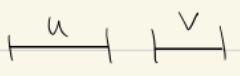
- Subarray: continous partition of the original
- Subsequence: non-continous partition
- Subset: any subset (order does not matter)
Back
Differences between Subarray vs. Subsequence vs. Subset:
- Subarray: continous partition of the original
- Subsequence: non-continous partition
- Subset: any subset (order does not matter)
Current
Note has been deleted
Field-by-field Comparison
| Field | Before | After |
|---|---|---|
| Text |
Note 85: ETH::1. Semester::A&D
Deck: ETH::1. Semester::A&D
Note Type: Horvath Cloze
GUID:
deleted
Note Type: Horvath Cloze
GUID:
J%Ue&}vC`>
Deleted Note
Front
In a directed graph, for the edge \(e = (u, v)\), \(u\) is the direct predecessor (Vorgänger) of \(v\) and \(v\) the direct successor (Nachfolger of \(u\).
Back
In a directed graph, for the edge \(e = (u, v)\), \(u\) is the direct predecessor (Vorgänger) of \(v\) and \(v\) the direct successor (Nachfolger of \(u\).
Current
Note has been deleted
Field-by-field Comparison
| Field | Before | After |
|---|---|---|
| Text |
Note 86: ETH::1. Semester::A&D
Deck: ETH::1. Semester::A&D
Note Type: Horvath Cloze
GUID:
deleted
Note Type: Horvath Cloze
GUID:
J5#2&7I#l3
Deleted Note
Front
A vertex with {{c1::\(\deg_{\text{out} }(v) = 0\)}} is called a sink (Senke).
Back
A vertex with {{c1::\(\deg_{\text{out} }(v) = 0\)}} is called a sink (Senke).
Current
Note has been deleted
Field-by-field Comparison
| Field | Before | After |
|---|---|---|
| Text |
Note 87: ETH::1. Semester::A&D
Deck: ETH::1. Semester::A&D
Note Type: Horvath Cloze
GUID:
deleted
Note Type: Horvath Cloze
GUID:
J5>uyKCn19
Deleted Note
Front
The ADT Dictionary implements the following methods:
- search(x, W) returns the position of the key x in memory
- insert(x, W) Insert the key x into W, as long as it’s not saved there yet
- delete(x, W) find and delete the key x from W
Back
The ADT Dictionary implements the following methods:
- search(x, W) returns the position of the key x in memory
- insert(x, W) Insert the key x into W, as long as it’s not saved there yet
- delete(x, W) find and delete the key x from W
Current
Note has been deleted
Field-by-field Comparison
| Field | Before | After |
|---|---|---|
| Text |
Note 88: ETH::1. Semester::A&D
Deck: ETH::1. Semester::A&D
Note Type: Horvath Cloze
GUID:
deleted
Note Type: Horvath Cloze
GUID:
Jm.C(wC@Lp
Deleted Note
Front
{{c1:: \(\sum_{i = 1}^{n} i^2\)::Sum}} \(=\) {{c2::\(\frac{n(n + 1)(2n + 1)}{6}\)}}
Back
{{c1:: \(\sum_{i = 1}^{n} i^2\)::Sum}} \(=\) {{c2::\(\frac{n(n + 1)(2n + 1)}{6}\)}}
Current
Note has been deleted
Field-by-field Comparison
| Field | Before | After |
|---|---|---|
| Text |
Note 89: ETH::1. Semester::A&D
Deck: ETH::1. Semester::A&D
Note Type: Horvath Cloze
GUID:
deleted
Note Type: Horvath Cloze
GUID:
Jm{y&aYo^p
Deleted Note
Front
For \(u, v \in V\) we say that \(u\) reaches \(v\) (erreicht) if there is a walk with endpoints \(u\) and \(v\) (or a path).
Back
For \(u, v \in V\) we say that \(u\) reaches \(v\) (erreicht) if there is a walk with endpoints \(u\) and \(v\) (or a path).
Reachability is an equivalence relation.
Current
Note has been deleted
Field-by-field Comparison
| Field | Before | After |
|---|---|---|
| Text | ||
| Extra |
Note 90: ETH::1. Semester::A&D
Deck: ETH::1. Semester::A&D
Note Type: Horvath Cloze
GUID:
deleted
Note Type: Horvath Cloze
GUID:
Jp{gN:I7yh
Deleted Note
Front
{{c1:: \(\sum_{i = 1}^{n} \log(i)\)::Sum}} \(=\) \(\log(n!)\)
Back
{{c1:: \(\sum_{i = 1}^{n} \log(i)\)::Sum}} \(=\) \(\log(n!)\)
Current
Note has been deleted
Field-by-field Comparison
| Field | Before | After |
|---|---|---|
| Text |
Note 91: ETH::1. Semester::A&D
Deck: ETH::1. Semester::A&D
Note Type: Horvath Classic
GUID:
deleted
Note Type: Horvath Classic
GUID:
K(FaD(&[!I
Deleted Note
Front
In an undirected graph, what does \(E\) contain?
Back
In an undirected graph, what does \(E\) contain?
\(E\) is the set of all edges, which are unordered pairs \(e = \{u, v\}\).
Current
Note has been deleted
Field-by-field Comparison
| Field | Before | After |
|---|---|---|
| Front | ||
| Back |
Note 92: ETH::1. Semester::A&D
Deck: ETH::1. Semester::A&D
Note Type: Horvath Cloze
GUID:
deleted
Note Type: Horvath Cloze
GUID:
KCjL6r:?jQ
Deleted Note
Front
A graph with more than \(n-1\) edges has a cycle if it is undirected.
Back
A graph with more than \(n-1\) edges has a cycle if it is undirected.
Current
Note has been deleted
Field-by-field Comparison
| Field | Before | After |
|---|---|---|
| Text |
Note 93: ETH::1. Semester::A&D
Deck: ETH::1. Semester::A&D
Note Type: Algorithms
GUID:
deleted
Note Type: Algorithms
GUID:
KD23pBO,?%
Deleted Note
Front
Back
Runtime of
Johnson
Runtime: {{c1::\( \mathcal{O}(|E| \cdot |V| + |V|^2 \cdot \log|V|)\)}}
Approach:
Uses:
?Current
Note has been deleted
Field-by-field Comparison
| Field | Before | After |
|---|---|---|
| Name |
Note 94: ETH::1. Semester::A&D
Deck: ETH::1. Semester::A&D
Note Type: Horvath Cloze
GUID:
deleted
Note Type: Horvath Cloze
GUID:
KgqO:Z_iT+
Deleted Note
Front
Choose a tight bound!
\(\sqrt n \leq O(n)\)
\(\sqrt n \leq O(n)\)
Back
Choose a tight bound!
\(\sqrt n \leq O(n)\)
\(\sqrt n \leq O(n)\)
Current
Note has been deleted
Field-by-field Comparison
| Field | Before | After |
|---|---|---|
| Text |
Note 95: ETH::1. Semester::A&D
Deck: ETH::1. Semester::A&D
Note Type: Image Occlusion-73a2c
GUID:
deleted
Note Type: Image Occlusion-73a2c
GUID:
KoR^|Dl^:[
Deleted Note
Front

Back
Current
Note has been deleted
Field-by-field Comparison
| Field | Before | After |
|---|---|---|
| Occlusion | ||
| Image |
Note 96: ETH::1. Semester::A&D
Deck: ETH::1. Semester::A&D
Note Type: Horvath Classic
GUID:
deleted
Note Type: Horvath Classic
GUID:
L#@+crYi2-
Deleted Note
Front
Bipartite Test with BFS:
Back
Bipartite Test with BFS:
We substitute bipartite for two-colourable.
While traversing the tree, in each layer, we colour all vertices with the same. If we then encounter a vertex with the same colour during traversal, it's not two-colourable.
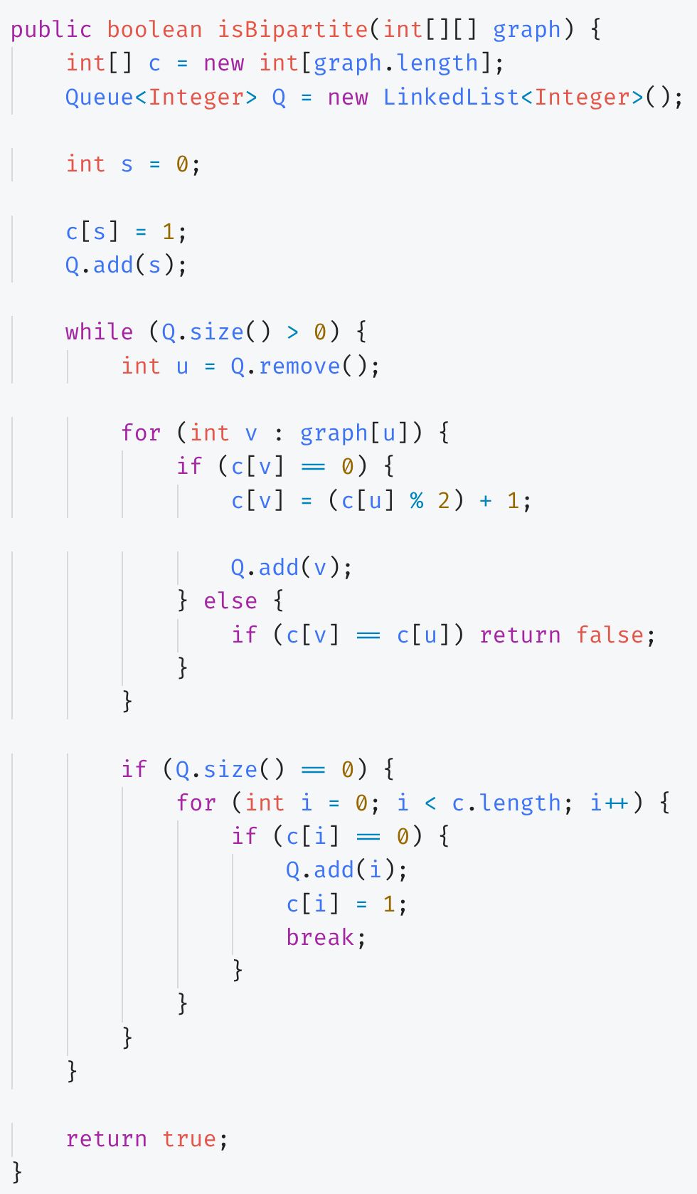
While traversing the tree, in each layer, we colour all vertices with the same. If we then encounter a vertex with the same colour during traversal, it's not two-colourable.
Current
Note has been deleted
Field-by-field Comparison
| Field | Before | After |
|---|---|---|
| Front | ||
| Back |
Note 97: ETH::1. Semester::A&D
Deck: ETH::1. Semester::A&D
Note Type: Horvath Classic
GUID:
deleted
Note Type: Horvath Classic
GUID:
L4[cTT%fZ]
Deleted Note
Front
Provide the outline of an induction proof.
Back
Provide the outline of an induction proof.
We want to prove that ... for \(n \geq 5\)
Base Case: Let \(n = 5\) .... So the property holds for \(n = 5\).
Induction Hypothesis: We assume the property is true for some \(k \geq 5\)
Induction Step: We must show that the property holds for \(k + 1\).
By the principle of mathematical induction ... is true for all \(n \geq 5\).
Base Case: Let \(n = 5\) .... So the property holds for \(n = 5\).
Induction Hypothesis: We assume the property is true for some \(k \geq 5\)
Induction Step: We must show that the property holds for \(k + 1\).
By the principle of mathematical induction ... is true for all \(n \geq 5\).
Current
Note has been deleted
Field-by-field Comparison
| Field | Before | After |
|---|---|---|
| Front | ||
| Back |
Note 98: ETH::1. Semester::A&D
Deck: ETH::1. Semester::A&D
Note Type: Horvath Cloze
GUID:
deleted
Note Type: Horvath Cloze
GUID:
LGV&:!
Deleted Note
Front
Prim's Algorithm requires an undirected, connected, weighted Graph.
Back
Prim's Algorithm requires an undirected, connected, weighted Graph.
Current
Note has been deleted
Field-by-field Comparison
| Field | Before | After |
|---|---|---|
| Text |
Note 99: ETH::1. Semester::A&D
Deck: ETH::1. Semester::A&D
Note Type: Algorithms
GUID:
deleted
Note Type: Algorithms
GUID:
L`3Iw:nx:Z
Deleted Note
Front
Runtime of Subset Sum (Teilsummenproblem)?
Back
Runtime of Subset Sum (Teilsummenproblem)?
\(\Theta(n \cdot b)\) (Pseudo-Polynomial)
Current
Note has been deleted
Field-by-field Comparison
| Field | Before | After |
|---|---|---|
| Name | ||
| Runtime | ||
| Requirements |
Note 100: ETH::1. Semester::A&D
Deck: ETH::1. Semester::A&D
Note Type: Horvath Cloze
GUID:
deleted
Note Type: Horvath Cloze
GUID:
Ld,vXkta~C
Deleted Note
Front
The ADT priorityQueue has the following operations:
- insert: insert with priority p
- extractMax: removes and returns element with highest priority.
Back
The ADT priorityQueue has the following operations:
- insert: insert with priority p
- extractMax: removes and returns element with highest priority.
Current
Note has been deleted
Field-by-field Comparison
| Field | Before | After |
|---|---|---|
| Text |
Note 101: ETH::1. Semester::A&D
Deck: ETH::1. Semester::A&D
Note Type: Algorithms
GUID:
deleted
Note Type: Algorithms
GUID:
LqP`8lU$&o
Deleted Note
Front
Runtime of Insertion Sort?
Back
Runtime of Insertion Sort?
Best Case: \(O(n \log n)\)
Worst Case: \(O(n^2)\)
This insertion is not in constant time! We have to swap with each previous element!
Current
Note has been deleted
Field-by-field Comparison
| Field | Before | After |
|---|---|---|
| Name | ||
| Runtime | ||
| Approach | ||
| Pseudocode | ||
| Extra Info | ||
| Invariant | ||
| Worst Case Scenario | ||
| Attributes |
Note 102: ETH::1. Semester::A&D
Deck: ETH::1. Semester::A&D
Note Type: Algorithms
GUID:
deleted
Note Type: Algorithms
GUID:
L~wgr~ELJV
Deleted Note
Front
Runtime of Knapsack Problem (Rucksackproblem)?
Back
Runtime of Knapsack Problem (Rucksackproblem)?
\(\Theta(n\cdot W)\) or \(\Theta(n \cdot P)\) (Pseudopolynomial)
Current
Note has been deleted
Field-by-field Comparison
| Field | Before | After |
|---|---|---|
| Name | ||
| Runtime | ||
| Approach | ||
| Pseudocode |
Note 103: ETH::1. Semester::A&D
Deck: ETH::1. Semester::A&D
Note Type: Horvath Cloze
GUID:
deleted
Note Type: Horvath Cloze
GUID:
M,7!v0F$PQ
Deleted Note
Front
A connected component of \(G\) is a equivalence class of the relation defined as follows: \(u = v\) if \(u\) reaches \(v\).
Back
A connected component of \(G\) is a equivalence class of the relation defined as follows: \(u = v\) if \(u\) reaches \(v\).
Current
Note has been deleted
Field-by-field Comparison
| Field | Before | After |
|---|---|---|
| Text |
Note 104: ETH::1. Semester::A&D
Deck: ETH::1. Semester::A&D
Note Type: Horvath Cloze
GUID:
deleted
Note Type: Horvath Cloze
GUID:
M,?u9cw(S%
Deleted Note
Front
{{c1:: \(\sum_{i = 1}^{n} i\log(i)\)::Sum}} \(\leq\) \(O(n \log(n))\)
Back
{{c1:: \(\sum_{i = 1}^{n} i\log(i)\)::Sum}} \(\leq\) \(O(n \log(n))\)
Current
Note has been deleted
Field-by-field Comparison
| Field | Before | After |
|---|---|---|
| Text |
Note 105: ETH::1. Semester::A&D
Deck: ETH::1. Semester::A&D
Note Type: Horvath Cloze
GUID:
deleted
Note Type: Horvath Cloze
GUID:
M11/nZaHIu
Deleted Note
Front
| Search | Insertion | Deletion | |
| Non-sorted array | \(O(n)\) | \(O(1)\) | \(O(n)\) |
| Sorted array | \(O(\log n)\) | \(O(n)\) | \(O(n)\) |
| Doubly linked list | \(O(n)\) | \(O(1)\) | \(O(1)\) |
Back
| Search | Insertion | Deletion | |
| Non-sorted array | \(O(n)\) | \(O(1)\) | \(O(n)\) |
| Sorted array | \(O(\log n)\) | \(O(n)\) | \(O(n)\) |
| Doubly linked list | \(O(n)\) | \(O(1)\) | \(O(1)\) |
Current
Note has been deleted
Field-by-field Comparison
| Field | Before | After |
|---|---|---|
| Text |
Note 106: ETH::1. Semester::A&D
Deck: ETH::1. Semester::A&D
Note Type: Horvath Classic
GUID:
deleted
Note Type: Horvath Classic
GUID:
M?qP8s.,s4
Deleted Note
Front
How can we represent a graph?
Back
How can we represent a graph?
1. Adjacency matrix
2. Adjacency lists
2. Adjacency lists
Current
Note has been deleted
Field-by-field Comparison
| Field | Before | After |
|---|---|---|
| Front | ||
| Back |
Note 107: ETH::1. Semester::A&D
Deck: ETH::1. Semester::A&D
Note Type: Horvath Classic
GUID:
deleted
Note Type: Horvath Classic
GUID:
MFFs/r0>#}
Deleted Note
Front
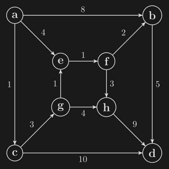
Can (g, h) ever be in an MST? Prove it:
Back
Can (g, h) ever be in an MST? Prove it:
No, because it's the heaviest edge in the cycle.
If there was an MST containing it, we could remove it and replace it by another edge in the cycle.
Then we preserve the tree property yet it's weight is strictly lower.
If there was an MST containing it, we could remove it and replace it by another edge in the cycle.
Then we preserve the tree property yet it's weight is strictly lower.
Current
Note has been deleted
Field-by-field Comparison
| Field | Before | After |
|---|---|---|
| Front | ||
| Back |
Note 108: ETH::1. Semester::A&D
Deck: ETH::1. Semester::A&D
Note Type: Horvath Classic
GUID:
deleted
Note Type: Horvath Classic
GUID:
M^6zMs=8ah
Deleted Note
Front
What is the sum of all natural numbers between 1 and \(n\)?
Back
What is the sum of all natural numbers between 1 and \(n\)?
\(= \frac{n(n+1)}{2}\)
Current
Note has been deleted
Field-by-field Comparison
| Field | Before | After |
|---|---|---|
| Front | ||
| Back |
Note 109: ETH::1. Semester::A&D
Deck: ETH::1. Semester::A&D
Note Type: Horvath Cloze
GUID:
deleted
Note Type: Horvath Cloze
GUID:
Mv|.Tnx#vx
Deleted Note
Front
A graph with distinct edge weights has one single unique MST.
Back
A graph with distinct edge weights has one single unique MST.
There is one unique safe-edge.
Current
Note has been deleted
Field-by-field Comparison
| Field | Before | After |
|---|---|---|
| Text | ||
| Extra |
Note 110: ETH::1. Semester::A&D
Deck: ETH::1. Semester::A&D
Note Type: Horvath Cloze
GUID:
deleted
Note Type: Horvath Cloze
GUID:
N9}LnE{]~X
Deleted Note
Front
In an edge \(e = \{u, v\}\), we call \(u\) adjacent (adjazent oder benachbart) to \(v\) (and the other way around) and \(e\) incident (inzident oder anliegend) to \(u, v\).
Back
In an edge \(e = \{u, v\}\), we call \(u\) adjacent (adjazent oder benachbart) to \(v\) (and the other way around) and \(e\) incident (inzident oder anliegend) to \(u, v\).
Current
Note has been deleted
Field-by-field Comparison
| Field | Before | After |
|---|---|---|
| Text |
Note 111: ETH::1. Semester::A&D
Deck: ETH::1. Semester::A&D
Note Type: Horvath Classic
GUID:
deleted
Note Type: Horvath Classic
GUID:
N@-]h|e+xG
Deleted Note
Front
Runtime: Operations in an Adjacency List:
Back
Runtime: Operations in an Adjacency List:
1. Check if \(uv \in E \): \(O(1 + \min\{\text{deg}(u), \text{deg}(v) \})\) (we have to check the smaller of the two adjacency lists
2. Vertex \(u\), find all adjacent vertices: \(O(1+\text{deg}(u) )\)
2. Vertex \(u\), find all adjacent vertices: \(O(1+\text{deg}(u) )\)
Current
Note has been deleted
Field-by-field Comparison
| Field | Before | After |
|---|---|---|
| Front | ||
| Back |
Note 112: ETH::1. Semester::A&D
Deck: ETH::1. Semester::A&D
Note Type: Algorithms
GUID:
deleted
Note Type: Algorithms
GUID:
NAHrkHd^ik
Deleted Note
Front
Runtime of Merge Sort?
Back
Runtime of Merge Sort?
Best Case: \(O(n \log n)\)
Worst Case: \(O(n \log n)\)
Worst Case: \(O(n \log n)\)
Current
Note has been deleted
Field-by-field Comparison
| Field | Before | After |
|---|---|---|
| Name | ||
| Runtime | ||
| Approach | ||
| Pseudocode | ||
| Invariant | ||
| Worst Case Scenario | ||
| Attributes |
Note 113: ETH::1. Semester::A&D
Deck: ETH::1. Semester::A&D
Note Type: Horvath Cloze
GUID:
deleted
Note Type: Horvath Cloze
GUID:
NDIo0EK5KX
Deleted Note
Front
If \(T(n) \geq aT(n/ 2) + Cn^b\), then the O-Notation gives \(T(n) \geq \) \(\Omega(...)\).
Back
If \(T(n) \geq aT(n/ 2) + Cn^b\), then the O-Notation gives \(T(n) \geq \) \(\Omega(...)\).
Current
Note has been deleted
Field-by-field Comparison
| Field | Before | After |
|---|---|---|
| Text |
Note 114: ETH::1. Semester::A&D
Deck: ETH::1. Semester::A&D
Note Type: Horvath Cloze
GUID:
deleted
Note Type: Horvath Cloze
GUID:
NGdgt3D+pd
Deleted Note
Front
We can ignore the base of a logarithm only if it's not in the exponent.
Back
We can ignore the base of a logarithm only if it's not in the exponent.
\(e^{\log_2 n} \neq \Theta(e^{\log_3 n})\) as \(e^{\log_2 n - \log_3 n} = e^{\ln n (\frac{1}{\ln(2)} - \frac{1}{\ln(3)})}\) goes to \(\infty\)
Current
Note has been deleted
Field-by-field Comparison
| Field | Before | After |
|---|---|---|
| Text | ||
| Extra |
Note 115: ETH::1. Semester::A&D
Deck: ETH::1. Semester::A&D
Note Type: Horvath Classic
GUID:
deleted
Note Type: Horvath Classic
GUID:
NR^|^~o+xa
Deleted Note
Front
How do we get a topological sorting from DFS?
Back
How do we get a topological sorting from DFS?
Reversed post order
Current
Note has been deleted
Field-by-field Comparison
| Field | Before | After |
|---|---|---|
| Front | ||
| Back |
Note 116: ETH::1. Semester::A&D
Deck: ETH::1. Semester::A&D
Note Type: Horvath Cloze
GUID:
deleted
Note Type: Horvath Cloze
GUID:
NU;6ob<^n3
Deleted Note
Front
{{c1:: \(\sum_{i = 1}^{n} \sum_{k = 1}^{\textbf{i} } 1\)::Sum}} \(=\) {{c2:: \(\sum_{i = 1}^n i = \frac{n(n + 1)}{2}\)}}
Back
{{c1:: \(\sum_{i = 1}^{n} \sum_{k = 1}^{\textbf{i} } 1\)::Sum}} \(=\) {{c2:: \(\sum_{i = 1}^n i = \frac{n(n + 1)}{2}\)}}
inner loop depends on outer
Current
Note has been deleted
Field-by-field Comparison
| Field | Before | After |
|---|---|---|
| Text | ||
| Extra |
Note 117: ETH::1. Semester::A&D
Deck: ETH::1. Semester::A&D
Note Type: Horvath Classic
GUID:
deleted
Note Type: Horvath Classic
GUID:
Nl}2-%ar31
Deleted Note
Front
What is a maxHeap?
Back
What is a maxHeap?
A datastructure that stores the values in a tree form, with the largest element always as the root.
Current
Note has been deleted
Field-by-field Comparison
| Field | Before | After |
|---|---|---|
| Front | ||
| Back |
Note 118: ETH::1. Semester::A&D
Deck: ETH::1. Semester::A&D
Note Type: Horvath Cloze
GUID:
deleted
Note Type: Horvath Cloze
GUID:
O%OM.97hp$
Deleted Note
Front
\(\exists\) back edge \(\Longleftrightarrow\)\(\exists\) directed closed walk
Back
\(\exists\) back edge \(\Longleftrightarrow\)\(\exists\) directed closed walk
Current
Note has been deleted
Field-by-field Comparison
| Field | Before | After |
|---|---|---|
| Text |
Note 119: ETH::1. Semester::A&D
Deck: ETH::1. Semester::A&D
Note Type: Horvath Cloze
GUID:
deleted
Note Type: Horvath Cloze
GUID:
O5ty{6nA_*
Deleted Note
Front
The degree (Knotengrad) \(\deg(v)\) of a vertex \(v\) is the number of edges that are incident to \(v\).
Back
The degree (Knotengrad) \(\deg(v)\) of a vertex \(v\) is the number of edges that are incident to \(v\).
Current
Note has been deleted
Field-by-field Comparison
| Field | Before | After |
|---|---|---|
| Text |
Note 120: ETH::1. Semester::A&D
Deck: ETH::1. Semester::A&D
Note Type: Horvath Classic
GUID:
deleted
Note Type: Horvath Classic
GUID:
O>N2*/v~`q
Deleted Note
Front
If a vertex has degree 0, what do we call it?
Back
If a vertex has degree 0, what do we call it?
It is an isolated vertex.
Current
Note has been deleted
Field-by-field Comparison
| Field | Before | After |
|---|---|---|
| Front | ||
| Back |
Note 121: ETH::1. Semester::A&D
Deck: ETH::1. Semester::A&D
Note Type: Horvath Cloze
GUID:
deleted
Note Type: Horvath Cloze
GUID:
OGBoPi1aY*
Deleted Note
Front
The ADTs stack and queue behave similarly to a list, but with more constrained operations that allow more efficient computation.
Back
The ADTs stack and queue behave similarly to a list, but with more constrained operations that allow more efficient computation.
Current
Note has been deleted
Field-by-field Comparison
| Field | Before | After |
|---|---|---|
| Text |
Note 122: ETH::1. Semester::A&D
Deck: ETH::1. Semester::A&D
Note Type: Horvath Classic
GUID:
deleted
Note Type: Horvath Classic
GUID:
OIsr/vHbhR
Deleted Note
Front
What do we have to pay attention to in the I.H. and the I.S. in an induction proof?
Back
What do we have to pay attention to in the I.H. and the I.S. in an induction proof?
We should change the variable name from \(n\) to \(k\) (for example) as not to confuse it.
Current
Note has been deleted
Field-by-field Comparison
| Field | Before | After |
|---|---|---|
| Front | ||
| Back |
Note 123: ETH::1. Semester::A&D
Deck: ETH::1. Semester::A&D
Note Type: Horvath Reverso
GUID:
deleted
Note Type: Horvath Reverso
GUID:
OW(TL-EP^P
Deleted Note
Front
Cycle
Back
Cycle
Kreis
Current
Note has been deleted
Field-by-field Comparison
| Field | Before | After |
|---|---|---|
| Front | ||
| Back |
Note 124: ETH::1. Semester::A&D
Deck: ETH::1. Semester::A&D
Note Type: Horvath Cloze
GUID:
deleted
Note Type: Horvath Cloze
GUID:
OY@2Ay+>4p
Deleted Note
Front
2-3 Tree: Deletion steps:
- Search for the correct node under which the key is inserted: \(O(\log_2 n)\)
- Remove the leaf with the value and one separator
- Rebalance (if necessary, i.e. now 1 key)
Back
2-3 Tree: Deletion steps:
- Search for the correct node under which the key is inserted: \(O(\log_2 n)\)
- Remove the leaf with the value and one separator
- Rebalance (if necessary, i.e. now 1 key)
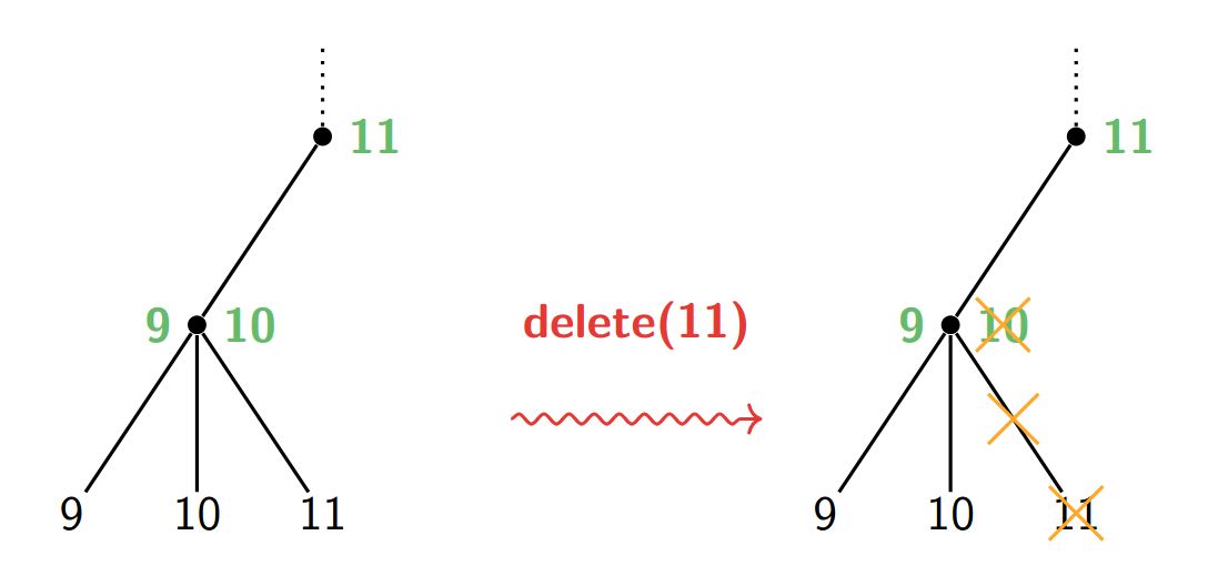
Current
Note has been deleted
Field-by-field Comparison
| Field | Before | After |
|---|---|---|
| Text | ||
| Extra |
Note 125: ETH::1. Semester::A&D
Deck: ETH::1. Semester::A&D
Note Type: Horvath Classic
GUID:
deleted
Note Type: Horvath Classic
GUID:
OeCuLqI!|5
Deleted Note
Front
Extra memory requirements of Heapsort?
Back
Extra memory requirements of Heapsort?
\(O(1)\) as we simply arrange the array into a heap.
Current
Note has been deleted
Field-by-field Comparison
| Field | Before | After |
|---|---|---|
| Front | ||
| Back |
Note 126: ETH::1. Semester::A&D
Deck: ETH::1. Semester::A&D
Note Type: Horvath Classic
GUID:
deleted
Note Type: Horvath Classic
GUID:
Otnyr;#TD1
Deleted Note
Front
Simplify \(\frac{a^{kn}}{b^{k'n}} =\)
Back
Simplify \(\frac{a^{kn}}{b^{k'n}} =\)
\(\frac{e^{\ln(a^{kn})}}{e^{\ln(b^{k'n})}} = e^{kn \cdot \ln(a) - k'n \cdot ln(b)}\)
Current
Note has been deleted
Field-by-field Comparison
| Field | Before | After |
|---|---|---|
| Front | ||
| Back |
Note 127: ETH::1. Semester::A&D
Deck: ETH::1. Semester::A&D
Note Type: Horvath Classic
GUID:
deleted
Note Type: Horvath Classic
GUID:
O||9vPX+Y`
Deleted Note
Front
When \(f = \Theta(g)\), this means?
Back
When \(f = \Theta(g)\), this means?
\(\exists C_1,C_2 \ge 0 \quad \forall n \in \mathbb{N}\) \(C_1 \cdot g(n) \leq f(n) \leq C_2 \cdot g(n)\)
\(f\) grows asymptotically the same as \(g\).
\(f\) grows asymptotically the same as \(g\).
Current
Note has been deleted
Field-by-field Comparison
| Field | Before | After |
|---|---|---|
| Front | ||
| Back |
Note 128: ETH::1. Semester::A&D
Deck: ETH::1. Semester::A&D
Note Type: Horvath Cloze
GUID:
deleted
Note Type: Horvath Cloze
GUID:
P<,uu+Hu
Deleted Note
Front
The shortest walk in a directed, weighted graph is always a path.
Back
The shortest walk in a directed, weighted graph is always a path.
If it's a walk, we can remove all edges between the first occurence of the repeated vertex and the last occurence.
Current
Note has been deleted
Field-by-field Comparison
| Field | Before | After |
|---|---|---|
| Text | ||
| Extra |
Note 129: ETH::1. Semester::A&D
Deck: ETH::1. Semester::A&D
Note Type: Horvath Cloze
GUID:
deleted
Note Type: Horvath Cloze
GUID:
P
Deleted Note
Front
A vertex in a connected graph is a cut vertex if the subgraph obtained after removing it and all it's incident edges is disconnected.
Back
A vertex in a connected graph is a cut vertex if the subgraph obtained after removing it and all it's incident edges is disconnected.
Current
Note has been deleted
Field-by-field Comparison
| Field | Before | After |
|---|---|---|
| Text |
Note 130: ETH::1. Semester::A&D
Deck: ETH::1. Semester::A&D
Note Type: Horvath Classic
GUID:
deleted
Note Type: Horvath Classic
GUID:
PF|EmWOMd:
Deleted Note
Front
Cost of a walk in a weighted graph \(G = (V, E, c)\)?
Back
Cost of a walk in a weighted graph \(G = (V, E, c)\)?
Sum of the weight of it's edges: \(\sum_{i = 0}^{l - 1} c(v_i, v_{i+1})\)
Current
Note has been deleted
Field-by-field Comparison
| Field | Before | After |
|---|---|---|
| Front | ||
| Back |
Note 131: ETH::1. Semester::A&D
Deck: ETH::1. Semester::A&D
Note Type: Horvath Classic
GUID:
deleted
Note Type: Horvath Classic
GUID:
PU(5RRppkP
Deleted Note
Front
When can the condition \(n = 2^k\) be dropped in the Master Theorem?
Back
When can the condition \(n = 2^k\) be dropped in the Master Theorem?
When the function \(T\) is increasing (monotonically non-decreasing).
Current
Note has been deleted
Field-by-field Comparison
| Field | Before | After |
|---|---|---|
| Front | ||
| Back |
Note 132: ETH::1. Semester::A&D
Deck: ETH::1. Semester::A&D
Note Type: Horvath Cloze
GUID:
deleted
Note Type: Horvath Cloze
GUID:
Pf|C9|^n[w
Deleted Note
Front
In a singly and doubly linked list, the operation:
- Insert is \(\Theta(1)\) as we know the memory address of the final element in the list and just have to set the null pointer to the new keys address. Without this pointer it's \(\Theta(l)\).
- Get is \(\Theta(i)\) very slow as we need to traverse the entire list up to i
- insertAfter is \(O(1)\) if we get the memory address of the element to insert after.
- delete is:
SLL: \(\Theta(l)\) as we need to find the previous element and change it's pointer.
DLL: \(O(1)\) we know the address of the previous element and then just edit it's pointer.
Back
In a singly and doubly linked list, the operation:
- Insert is \(\Theta(1)\) as we know the memory address of the final element in the list and just have to set the null pointer to the new keys address. Without this pointer it's \(\Theta(l)\).
- Get is \(\Theta(i)\) very slow as we need to traverse the entire list up to i
- insertAfter is \(O(1)\) if we get the memory address of the element to insert after.
- delete is:
SLL: \(\Theta(l)\) as we need to find the previous element and change it's pointer.
DLL: \(O(1)\) we know the address of the previous element and then just edit it's pointer.
Current
Note has been deleted
Field-by-field Comparison
| Field | Before | After |
|---|---|---|
| Text |
Note 133: ETH::1. Semester::A&D
Deck: ETH::1. Semester::A&D
Note Type: Horvath Cloze
GUID:
deleted
Note Type: Horvath Cloze
GUID:
PhZTjS+XL8
Deleted Note
Front
If \(\frac{f(n)}{g(n)}\) tends to \(\infty+\), then \(f \nleq O(g)\) and \(g \leq O(f)\).
Back
If \(\frac{f(n)}{g(n)}\) tends to \(\infty+\), then \(f \nleq O(g)\) and \(g \leq O(f)\).
\(f \geq \Omega(g)\) but \(f \neq \Theta(g)\)
Current
Note has been deleted
Field-by-field Comparison
| Field | Before | After |
|---|---|---|
| Text | ||
| Extra |
Note 134: ETH::1. Semester::A&D
Deck: ETH::1. Semester::A&D
Note Type: Horvath Cloze
GUID:
deleted
Note Type: Horvath Cloze
GUID:
PvmYSo9Bj_
Deleted Note
Front
In the edge \(e = (u, v)\), we call \(u\) the start vertex and \(v\) the end vertex.
Back
In the edge \(e = (u, v)\), we call \(u\) the start vertex and \(v\) the end vertex.
Current
Note has been deleted
Field-by-field Comparison
| Field | Before | After |
|---|---|---|
| Text |
Note 135: ETH::1. Semester::A&D
Deck: ETH::1. Semester::A&D
Note Type: Horvath Cloze
GUID:
deleted
Note Type: Horvath Cloze
GUID:
Q3:!A9V`D,
Deleted Note
Front
Steps of giving a DP solution:
- Define the DP table (dimensions, index, range; meaning of entry): ex: DP[1..n+1][1..k+1]
- Computation of entries (Base case, recursive formula, pay attention to bounds!)
- Order of calculation (what depends on what entries, what variable incremented first)
- Extracting the solution
- Runtime
Back
Steps of giving a DP solution:
- Define the DP table (dimensions, index, range; meaning of entry): ex: DP[1..n+1][1..k+1]
- Computation of entries (Base case, recursive formula, pay attention to bounds!)
- Order of calculation (what depends on what entries, what variable incremented first)
- Extracting the solution
- Runtime
SMIROST (Size, Meaning, Initialisation, Recursive Relation, Order, Solution, Time)


Smiling Monkey In Red Overall Steals Tacos
Smiling Monkey In Red Overall Steals Tacos
Current
Note has been deleted
Field-by-field Comparison
| Field | Before | After |
|---|---|---|
| Text | ||
| Extra |
Note 136: ETH::1. Semester::A&D
Deck: ETH::1. Semester::A&D
Note Type: Horvath Cloze
GUID:
deleted
Note Type: Horvath Cloze
GUID:
QA~(,/7jXV
Deleted Note
Front
Choose a tight bound!
\(O(k^n) \leq O(n!)\)
\(O(k^n) \leq O(n!)\)
Back
Choose a tight bound!
\(O(k^n) \leq O(n!)\)
\(O(k^n) \leq O(n!)\)
Current
Note has been deleted
Field-by-field Comparison
| Field | Before | After |
|---|---|---|
| Text |
Note 137: ETH::1. Semester::A&D
Deck: ETH::1. Semester::A&D
Note Type: Horvath Classic
GUID:
deleted
Note Type: Horvath Classic
GUID:
QBdl=YAmG|
Deleted Note
Front
How can we check for cycles via DFS?
Back
How can we check for cycles via DFS?
During the recursive call, if we find an adjacent vertex without a post-number, there's a back-edge (\(\implies\)the recursive call for that edge is still active...).
Current
Note has been deleted
Field-by-field Comparison
| Field | Before | After |
|---|---|---|
| Front | ||
| Back |
Note 138: ETH::1. Semester::A&D
Deck: ETH::1. Semester::A&D
Note Type: Image Occlusion-73a2c
GUID:
deleted
Note Type: Image Occlusion-73a2c
GUID:
QGU[QMk!u8
Deleted Note
Front
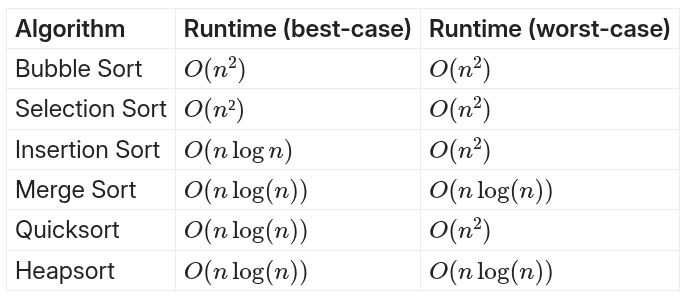
Back
Current
Note has been deleted
Field-by-field Comparison
| Field | Before | After |
|---|---|---|
| Occlusion | ||
| Image |
Note 139: ETH::1. Semester::A&D
Deck: ETH::1. Semester::A&D
Note Type: Horvath Cloze
GUID:
deleted
Note Type: Horvath Cloze
GUID:
QJ{Y%?s>+w
Deleted Note
Front
When writing a recursion which accesses an index that could go out of bounds, make sure to return a neutral value instead of crashing.
Back
When writing a recursion which accesses an index that could go out of bounds, make sure to return a neutral value instead of crashing.
Example: Subset Sum
Recursion: \(DP[i][B] = DP[i-1][B] \lor DP[i-1][B - b_i]\)
The term \(B - b_i\) can become negative. Instead of accessing an invalid index, return "false" (the neutral element for OR), since you can't achieve a negative sum.
Recursion: \(DP[i][B] = DP[i-1][B] \lor DP[i-1][B - b_i]\)
The term \(B - b_i\) can become negative. Instead of accessing an invalid index, return "false" (the neutral element for OR), since you can't achieve a negative sum.
Current
Note has been deleted
Field-by-field Comparison
| Field | Before | After |
|---|---|---|
| Text | ||
| Extra |
Note 140: ETH::1. Semester::A&D
Deck: ETH::1. Semester::A&D
Note Type: Horvath Classic
GUID:
deleted
Note Type: Horvath Classic
GUID:
Qv/bX3RU0v
Deleted Note
Front
How does the number of ZHK's change in Boruvka's for each round?
Back
How does the number of ZHK's change in Boruvka's for each round?
The number of components halves in each round, thus \(\log |V|\) iterations worst case.
Current
Note has been deleted
Field-by-field Comparison
| Field | Before | After |
|---|---|---|
| Front | ||
| Back |
Note 141: ETH::1. Semester::A&D
Deck: ETH::1. Semester::A&D
Note Type: Horvath Classic
GUID:
deleted
Note Type: Horvath Classic
GUID:
Q|AEYAPg!l
Deleted Note
Front
What is a sufficient condition to show that \(f \geq \Omega(g)\)?
Back
What is a sufficient condition to show that \(f \geq \Omega(g)\)?
Let \(N\) be an infinite subset of \(\mathbb{N}\) and \(f: N \rightarrow \mathbb{R}^+\) and \(g: N \rightarrow \mathbb{R}^+\)
then if \(\lim_{n\rightarrow \infty} \frac{f(n)}{g(n)} = \infty\), \(f \geq \Omega(g)\) but \(f \neq \Theta(g)\)
then if \(\lim_{n\rightarrow \infty} \frac{f(n)}{g(n)} = \infty\), \(f \geq \Omega(g)\) but \(f \neq \Theta(g)\)
Current
Note has been deleted
Field-by-field Comparison
| Field | Before | After |
|---|---|---|
| Front | ||
| Back |
Note 142: ETH::1. Semester::A&D
Deck: ETH::1. Semester::A&D
Note Type: Horvath Classic
GUID:
deleted
Note Type: Horvath Classic
GUID:
Q}a3<1,J]C
Deleted Note
Front
2-3 Tree: We deleted a node and now it's sibling is an only child. What happens if it's neighbor has 2 keys?
Back
2-3 Tree: We deleted a node and now it's sibling is an only child. What happens if it's neighbor has 2 keys?
- The nodes \(u\) and \(v\) are merged to form one new node with 3 children.
- The separator from the parent node is pulled down to be the new \(s_2\).
If root has 1 child -> root replaced by child.
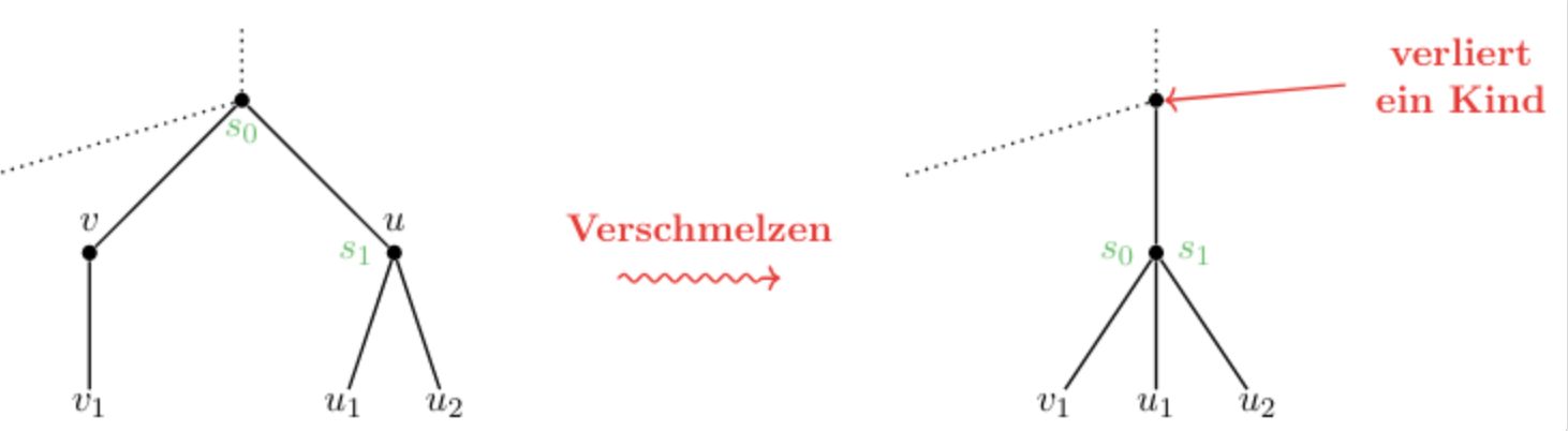
Current
Note has been deleted
Field-by-field Comparison
| Field | Before | After |
|---|---|---|
| Front | ||
| Back |
Note 143: ETH::1. Semester::A&D
Deck: ETH::1. Semester::A&D
Note Type: Horvath Cloze
GUID:
deleted
Note Type: Horvath Cloze
GUID:
R<,pyG}zC
Deleted Note
Front
Choose a tight bound!
\(O(\log(n))\leq O(n)\)
\(O(\log(n))\leq O(n)\)
Back
Choose a tight bound!
\(O(\log(n))\leq O(n)\)
\(O(\log(n))\leq O(n)\)
Current
Note has been deleted
Field-by-field Comparison
| Field | Before | After |
|---|---|---|
| Text |
Note 144: ETH::1. Semester::A&D
Deck: ETH::1. Semester::A&D
Note Type: Algorithms
GUID:
deleted
Note Type: Algorithms
GUID:
T?I`@dy&K
Deleted Note
Front
Runtime of Kruskal's Algorithm?
Back
Runtime of Kruskal's Algorithm?
\(O(|E| \log |E| + |V| \log |V|)\)
Outer loop: Iterate \(|E|\) times at most:
Inner loop: find and union take \(O(\log |V|)\) per call amortised, thus \(O(|V| \log |V|)\) total.
This requires the Union Find datastructure.
Outer loop: Iterate \(|E|\) times at most:
Inner loop: find and union take \(O(\log |V|)\) per call amortised, thus \(O(|V| \log |V|)\) total.
This requires the Union Find datastructure.
Current
Note has been deleted
Field-by-field Comparison
| Field | Before | After |
|---|---|---|
| Name | ||
| Runtime | ||
| Requirements | ||
| Approach | ||
| Pseudocode | ||
| Use Case | ||
| Extra Info |
Note 145: ETH::1. Semester::A&D
Deck: ETH::1. Semester::A&D
Note Type: Horvath Cloze
GUID:
deleted
Note Type: Horvath Cloze
GUID:
bD%.s|4?hI
Deleted Note
Front
Pre-/Post-Ordering Classification for an edge \((u, v)\):
\(\text{pre}(u) < \text{pre}(v) < \text{post}(v) < \text{post}(u)\): tree edge, as \(v\) is a descendant of \(u\)
\(\text{pre}(u) < \text{pre}(v) < \text{post}(v) < \text{post}(u)\): tree edge, as \(v\) is a descendant of \(u\)
Back
Pre-/Post-Ordering Classification for an edge \((u, v)\):
\(\text{pre}(u) < \text{pre}(v) < \text{post}(v) < \text{post}(u)\): tree edge, as \(v\) is a descendant of \(u\)
\(\text{pre}(u) < \text{pre}(v) < \text{post}(v) < \text{post}(u)\): tree edge, as \(v\) is a descendant of \(u\)
Current
Note has been deleted
Field-by-field Comparison
| Field | Before | After |
|---|---|---|
| Text |
Note 146: ETH::1. Semester::A&D
Deck: ETH::1. Semester::A&D
Note Type: Horvath Cloze
GUID:
deleted
Note Type: Horvath Cloze
GUID:
bE2IXoJWO/
Deleted Note
Front
Master Theorem: In \(T(n) \leq aT(n/2) + Cn^b\), \(a\) is the number of recursive subproblems (must be \(> 0\)).
Back
Master Theorem: In \(T(n) \leq aT(n/2) + Cn^b\), \(a\) is the number of recursive subproblems (must be \(> 0\)).
Current
Note has been deleted
Field-by-field Comparison
| Field | Before | After |
|---|---|---|
| Text |
Note 147: ETH::1. Semester::A&D
Deck: ETH::1. Semester::A&D
Note Type: Horvath Classic
GUID:
deleted
Note Type: Horvath Classic
GUID:
bNHf:CUBWH
Deleted Note
Front
Bellman-Ford optimisation in a DAG?
Back
Bellman-Ford optimisation in a DAG?
In an acyclic graph, topological sorting is already an algorithm that gives us the most-efficient order to calculate the cost in.
Because we can be sure that any predecessors already have the correct \(l\)-good bound distance (guaranteed by topo-sort, no backedges), we can simply relax once.
Thus we can compute the correct cheapest path in one "relaxation": \(O(|E|)\).
Therefore with toposort: \(O(|V| + |E|)\)
Because we can be sure that any predecessors already have the correct \(l\)-good bound distance (guaranteed by topo-sort, no backedges), we can simply relax once.
Thus we can compute the correct cheapest path in one "relaxation": \(O(|E|)\).
Therefore with toposort: \(O(|V| + |E|)\)
Current
Note has been deleted
Field-by-field Comparison
| Field | Before | After |
|---|---|---|
| Front | ||
| Back |
Note 148: ETH::1. Semester::A&D
Deck: ETH::1. Semester::A&D
Note Type: Horvath Classic
GUID:
deleted
Note Type: Horvath Classic
GUID:
bS
Deleted Note
Front
What does the Handshake lemma say?
Back
What does the Handshake lemma say?
It describes the relationship between the number of vertices and edges in a graph:
\(\sum_{v\in V} \text{deg}(v) = 2|E|\)
\(\sum_{v\in V} \text{deg}(v) = 2|E|\)
Current
Note has been deleted
Field-by-field Comparison
| Field | Before | After |
|---|---|---|
| Front | ||
| Back |
Note 149: ETH::1. Semester::A&D
Deck: ETH::1. Semester::A&D
Note Type: Horvath Classic
GUID:
deleted
Note Type: Horvath Classic
GUID:
baz0GGlXM[
Deleted Note
Front
Why does naively adding the lowest-edge weight not work for Johnson's?
Back
Why does naively adding the lowest-edge weight not work for Johnson's?
We need the cost of the paths to stay the same relative to each other.
If we add a constant to each edge, long (length-wise) paths are penalised more. This means that the ordering of all paths by cost changes.
If we add a constant to each edge, long (length-wise) paths are penalised more. This means that the ordering of all paths by cost changes.
Current
Note has been deleted
Field-by-field Comparison
| Field | Before | After |
|---|---|---|
| Front | ||
| Back |
Note 150: ETH::1. Semester::A&D
Deck: ETH::1. Semester::A&D
Note Type: Horvath Cloze
GUID:
deleted
Note Type: Horvath Cloze
GUID:
bxHH*AJqWb
Deleted Note
Front
To find the cheapest walk in a directed, weighted graph, we use Dijkstra's Algorithm.
Back
To find the cheapest walk in a directed, weighted graph, we use Dijkstra's Algorithm.
Current
Note has been deleted
Field-by-field Comparison
| Field | Before | After |
|---|---|---|
| Text |
Note 151: ETH::1. Semester::A&D
Deck: ETH::1. Semester::A&D
Note Type: Horvath Cloze
GUID:
deleted
Note Type: Horvath Cloze
GUID:
c&0A&-=*J^
Deleted Note
Front
{{c1::\(\sum_{i = 1}^{n} 1\)::Sum}} \(=\) \(n\)
Back
{{c1::\(\sum_{i = 1}^{n} 1\)::Sum}} \(=\) \(n\)
Current
Note has been deleted
Field-by-field Comparison
| Field | Before | After |
|---|---|---|
| Text |
Note 152: ETH::1. Semester::A&D
Deck: ETH::1. Semester::A&D
Note Type: Horvath Cloze
GUID:
deleted
Note Type: Horvath Cloze
GUID:
c*5:,uoi3s
Deleted Note
Front
An edge in a connected graph is a cut edge if the subgraph obtained after removing it (keeping the vertices) is disconnected.
Back
An edge in a connected graph is a cut edge if the subgraph obtained after removing it (keeping the vertices) is disconnected.
Current
Note has been deleted
Field-by-field Comparison
| Field | Before | After |
|---|---|---|
| Text |
Note 153: ETH::1. Semester::A&D
Deck: ETH::1. Semester::A&D
Note Type: Horvath Cloze
GUID:
deleted
Note Type: Horvath Cloze
GUID:
c-L/EL~rI8
Deleted Note
Front
A while loop that doesn't increase constantly but goes from i = 1 and increases by i = 2*i for example, can be modelled as a sum from 0 to \(\log_2 n\)?
Back
A while loop that doesn't increase constantly but goes from i = 1 and increases by i = 2*i for example, can be modelled as a sum from 0 to \(\log_2 n\)?
Note that we start from 0, as \(2 = 1^0\).
Current
Note has been deleted
Field-by-field Comparison
| Field | Before | After |
|---|---|---|
| Text | ||
| Extra |
Note 154: ETH::1. Semester::A&D
Deck: ETH::1. Semester::A&D
Note Type: Horvath Classic
GUID:
deleted
Note Type: Horvath Classic
GUID:
c1d=kD*#nb
Deleted Note
Front
How do we prove/disprove such a statement?
"There exists at least one undirected graph with 7 vertices in which all vertices have degree 3."
"There exists at least one undirected graph with 7 vertices in which all vertices have degree 3."
Back
How do we prove/disprove such a statement?
"There exists at least one undirected graph with 7 vertices in which all vertices have degree 3."
"There exists at least one undirected graph with 7 vertices in which all vertices have degree 3."
We use the handshake Lemma: \(\sum \deg(v) = 7 \cdot 3 = 2 |E|\) but 21 is not even. Thus this cannot be true.
Current
Note has been deleted
Field-by-field Comparison
| Field | Before | After |
|---|---|---|
| Front | ||
| Back |
Note 155: ETH::1. Semester::A&D
Deck: ETH::1. Semester::A&D
Note Type: Horvath Classic
GUID:
deleted
Note Type: Horvath Classic
GUID:
c9U$4,GAT:
Deleted Note
Front
What is telescoping?
Back
What is telescoping?
By plugging in previous terms into a recursive definition we can get a feel for it's asymptotic runtime. This is only for intuiton, not a proof.
\(M(n + 1) = 3 \cdot M(n)\) turns into \(M(n + 1) = 3 \cdot (3 \cdot M(n - 1))\) and so on and so forth.
\(M(n + 1) = 3 \cdot M(n)\) turns into \(M(n + 1) = 3 \cdot (3 \cdot M(n - 1))\) and so on and so forth.
Current
Note has been deleted
Field-by-field Comparison
| Field | Before | After |
|---|---|---|
| Front | ||
| Back |
Note 156: ETH::1. Semester::A&D
Deck: ETH::1. Semester::A&D
Note Type: Horvath Classic
GUID:
deleted
Note Type: Horvath Classic
GUID:
c?99yQ/?;v
Deleted Note
Front
How do we create a maxHeap?
Back
How do we create a maxHeap?
Insert the node \(v\) at the next free space in the tree, i.e. first to the left, then right (to conserve the tree structure).
Then we restore the heap condition by reverse-“versickern” the element until it’s restored.
Swap it with it’s parent nodes until the condition is restored.
Current
Note has been deleted
Field-by-field Comparison
| Field | Before | After |
|---|---|---|
| Front | ||
| Back |
Note 157: ETH::1. Semester::A&D
Deck: ETH::1. Semester::A&D
Note Type: Horvath Cloze
GUID:
deleted
Note Type: Horvath Cloze
GUID:
cF,b)K]Ha!
Deleted Note
Front
{{c1:: \(\sum_{i = 1}^{n} i^2\)::Sum}} \(\leq\) \(O(n^3)\)
Back
{{c1:: \(\sum_{i = 1}^{n} i^2\)::Sum}} \(\leq\) \(O(n^3)\)
Current
Note has been deleted
Field-by-field Comparison
| Field | Before | After |
|---|---|---|
| Text |
Note 158: ETH::1. Semester::A&D
Deck: ETH::1. Semester::A&D
Note Type: Algorithms
GUID:
deleted
Note Type: Algorithms
GUID:
cKo%p6:M08
Deleted Note
Front
Back
Runtime of
Prim
Runtime: {{c1::\( \mathcal{O}((|E| + |V|) \cdot \log|V|)\)}}
Approach:
Uses: Runtime: {{c1::
\( \mathcal{O}((|E| + |V|) \cdot \log|V|)\)}}
Approach:
Uses:
?Current
Note has been deleted
Field-by-field Comparison
| Field | Before | After |
|---|---|---|
| Name |
Note 159: ETH::1. Semester::A&D
Deck: ETH::1. Semester::A&D
Note Type: Horvath Classic
GUID:
deleted
Note Type: Horvath Classic
GUID:
ch>ShkzK.z
Deleted Note
Front
What is the form of the recursive equations solved by the Master Theorem?
Back
What is the form of the recursive equations solved by the Master Theorem?
\(T(n) \leq aT(n/2) + Cn^b\)
where \(a\), \(C > 0\) and \(b \geq 0\) are constants.
where \(a\), \(C > 0\) and \(b \geq 0\) are constants.
Current
Note has been deleted
Field-by-field Comparison
| Field | Before | After |
|---|---|---|
| Front | ||
| Back |
Note 160: ETH::1. Semester::A&D
Deck: ETH::1. Semester::A&D
Note Type: Horvath Classic
GUID:
deleted
Note Type: Horvath Classic
GUID:
chQ&(3]SWg
Deleted Note
Front
When is a closed Eulerian walk possible?
Back
When is a closed Eulerian walk possible?
If and only if all vertex degrees are even.
Current
Note has been deleted
Field-by-field Comparison
| Field | Before | After |
|---|---|---|
| Front | ||
| Back |
Note 161: ETH::1. Semester::A&D
Deck: ETH::1. Semester::A&D
Note Type: Algorithms
GUID:
deleted
Note Type: Algorithms
GUID:
d
Deleted Note
Front
Runtime of Quicksort?
Back
Runtime of Quicksort?
Best Case: \(O(n \log n)\)
Worst Case: \(O(n^2)\)
Worst Case: \(O(n^2)\)
Current
Note has been deleted
Field-by-field Comparison
| Field | Before | After |
|---|---|---|
| Name | ||
| Runtime | ||
| Approach | ||
| Pseudocode | ||
| Invariant | ||
| Worst Case Scenario | ||
| Attributes |
Note 162: ETH::1. Semester::A&D
Deck: ETH::1. Semester::A&D
Note Type: Horvath Cloze
GUID:
deleted
Note Type: Horvath Cloze
GUID:
dYrUA*(KY7
Deleted Note
Front
\(\exists\) toposort \(\Longleftrightarrow\) \(\lnot \exists\) directed closed walk
Back
\(\exists\) toposort \(\Longleftrightarrow\) \(\lnot \exists\) directed closed walk
Current
Note has been deleted
Field-by-field Comparison
| Field | Before | After |
|---|---|---|
| Text |
Note 163: ETH::1. Semester::A&D
Deck: ETH::1. Semester::A&D
Note Type: Algorithms
GUID:
deleted
Note Type: Algorithms
GUID:
dl`?#
Deleted Note
Front
Runtime of Boruvka's Algorithm?
Back
Runtime of Boruvka's Algorithm?
\(O((|V| + |E|) \cdot \log |V|)\)
During each iteration, we examine all edges to find the cheapest one: \(O(|V| + |E|)\):
During each iteration, we examine all edges to find the cheapest one: \(O(|V| + |E|)\):
- Run DFS to find the connected components: \(O(|V| + |E|)\)
- Find the cheapest one \(O(|E|)\)
Current
Note has been deleted
Field-by-field Comparison
| Field | Before | After |
|---|---|---|
| Name | ||
| Runtime | ||
| Requirements | ||
| Approach | ||
| Pseudocode | ||
| Use Case |
Note 164: ETH::1. Semester::A&D
Deck: ETH::1. Semester::A&D
Note Type: Horvath Cloze
GUID:
deleted
Note Type: Horvath Cloze
GUID:
e=wgvK*bB^
Deleted Note
Front
The shortest walk is always a path.
Back
The shortest walk is always a path.
This is due to the triangle inequality, given that no negative cycles exist.
Current
Note has been deleted
Field-by-field Comparison
| Field | Before | After |
|---|---|---|
| Text | ||
| Extra |
Note 165: ETH::1. Semester::A&D
Deck: ETH::1. Semester::A&D
Note Type: Algorithms
GUID:
deleted
Note Type: Algorithms
GUID:
eGQw>urFaH
Deleted Note
Front
Back
Runtime of
Dijkstra
Runtime: {{c1::\( \mathcal{O}((|E| + |V|) \cdot \log|V|) \)}}
Approach:
Uses:
?Current
Note has been deleted
Field-by-field Comparison
| Field | Before | After |
|---|---|---|
| Name |
Note 166: ETH::1. Semester::A&D
Deck: ETH::1. Semester::A&D
Note Type: Horvath Classic
GUID:
deleted
Note Type: Horvath Classic
GUID:
eP)-7WD~tP
Deleted Note
Front
Runtime to determine whether an Eulerian walk exists?
Back
Runtime to determine whether an Eulerian walk exists?
Eulerian path - \(O(n+m)\)
Current
Note has been deleted
Field-by-field Comparison
| Field | Before | After |
|---|---|---|
| Front | ||
| Back |
Note 167: ETH::1. Semester::A&D
Deck: ETH::1. Semester::A&D
Note Type: Horvath Cloze
GUID:
deleted
Note Type: Horvath Cloze
GUID:
ePS|dQ=3Ic
Deleted Note
Front
Floyd-Warshall implementation java, use 10000 or other high values but not Integer.MAX_VALUE.
Back
Floyd-Warshall implementation java, use 10000 or other high values but not Integer.MAX_VALUE.
Otherwise you might get an overflow.
Current
Note has been deleted
Field-by-field Comparison
| Field | Before | After |
|---|---|---|
| Text | ||
| Extra |
Note 168: ETH::1. Semester::A&D
Deck: ETH::1. Semester::A&D
Note Type: Horvath Cloze
GUID:
deleted
Note Type: Horvath Cloze
GUID:
ea8^2Vp8-y
Deleted Note
Front
Union-Find datastructure methods:
- make(u, v) creates the DS for \(F = \emptyset\)
- same(u,v) test if \(u, v\) in the same component
- union(u,v) merge ZHKs of \(u, v\)
Back
Union-Find datastructure methods:
- make(u, v) creates the DS for \(F = \emptyset\)
- same(u,v) test if \(u, v\) in the same component
- union(u,v) merge ZHKs of \(u, v\)
Current
Note has been deleted
Field-by-field Comparison
| Field | Before | After |
|---|---|---|
| Text |
Note 169: ETH::1. Semester::A&D
Deck: ETH::1. Semester::A&D
Note Type: Horvath Classic
GUID:
deleted
Note Type: Horvath Classic
GUID:
el_z)Xd5YD
Deleted Note
Front
What can we learn by running DFS on a directed graph?
Back
What can we learn by running DFS on a directed graph?
while running DFS we can keep a counter and each time we visit a vertex we denote the current counter value as the PRE value for that vertex and once we finish the recursive call on that vertex and return we denote the current counter as the POST value for that vertex.
This way we are able to reconstruct how the recursive calls overlap and construct the recursion call tree (also the depth-search tree/forest). Also, by reverse-sorting the nodes by their POST-value we get a topological sort.
This way we are able to reconstruct how the recursive calls overlap and construct the recursion call tree (also the depth-search tree/forest). Also, by reverse-sorting the nodes by their POST-value we get a topological sort.
Current
Note has been deleted
Field-by-field Comparison
| Field | Before | After |
|---|---|---|
| Front | ||
| Back |
Note 170: ETH::1. Semester::A&D
Deck: ETH::1. Semester::A&D
Note Type: Horvath Classic
GUID:
deleted
Note Type: Horvath Classic
GUID:
eoess%f:7$
Deleted Note
Front
How does Bellman-Ford detect negative cycles?
Back
How does Bellman-Ford detect negative cycles?
We relax the edges one more time after \(n-1\) times. If the distance to an edge decreased, there's a negative cycle reachable from \(s\).
Current
Note has been deleted
Field-by-field Comparison
| Field | Before | After |
|---|---|---|
| Front | ||
| Back |
Note 171: ETH::1. Semester::A&D
Deck: ETH::1. Semester::A&D
Note Type: Horvath Cloze
GUID:
deleted
Note Type: Horvath Cloze
GUID:
f2x>M=+L9d
Deleted Note
Front
\(\forall\) not back-edge \((u,v) \in E\), \( \text{post}(u)\) \(\geq\) \(\text{post}(v) \)
Back
\(\forall\) not back-edge \((u,v) \in E\), \( \text{post}(u)\) \(\geq\) \(\text{post}(v) \)
Current
Note has been deleted
Field-by-field Comparison
| Field | Before | After |
|---|---|---|
| Text |
Note 172: ETH::1. Semester::A&D
Deck: ETH::1. Semester::A&D
Note Type: Horvath Classic
GUID:
deleted
Note Type: Horvath Classic
GUID:
fL_XS]3izz
Deleted Note
Front
How does extract_max work for a maxHeap?
Back
How does extract_max work for a maxHeap?
The extract max operation works by taking the root node, the biggest element in the heap by it’s definition and restoring the heap condition.
We remove the root and replace it by the element that is most to the right (last element in the array storing the heap).
Then we "versickern" this small element, until the heap condition is restored. We swap it with the larger of the child nodes, until it's bigger than both of it's children.
This takes \(O(\log(n))\) time as the tree has maximum \(O(\log(n))\) levels.
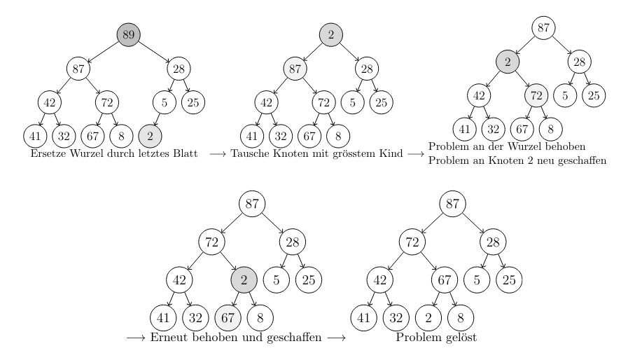
Current
Note has been deleted
Field-by-field Comparison
| Field | Before | After |
|---|---|---|
| Front | ||
| Back |
Note 173: ETH::1. Semester::A&D
Deck: ETH::1. Semester::A&D
Note Type: Horvath Cloze
GUID:
deleted
Note Type: Horvath Cloze
GUID:
fT7%2bq&hL
Deleted Note
Front
In BFS enter/leave ordering for all \(v\), enter[v] < leave[v].
Back
In BFS enter/leave ordering for all \(v\), enter[v] < leave[v].
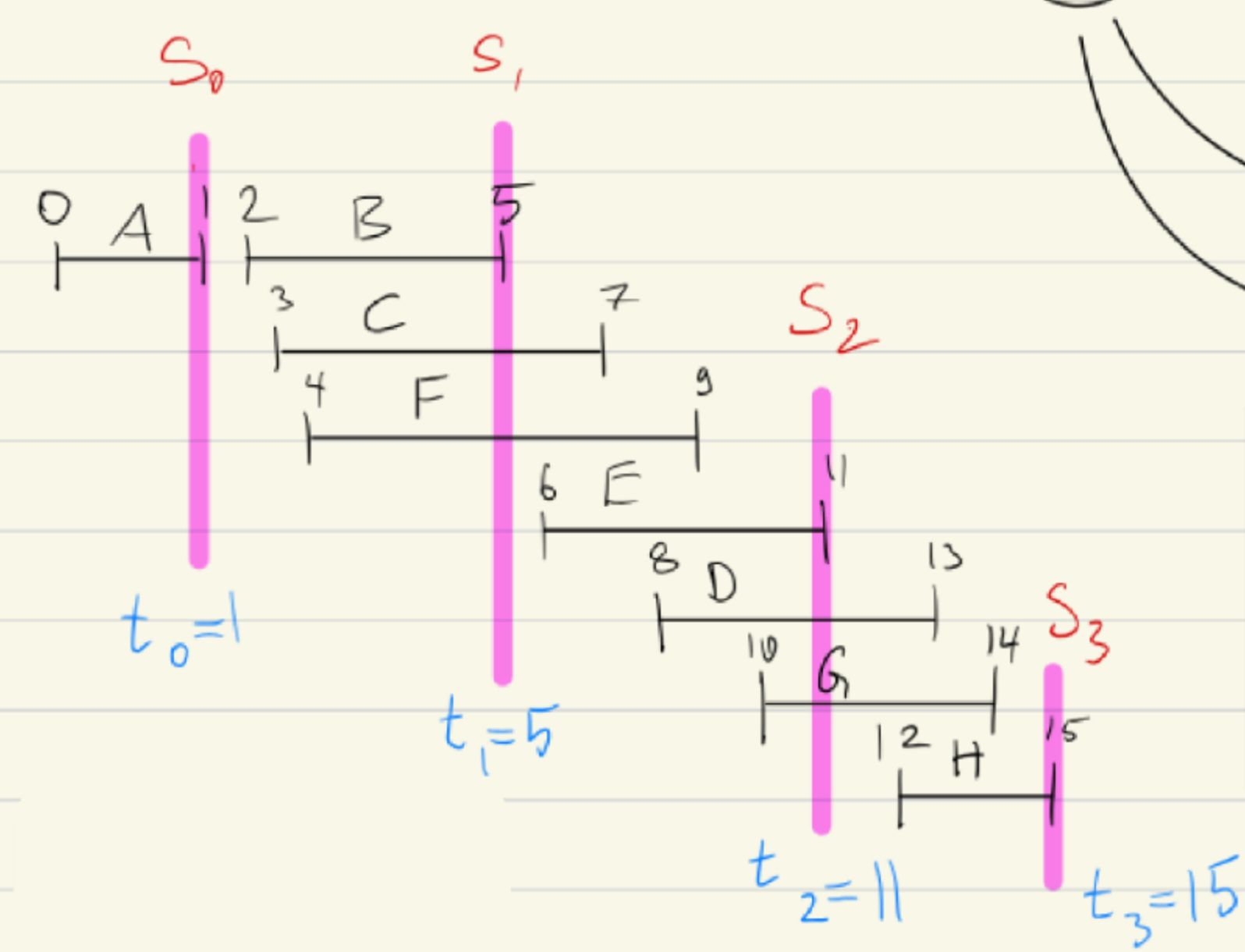
Current
Note has been deleted
Field-by-field Comparison
| Field | Before | After |
|---|---|---|
| Text | ||
| Extra |
Note 174: ETH::1. Semester::A&D
Deck: ETH::1. Semester::A&D
Note Type: Horvath Classic
GUID:
deleted
Note Type: Horvath Classic
GUID:
fa/9a*g+D.
Deleted Note
Front
How can one get a lower bound for the function \(n!\) ?
Back
How can one get a lower bound for the function \(n!\) ?
One could simply take only the largest 90% of elements: \(n! \geq 1 \cdot 2 \cdot ... \cdot n \geq n/10 \cdot ... \cdot n\)
\(\geq (n/10)^{0.9n}\)
Current
Note has been deleted
Field-by-field Comparison
| Field | Before | After |
|---|---|---|
| Front | ||
| Back |
Note 175: ETH::1. Semester::A&D
Deck: ETH::1. Semester::A&D
Note Type: Horvath Classic
GUID:
deleted
Note Type: Horvath Classic
GUID:
g$?N5#OWTc
Deleted Note
Front
How do we know if a walk \(W=(v_0, ..., v_n)\) is closed using the degree of \(v_n\) in \(W\)?
Back
How do we know if a walk \(W=(v_0, ..., v_n)\) is closed using the degree of \(v_n\) in \(W\)?
it is closed if and only if \(\text{deg}_W(v_n)\) is even
every occurrence of \(v_n\) within the walk increases its degree by 2, so it does not affect parity so if the degree is even then \(v_n\) is both the first and the last node
every occurrence of \(v_n\) within the walk increases its degree by 2, so it does not affect parity so if the degree is even then \(v_n\) is both the first and the last node
Current
Note has been deleted
Field-by-field Comparison
| Field | Before | After |
|---|---|---|
| Front | ||
| Back |
Note 176: ETH::1. Semester::A&D
Deck: ETH::1. Semester::A&D
Note Type: Horvath Classic
GUID:
deleted
Note Type: Horvath Classic
GUID:
gCxT2!W2sa
Deleted Note
Front
Runtime of DFS with matrix vs list:
Back
Runtime of DFS with matrix vs list:
\(n\) calls to visit. Each takes:
- Matrix: \(O(n)\) as we loop edges gives \(n \cdot O(n) = O(n^2)\)
- List: \(O(1 + \deg_{out}(u))\) gives \(n \cdot O(1 + \deg_{out}(v) = |V| + |E|\)
Current
Note has been deleted
Field-by-field Comparison
| Field | Before | After |
|---|---|---|
| Front | ||
| Back |
Note 177: ETH::1. Semester::A&D
Deck: ETH::1. Semester::A&D
Note Type: Algorithms
GUID:
deleted
Note Type: Algorithms
GUID:
gE_4/z}oud
Deleted Note
Front
Runtime of Edit Distance?
Back
Runtime of Edit Distance?
\(\Theta(n \cdot m)\)
Current
Note has been deleted
Field-by-field Comparison
| Field | Before | After |
|---|---|---|
| Name | ||
| Runtime | ||
| Approach | ||
| Pseudocode |
Note 178: ETH::1. Semester::A&D
Deck: ETH::1. Semester::A&D
Note Type: Horvath Cloze
GUID:
deleted
Note Type: Horvath Cloze
GUID:
gW55x`wH1(
Deleted Note
Front
A vertex with {{c1::\(\deg_{\text{in} }(v) = 0\)}} is called a source (Quelle).
Back
A vertex with {{c1::\(\deg_{\text{in} }(v) = 0\)}} is called a source (Quelle).
Current
Note has been deleted
Field-by-field Comparison
| Field | Before | After |
|---|---|---|
| Text |
Note 179: ETH::1. Semester::A&D
Deck: ETH::1. Semester::A&D
Note Type: Horvath Cloze
GUID:
deleted
Note Type: Horvath Cloze
GUID:
ge[wn7-Qb.
Deleted Note
Front
Kadane's algorithm solves the Maximum Subarray Sum (MSS) problem in {{c2::linear (\(\mathcal{O}(n)\))}} time.
Back
Kadane's algorithm solves the Maximum Subarray Sum (MSS) problem in {{c2::linear (\(\mathcal{O}(n)\))}} time.
This is the optimal solution for MSS.
Current
Note has been deleted
Field-by-field Comparison
| Field | Before | After |
|---|---|---|
| Text | ||
| Extra |
Note 180: ETH::1. Semester::A&D
Deck: ETH::1. Semester::A&D
Note Type: Horvath Classic
GUID:
deleted
Note Type: Horvath Classic
GUID:
gm7WcQEU/C
Deleted Note
Front
When do we want Dijkstra's with an array?
Back
When do we want Dijkstra's with an array?
In very dense graphs\(|E| > \frac{|V|^2}{\log |V|}\), Dijkstra's is faster on an array than in a minHeap.
Extract_min takes \(O(|V|)\) with an array (\(O(\log |V|)\) in a MinHeap) -> array implementation runtime: \(O(|V|^2 + |E|) = O(|V|^2)\) for \(|E| = \Theta(|V|^2)\) (there are at most \(|V|^2\) edges in a graph).
If we plug in |E| > ... into the log runtime we see it's faster.
Current
Note has been deleted
Field-by-field Comparison
| Field | Before | After |
|---|---|---|
| Front | ||
| Back |
Note 181: ETH::1. Semester::A&D
Deck: ETH::1. Semester::A&D
Note Type: Horvath Classic
GUID:
deleted
Note Type: Horvath Classic
GUID:
g}Fn_v+#@3
Deleted Note
Front
What is the Cut-Property (Schnittprinzip)?
Back
What is the Cut-Property (Schnittprinzip)?
To join a set of disjoint connected components, we need to use an edge to join two of their vertices. The idea is that the cheapest such edge is always a safe edge.
This is true only for distinct edge weights!
Current
Note has been deleted
Field-by-field Comparison
| Field | Before | After |
|---|---|---|
| Front | ||
| Back |
Note 182: ETH::1. Semester::A&D
Deck: ETH::1. Semester::A&D
Note Type: Algorithms
GUID:
deleted
Note Type: Algorithms
GUID:
hL7UB-)y6N
Deleted Note
Front
Runtime of Floyd-Warshall?
Back
Runtime of Floyd-Warshall?
\(O(|V|^3)\)
Current
Note has been deleted
Field-by-field Comparison
| Field | Before | After |
|---|---|---|
| Name | ||
| Runtime | ||
| Requirements | ||
| Approach | ||
| Pseudocode | ||
| Use Case |
Note 183: ETH::1. Semester::A&D
Deck: ETH::1. Semester::A&D
Note Type: Horvath Cloze
GUID:
deleted
Note Type: Horvath Cloze
GUID:
hsaD+h{~n8
Deleted Note
Front
Reweighting in Johnson's algorithm:
- We add a vertex \(s\) and add a 0 cost edge from it to all vertices.
- We then run Bellman-Ford which determines the height of each vertex by the d[v] from start vertex \(s\)
Back
Reweighting in Johnson's algorithm:
- We add a vertex \(s\) and add a 0 cost edge from it to all vertices.
- We then run Bellman-Ford which determines the height of each vertex by the d[v] from start vertex \(s\)
Current
Note has been deleted
Field-by-field Comparison
| Field | Before | After |
|---|---|---|
| Text |
Note 184: ETH::1. Semester::A&D
Deck: ETH::1. Semester::A&D
Note Type: Horvath Cloze
GUID:
deleted
Note Type: Horvath Cloze
GUID:
hv)-{h!@?x
Deleted Note
Front
The amortised runtime of union in the Union-Find datastructure is \(O(|V| \log |V|)\).
Back
The amortised runtime of union in the Union-Find datastructure is \(O(|V| \log |V|)\).
Union takes \(\Theta(\min \{ |ZHK(u)| , |ZHK(v)| \}\). In the worst case, the minimum is \(|V| / 2\) as both have the same size.
Therefore over all loops, this would take \(O(|V| \log |V|)\) time, as on average we only take \(O(\log |V|)\) time.
The graph stays worst case, this is the average of the calls in the worst case.
Therefore over all loops, this would take \(O(|V| \log |V|)\) time, as on average we only take \(O(\log |V|)\) time.
The graph stays worst case, this is the average of the calls in the worst case.
Current
Note has been deleted
Field-by-field Comparison
| Field | Before | After |
|---|---|---|
| Text | ||
| Extra |
Note 185: ETH::1. Semester::A&D
Deck: ETH::1. Semester::A&D
Note Type: Horvath Cloze
GUID:
deleted
Note Type: Horvath Cloze
GUID:
i3K1KB$5&t
Deleted Note
Front
{{c1::\(\sum_{i = 1}^{n} \sum_{i = 1}^{n} 1\)::Sum}} \(=\) \(n^2\)
Back
{{c1::\(\sum_{i = 1}^{n} \sum_{i = 1}^{n} 1\)::Sum}} \(=\) \(n^2\)
Current
Note has been deleted
Field-by-field Comparison
| Field | Before | After |
|---|---|---|
| Text |
Note 186: ETH::1. Semester::A&D
Deck: ETH::1. Semester::A&D
Note Type: Horvath Cloze
GUID:
deleted
Note Type: Horvath Cloze
GUID:
i6hHee%a$O
Deleted Note
Front
Choose a tight bound!
\(O(n!) \leq O(n^n)\)
\(O(n!) \leq O(n^n)\)
Back
Choose a tight bound!
\(O(n!) \leq O(n^n)\)
\(O(n!) \leq O(n^n)\)
Current
Note has been deleted
Field-by-field Comparison
| Field | Before | After |
|---|---|---|
| Text |
Note 187: ETH::1. Semester::A&D
Deck: ETH::1. Semester::A&D
Note Type: Horvath Cloze
GUID:
deleted
Note Type: Horvath Cloze
GUID:
iFt.dzS26%
Deleted Note
Front
A graph \(G\) is transitive when for {{c2::any two edges \(\{u, v\} \text{ and } \{v, w\}\) in \(E\), the edge \(\{u, w\}\) is also in \(E\)}}.
Back
A graph \(G\) is transitive when for {{c2::any two edges \(\{u, v\} \text{ and } \{v, w\}\) in \(E\), the edge \(\{u, w\}\) is also in \(E\)}}.
Current
Note has been deleted
Field-by-field Comparison
| Field | Before | After |
|---|---|---|
| Text |
Note 188: ETH::1. Semester::A&D
Deck: ETH::1. Semester::A&D
Note Type: Horvath Cloze
GUID:
deleted
Note Type: Horvath Cloze
GUID:
iHlSvEEQPk
Deleted Note
Front
A graph \(G\) is complete when it's set of edges is {{c2::\(\{\{u, v\} \ | \ u, v \in V, u \neq v\}\) }}.
Back
A graph \(G\) is complete when it's set of edges is {{c2::\(\{\{u, v\} \ | \ u, v \in V, u \neq v\}\) }}.
Current
Note has been deleted
Field-by-field Comparison
| Field | Before | After |
|---|---|---|
| Text |
Note 189: ETH::1. Semester::A&D
Deck: ETH::1. Semester::A&D
Note Type: Horvath Cloze
GUID:
deleted
Note Type: Horvath Cloze
GUID:
i`Yd8WTI?B
Deleted Note
Front
There's no MST if the graph is disconnected.
Back
There's no MST if the graph is disconnected.
Current
Note has been deleted
Field-by-field Comparison
| Field | Before | After |
|---|---|---|
| Text |
Note 190: ETH::1. Semester::A&D
Deck: ETH::1. Semester::A&D
Note Type: Horvath Classic
GUID:
deleted
Note Type: Horvath Classic
GUID:
ij#NQ.@u}5
Deleted Note
Front
Is it possible to use the master theorem to get \(\Theta(f)\)? How?
Back
Is it possible to use the master theorem to get \(\Theta(f)\)? How?
for a recursive function if both the Master theorem for the upper bound on the runtime and the lower bound on the runtime hold, then \(T(n) = \Theta(n^b), \Theta(n^{\log_2 a}\log n), \Theta(n^{\log_2 a})\) respectively for the three cases
Current
Note has been deleted
Field-by-field Comparison
| Field | Before | After |
|---|---|---|
| Front | ||
| Back |
Note 191: ETH::1. Semester::A&D
Deck: ETH::1. Semester::A&D
Note Type: Horvath Cloze
GUID:
deleted
Note Type: Horvath Cloze
GUID:
i|cJp0X3s*
Deleted Note
Front
A graph \(G\) is connected (Zusammenhängend) if for every two vertices \(u, v \in V\) \(u\) reaches \(v\).
Back
A graph \(G\) is connected (Zusammenhängend) if for every two vertices \(u, v \in V\) \(u\) reaches \(v\).
Current
Note has been deleted
Field-by-field Comparison
| Field | Before | After |
|---|---|---|
| Text |
Note 192: ETH::1. Semester::A&D
Deck: ETH::1. Semester::A&D
Note Type: Horvath Classic
GUID:
deleted
Note Type: Horvath Classic
GUID:
i~[|jYI|rt
Deleted Note
Front
What is "backtracking" in DP problems?
Back
What is "backtracking" in DP problems?
Once the DP table is filled, backtracking reconstructs the actual solution (not just the optimal value) by tracing which choices led to each cell.
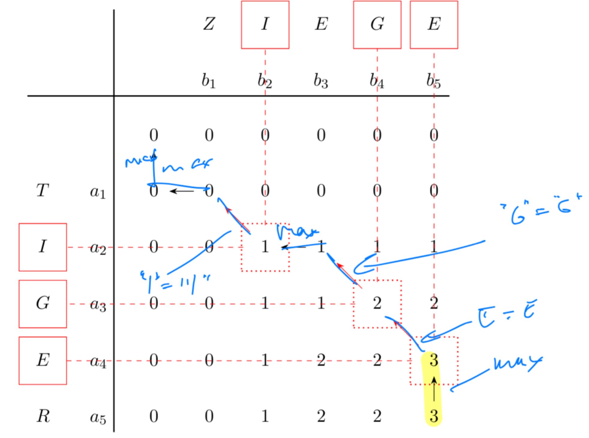
Current
Note has been deleted
Field-by-field Comparison
| Field | Before | After |
|---|---|---|
| Front | ||
| Back |
Note 193: ETH::1. Semester::A&D
Deck: ETH::1. Semester::A&D
Note Type: Algorithms
GUID:
deleted
Note Type: Algorithms
GUID:
j#w5w>dS6
Deleted Note
Front
Back
Runtime of
Bellman-Ford
Runtime: :\( \mathcal{O}(|E| \cdot |V|)\)}}
Approach: Initiate all distances with \(\infty\) . Then go \(|V| - 1\) times through every edge, and test for all (u,v) in E if \(\text{dist}[v] > \text{dist}[u] + w(u,v)\). If yes, update the distance. If after \(|V| - 1\) iterations an edge can still be relaxed (in a last iteration), then there exists a negative cycle
Uses: Detect negative cycles, find minimal-cost paths in weighted graphs with negative weights}}
?Current
Note has been deleted
Field-by-field Comparison
| Field | Before | After |
|---|---|---|
| Name |
Note 194: ETH::1. Semester::A&D
Deck: ETH::1. Semester::A&D
Note Type: Horvath Classic
GUID:
deleted
Note Type: Horvath Classic
GUID:
j+9WeY4$!x
Deleted Note
Front
Explain why reweighting in Johnson's algorithm works:
Back
Explain why reweighting in Johnson's algorithm works:
Assigns a height \(h(v)\) to each vertex. The new cost is then \(\hat{c}(u, v) = c(u, v) + h(u) - h(v)\).
For a path \(P = (s, v_1, v_2, \dots, v_n, t)\) the cost \(\hat{c}(P) = \hat{c}(s, v_1) + \hat{c}(v_1, v_2) + \dots + \hat{c}(v_n, t)\) the costs cancel out in pairs: \(c(s, v_1) + h(s) - h(v_1) + c(v_1, v_2) + h(v_1) - h(v_2) + \dots + c(v_n, t) + h(v_n) - h(t)\) gives \(= c(P) + h(s) - h(t)\), which satisfies our requirements that the ordering stay the same.
For a path \(P = (s, v_1, v_2, \dots, v_n, t)\) the cost \(\hat{c}(P) = \hat{c}(s, v_1) + \hat{c}(v_1, v_2) + \dots + \hat{c}(v_n, t)\) the costs cancel out in pairs: \(c(s, v_1) + h(s) - h(v_1) + c(v_1, v_2) + h(v_1) - h(v_2) + \dots + c(v_n, t) + h(v_n) - h(t)\) gives \(= c(P) + h(s) - h(t)\), which satisfies our requirements that the ordering stay the same.
Current
Note has been deleted
Field-by-field Comparison
| Field | Before | After |
|---|---|---|
| Front | ||
| Back |
Note 195: ETH::1. Semester::A&D
Deck: ETH::1. Semester::A&D
Note Type: Horvath Cloze
GUID:
deleted
Note Type: Horvath Cloze
GUID:
jBru?ce!L0
Deleted Note
Front
We use Floyd-Warshall over Johnsons, when the graph is very dense \(|E| = \Theta(|V|^2)\).
Back
We use Floyd-Warshall over Johnsons, when the graph is very dense \(|E| = \Theta(|V|^2)\).
Then the \(n \cdot (n + m) \) becomes \(n \cdot (n + n^2)\) which is \(O(n^3)\).
Current
Note has been deleted
Field-by-field Comparison
| Field | Before | After |
|---|---|---|
| Text | ||
| Extra |
Note 196: ETH::1. Semester::A&D
Deck: ETH::1. Semester::A&D
Note Type: Algorithms
GUID:
deleted
Note Type: Algorithms
GUID:
jcougdQ#0G
Deleted Note
Front
Back
Runtime of
Kruskal
Runtime: {{c1::\( \mathcal{O}(|E| \log |E| + |E| \log|V|)\)}}
Approach:
Uses:
?Current
Note has been deleted
Field-by-field Comparison
| Field | Before | After |
|---|---|---|
| Name |
Note 197: ETH::1. Semester::A&D
Deck: ETH::1. Semester::A&D
Note Type: Horvath Classic
GUID:
deleted
Note Type: Horvath Classic
GUID:
jj%LAs_%qo
Deleted Note
Front
Pre- and Postordering in BFS:
Back
Pre- and Postordering in BFS:
Same as with pre-/postordering, we can use enter-/leave-ordering here:
enterstep at which vertex \(v\) is first encountered.leavestep at which vertex \(v\) is dequeued
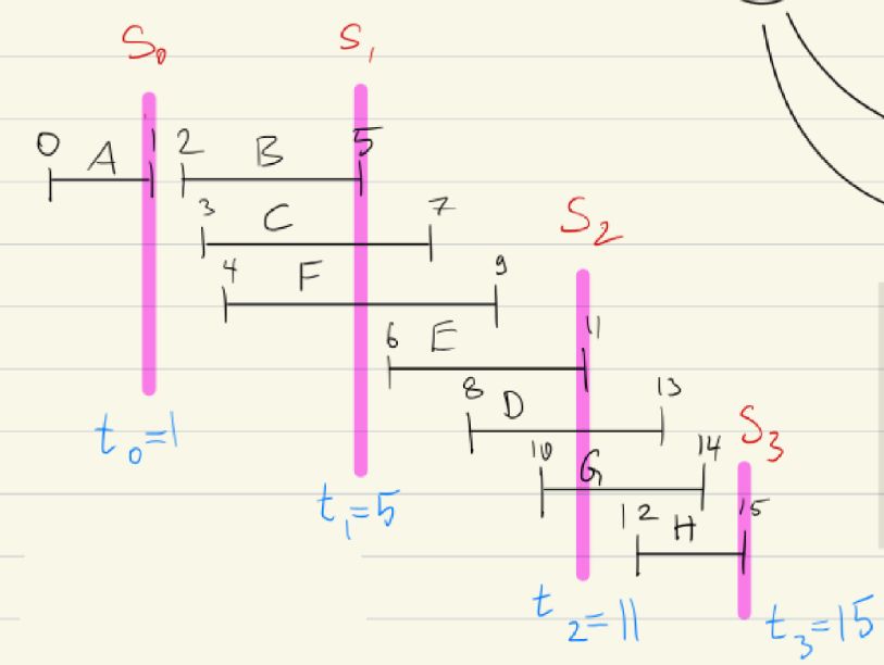
Current
Note has been deleted
Field-by-field Comparison
| Field | Before | After |
|---|---|---|
| Front | ||
| Back |
Note 198: ETH::1. Semester::A&D
Deck: ETH::1. Semester::A&D
Note Type: Horvath Classic
GUID:
deleted
Note Type: Horvath Classic
GUID:
jp(fyg:?5N
Deleted Note
Front
What is the mathematical definition of a graph?
Back
What is the mathematical definition of a graph?
\(G = (V, E)\) with \(V\) the set of all vertices (Knotenmenge) and \(E\) the set of all edges (Kantenmenge).
Current
Note has been deleted
Field-by-field Comparison
| Field | Before | After |
|---|---|---|
| Front | ||
| Back |
Note 199: ETH::1. Semester::A&D
Deck: ETH::1. Semester::A&D
Note Type: Horvath Cloze
GUID:
deleted
Note Type: Horvath Cloze
GUID:
k#~pL>w{_$
Deleted Note
Front
What are the prerequisites for \(f\) and \(g\) to apply l'Hôpital's?
- \(f, g\) are differentiable (for sufficiently large \(x\))
- {{c2::\(\lim_{x \to \infty} f(x) = \lim_{x \to \infty} g(x) = \infty\) (or both \(= 0\))}}
- \(g'(x) \neq 0\) for sufficiently large \(x\)
- {{c4::\(\lim_{x \to \infty} \frac{f'(x)}{g'(x)}\) exists (or is \(\pm \infty\))}}
Back
What are the prerequisites for \(f\) and \(g\) to apply l'Hôpital's?
- \(f, g\) are differentiable (for sufficiently large \(x\))
- {{c2::\(\lim_{x \to \infty} f(x) = \lim_{x \to \infty} g(x) = \infty\) (or both \(= 0\))}}
- \(g'(x) \neq 0\) for sufficiently large \(x\)
- {{c4::\(\lim_{x \to \infty} \frac{f'(x)}{g'(x)}\) exists (or is \(\pm \infty\))}}
Then: \(\lim_{x \to \infty} \frac{f(x)}{g(x)} = \lim_{x \to \infty} \frac{f'(x)}{g'(x)}\)
Current
Note has been deleted
Field-by-field Comparison
| Field | Before | After |
|---|---|---|
| Text | ||
| Extra |
Note 200: ETH::1. Semester::A&D
Deck: ETH::1. Semester::A&D
Note Type: Horvath Classic
GUID:
deleted
Note Type: Horvath Classic
GUID:
k%duL(GzS|
Deleted Note
Front
In every connected graph \(G\), when executing Kruskal using Union-Find, the representative repr[u] changes \(O(\dots)\) times:
Back
In every connected graph \(G\), when executing Kruskal using Union-Find, the representative repr[u] changes \(O(\dots)\) times:
\(O(\log_2 |V|)\), as we always at least double the size of the representative (we merge smaller into bigger, and repr[u] changes if it's the smaller one).
Current
Note has been deleted
Field-by-field Comparison
| Field | Before | After |
|---|---|---|
| Front | ||
| Back |
Note 201: ETH::1. Semester::A&D
Deck: ETH::1. Semester::A&D
Note Type: Horvath Cloze
GUID:
deleted
Note Type: Horvath Cloze
GUID:
kCvO2]PU.a
Deleted Note
Front
\(\ln(1)= {{c1:: 0::\text{Number} }}\)
Back
\(\ln(1)= {{c1:: 0::\text{Number} }}\)
Current
Note has been deleted
Field-by-field Comparison
| Field | Before | After |
|---|---|---|
| Text |
Note 202: ETH::1. Semester::A&D
Deck: ETH::1. Semester::A&D
Note Type: Horvath Cloze
GUID:
deleted
Note Type: Horvath Cloze
GUID:
kR-q@1!eo3
Deleted Note
Front
The runtime of search in a binary tree is \(O(h)\), where \(h\) is the height.
Back
The runtime of search in a binary tree is \(O(h)\), where \(h\) is the height.
Current
Note has been deleted
Field-by-field Comparison
| Field | Before | After |
|---|---|---|
| Text |
Note 203: ETH::1. Semester::A&D
Deck: ETH::1. Semester::A&D
Note Type: Horvath Classic
GUID:
deleted
Note Type: Horvath Classic
GUID:
kXVME,u35.
Deleted Note
Front
What's the space complexity of merge sort?
Back
What's the space complexity of merge sort?
\(O(n)\)
Current
Note has been deleted
Field-by-field Comparison
| Field | Before | After |
|---|---|---|
| Front | ||
| Back |
Note 204: ETH::1. Semester::A&D
Deck: ETH::1. Semester::A&D
Note Type: Algorithms
GUID:
deleted
Note Type: Algorithms
GUID:
kn@H8`z>0t
Deleted Note
Front
Runtime of DFS (Depth First Search)?
Back
Runtime of DFS (Depth First Search)?
\( \mathcal{O}(|E| + |V|) \) (using Adjacency List)
Can be efficiently implemented using a stack.
Can be efficiently implemented using a stack.
Current
Note has been deleted
Field-by-field Comparison
| Field | Before | After |
|---|---|---|
| Name | ||
| Runtime | ||
| Approach | ||
| Pseudocode | ||
| Use Case | ||
| Extra Info |
Note 205: ETH::1. Semester::A&D
Deck: ETH::1. Semester::A&D
Note Type: Horvath Reverso
GUID:
deleted
Note Type: Horvath Reverso
GUID:
l2vPmFwTj!
Deleted Note
Front
Subsequence
Back
Subsequence
Teilfolge
Current
Note has been deleted
Field-by-field Comparison
| Field | Before | After |
|---|---|---|
| Front | ||
| Back |
Note 206: ETH::1. Semester::A&D
Deck: ETH::1. Semester::A&D
Note Type: Horvath Cloze
GUID:
deleted
Note Type: Horvath Cloze
GUID:
l`x
Deleted Note
Front
\(\ln(2) - 1 < 0\)
Back
\(\ln(2) - 1 < 0\)
We have \(\ln(2) \sim 0.67\) thus it's negative.
Current
Note has been deleted
Field-by-field Comparison
| Field | Before | After |
|---|---|---|
| Text | ||
| Extra |
Note 207: ETH::1. Semester::A&D
Deck: ETH::1. Semester::A&D
Note Type: Horvath Classic
GUID:
deleted
Note Type: Horvath Classic
GUID:
lg2TVeS_j]
Deleted Note
Front
How can I find the asymptotic behavior of a sum like \(\sum_{i = 1}^{^{\lceil \sqrt{n} \rceil}} \sqrt{i}\)?
Back
How can I find the asymptotic behavior of a sum like \(\sum_{i = 1}^{^{\lceil \sqrt{n} \rceil}} \sqrt{i}\)?
Sum and integral have the same asymptotic behavior (not covered in lecture)!
\[\begin{align} \sum_{i=1}^{\lceil \sqrt{n} \rceil} \sqrt{i} &\sim \int_1^{\lceil \sqrt{n} \rceil} \sqrt{x}\,dx \\ &= \left[\frac{2}{3}x^{3/2}\right]_1^{\lceil \sqrt{n} \rceil} \\ &= \frac{2}{3}\bigl(\lceil \sqrt{n} \rceil^{3/2} - 1\bigr) \\ &\sim \frac{2}{3}\bigl(n^{1/2}\bigr)^{3/2} \\ &= \Theta(n^{3/4}). \end{align}\]
(We use \(\sim\) to denote asympotic equivalence. Correct but verbose would be to wrap everything in \(\Theta\))
Current
Note has been deleted
Field-by-field Comparison
| Field | Before | After |
|---|---|---|
| Front | ||
| Back |
Note 208: ETH::1. Semester::A&D
Deck: ETH::1. Semester::A&D
Note Type: Horvath Classic
GUID:
deleted
Note Type: Horvath Classic
GUID:
ll$H=f;!5
Deleted Note
Front
Which functions \(f(n)\) have \(\lim_{n\rightarrow \infty} f(n)\) undefined?
Back
Which functions \(f(n)\) have \(\lim_{n\rightarrow \infty} f(n)\) undefined?
Typically functions that oscilate as they approach infinity such as \(f(n) = \sin n\) or \(f(n) = (-1)^n\)
Current
Note has been deleted
Field-by-field Comparison
| Field | Before | After |
|---|---|---|
| Front | ||
| Back |
Note 209: ETH::1. Semester::A&D
Deck: ETH::1. Semester::A&D
Note Type: Horvath Classic
GUID:
deleted
Note Type: Horvath Classic
GUID:
m3`Qbb~x?c
Deleted Note
Front
2-3 Tree: We deleted a node and now it's sibling is an only child. What happens if it's neighbor has 3 keys?
Back
2-3 Tree: We deleted a node and now it's sibling is an only child. What happens if it's neighbor has 3 keys?
Our current node adopts one of the children. The separators have to be updated by “rotating them”. The parent sep moves with the adopted and the left sep becomes the new parent).
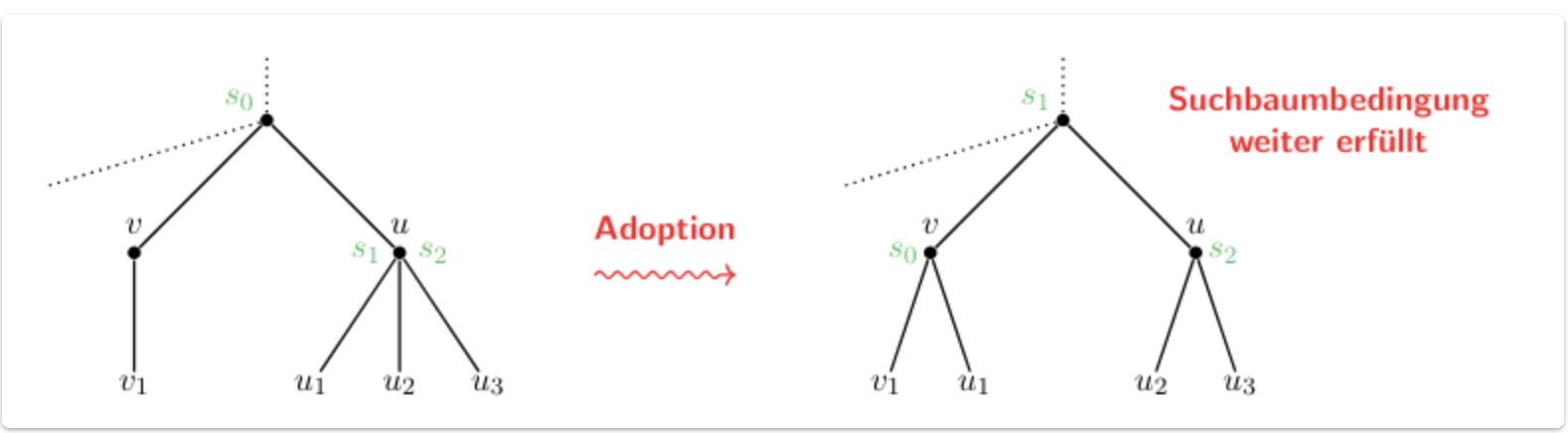
Current
Note has been deleted
Field-by-field Comparison
| Field | Before | After |
|---|---|---|
| Front | ||
| Back |
Note 210: ETH::1. Semester::A&D
Deck: ETH::1. Semester::A&D
Note Type: Horvath Classic
GUID:
deleted
Note Type: Horvath Classic
GUID:
m5TC:^C`Y9
Deleted Note
Front
How to speed up array access for a DP-array
Back
How to speed up array access for a DP-array
Row-Major vs. Column Major Access:
Set the inner loop variable to be the array's inner variable:
for j in ...:
for i in ...:
DP[j][i]
Otherwise we have to jump DP[i].length elements each time we want to access the next element.
Set the inner loop variable to be the array's inner variable:
for j in ...:
for i in ...:
DP[j][i]
Otherwise we have to jump DP[i].length elements each time we want to access the next element.
Current
Note has been deleted
Field-by-field Comparison
| Field | Before | After |
|---|---|---|
| Front | ||
| Back |
Note 211: ETH::1. Semester::A&D
Deck: ETH::1. Semester::A&D
Note Type: Horvath Cloze
GUID:
deleted
Note Type: Horvath Cloze
GUID:
m@n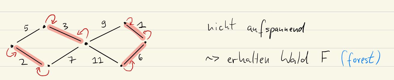
- Now, repeat by finding the cheapest outgoing edge for each component. Do this until all are connected.
- \(F\) constitutes the edges of the MST.
Current
Note has been deleted
Field-by-field Comparison
| Field | Before | After |
|---|---|---|
| Front | ||
| Back |
Note 216: ETH::1. Semester::A&D
Deck: ETH::1. Semester::A&D
Note Type: Algorithms
GUID:
deleted
Note Type: Algorithms
GUID:
m`oj
Deleted Note
Front
Runtime of Prim's Algorithm?
Back
Runtime of Prim's Algorithm?
\(O((|V| + |E|) \log |V|)\) (Adjacency List, otherwise \(\Theta(|V|^2)\) like Dijkstra's)
Current
Note has been deleted
Field-by-field Comparison
| Field | Before | After |
|---|---|---|
| Name | ||
| Runtime | ||
| Requirements | ||
| Approach | ||
| Pseudocode | ||
| Use Case |
Note 217: ETH::1. Semester::A&D
Deck: ETH::1. Semester::A&D
Note Type: Horvath Classic
GUID:
deleted
Note Type: Horvath Classic
GUID:
mabS@W|F#G
Deleted Note
Front
Explain how to find a topological order (high-level):
Back
Explain how to find a topological order (high-level):
We can build one backwards, by always finding a vertex which has no succeeding vertices, removing it from the graph and adding it to the front of our topologically sorted list.
This is not possible if there is a directed cycle in the graph.
This is not possible if there is a directed cycle in the graph.
Current
Note has been deleted
Field-by-field Comparison
| Field | Before | After |
|---|---|---|
| Front | ||
| Back |
Note 218: ETH::1. Semester::A&D
Deck: ETH::1. Semester::A&D
Note Type: Horvath Cloze
GUID:
deleted
Note Type: Horvath Cloze
GUID:
mhrX@w|*.`
Deleted Note
Front
In graph theory, an Eulerian walk (Eulerweg) is a walk that contains every edge of the graph exactly once.
Back
In graph theory, an Eulerian walk (Eulerweg) is a walk that contains every edge of the graph exactly once.
Current
Note has been deleted
Field-by-field Comparison
| Field | Before | After |
|---|---|---|
| Text |
Note 219: ETH::1. Semester::A&D
Deck: ETH::1. Semester::A&D
Note Type: Horvath Classic
GUID:
deleted
Note Type: Horvath Classic
GUID:
ms|2]oAD;M
Deleted Note
Front
If \(T(n) = aT(n/ 2) + Cn^b\), then we get which type of O-Notation?
Back
If \(T(n) = aT(n/ 2) + Cn^b\), then we get which type of O-Notation?
\(T(n) = \Theta(...)\)
Current
Note has been deleted
Field-by-field Comparison
| Field | Before | After |
|---|---|---|
| Front | ||
| Back |
Note 220: ETH::1. Semester::A&D
Deck: ETH::1. Semester::A&D
Note Type: Horvath Classic
GUID:
deleted
Note Type: Horvath Classic
GUID:
m{e.+pS,Zn
Deleted Note
Front
How can you find the upper bound of a geometric series like \(T = 7^1, 7^2, \ldots, 7^n\)?
Back
How can you find the upper bound of a geometric series like \(T = 7^1, 7^2, \ldots, 7^n\)?
Use the multiply-subract trick.
- Mutliply the series by its base: \(7T\)
- Subtract: \(7T - T = 7^{n+1} - 7^1\) (middle terms cancel)
- Factor: \(T(7-1) = 7^{n+1} - 7^1\)
- Divide: \(T = \frac{7^{n+1} - 7^1}{6}\)
This trick works even if every term has a constant coefficient.
Current
Note has been deleted
Field-by-field Comparison
| Field | Before | After |
|---|---|---|
| Front | ||
| Back |
Note 221: ETH::1. Semester::A&D
Deck: ETH::1. Semester::A&D
Note Type: Horvath Cloze
GUID:
deleted
Note Type: Horvath Cloze
GUID:
n!`Y!GEmVs
Deleted Note
Front
{{c1:: \(\sum_{i = 1}^{n} i\)::Sum}} \(=\) {{c2::\(\frac{n(n + 1)}{2}\)}}
Back
{{c1:: \(\sum_{i = 1}^{n} i\)::Sum}} \(=\) {{c2::\(\frac{n(n + 1)}{2}\)}}
Current
Note has been deleted
Field-by-field Comparison
| Field | Before | After |
|---|---|---|
| Text |
Note 222: ETH::1. Semester::A&D
Deck: ETH::1. Semester::A&D
Note Type: Horvath Cloze
GUID:
deleted
Note Type: Horvath Cloze
GUID:
n/PBpw~:i9
Deleted Note
Front
We can use a binary search tree to implement the dictionary.
The tree-condition is for every node, all keys in the left child are smaller than those in the right child.
The tree-condition is for every node, all keys in the left child are smaller than those in the right child.
Back
We can use a binary search tree to implement the dictionary.
The tree-condition is for every node, all keys in the left child are smaller than those in the right child.
The tree-condition is for every node, all keys in the left child are smaller than those in the right child.
Current
Note has been deleted
Field-by-field Comparison
| Field | Before | After |
|---|---|---|
| Text |
Note 223: ETH::1. Semester::A&D
Deck: ETH::1. Semester::A&D
Note Type: Horvath Cloze
GUID:
deleted
Note Type: Horvath Cloze
GUID:
n=wUJ;@Xl(
Deleted Note
Front
In BFS enter/leave ordering, the FIFO queue guarantees that the enter order equals the leave order within a given level.
Back
In BFS enter/leave ordering, the FIFO queue guarantees that the enter order equals the leave order within a given level.
Current
Note has been deleted
Field-by-field Comparison
| Field | Before | After |
|---|---|---|
| Text | ||
| Extra |
Note 224: ETH::1. Semester::A&D
Deck: ETH::1. Semester::A&D
Note Type: Horvath Cloze
GUID:
deleted
Note Type: Horvath Cloze
GUID:
nK{)v6I%zc
Deleted Note
Front
The ADT stack can be efficiently implemented using a singly linked list:
- push: \(\Theta(1)\)
- pop: \(\Theta(1)\) as this removes the first element. This means we just copy the pointer next from the first element to be the first pointer of the list.
Back
The ADT stack can be efficiently implemented using a singly linked list:
- push: \(\Theta(1)\)
- pop: \(\Theta(1)\) as this removes the first element. This means we just copy the pointer next from the first element to be the first pointer of the list.
Current
Note has been deleted
Field-by-field Comparison
| Field | Before | After |
|---|---|---|
| Text |
Note 225: ETH::1. Semester::A&D
Deck: ETH::1. Semester::A&D
Note Type: Algorithms
GUID:
deleted
Note Type: Algorithms
GUID:
nb9;e*.#MD
Deleted Note
Front
Back
Runtime of Heapsort?
Current
Note has been deleted
Field-by-field Comparison
| Field | Before | After |
|---|---|---|
| Name | ||
| Approach | ||
| Pseudocode | ||
| Invariant | ||
| Attributes |
Note 226: ETH::1. Semester::A&D
Deck: ETH::1. Semester::A&D
Note Type: Algorithms
GUID:
deleted
Note Type: Algorithms
GUID:
nfdJ7OmBdJ
Deleted Note
Front
Back
Runtime of
Floyd-Warshall
Runtime: {{c1::\( \mathcal{O}(|V|^3)\)}}
Approach:
Uses:
?Current
Note has been deleted
Field-by-field Comparison
| Field | Before | After |
|---|---|---|
| Name |
Note 227: ETH::1. Semester::A&D
Deck: ETH::1. Semester::A&D
Note Type: Horvath Cloze
GUID:
deleted
Note Type: Horvath Cloze
GUID:
nmO79UYMKA
Deleted Note
Front
DFS Pseudocode needs to include a for loop over all unmarked nodes, when we're not sure whether the graph is connected.
Back
DFS Pseudocode needs to include a for loop over all unmarked nodes, when we're not sure whether the graph is connected.
Otherwise we aren't visiting ZHKs that aren't connected to our chosen first node.
DFS(g):
all vertices unmarked
for u unmarked:
visit(u)
visit(u):
mark u
for v adjacent to u:
Current
Note has been deleted
Field-by-field Comparison
| Field | Before | After |
|---|---|---|
| Text | ||
| Extra |
Note 228: ETH::1. Semester::A&D
Deck: ETH::1. Semester::A&D
Note Type: Horvath Classic
GUID:
deleted
Note Type: Horvath Classic
GUID:
nveI`k>WMt
Deleted Note
Front
What is the lower bound for any search algorithm?
Back
What is the lower bound for any search algorithm?
No search algorithm can be faster than \(\log n\) as that is the minimum number of comparisons needed to have "seen all elements".
Current
Note has been deleted
Field-by-field Comparison
| Field | Before | After |
|---|---|---|
| Front | ||
| Back |
Note 229: ETH::1. Semester::A&D
Deck: ETH::1. Semester::A&D
Note Type: Algorithms
GUID:
deleted
Note Type: Algorithms
GUID:
nzfDv_KLH2
Deleted Note
Front
Runtime of Bubble Sort?
Back
Runtime of Bubble Sort?
Best Case: \(O(n^2)\) (\(O(n)\) if checking for swaps and aborting early)
Worst Case: \(O(n^2)\)
We use \(\Theta(n^2)\) comparisons and \(O(n^2)\) switches.
Worst Case: \(O(n^2)\)
We use \(\Theta(n^2)\) comparisons and \(O(n^2)\) switches.
Current
Note has been deleted
Field-by-field Comparison
| Field | Before | After |
|---|---|---|
| Name | ||
| Runtime | ||
| Approach | ||
| Pseudocode | ||
| Extra Info | ||
| Invariant | ||
| Worst Case Scenario | ||
| Attributes |
Note 230: ETH::1. Semester::A&D
Deck: ETH::1. Semester::A&D
Note Type: Horvath Classic
GUID:
deleted
Note Type: Horvath Classic
GUID:
nzhNF&3(!D
Deleted Note
Front
What is the handshake lemma in directed graphs?
Back
What is the handshake lemma in directed graphs?
\[ \sum_{v \in V} \deg_{out}(v) = \sum_{v \in V} \deg_{in}(v) = |E| \]
Current
Note has been deleted
Field-by-field Comparison
| Field | Before | After |
|---|---|---|
| Front | ||
| Back |
Note 231: ETH::1. Semester::A&D
Deck: ETH::1. Semester::A&D
Note Type: Algorithms
GUID:
deleted
Note Type: Algorithms
GUID:
o-3hRLI()p
Deleted Note
Front
Runtime of Longest Common Subsequence?
Back
Runtime of Longest Common Subsequence?
\(\Theta(n \cdot m)\)
Current
Note has been deleted
Field-by-field Comparison
| Field | Before | After |
|---|---|---|
| Name | ||
| Runtime | ||
| Approach | ||
| Pseudocode |
Note 232: ETH::1. Semester::A&D
Deck: ETH::1. Semester::A&D
Note Type: Horvath Classic
GUID:
deleted
Note Type: Horvath Classic
GUID:
o3QNr=]FF`
Deleted Note
Front
What is contracting an edge?
Back
What is contracting an edge?
We contract \(\{v, w\}\) by:
- Replacing \(v\) and \(w\) by a single vertex \(vw\)
- Replacing any edge \(\{v,x\}\) or \(\{w, x\}\) by \(\{vw, x\}\).
- Set the weights to their previous ones, and the minimum if there was more than one.
Current
Note has been deleted
Field-by-field Comparison
| Field | Before | After |
|---|---|---|
| Front | ||
| Back |
Note 233: ETH::1. Semester::A&D
Deck: ETH::1. Semester::A&D
Note Type: Horvath Classic
GUID:
deleted
Note Type: Horvath Classic
GUID:
o5O]N!`p|^
Deleted Note
Front
Floyd-Warshall, when is there a negative cycle?
Back
Floyd-Warshall, when is there a negative cycle?
There exists a negative cycle \(\Leftrightarrow \exists v \in V \ : \ d^n_{v \rightarrow v} < 0\)
In words: If there exists a path from a vertex to itself with negative weight (passing through any other vertex, i.e. \(n\)th iteration of the outer loop), then there exists a negative cycle that contains this vertex.
We can perform a negative cycle check at the end, by going over all diagonals.
Current
Note has been deleted
Field-by-field Comparison
| Field | Before | After |
|---|---|---|
| Front | ||
| Back |
Note 234: ETH::1. Semester::A&D
Deck: ETH::1. Semester::A&D
Note Type: Horvath Classic
GUID:
deleted
Note Type: Horvath Classic
GUID:
o5tDbHBc7i
Deleted Note
Front
In a directed Graph, what does \(E\) contain?
Back
In a directed Graph, what does \(E\) contain?
\(E\) is the set of all edges which contains tuples \(e = (u, v)\). The edge has a direction.
Current
Note has been deleted
Field-by-field Comparison
| Field | Before | After |
|---|---|---|
| Front | ||
| Back |
Note 235: ETH::1. Semester::A&D
Deck: ETH::1. Semester::A&D
Note Type: Horvath Classic
GUID:
deleted
Note Type: Horvath Classic
GUID:
o82ycSuD=_
Deleted Note
Front
How do we derive an upper limit for a sum?
Back
How do we derive an upper limit for a sum?
The upper limit can be expressed as the highest term, times the amount of terms:\[ \sum_{i = 1}^n i^3 = 1^3 + 2^3 + 3^3 + \ ... \ + n^3 \leq n \cdot \sum_{i = 1}^n n^3 = n^4 \]
Current
Note has been deleted
Field-by-field Comparison
| Field | Before | After |
|---|---|---|
| Front | ||
| Back |
Note 236: ETH::1. Semester::A&D
Deck: ETH::1. Semester::A&D
Note Type: Horvath Classic
GUID:
deleted
Note Type: Horvath Classic
GUID:
o>e0u7Qnuv
Deleted Note
Front
What is pseudo-polynomial time?
Back
What is pseudo-polynomial time?
Runtime dependent on a number \(W\) (like in knapsack) which is not correlated polynomially to input length but exponentially.
The DP-table get's 10x for \(W = 10 \rightarrow 100\) but the input size (binary) only grows from \(\log_2(10) \approx 3 \rightarrow \approx 6\) so x2.
The DP-table get's 10x for \(W = 10 \rightarrow 100\) but the input size (binary) only grows from \(\log_2(10) \approx 3 \rightarrow \approx 6\) so x2.
Current
Note has been deleted
Field-by-field Comparison
| Field | Before | After |
|---|---|---|
| Front | ||
| Back |
Note 237: ETH::1. Semester::A&D
Deck: ETH::1. Semester::A&D
Note Type: Horvath Cloze
GUID:
deleted
Note Type: Horvath Cloze
GUID:
oFu
Deleted Note
Front
Prim's Algorithm has a runtime of \(O((|V| + |E|) \log |V|)\).
Back
Prim's Algorithm has a runtime of \(O((|V| + |E|) \log |V|)\).
Current
Note has been deleted
Field-by-field Comparison
| Field | Before | After |
|---|---|---|
| Text |
Note 238: ETH::1. Semester::A&D
Deck: ETH::1. Semester::A&D
Note Type: Horvath Classic
GUID:
deleted
Note Type: Horvath Classic
GUID:
oIH*tMNYzG
Deleted Note
Front
Number of edges in a Hamiltonian path
Back
Number of edges in a Hamiltonian path
Any hamiltonian path has exactly \(n - 1\) edges, as it visits every vertex once.
Current
Note has been deleted
Field-by-field Comparison
| Field | Before | After |
|---|---|---|
| Front | ||
| Back |
Note 239: ETH::1. Semester::A&D
Deck: ETH::1. Semester::A&D
Note Type: Horvath Cloze
GUID:
deleted
Note Type: Horvath Cloze
GUID:
oOY},#*:q]
Deleted Note
Front
In every iteration of insertion sort, we take the first element from the unsorted input and place it correctly in the sorted output.
Back
In every iteration of insertion sort, we take the first element from the unsorted input and place it correctly in the sorted output.
Current
Note has been deleted
Field-by-field Comparison
| Field | Before | After |
|---|---|---|
| Text |
Note 240: ETH::1. Semester::A&D
Deck: ETH::1. Semester::A&D
Note Type: Horvath Cloze
GUID:
deleted
Note Type: Horvath Cloze
GUID:
oOvB8b@l_D
Deleted Note
Front
Master Theorem: If \(b < \log_2(a)\) then {{c2:: \(T(n) \leq O(n^{\log_2 a})\)}}.
Back
Master Theorem: If \(b < \log_2(a)\) then {{c2:: \(T(n) \leq O(n^{\log_2 a})\)}}.
The recursive work dominates.
Current
Note has been deleted
Field-by-field Comparison
| Field | Before | After |
|---|---|---|
| Text | ||
| Extra |
Note 241: ETH::1. Semester::A&D
Deck: ETH::1. Semester::A&D
Note Type: Horvath Cloze
GUID:
deleted
Note Type: Horvath Cloze
GUID:
oSKGiZq$
Deleted Note
Front
In graph theory, a closed walk (Zyklus) is a walk where \(v_0 = v_n\) (start = end).
Back
In graph theory, a closed walk (Zyklus) is a walk where \(v_0 = v_n\) (start = end).
Current
Note has been deleted
Field-by-field Comparison
| Field | Before | After |
|---|---|---|
| Text |
Note 242: ETH::1. Semester::A&D
Deck: ETH::1. Semester::A&D
Note Type: Horvath Cloze
GUID:
deleted
Note Type: Horvath Cloze
GUID:
oWyDyQ_9bL
Deleted Note
Front
After adding \(x\) edges to the Union-Find datastructure, the repr array contains \(n-x\) components (different values).
Back
After adding \(x\) edges to the Union-Find datastructure, the repr array contains \(n-x\) components (different values).
Each added edge removes one unconnected component.
Current
Note has been deleted
Field-by-field Comparison
| Field | Before | After |
|---|---|---|
| Text | ||
| Extra |
Note 243: ETH::1. Semester::A&D
Deck: ETH::1. Semester::A&D
Note Type: Horvath Classic
GUID:
deleted
Note Type: Horvath Classic
GUID:
o[gwr|.}+m
Deleted Note
Front
What is a relaxation in Bellman-Ford?
Back
What is a relaxation in Bellman-Ford?
We "relax" an edge when \(d[u] + c(u, v) < d[v]\). In other words, we currently say that there is a path from \(s \rightarrow u\) and \(u \rightarrow v\) such that it's shorter than \(s \rightarrow v\).
This means that our current upper-bound for the shortest distance to \(v\) (\(d[v]\)), is too high as it violates the triangle inequality. Thus we updated ("relax") the edge.
This means that our current upper-bound for the shortest distance to \(v\) (\(d[v]\)), is too high as it violates the triangle inequality. Thus we updated ("relax") the edge.
Current
Note has been deleted
Field-by-field Comparison
| Field | Before | After |
|---|---|---|
| Front | ||
| Back |
Note 244: ETH::1. Semester::A&D
Deck: ETH::1. Semester::A&D
Note Type: Horvath Classic
GUID:
deleted
Note Type: Horvath Classic
GUID:
pK&d|%vUW(
Deleted Note
Front
How can we make Knapsack polynomial using approximation?
Back
How can we make Knapsack polynomial using approximation?
Round the profits and solve the Knapsack problem for those rounded profits:
\(\overline{p_i} := K \cdot \lfloor \frac{p_i}{K} \rfloor\).
We then only have to compute every K'th entry of the DP-table.
\(\overline{p_i} := K \cdot \lfloor \frac{p_i}{K} \rfloor\).
We then only have to compute every K'th entry of the DP-table.
Current
Note has been deleted
Field-by-field Comparison
| Field | Before | After |
|---|---|---|
| Front | ||
| Back |
Note 245: ETH::1. Semester::A&D
Deck: ETH::1. Semester::A&D
Note Type: Horvath Classic
GUID:
deleted
Note Type: Horvath Classic
GUID:
pN9u9bXAnD
Deleted Note
Front
When trying to find if \(f \leq O(g)\), what is a sufficient but not necessary condition to show?
Back
When trying to find if \(f \leq O(g)\), what is a sufficient but not necessary condition to show?
Let \(N\) be an infinite subset of \(\mathbb{N}\) and \(f:N \rightarrow \mathbb{R}^+\) and \(g: N \rightarrow \mathbb{R}^+\)
If \(\lim_{n \rightarrow \infty} \frac{f(n)}{g(n)} = 0\), \(f \leq O(g)\), but \(f \neq \Theta(g)\)
Current
Note has been deleted
Field-by-field Comparison
| Field | Before | After |
|---|---|---|
| Front | ||
| Back |
Note 246: ETH::1. Semester::A&D
Deck: ETH::1. Semester::A&D
Note Type: Algorithms
GUID:
deleted
Note Type: Algorithms
GUID:
pOtqbJPwg.
Deleted Note
Front
Runtime of Selection Sort?
Back
Runtime of Selection Sort?
Best Case: \(O(n^2)\)
Worst Case: \(O(n^2)\)
Current
Note has been deleted
Field-by-field Comparison
| Field | Before | After |
|---|---|---|
| Name | ||
| Runtime | ||
| Approach | ||
| Pseudocode | ||
| Invariant | ||
| Attributes |
Note 247: ETH::1. Semester::A&D
Deck: ETH::1. Semester::A&D
Note Type: Horvath Classic
GUID:
deleted
Note Type: Horvath Classic
GUID:
pW,X*T|gC[
Deleted Note
Front
How can we use the Master theorem to get a lower bound on the asymptotic runtime of a recursive function?
Back
How can we use the Master theorem to get a lower bound on the asymptotic runtime of a recursive function?
Let \(a, C' > 0\) and \(b \geq 0\) be constants and let \(T: \mathbb{N} \rightarrow \mathbb{R}^+\) a function such that for all even \(n \in \mathbb{N}\)
\(T(n) \geq aT(\frac{n}{2}) + C'n^b\) .
Then for all \(n = 2^k\) the following statements hold:
1. if \(b > \log_2a\), \(T(n) \geq \Omega(n^b)\)
2. if \(b = \log_2a\), \(T(n) \geq \Omega (n^{\log_2a}\log n)\)
3. if \(b < \log_2a\), \(T(n) \geq \Omega(n^{\log_2 a})\)
\(T(n) \geq aT(\frac{n}{2}) + C'n^b\) .
Then for all \(n = 2^k\) the following statements hold:
1. if \(b > \log_2a\), \(T(n) \geq \Omega(n^b)\)
2. if \(b = \log_2a\), \(T(n) \geq \Omega (n^{\log_2a}\log n)\)
3. if \(b < \log_2a\), \(T(n) \geq \Omega(n^{\log_2 a})\)
Current
Note has been deleted
Field-by-field Comparison
| Field | Before | After |
|---|---|---|
| Front | ||
| Back |
Note 248: ETH::1. Semester::A&D
Deck: ETH::1. Semester::A&D
Note Type: Horvath Cloze
GUID:
deleted
Note Type: Horvath Cloze
GUID:
ph8S[}`Eh]
Deleted Note
Front
Insertion Sort is used in practice for sorting small arrays.
Back
Insertion Sort is used in practice for sorting small arrays.
Example: In gcc, for (sub)arrays with length \(\le 16\), insertion sort is used, because it is faster.
Current
Note has been deleted
Field-by-field Comparison
| Field | Before | After |
|---|---|---|
| Text | ||
| Extra |
Note 249: ETH::1. Semester::A&D
Deck: ETH::1. Semester::A&D
Note Type: Horvath Cloze
GUID:
deleted
Note Type: Horvath Cloze
GUID:
p{21Af5^Ae
Deleted Note
Front
If a vertex of degree \(\geq 2\) is not a cut vertex then it must lie on a cycle.
Back
If a vertex of degree \(\geq 2\) is not a cut vertex then it must lie on a cycle.
Current
Note has been deleted
Field-by-field Comparison
| Field | Before | After |
|---|---|---|
| Text |
Note 250: ETH::1. Semester::A&D
Deck: ETH::1. Semester::A&D
Note Type: Horvath Cloze
GUID:
deleted
Note Type: Horvath Cloze
GUID:
q@6d+^{0gK
Deleted Note
Front
In Dijkstra's after visiting vertex \(v\), the distance \(d(v)\) is never updated anymore.
Back
In Dijkstra's after visiting vertex \(v\), the distance \(d(v)\) is never updated anymore.
No negative edges means there's no shorter way (we consider in increasing distance order).
With negative weights, a longer path through an unvisited vertex could later turn out to be shorter due to a negative edge.
With negative weights, a longer path through an unvisited vertex could later turn out to be shorter due to a negative edge.
Current
Note has been deleted
Field-by-field Comparison
| Field | Before | After |
|---|---|---|
| Text | ||
| Extra |
Note 251: ETH::1. Semester::A&D
Deck: ETH::1. Semester::A&D
Note Type: Horvath Classic
GUID:
deleted
Note Type: Horvath Classic
GUID:
qBT+Ifr6uX
Deleted Note
Front
In what situation is the array the correct underlying datastructure for a list?
Back
In what situation is the array the correct underlying datastructure for a list?
When we have a fixed upper bound for the size of the list.
Current
Note has been deleted
Field-by-field Comparison
| Field | Before | After |
|---|---|---|
| Front | ||
| Back |
Note 252: ETH::1. Semester::A&D
Deck: ETH::1. Semester::A&D
Note Type: Horvath Cloze
GUID:
deleted
Note Type: Horvath Cloze
GUID:
qG4lf_?<~s
Deleted Note
Front
We find the shortest walk in a graph using BFS.
Back
We find the shortest walk in a graph using BFS.
Current
Note has been deleted
Field-by-field Comparison
| Field | Before | After |
|---|---|---|
| Text |
Note 253: ETH::1. Semester::A&D
Deck: ETH::1. Semester::A&D
Note Type: Horvath Cloze
GUID:
deleted
Note Type: Horvath Cloze
GUID:
qYjlu[L8wY
Deleted Note
Front
Runtime of initialising an adjacency matrix: \(O(n^2)\).
Back
Runtime of initialising an adjacency matrix: \(O(n^2)\).
Current
Note has been deleted
Field-by-field Comparison
| Field | Before | After |
|---|---|---|
| Text |
Note 254: ETH::1. Semester::A&D
Deck: ETH::1. Semester::A&D
Note Type: Horvath Reverso
GUID:
deleted
Note Type: Horvath Reverso
GUID:
r8fq,6tx}{
Deleted Note
Front
Walk
Back
Walk
Weg
Current
Note has been deleted
Field-by-field Comparison
| Field | Before | After |
|---|---|---|
| Front | ||
| Back |
Note 255: ETH::1. Semester::A&D
Deck: ETH::1. Semester::A&D
Note Type: Horvath Classic
GUID:
deleted
Note Type: Horvath Classic
GUID:
r?O)Apht$a
Deleted Note
Front
What's the runtime of any MST algorithm in a connected graph?
Back
What's the runtime of any MST algorithm in a connected graph?
The runtime is \(O(|E| \log |V|)\).
Current
Note has been deleted
Field-by-field Comparison
| Field | Before | After |
|---|---|---|
| Front | ||
| Back |
Note 256: ETH::1. Semester::A&D
Deck: ETH::1. Semester::A&D
Note Type: Horvath Classic
GUID:
deleted
Note Type: Horvath Classic
GUID:
rK[r{Nqt?9
Deleted Note
Front
In a directed graph can we have \((u, v) \land (v, u) \in E\)?
Back
In a directed graph can we have \((u, v) \land (v, u) \in E\)?
Yes.
Current
Note has been deleted
Field-by-field Comparison
| Field | Before | After |
|---|---|---|
| Front | ||
| Back |
Note 257: ETH::1. Semester::A&D
Deck: ETH::1. Semester::A&D
Note Type: Horvath Classic
GUID:
deleted
Note Type: Horvath Classic
GUID:
rL+,fn.ulX
Deleted Note
Front
The shortest path tree output by BFS is:
Back
The shortest path tree output by BFS is:
A tree from the start-vertex with levels, for each distance:
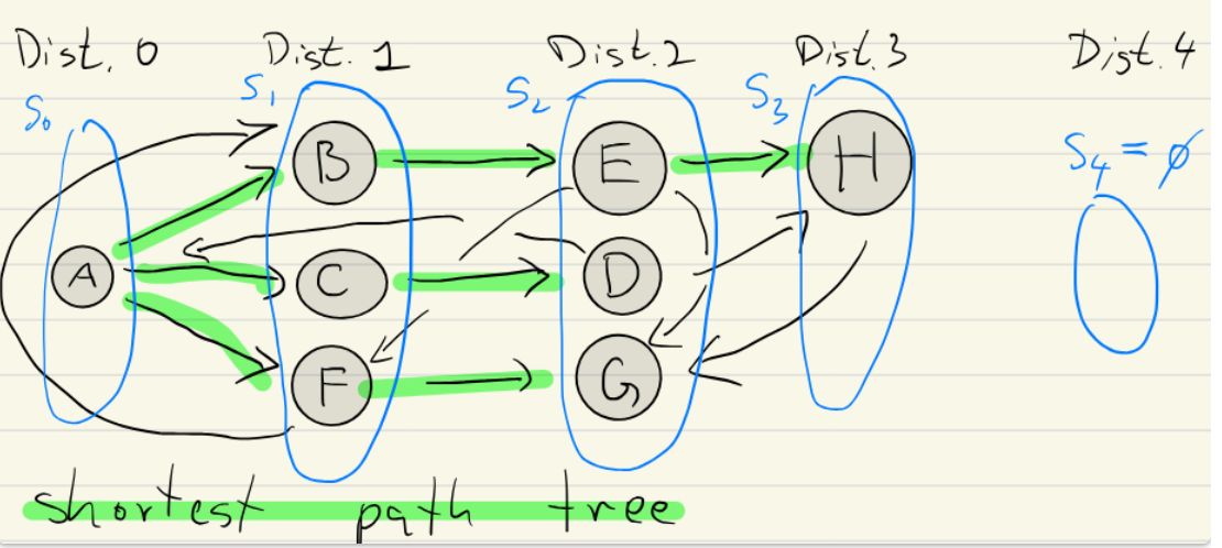
Current
Note has been deleted
Field-by-field Comparison
| Field | Before | After |
|---|---|---|
| Front | ||
| Back |
Note 258: ETH::1. Semester::A&D
Deck: ETH::1. Semester::A&D
Note Type: Algorithms
GUID:
deleted
Note Type: Algorithms
GUID:
rUd4]Y&$Fr
Deleted Note
Front
Runtime of Maximum Subarray Sum?
Back
Runtime of Maximum Subarray Sum?
\(\Theta(n)\)
Current
Note has been deleted
Field-by-field Comparison
| Field | Before | After |
|---|---|---|
| Name | ||
| Runtime | ||
| Approach | ||
| Pseudocode |
Note 259: ETH::1. Semester::A&D
Deck: ETH::1. Semester::A&D
Note Type: Horvath Classic
GUID:
deleted
Note Type: Horvath Classic
GUID:
ra?I5x|G>*
Deleted Note
Front
Runtime of operations in an adjacency matrix?
Back
Runtime of operations in an adjacency matrix?
1. Check if \(uv \in E\): \(O(1)\)
2. Vertex \(u\) , find all adjacent vertices in: \(O(n)\)
2. Vertex \(u\) , find all adjacent vertices in: \(O(n)\)
Current
Note has been deleted
Field-by-field Comparison
| Field | Before | After |
|---|---|---|
| Front | ||
| Back |
Note 260: ETH::1. Semester::A&D
Deck: ETH::1. Semester::A&D
Note Type: Horvath Cloze
GUID:
deleted
Note Type: Horvath Cloze
GUID:
rnACRB4[8n
Deleted Note
Front
Pre-/Post-Ordering Classification for an edge \((u, v)\):
\(\text{pre}(v) < \text{pre}(u) < \text{post}(u) < \text{post}(v)\): back edge
\(\text{pre}(v) < \text{pre}(u) < \text{post}(u) < \text{post}(v)\): back edge
Back
Pre-/Post-Ordering Classification for an edge \((u, v)\):
\(\text{pre}(v) < \text{pre}(u) < \text{post}(u) < \text{post}(v)\): back edge
\(\text{pre}(v) < \text{pre}(u) < \text{post}(u) < \text{post}(v)\): back edge
exists a cycle!
Current
Note has been deleted
Field-by-field Comparison
| Field | Before | After |
|---|---|---|
| Text | ||
| Extra |
Note 261: ETH::1. Semester::A&D
Deck: ETH::1. Semester::A&D
Note Type: Horvath Cloze
GUID:
deleted
Note Type: Horvath Cloze
GUID:
rp1#iPsvnq
Deleted Note
Front
In a linked list, the keys don't appear in order in memory. They each contain a pointer to the next element in the list instead.
We also have an extra pointer to the end.
We also have an extra pointer to the end.
Back
In a linked list, the keys don't appear in order in memory. They each contain a pointer to the next element in the list instead.
We also have an extra pointer to the end.
We also have an extra pointer to the end.
The last pointer of the list is a null pointer to indicate the end.
Current
Note has been deleted
Field-by-field Comparison
| Field | Before | After |
|---|---|---|
| Text | ||
| Extra |
Note 262: ETH::1. Semester::A&D
Deck: ETH::1. Semester::A&D
Note Type: Horvath Classic
GUID:
deleted
Note Type: Horvath Classic
GUID:
ruU|XgSe,e
Deleted Note
Front
What extra pointer does the ADT List store?
Back
What extra pointer does the ADT List store?
It stores an extra pointer to the end of the list (in a LinkedList to the last node, in an array to delimit the last element).
Current
Note has been deleted
Field-by-field Comparison
| Field | Before | After |
|---|---|---|
| Front | ||
| Back |
Note 263: ETH::1. Semester::A&D
Deck: ETH::1. Semester::A&D
Note Type: Horvath Classic
GUID:
deleted
Note Type: Horvath Classic
GUID:
rx?y6g[CSG
Deleted Note
Front
Describe the steps in BFS:
Back
Describe the steps in BFS:
BFS is a shortest path algorithm.
- Initialisation:
- Set the distance to all vertices to \(\infty\) in the
d[v]array. Set thed[s] = 0. - Initialise a Queue \(Q\) with \(s\)
- Set the dictionary
parent = {}
- Set the distance to all vertices to \(\infty\) in the
- Exploration:
- Dequeue the first element in the queue $v$
- For all adjacent nodes \(u\) with distance \(= \infty\) (not visited yet):
- Set the distance
d[u] = d[v] + 1 - add \(u\) to the queue
- Set the
parent[u] = v.
- Set the distance
- Return: We return the distances and the shortest path tree
The queue ensures that we don't mix up the order.
Current
Note has been deleted
Field-by-field Comparison
| Field | Before | After |
|---|---|---|
| Front | ||
| Back |
Note 264: ETH::1. Semester::A&D
Deck: ETH::1. Semester::A&D
Note Type: Horvath Cloze
GUID:
deleted
Note Type: Horvath Cloze
GUID:
rzX#2=8CU?
Deleted Note
Front
In graph theory, a cycle (Kreis) is a closed walk without repeated vertices and at least three vertices.
Back
In graph theory, a cycle (Kreis) is a closed walk without repeated vertices and at least three vertices.
Current
Note has been deleted
Field-by-field Comparison
| Field | Before | After |
|---|---|---|
| Text |
Note 265: ETH::1. Semester::A&D
Deck: ETH::1. Semester::A&D
Note Type: Horvath Cloze
GUID:
deleted
Note Type: Horvath Cloze
GUID:
s++QypVica
Deleted Note
Front
A PriorityQueue is like a queue, with the difference that every key is associated with a natural number which indicates the importance.
Back
A PriorityQueue is like a queue, with the difference that every key is associated with a natural number which indicates the importance.
The elements are then returned in the order of this importance.
Current
Note has been deleted
Field-by-field Comparison
| Field | Before | After |
|---|---|---|
| Text | ||
| Extra |
Note 266: ETH::1. Semester::A&D
Deck: ETH::1. Semester::A&D
Note Type: Horvath Cloze
GUID:
deleted
Note Type: Horvath Cloze
GUID:
s0knxb/
Deleted Note
Front
The height \(h(v)\) in Johnson's Algorithm is always negative \(\leq 0\).
Back
The height \(h(v)\) in Johnson's Algorithm is always negative \(\leq 0\).
Current
Note has been deleted
Field-by-field Comparison
| Field | Before | After |
|---|---|---|
| Text |
Note 267: ETH::1. Semester::A&D
Deck: ETH::1. Semester::A&D
Note Type: Horvath Cloze
GUID:
deleted
Note Type: Horvath Cloze
GUID:
s6a5!K0P)L
Deleted Note
Front
| Operation | Array | Singly Linked List | Doubly Linked List |
|---|---|---|---|
insert(k,L) |
\(O(1)\) | \(O(1)\) | \(O(1)\) |
get(i,L) |
\(O(1)\) | \(O(l)\) | \(O(j)\) |
insertAfter(k,k',L) |
\(O(l)\) | \(O(1)\) | \(O(1)\) |
delete(k,L) |
\(O(l)\) | \(O(l)\) | \(O(1)\) |
We assume to have a pointer to the end of the list here. |
Back
| Operation | Array | Singly Linked List | Doubly Linked List |
|---|---|---|---|
insert(k,L) |
\(O(1)\) | \(O(1)\) | \(O(1)\) |
get(i,L) |
\(O(1)\) | \(O(l)\) | \(O(j)\) |
insertAfter(k,k',L) |
\(O(l)\) | \(O(1)\) | \(O(1)\) |
delete(k,L) |
\(O(l)\) | \(O(l)\) | \(O(1)\) |
We assume to have a pointer to the end of the list here. |
Current
Note has been deleted
Field-by-field Comparison
| Field | Before | After |
|---|---|---|
| Text |
Note 268: ETH::1. Semester::A&D
Deck: ETH::1. Semester::A&D
Note Type: Horvath Cloze
GUID:
deleted
Note Type: Horvath Cloze
GUID:
s@rY_v*&u_
Deleted Note
Front
A graph is bipartite if and only if it does not contain any cycles of odd length.
Back
A graph is bipartite if and only if it does not contain any cycles of odd length.
Current
Note has been deleted
Field-by-field Comparison
| Field | Before | After |
|---|---|---|
| Text |
Note 269: ETH::1. Semester::A&D
Deck: ETH::1. Semester::A&D
Note Type: Horvath Classic
GUID:
deleted
Note Type: Horvath Classic
GUID:
sPqRN2wuHY
Deleted Note
Front
How does Depth-first-search work and what is its runtime for the two implementations of a graph?
Back
How does Depth-first-search work and what is its runtime for the two implementations of a graph?
a depth first search marks the vertices it visits, at each vertex it looks for a vertex it has not yet visited and if there are none, it tracks back to a vertex which still has some unvisited adjacent nodes
its runtime in an adjacency matrix is \(O(n^2)\) as it has to visit each vertex once and search through all \(n\) potential neighbors
implemented using adjacency lists, the runtime is \(O(n+m)\) as we still have to visit each vertex once but we only have to search through at most \(\text{deg}_{out}(u)\) vertices at each step, which adds up to searching through all the edges
Current
Note has been deleted
Field-by-field Comparison
| Field | Before | After |
|---|---|---|
| Front | ||
| Back |
Note 270: ETH::1. Semester::A&D
Deck: ETH::1. Semester::A&D
Note Type: Horvath Classic
GUID:
deleted
Note Type: Horvath Classic
GUID:
sS2;w|7M-!
Deleted Note
Front
What condition on the function \(T\) does the Master Theorem set?
Back
What condition on the function \(T\) does the Master Theorem set?
It only holds if \(n = 2^k\) or the function is increasing.
Current
Note has been deleted
Field-by-field Comparison
| Field | Before | After |
|---|---|---|
| Front | ||
| Back |
Note 271: ETH::1. Semester::A&D
Deck: ETH::1. Semester::A&D
Note Type: Horvath Cloze
GUID:
deleted
Note Type: Horvath Cloze
GUID:
sap]uaOK!q
Deleted Note
Front
Choose a tight bound!
\(O(n^k) \leq O(k^n)\)
\(O(n^k) \leq O(k^n)\)
Back
Choose a tight bound!
\(O(n^k) \leq O(k^n)\)
\(O(n^k) \leq O(k^n)\)
Current
Note has been deleted
Field-by-field Comparison
| Field | Before | After |
|---|---|---|
| Text |
Note 272: ETH::1. Semester::A&D
Deck: ETH::1. Semester::A&D
Note Type: Horvath Cloze
GUID:
deleted
Note Type: Horvath Cloze
GUID:
t/(N7FzdP}
Deleted Note
Front
The ADT priorityQueue can be efficiently implemented using a MaxHeap. This guarantees \(O(\log n)\) for both operations.
Back
The ADT priorityQueue can be efficiently implemented using a MaxHeap. This guarantees \(O(\log n)\) for both operations.
Current
Note has been deleted
Field-by-field Comparison
| Field | Before | After |
|---|---|---|
| Text |
Note 273: ETH::1. Semester::A&D
Deck: ETH::1. Semester::A&D
Note Type: Algorithms
GUID:
deleted
Note Type: Algorithms
GUID:
t:15}v~LmN
Deleted Note
Front
Runtime of Bellman-Ford?
Back
Runtime of Bellman-Ford?
\(O(|V| \cdot |E|)\) (uses DP)
We iterate over all edges in the "relaxation" thus the time complexity of that step is \(O(m)\) (the actual check is \(O(1)\)).
As we relax \(n - 1\) (or \(n\) for negative cycle check) times, the total runtime is \(O(n \cdot m)\).
We iterate over all edges in the "relaxation" thus the time complexity of that step is \(O(m)\) (the actual check is \(O(1)\)).
As we relax \(n - 1\) (or \(n\) for negative cycle check) times, the total runtime is \(O(n \cdot m)\).
Current
Note has been deleted
Field-by-field Comparison
| Field | Before | After |
|---|---|---|
| Name | ||
| Runtime | ||
| Requirements | ||
| Approach | ||
| Pseudocode | ||
| Use Case |
Note 274: ETH::1. Semester::A&D
Deck: ETH::1. Semester::A&D
Note Type: Horvath Classic
GUID:
deleted
Note Type: Horvath Classic
GUID:
tH)JXa7KfA
Deleted Note
Front
Worst case for search in a binary tree?
Back
Worst case for search in a binary tree?
Binary trees are not necessarily balanced, hence it is possible that \(h >> \log_2 n\).
Worst case example if inserted in ascending order:
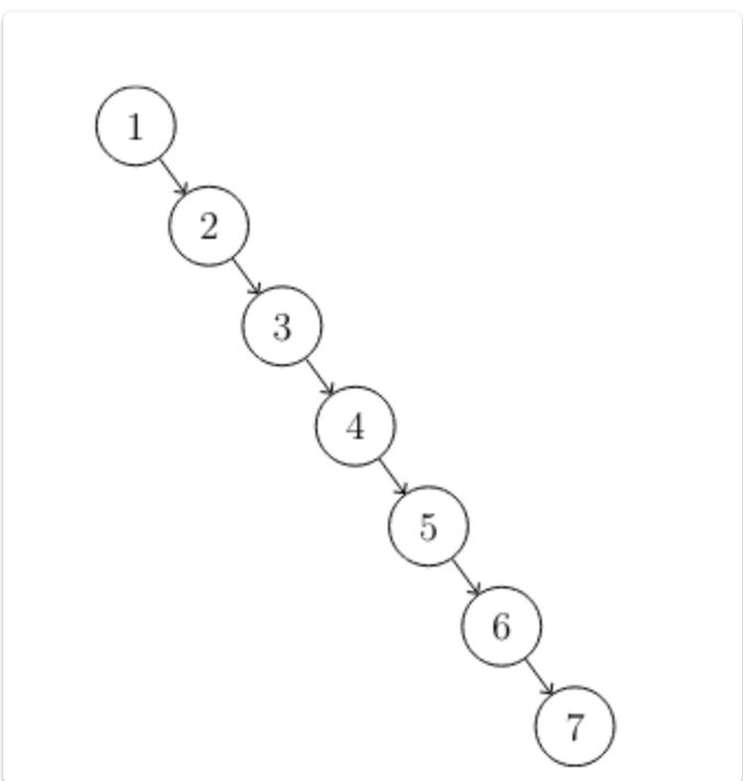
Worst case example if inserted in ascending order:
Current
Note has been deleted
Field-by-field Comparison
| Field | Before | After |
|---|---|---|
| Front | ||
| Back |
Note 275: ETH::1. Semester::A&D
Deck: ETH::1. Semester::A&D
Note Type: Algorithms
GUID:
deleted
Note Type: Algorithms
GUID:
tYh57HT9#t
Deleted Note
Front
Runtime of Jump Game?
Back
Runtime of Jump Game?
\(O(n)\) (hyper-optimised version)
Current
Note has been deleted
Field-by-field Comparison
| Field | Before | After |
|---|---|---|
| Name | ||
| Runtime | ||
| Requirements | ||
| Pseudocode |
Note 276: ETH::1. Semester::A&D
Deck: ETH::1. Semester::A&D
Note Type: Horvath Cloze
GUID:
deleted
Note Type: Horvath Cloze
GUID:
t]QH{.^=tP
Deleted Note
Front
The Karatsuba algorithm provides an asymptotically faster way to multiply numbers.
Back
The Karatsuba algorithm provides an asymptotically faster way to multiply numbers.
Current
Note has been deleted
Field-by-field Comparison
| Field | Before | After |
|---|---|---|
| Text |
Note 277: ETH::1. Semester::A&D
Deck: ETH::1. Semester::A&D
Note Type: Algorithms
GUID:
deleted
Note Type: Algorithms
GUID:
u%cN;v|jjQ
Deleted Note
Front
Back
Runtime of
BFS
Runtime: {{c1::\( \mathcal{O}(|E| + |V|) \)}}
Approach:
Uses:
?Current
Note has been deleted
Field-by-field Comparison
| Field | Before | After |
|---|---|---|
| Name |
Note 278: ETH::1. Semester::A&D
Deck: ETH::1. Semester::A&D
Note Type: Horvath Cloze
GUID:
deleted
Note Type: Horvath Cloze
GUID:
u)lmsqp*H!
Deleted Note
Front
A stack is also called a LIFO queue.
Back
A stack is also called a LIFO queue.
Current
Note has been deleted
Field-by-field Comparison
| Field | Before | After |
|---|---|---|
| Text |
Note 279: ETH::1. Semester::A&D
Deck: ETH::1. Semester::A&D
Note Type: Horvath Cloze
GUID:
deleted
Note Type: Horvath Cloze
GUID:
u2lDE>&5/e
Deleted Note
Front
{{c1:: \(\sum_{j = 1}^{n} \sum_{k = \textbf{j} }^{n} 1\)::Sum}} \(=\) {{c2:: \(\sum_{j = 1}^n (n - j + 1) = \frac{n(n + 1)}{2}\) }}
Back
{{c1:: \(\sum_{j = 1}^{n} \sum_{k = \textbf{j} }^{n} 1\)::Sum}} \(=\) {{c2:: \(\sum_{j = 1}^n (n - j + 1) = \frac{n(n + 1)}{2}\) }}
inner loop depends on outer
Current
Note has been deleted
Field-by-field Comparison
| Field | Before | After |
|---|---|---|
| Text | ||
| Extra |
Note 280: ETH::1. Semester::A&D
Deck: ETH::1. Semester::A&D
Note Type: Horvath Classic
GUID:
deleted
Note Type: Horvath Classic
GUID:
uHC]1fZd$=
Deleted Note
Front
What is the tree condition for 2-3 Trees implementing a dictionary?
Back
What is the tree condition for 2-3 Trees implementing a dictionary?
Each node has 2 or 3 children and all leaves are on the same level.
Current
Note has been deleted
Field-by-field Comparison
| Field | Before | After |
|---|---|---|
| Front | ||
| Back |
Note 281: ETH::1. Semester::A&D
Deck: ETH::1. Semester::A&D
Note Type: Horvath Cloze
GUID:
deleted
Note Type: Horvath Cloze
GUID:
ub(U6EB=d{
Deleted Note
Front
A topological ordering of vertices is an order such that for every edge \((u, v) \), \(u\) comes before \(v\).
Back
A topological ordering of vertices is an order such that for every edge \((u, v) \), \(u\) comes before \(v\).
thus all arrows point rightwards.
Current
Note has been deleted
Field-by-field Comparison
| Field | Before | After |
|---|---|---|
| Text | ||
| Extra |
Note 282: ETH::1. Semester::A&D
Deck: ETH::1. Semester::A&D
Note Type: Horvath Cloze
GUID:
deleted
Note Type: Horvath Cloze
GUID:
uxhT]f%32k
Deleted Note
Front
Master Theorem: If \(b = \log_2(a)\) then {{c2:: \(T(n) \leq O(n^{\log_2 a} \cdot \log n)\)}}.
Back
Master Theorem: If \(b = \log_2(a)\) then {{c2:: \(T(n) \leq O(n^{\log_2 a} \cdot \log n)\)}}.
The recursive and non-recursive work is balanced.
Current
Note has been deleted
Field-by-field Comparison
| Field | Before | After |
|---|---|---|
| Text | ||
| Extra |
Note 283: ETH::1. Semester::A&D
Deck: ETH::1. Semester::A&D
Note Type: Horvath Classic
GUID:
deleted
Note Type: Horvath Classic
GUID:
v%fJG/oUBR
Deleted Note
Front
How many edges does a tree with \(n\) vertices have?
Back
How many edges does a tree with \(n\) vertices have?
\(n-1\) edges
Current
Note has been deleted
Field-by-field Comparison
| Field | Before | After |
|---|---|---|
| Front | ||
| Back |
Note 284: ETH::1. Semester::A&D
Deck: ETH::1. Semester::A&D
Note Type: Horvath Classic
GUID:
deleted
Note Type: Horvath Classic
GUID:
v,>nr{ym:e
Deleted Note
Front
What is an ADT?
Back
What is an ADT?
An abstract data type describes a wishlist for operations we want to perform on our data.
Current
Note has been deleted
Field-by-field Comparison
| Field | Before | After |
|---|---|---|
| Front | ||
| Back |
Note 285: ETH::1. Semester::A&D
Deck: ETH::1. Semester::A&D
Note Type: Horvath Classic
GUID:
deleted
Note Type: Horvath Classic
GUID:
v7@jgp_hjT
Deleted Note
Front
How can we find a cross edge via DFS?
Back
How can we find a cross edge via DFS?
If we find vertex with both pre- and post-values set, there's a cross edge.
Current
Note has been deleted
Field-by-field Comparison
| Field | Before | After |
|---|---|---|
| Front | ||
| Back |
Note 286: ETH::1. Semester::A&D
Deck: ETH::1. Semester::A&D
Note Type: Horvath Classic
GUID:
deleted
Note Type: Horvath Classic
GUID:
vE[;wMoI5.
Deleted Note
Front
What is the optimal substructure property of shortest paths?
Back
What is the optimal substructure property of shortest paths?
Any subpath of a shortest path is itself the shortest path between its endpoints (requires no negative cycles).
Current
Note has been deleted
Field-by-field Comparison
| Field | Before | After |
|---|---|---|
| Front | ||
| Back |
Note 287: ETH::1. Semester::A&D
Deck: ETH::1. Semester::A&D
Note Type: Horvath Classic
GUID:
deleted
Note Type: Horvath Classic
GUID:
vQJH81Jg-1
Deleted Note
Front
For \(T(n) = 4T(n/2) + n\), which Master Theorem case applies?
Back
For \(T(n) = 4T(n/2) + n\), which Master Theorem case applies?
Because \(b = 1\) and \(\log_2(a) = \log_2 4 = 2 > b\), therefore \(T(n) = \Theta(n^2)\).
Current
Note has been deleted
Field-by-field Comparison
| Field | Before | After |
|---|---|---|
| Front | ||
| Back |
Note 288: ETH::1. Semester::A&D
Deck: ETH::1. Semester::A&D
Note Type: Horvath Classic
GUID:
deleted
Note Type: Horvath Classic
GUID:
vSWG3t+7{<
Deleted Note
Front
\(e^{\ln c} =\) ?
Back
\(e^{\ln c} =\) ?
\(c\)
Current
Note has been deleted
Field-by-field Comparison
| Field | Before | After |
|---|---|---|
| Front | ||
| Back |
Note 289: ETH::1. Semester::A&D
Deck: ETH::1. Semester::A&D
Note Type: Horvath Cloze
GUID:
deleted
Note Type: Horvath Cloze
GUID:
vfw3/~)/(m
Deleted Note
Front
Master Theorem: If \(b > \log_2(a)\) then \(T(n) \leq O(n^b)\).
Back
Master Theorem: If \(b > \log_2(a)\) then \(T(n) \leq O(n^b)\).
This is the case for which the work outside the recursion dominates.
Current
Note has been deleted
Field-by-field Comparison
| Field | Before | After |
|---|---|---|
| Text | ||
| Extra |
Note 290: ETH::1. Semester::A&D
Deck: ETH::1. Semester::A&D
Note Type: Horvath Classic
GUID:
deleted
Note Type: Horvath Classic
GUID:
vgCb-fRsjm
Deleted Note
Front
How can we get the runtime of an algorithm based on it's DP table?
Back
How can we get the runtime of an algorithm based on it's DP table?
We use the number of entries * the time to compute them (usually \(O(1)\))
Current
Note has been deleted
Field-by-field Comparison
| Field | Before | After |
|---|---|---|
| Front | ||
| Back |
Note 291: ETH::1. Semester::A&D
Deck: ETH::1. Semester::A&D
Note Type: Horvath Classic
GUID:
deleted
Note Type: Horvath Classic
GUID:
v{-8tJEW)=
Deleted Note
Front
What is the length of a walk?
Back
What is the length of a walk?
The length of a walk \((v_0, v_1, \dots, v_k)\) is \(k\), i.e. the number of vertices minus 1.
A walk of length \(l\) connects \(l + 1\) vertices.
A walk of length \(l\) connects \(l + 1\) vertices.
Current
Note has been deleted
Field-by-field Comparison
| Field | Before | After |
|---|---|---|
| Front | ||
| Back |
Note 292: ETH::1. Semester::A&D
Deck: ETH::1. Semester::A&D
Note Type: Horvath Cloze
GUID:
deleted
Note Type: Horvath Cloze
GUID:
v|.y5zi[:;
Deleted Note
Front
Prim's Algorithm Invariants:
The distances "d[.] = " in the distance array are the values of the vertices in the priority queue (see line decrease_key(H, v, d[v])).
Back
Prim's Algorithm Invariants:
The distances "d[.] = " in the distance array are the values of the vertices in the priority queue (see line decrease_key(H, v, d[v])).
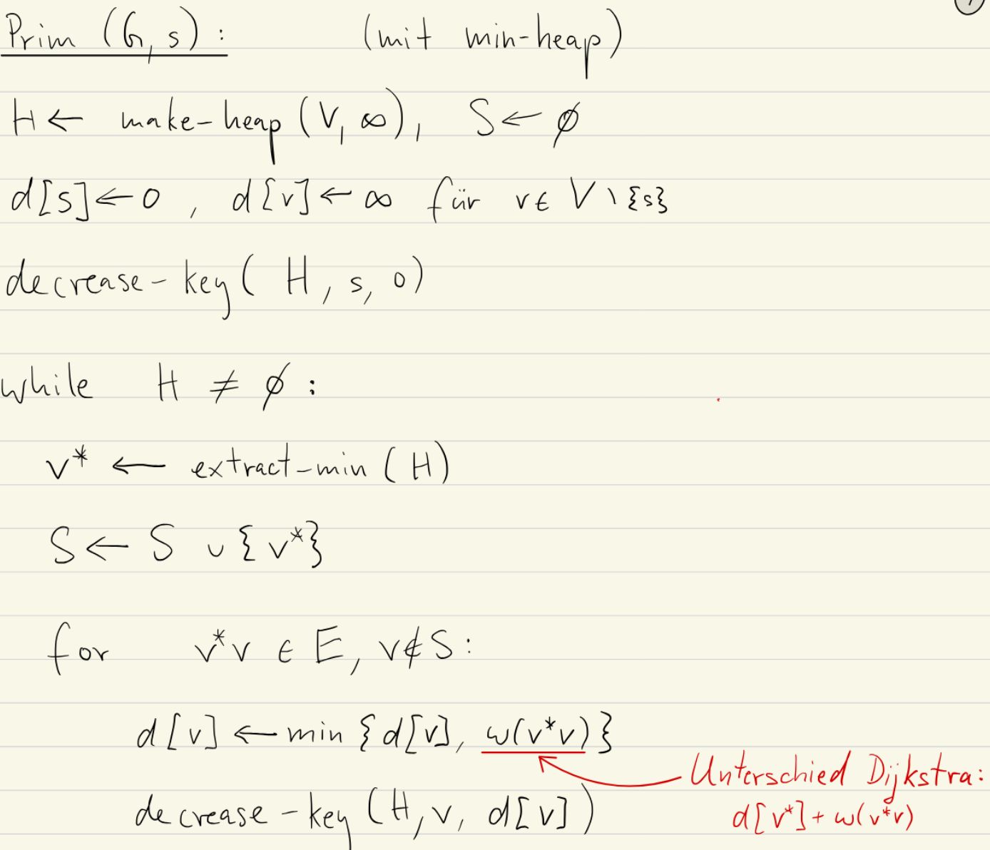
Current
Note has been deleted
Field-by-field Comparison
| Field | Before | After |
|---|---|---|
| Text | ||
| Extra |
Note 293: ETH::1. Semester::A&D
Deck: ETH::1. Semester::A&D
Note Type: Horvath Classic
GUID:
deleted
Note Type: Horvath Classic
GUID:
w2#a}f;^-i
Deleted Note
Front
How many leaf nodes can a 2-3 tree of depth \(h\) have?
Back
How many leaf nodes can a 2-3 tree of depth \(h\) have?
\(2^h \leq n \leq 3^h\) with \(n\) representing the number of leaf nodes.
Current
Note has been deleted
Field-by-field Comparison
| Field | Before | After |
|---|---|---|
| Front | ||
| Back |
Note 294: ETH::1. Semester::A&D
Deck: ETH::1. Semester::A&D
Note Type: Horvath Cloze
GUID:
deleted
Note Type: Horvath Cloze
GUID:
wD<:EQZU&2
Deleted Note
Front
Prim's Algorithm is similar to Dijkstra's with the difference that {{c1:: \(d[v] = \min \{d[v], w(v*, v)\}\) instead of \(d[v^*] + w(v^*, v)\) }}.
Back
Prim's Algorithm is similar to Dijkstra's with the difference that {{c1:: \(d[v] = \min \{d[v], w(v*, v)\}\) instead of \(d[v^*] + w(v^*, v)\) }}.
Dijkstra's find the shortest distance to each vertex, thus it tracks the total distance.
Prim's needs to build the MST. Since we add vertex \(v\) to the MST in the loop, we now want to know the new least distance to the MST for each node.
Prim's needs to build the MST. Since we add vertex \(v\) to the MST in the loop, we now want to know the new least distance to the MST for each node.
Current
Note has been deleted
Field-by-field Comparison
| Field | Before | After |
|---|---|---|
| Text | ||
| Extra |
Note 295: ETH::1. Semester::A&D
Deck: ETH::1. Semester::A&D
Note Type: Horvath Cloze
GUID:
deleted
Note Type: Horvath Cloze
GUID:
wStzO9J_2Q
Deleted Note
Front
If \(f \leq O(h)\) and \(g \leq O(h)\), then \(f + g \leq O(h)\).
Back
If \(f \leq O(h)\) and \(g \leq O(h)\), then \(f + g \leq O(h)\).
Current
Note has been deleted
Field-by-field Comparison
| Field | Before | After |
|---|---|---|
| Text |
Note 296: ETH::1. Semester::A&D
Deck: ETH::1. Semester::A&D
Note Type: Horvath Cloze
GUID:
deleted
Note Type: Horvath Cloze
GUID:
wbdb9#fK:J
Deleted Note
Front
The height of a 2-3 Tree for \(n\) keys is \(\leq \log_2(n)\) thus \(h={{c2::O(\log(n))::\textbf{O-notation} }}\).
Back
The height of a 2-3 Tree for \(n\) keys is \(\leq \log_2(n)\) thus \(h={{c2::O(\log(n))::\textbf{O-notation} }}\).
Note that for the case \(n = 1\) the root has one leaf with the key.
Current
Note has been deleted
Field-by-field Comparison
| Field | Before | After |
|---|---|---|
| Text | ||
| Extra |
Note 297: ETH::1. Semester::A&D
Deck: ETH::1. Semester::A&D
Note Type: Horvath Classic
GUID:
deleted
Note Type: Horvath Classic
GUID:
wxuX$c!)%k
Deleted Note
Front
A graph with this DP table from Floyd-Warshall:
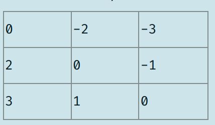
contains ___ negative cycles.
contains ___ negative cycles.
Back
A graph with this DP table from Floyd-Warshall:
contains ___ negative cycles.
contains ___ negative cycles.
no (there is no diagonal \(< 0\))
Current
Note has been deleted
Field-by-field Comparison
| Field | Before | After |
|---|---|---|
| Front | ||
| Back |
Note 298: ETH::1. Semester::A&D
Deck: ETH::1. Semester::A&D
Note Type: Horvath Classic
GUID:
deleted
Note Type: Horvath Classic
GUID:
w{Q]%!`f&#
Deleted Note
Front
How do we need to manipulate a graph in order to create a closed Eulerian walk from a normal Eulerian walk?
Back
How do we need to manipulate a graph in order to create a closed Eulerian walk from a normal Eulerian walk?
Add an edge connecting the end to the start point (both of which have odd degrees).
Current
Note has been deleted
Field-by-field Comparison
| Field | Before | After |
|---|---|---|
| Front | ||
| Back |
Note 299: ETH::1. Semester::A&D
Deck: ETH::1. Semester::A&D
Note Type: Horvath Cloze
GUID:
deleted
Note Type: Horvath Cloze
GUID:
w|i$)J%}4f
Deleted Note
Front
In graph theory, a Hamiltonian cycle (Hamiltonkreis) is a cycle that contains every vertex.
Back
In graph theory, a Hamiltonian cycle (Hamiltonkreis) is a cycle that contains every vertex.
Current
Note has been deleted
Field-by-field Comparison
| Field | Before | After |
|---|---|---|
| Text |
Note 300: ETH::1. Semester::A&D
Deck: ETH::1. Semester::A&D
Note Type: Horvath Cloze
GUID:
deleted
Note Type: Horvath Cloze
GUID:
x@F_EbzW}O
Deleted Note
Front
Prim's Algorithm Invariants:
The priority queue \(H = V \setminus S\) (\(V\) set of all vertices, \(S\) vertices currently in the MST) never contains a vertex already in the MST.
The priority queue \(H = V \setminus S\) (\(V\) set of all vertices, \(S\) vertices currently in the MST) never contains a vertex already in the MST.
Back
Prim's Algorithm Invariants:
The priority queue \(H = V \setminus S\) (\(V\) set of all vertices, \(S\) vertices currently in the MST) never contains a vertex already in the MST.
The priority queue \(H = V \setminus S\) (\(V\) set of all vertices, \(S\) vertices currently in the MST) never contains a vertex already in the MST.
Current
Note has been deleted
Field-by-field Comparison
| Field | Before | After |
|---|---|---|
| Text |
Note 301: ETH::1. Semester::A&D
Deck: ETH::1. Semester::A&D
Note Type: Horvath Cloze
GUID:
deleted
Note Type: Horvath Cloze
GUID:
xI`7oXbl[?
Deleted Note
Front
If \(\frac{f(n)}{g(n)}\) tends to {{c1::\(C \in \mathbb{R}^+\)}}, then \(f \leq O(g)\) and \(g \leq O(f) \Leftrightarrow f = \Theta(g)\).
Back
If \(\frac{f(n)}{g(n)}\) tends to {{c1::\(C \in \mathbb{R}^+\)}}, then \(f \leq O(g)\) and \(g \leq O(f) \Leftrightarrow f = \Theta(g)\).
Current
Note has been deleted
Field-by-field Comparison
| Field | Before | After |
|---|---|---|
| Text |
Note 302: ETH::1. Semester::A&D
Deck: ETH::1. Semester::A&D
Note Type: Horvath Classic
GUID:
deleted
Note Type: Horvath Classic
GUID:
xP1aIt[ejN
Deleted Note
Front
When \(f \geq \Omega(g)\), this means what exactly?
Back
When \(f \geq \Omega(g)\), this means what exactly?
\(\exists C \ge 0 \quad \forall n \in \mathbb{N} \quad f(n) \ge C\cdot g(n)\)
\(f\) grows asymptotically faster than \(g\)
\(f\) grows asymptotically faster than \(g\)
Current
Note has been deleted
Field-by-field Comparison
| Field | Before | After |
|---|---|---|
| Front | ||
| Back |
Note 303: ETH::1. Semester::A&D
Deck: ETH::1. Semester::A&D
Note Type: Horvath Cloze
GUID:
deleted
Note Type: Horvath Cloze
GUID:
xdGDHE`#zR
Deleted Note
Front
A datastructure is the implementation of the wishlist of operations defined in our ADT.
Back
A datastructure is the implementation of the wishlist of operations defined in our ADT.
Current
Note has been deleted
Field-by-field Comparison
| Field | Before | After |
|---|---|---|
| Text |
Note 304: ETH::1. Semester::A&D
Deck: ETH::1. Semester::A&D
Note Type: Horvath Classic
GUID:
deleted
Note Type: Horvath Classic
GUID:
x{57Az=}b`
Deleted Note
Front
How can we say that the function \(f\) and \(g\) grow asymptotically at the same rate?
Back
How can we say that the function \(f\) and \(g\) grow asymptotically at the same rate?
\(f = \Theta(g)\)
Current
Note has been deleted
Field-by-field Comparison
| Field | Before | After |
|---|---|---|
| Front | ||
| Back |
Note 305: ETH::1. Semester::A&D
Deck: ETH::1. Semester::A&D
Note Type: Horvath Classic
GUID:
deleted
Note Type: Horvath Classic
GUID:
y5w&L[iNjs
Deleted Note
Front
For \(T(n) = 2T(n/2) + n\), which Master Theorem case applies?
Back
For \(T(n) = 2T(n/2) + n\), which Master Theorem case applies?
Because \(b = 1\) and \(\log_2 a = \log_2 2 = 1 = b\), therefore \(T(n) = \Theta(n \log n)\).
Current
Note has been deleted
Field-by-field Comparison
| Field | Before | After |
|---|---|---|
| Front | ||
| Back |
Note 306: ETH::1. Semester::A&D
Deck: ETH::1. Semester::A&D
Note Type: Algorithms
GUID:
deleted
Note Type: Algorithms
GUID:
y@l`JCIJ<4
Deleted Note
Front
Runtime of BFS (Breadth First Search)?
Back
Runtime of BFS (Breadth First Search)?
\(O(|V|+|E|)\) (Adjacency List)
The runtime of BFS:
The runtime of BFS:
- each loop we take \(O(1 + \deg(u))\) time (go through the vertex \(u\)'s edges
- We loop a total of \(|V|\) times (we visit each edge max. 1 time)
Current
Note has been deleted
Field-by-field Comparison
| Field | Before | After |
|---|---|---|
| Name | ||
| Runtime | ||
| Requirements | ||
| Approach | ||
| Pseudocode | ||
| Use Case | ||
| Extra Info |
Note 307: ETH::1. Semester::A&D
Deck: ETH::1. Semester::A&D
Note Type: Horvath Cloze
GUID:
deleted
Note Type: Horvath Cloze
GUID:
yOa^MOZU`,
Deleted Note
Front
Choose a tight bound!
\(O(n) \leq O(\log(n!))\)
\(O(n) \leq O(\log(n!))\)
Back
Choose a tight bound!
\(O(n) \leq O(\log(n!))\)
\(O(n) \leq O(\log(n!))\)
Current
Note has been deleted
Field-by-field Comparison
| Field | Before | After |
|---|---|---|
| Text |
Note 308: ETH::1. Semester::A&D
Deck: ETH::1. Semester::A&D
Note Type: Horvath Cloze
GUID:
deleted
Note Type: Horvath Cloze
GUID:
yX`f0NZg((
Deleted Note
Front
The triangle inequality in a weighted graph is \(d(u, v) \leq d(u, w) + d(w, v)\).
Back
The triangle inequality in a weighted graph is \(d(u, v) \leq d(u, w) + d(w, v)\).
This holds, since if the path through \(w\) was actually cheaper, then \(d(u, v)\) would be wrong.
Does not hold in graphs with negative cycles.
Does not hold in graphs with negative cycles.
Current
Note has been deleted
Field-by-field Comparison
| Field | Before | After |
|---|---|---|
| Text | ||
| Extra |
Note 309: ETH::1. Semester::A&D
Deck: ETH::1. Semester::A&D
Note Type: Horvath Cloze
GUID:
deleted
Note Type: Horvath Cloze
GUID:
y_NK5>_:x4
Deleted Note
Front
In the edge \(e = \{u, v\}\), \(u\) and \(v\) are the endpoints of the edge.
Back
In the edge \(e = \{u, v\}\), \(u\) and \(v\) are the endpoints of the edge.
Current
Note has been deleted
Field-by-field Comparison
| Field | Before | After |
|---|---|---|
| Text |
Note 310: ETH::1. Semester::A&D
Deck: ETH::1. Semester::A&D
Note Type: Horvath Cloze
GUID:
deleted
Note Type: Horvath Cloze
GUID:
yg-tkTB|,7
Deleted Note
Front
{{c1:: \(\sum_{i = 1}^{n} i\log(i)\)}} \(\leq\) {{c2::\(\sum_{i = 1}^n n \log(n) = n^2 \log n\)::Sum}}
Back
{{c1:: \(\sum_{i = 1}^{n} i\log(i)\)}} \(\leq\) {{c2::\(\sum_{i = 1}^n n \log(n) = n^2 \log n\)::Sum}}
Current
Note has been deleted
Field-by-field Comparison
| Field | Before | After |
|---|---|---|
| Text |
Note 311: ETH::1. Semester::A&D
Deck: ETH::1. Semester::A&D
Note Type: Horvath Cloze
GUID:
deleted
Note Type: Horvath Cloze
GUID:
yy3TxuBe~r
Deleted Note
Front
A queue is also called FIFO.
Back
A queue is also called FIFO.
Current
Note has been deleted
Field-by-field Comparison
| Field | Before | After |
|---|---|---|
| Text |
Note 312: ETH::1. Semester::A&D
Deck: ETH::1. Semester::A&D
Note Type: Horvath Cloze
GUID:
deleted
Note Type: Horvath Cloze
GUID:
z4Nw/I#?J^
Deleted Note
Front
In graph theory, a path (Pfad) is a walk in which all vertices are distinct.
Back
In graph theory, a path (Pfad) is a walk in which all vertices are distinct.
Current
Note has been deleted
Field-by-field Comparison
| Field | Before | After |
|---|---|---|
| Text |
Note 313: ETH::1. Semester::A&D
Deck: ETH::1. Semester::A&D
Note Type: Horvath Classic
GUID:
deleted
Note Type: Horvath Classic
GUID:
z=SLl>>F5y
Deleted Note
Front
Simplify \(a^{log_b(n)} = \)
Back
Simplify \(a^{log_b(n)} = \)
\(n^{log_b(a)}\)
Current
Note has been deleted
Field-by-field Comparison
| Field | Before | After |
|---|---|---|
| Front | ||
| Back |
Note 314: ETH::1. Semester::A&D
Deck: ETH::1. Semester::A&D
Note Type: Horvath Cloze
GUID:
deleted
Note Type: Horvath Cloze
GUID:
zBLkhwqevO
Deleted Note
Front
Choose a tight bound!
\(O(n \log(n)) \leq O(n^k)\)
\(O(n \log(n)) \leq O(n^k)\)
Back
Choose a tight bound!
\(O(n \log(n)) \leq O(n^k)\)
\(O(n \log(n)) \leq O(n^k)\)
Current
Note has been deleted
Field-by-field Comparison
| Field | Before | After |
|---|---|---|
| Text |
Note 315: ETH::1. Semester::A&D
Deck: ETH::1. Semester::A&D
Note Type: Horvath Cloze
GUID:
deleted
Note Type: Horvath Cloze
GUID:
zjEd=>WPZ?
Deleted Note
Front
The number of distinct paths in a complete graph grows \(O(n!)\).
Back
The number of distinct paths in a complete graph grows \(O(n!)\).
Current
Note has been deleted
Field-by-field Comparison
| Field | Before | After |
|---|---|---|
| Text |
Note 316: ETH::1. Semester::A&D
Deck: ETH::1. Semester::A&D
Note Type: Algorithms
GUID:
deleted
Note Type: Algorithms
GUID:
z{8WPibSbC
Deleted Note
Front
Runtime of Dijkstra's Algorithm?
Back
Runtime of Dijkstra's Algorithm?
\(O((|V| + |E|) \log |V|)\) (or \(O(|V|^2)\)
The runtime is calculated from \(O(n + (\#\text{extract-min} + \#\text{decrease-key}) \cdot \log n)\) which gives \(O((n + m) \cdot \log n)\).
The runtime is calculated from \(O(n + (\#\text{extract-min} + \#\text{decrease-key}) \cdot \log n)\) which gives \(O((n + m) \cdot \log n)\).
Current
Note has been deleted
Field-by-field Comparison
| Field | Before | After |
|---|---|---|
| Name | ||
| Runtime | ||
| Requirements | ||
| Approach | ||
| Pseudocode | ||
| Use Case |
Note 317: ETH::1. Semester::A&D
Deck: ETH::1. Semester::A&D
Note Type: Horvath Cloze
GUID:
deleted
Note Type: Horvath Cloze
GUID:
|%{-v*KE>
Deleted Note
Front
The standard notation for \(|V|\) is \(n\) and for \(|E|\) is \(m\).
Back
The standard notation for \(|V|\) is \(n\) and for \(|E|\) is \(m\).
Current
Note has been deleted
Field-by-field Comparison
| Field | Before | After |
|---|---|---|
| Text |
Note 318: ETH::1. Semester::DiskMat
Deck: ETH::1. Semester::DiskMat
Note Type: Horvath Cloze
GUID:
deleted
Note Type: Horvath Cloze
GUID:
%-v5b-!x=
Deleted Note
Front
\( \neg (A \lor B) \) \( \equiv \) \( \neg A \land \neg B\)
Back
\( \neg (A \lor B) \) \( \equiv \) \( \neg A \land \neg B\)
de Morgan rules
Current
Note has been deleted
Field-by-field Comparison
| Field | Before | After |
|---|---|---|
| Text | ||
| Extra |
Note 319: ETH::1. Semester::DiskMat
Deck: ETH::1. Semester::DiskMat
Note Type: Horvath Cloze
GUID:
deleted
Note Type: Horvath Cloze
GUID:
.@%aS+kuV
Deleted Note
Front
In any ring \(\langle R; +, -, 0, \cdot, 1 \rangle\), and for all \(a, b \in R\) \(a0 =\) \(0a = 0\).
Back
In any ring \(\langle R; +, -, 0, \cdot, 1 \rangle\), and for all \(a, b \in R\) \(a0 =\) \(0a = 0\).
The zero (neutral of additive group) pulls all other elements to 0 by multiplication.
\(0a=(0-0)a=0a-0a=0\)
\(0a=(0-0)a=0a-0a=0\)
Current
Note has been deleted
Field-by-field Comparison
| Field | Before | After |
|---|---|---|
| Text | ||
| Extra |
Note 320: ETH::1. Semester::DiskMat
Deck: ETH::1. Semester::DiskMat
Note Type: Horvath Classic
GUID:
deleted
Note Type: Horvath Classic
GUID:
.H2xW-FA|
Deleted Note
Front
Which of the following are countable: \(\mathbb{N}\), \(\mathbb{Z}\), \(\mathbb{Q}\), \(\mathbb{R}\), \(\{0,1\}^*\), \(\{0,1\}^{\infty}\)?
Back
Which of the following are countable: \(\mathbb{N}\), \(\mathbb{Z}\), \(\mathbb{Q}\), \(\mathbb{R}\), \(\{0,1\}^*\), \(\{0,1\}^{\infty}\)?
Countable: \(\mathbb{N}\), \(\mathbb{Z}\), \(\mathbb{Q}\), \(\{0,1\}^*\)
Uncountable: \(\mathbb{R}\), \(\{0,1\}^{\infty}\)
Current
Note has been deleted
Field-by-field Comparison
| Field | Before | After |
|---|---|---|
| Front | ||
| Back |
Note 321: ETH::1. Semester::DiskMat
Deck: ETH::1. Semester::DiskMat
Note Type: Horvath Cloze
GUID:
deleted
Note Type: Horvath Cloze
GUID:
.d,WRJq.}
Deleted Note
Front
A subset \(H \subseteq G\) of a group is called a subgroup if \(H\) is closed with respect to all operations (operation, neutral, inverse).
Back
A subset \(H \subseteq G\) of a group is called a subgroup if \(H\) is closed with respect to all operations (operation, neutral, inverse).
Current
Note has been deleted
Field-by-field Comparison
| Field | Before | After |
|---|---|---|
| Text |
Note 322: ETH::1. Semester::DiskMat
Deck: ETH::1. Semester::DiskMat
Note Type: Horvath Cloze
GUID:
deleted
Note Type: Horvath Cloze
GUID:
6o/GG^(~_
Deleted Note
Front
In a group, the left cancellation law states: \(a = b\) \(\Leftrightarrow\) \(ca = cb\).
Back
In a group, the left cancellation law states: \(a = b\) \(\Leftrightarrow\) \(ca = cb\).
Current
Note has been deleted
Field-by-field Comparison
| Field | Before | After |
|---|---|---|
| Text |
Note 323: ETH::1. Semester::DiskMat
Deck: ETH::1. Semester::DiskMat
Note Type: Horvath Classic
GUID:
deleted
Note Type: Horvath Classic
GUID:
A+Li^bwkLL
Deleted Note
Front
Is this a lattice?
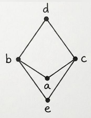
Back
Is this a lattice?
No, as \(\{b, c\}\) does not have a greatest lower bound. Both \(a\) and \(e\) would fit, but there isn't a greatest one.
Current
Note has been deleted
Field-by-field Comparison
| Field | Before | After |
|---|---|---|
| Front | ||
| Back |
Note 324: ETH::1. Semester::DiskMat
Deck: ETH::1. Semester::DiskMat
Note Type: Horvath Classic
GUID:
deleted
Note Type: Horvath Classic
GUID:
A0$~M#^-(C
Deleted Note
Front
If \(F \models G\) in predicate logic, what can we conclude via validity?
Back
If \(F \models G\) in predicate logic, what can we conclude via validity?
If \(F\) is valid, then \(G\) is also valid. (Logical consequence preserves validity)
Current
Note has been deleted
Field-by-field Comparison
| Field | Before | After |
|---|---|---|
| Front | ||
| Back |
Note 325: ETH::1. Semester::DiskMat
Deck: ETH::1. Semester::DiskMat
Note Type: Horvath Classic
GUID:
deleted
Note Type: Horvath Classic
GUID:
A9?srsv3Y:
Deleted Note
Front
What is the \((n, k)\)-error correcting code over the alphabet \(\mathcal{A}\) with \(|\mathcal{A}| = q\)?
Back
What is the \((n, k)\)-error correcting code over the alphabet \(\mathcal{A}\) with \(|\mathcal{A}| = q\)?
It's a subset of \(\mathcal{A}^n\) of cardinality \(q^k\).
Current
Note has been deleted
Field-by-field Comparison
| Field | Before | After |
|---|---|---|
| Front | ||
| Back |
Note 326: ETH::1. Semester::DiskMat
Deck: ETH::1. Semester::DiskMat
Note Type: Horvath Classic
GUID:
deleted
Note Type: Horvath Classic
GUID:
A>Qb$tT})[
Deleted Note
Front
Is the interval \([0, 1]\) countable or uncountable? What does this imply for \(\mathbb{R}\)?
Back
Is the interval \([0, 1]\) countable or uncountable? What does this imply for \(\mathbb{R}\)?
The interval is uncountable by Cantor's diagonal argument, thus \(\mathbb{R}\) is too.
Current
Note has been deleted
Field-by-field Comparison
| Field | Before | After |
|---|---|---|
| Front | ||
| Back |
Note 327: ETH::1. Semester::DiskMat
Deck: ETH::1. Semester::DiskMat
Note Type: Horvath Cloze
GUID:
deleted
Note Type: Horvath Cloze
GUID:
AFt:;I:*/e
Deleted Note
Front
\(a \mod m\) is the same as \(R_m(a)\)
Back
\(a \mod m\) is the same as \(R_m(a)\)
Current
Note has been deleted
Field-by-field Comparison
| Field | Before | After |
|---|---|---|
| Text |
Note 328: ETH::1. Semester::DiskMat
Deck: ETH::1. Semester::DiskMat
Note Type: Horvath Classic
GUID:
deleted
Note Type: Horvath Classic
GUID:
AOBg=yO4_)
Deleted Note
Front
Are the rational numbers \(\mathbb{Q}\) countable?
Back
Are the rational numbers \(\mathbb{Q}\) countable?
Yes, the rational numbers \(\mathbb{Q}\) are countable. They correspond to (a, b) tuples which can be mapped bijectively to the natural numbers.
Current
Note has been deleted
Field-by-field Comparison
| Field | Before | After |
|---|---|---|
| Front | ||
| Back |
Note 329: ETH::1. Semester::DiskMat
Deck: ETH::1. Semester::DiskMat
Note Type: Horvath Classic
GUID:
deleted
Note Type: Horvath Classic
GUID:
AR?8CyMux0
Deleted Note
Front
What is a polynomial over a commutative ring?
Back
What is a polynomial over a commutative ring?
A polynomial \(a(x)\) over a commutative ring \(R\) in the indeterminate \(x\) is a formal expression of the form: \[ a(x) = a_d x^d + a_{d-1}x^{d-1} + \cdots + a_1 x + a_0 = \sum_{i=0}^d a_i x^i \] for some non-negative integer \(d\), with \(a_i \in R\).
The set of polynomials in \(x\) over \(R\) is denoted \(R[x]\).
Current
Note has been deleted
Field-by-field Comparison
| Field | Before | After |
|---|---|---|
| Front | ||
| Back |
Note 330: ETH::1. Semester::DiskMat
Deck: ETH::1. Semester::DiskMat
Note Type: Horvath Cloze
GUID:
deleted
Note Type: Horvath Cloze
GUID:
Ak;RI/ADAm
Deleted Note
Front
To prove an isomorphism \(\phi: G \rightarrow H\), we need to prove:
- Well-definedness
- The image of \(\phi\) lies entirely within \(H\)
- The homomorphism-property \(\phi(g_1 \cdot g_2) = \phi(g_1) \cdot \phi(g_2)\) holds
- Injectivity
- Surjectivity
Back
To prove an isomorphism \(\phi: G \rightarrow H\), we need to prove:
- Well-definedness
- The image of \(\phi\) lies entirely within \(H\)
- The homomorphism-property \(\phi(g_1 \cdot g_2) = \phi(g_1) \cdot \phi(g_2)\) holds
- Injectivity
- Surjectivity
Current
Note has been deleted
Field-by-field Comparison
| Field | Before | After |
|---|---|---|
| Text |
Note 331: ETH::1. Semester::DiskMat
Deck: ETH::1. Semester::DiskMat
Note Type: Horvath Classic
GUID:
deleted
Note Type: Horvath Classic
GUID:
AluZ0L@#]a
Deleted Note
Front
What does it mean for a function \(f: A \to B\) to be injective?
Back
What does it mean for a function \(f: A \to B\) to be injective?
For \(a \neq a'\) we have \(f(a) \neq f(a')\).
No two distinct values are mapped to the same function value (no "collisions"). This is also called "one-to-one".
No two distinct values are mapped to the same function value (no "collisions"). This is also called "one-to-one".
Current
Note has been deleted
Field-by-field Comparison
| Field | Before | After |
|---|---|---|
| Front | ||
| Back |
Note 332: ETH::1. Semester::DiskMat
Deck: ETH::1. Semester::DiskMat
Note Type: Horvath Cloze
GUID:
deleted
Note Type: Horvath Cloze
GUID:
Am`UxH.Oyx
Deleted Note
Front
\(a \mid b\) means that {{c1::\(a\) divides \(b\), that is, there exists a \(c \in \mathbb{Z}\) such that \(b = ac\)}}
Back
\(a \mid b\) means that {{c1::\(a\) divides \(b\), that is, there exists a \(c \in \mathbb{Z}\) such that \(b = ac\)}}
\(\forall a \ne 0 \rightarrow a \mid 0\) and \(\forall a \quad 1 \mid a \land -1 \mid a\)
Current
Note has been deleted
Field-by-field Comparison
| Field | Before | After |
|---|---|---|
| Text | ||
| Extra |
Note 333: ETH::1. Semester::DiskMat
Deck: ETH::1. Semester::DiskMat
Note Type: Horvath Cloze
GUID:
deleted
Note Type: Horvath Cloze
GUID:
Amp7wwZ8FK
Deleted Note
Front
For a poset \((A;\preceq)\), two elements \(a,b\) are comparable if \(a \preceq b\) or \(b \preceq a\), otherwise they are incomparable.
Back
For a poset \((A;\preceq)\), two elements \(a,b\) are comparable if \(a \preceq b\) or \(b \preceq a\), otherwise they are incomparable.
Current
Note has been deleted
Field-by-field Comparison
| Field | Before | After |
|---|---|---|
| Text |
Note 334: ETH::1. Semester::DiskMat
Deck: ETH::1. Semester::DiskMat
Note Type: Horvath Cloze
GUID:
deleted
Note Type: Horvath Cloze
GUID:
Au5Kz9Rp2H
Deleted Note
Front
\(F\) \(\vdash\) \(F \lor G\) and \(F \vdash G \lor F\) are valid derivation rules.
Back
\(F\) \(\vdash\) \(F \lor G\) and \(F \vdash G \lor F\) are valid derivation rules.
Current
Note has been deleted
Field-by-field Comparison
| Field | Before | After |
|---|---|---|
| Text |
Note 335: ETH::1. Semester::DiskMat
Deck: ETH::1. Semester::DiskMat
Note Type: Horvath Classic
GUID:
deleted
Note Type: Horvath Classic
GUID:
Auz&g~bS8q
Deleted Note
Front
What is \(\lnot \forall x P(x)\) equivalent to?
Back
What is \(\lnot \forall x P(x)\) equivalent to?
\(\lnot \forall x P(x) \equiv \exists x \lnot P(x)\)
Current
Note has been deleted
Field-by-field Comparison
| Field | Before | After |
|---|---|---|
| Front | ||
| Back |
Note 336: ETH::1. Semester::DiskMat
Deck: ETH::1. Semester::DiskMat
Note Type: Horvath Cloze
GUID:
deleted
Note Type: Horvath Cloze
GUID:
Av3Ww9Kn5Y
Deleted Note
Front
For any \(i\) and \(k\), if \(t_1, \dots, t_k\) are terms, then {{c1::\(P_i^{(k)}(t_1, \dots, t_k)\) is a formula}}, called an atomic formula.
Back
For any \(i\) and \(k\), if \(t_1, \dots, t_k\) are terms, then {{c1::\(P_i^{(k)}(t_1, \dots, t_k)\) is a formula}}, called an atomic formula.
A formula in 1st order logic with no logical connectives (like \(\lnot, \land, \lor, \rightarrow \)) and no quantifiers (\(\forall, \exists\))
Current
Note has been deleted
Field-by-field Comparison
| Field | Before | After |
|---|---|---|
| Text | ||
| Extra |
Note 337: ETH::1. Semester::DiskMat
Deck: ETH::1. Semester::DiskMat
Note Type: Horvath Classic
GUID:
deleted
Note Type: Horvath Classic
GUID:
B)Cal)+#sy
Deleted Note
Front
What are De Morgan's laws?
Back
What are De Morgan's laws?
- \(\lnot(A \land B) \equiv \lnot A \lor \lnot B\)
- \(\lnot(A \lor B) \equiv \lnot A \land \lnot B\)
Current
Note has been deleted
Field-by-field Comparison
| Field | Before | After |
|---|---|---|
| Front | ||
| Back |
Note 338: ETH::1. Semester::DiskMat
Deck: ETH::1. Semester::DiskMat
Note Type: Horvath Cloze
GUID:
deleted
Note Type: Horvath Cloze
GUID:
B/hV
Deleted Note
Front
A poset \((A;\preceq)\) is well-ordered if it is totally ordered and every non-empty subset has a least element.
Back
A poset \((A;\preceq)\) is well-ordered if it is totally ordered and every non-empty subset has a least element.
Every totally ordered finite poset \(\rightarrow\) well-ordered
Infinite example: \((\mathbb{N}; \le)\)
Infinite counterexample \((\mathbb{Z}; \le)\)
Infinite counterexample \((\mathbb{Z}; \le)\)
Current
Note has been deleted
Field-by-field Comparison
| Field | Before | After |
|---|---|---|
| Text | ||
| Extra |
Note 339: ETH::1. Semester::DiskMat
Deck: ETH::1. Semester::DiskMat
Note Type: Horvath Cloze
GUID:
deleted
Note Type: Horvath Cloze
GUID:
B7%
Deleted Note
Front
Describe the RSA protocol:
- Alice generates primes \(p\) and \(q\)
- Set \(n = pq\) and \(f = \varphi(n) = (p - 1)(q - 1)\)
- {{c3:: Select \(e\): \(d \equiv_f e^{-1}\) the modular inverse (decryption)}}
- Send \(n\) and \(e\) to Bob
- {{c5:: Bob encrypts the plaintext \(m \in \{1, \dots, n -1 \}\) (unique modulo \(n\)) \(c = R_n(m^e)\) and sends it}}
- Alice decrypts using \(m = R_n(c^d)\)
Back
Describe the RSA protocol:
- Alice generates primes \(p\) and \(q\)
- Set \(n = pq\) and \(f = \varphi(n) = (p - 1)(q - 1)\)
- {{c3:: Select \(e\): \(d \equiv_f e^{-1}\) the modular inverse (decryption)}}
- Send \(n\) and \(e\) to Bob
- {{c5:: Bob encrypts the plaintext \(m \in \{1, \dots, n -1 \}\) (unique modulo \(n\)) \(c = R_n(m^e)\) and sends it}}
- Alice decrypts using \(m = R_n(c^d)\)
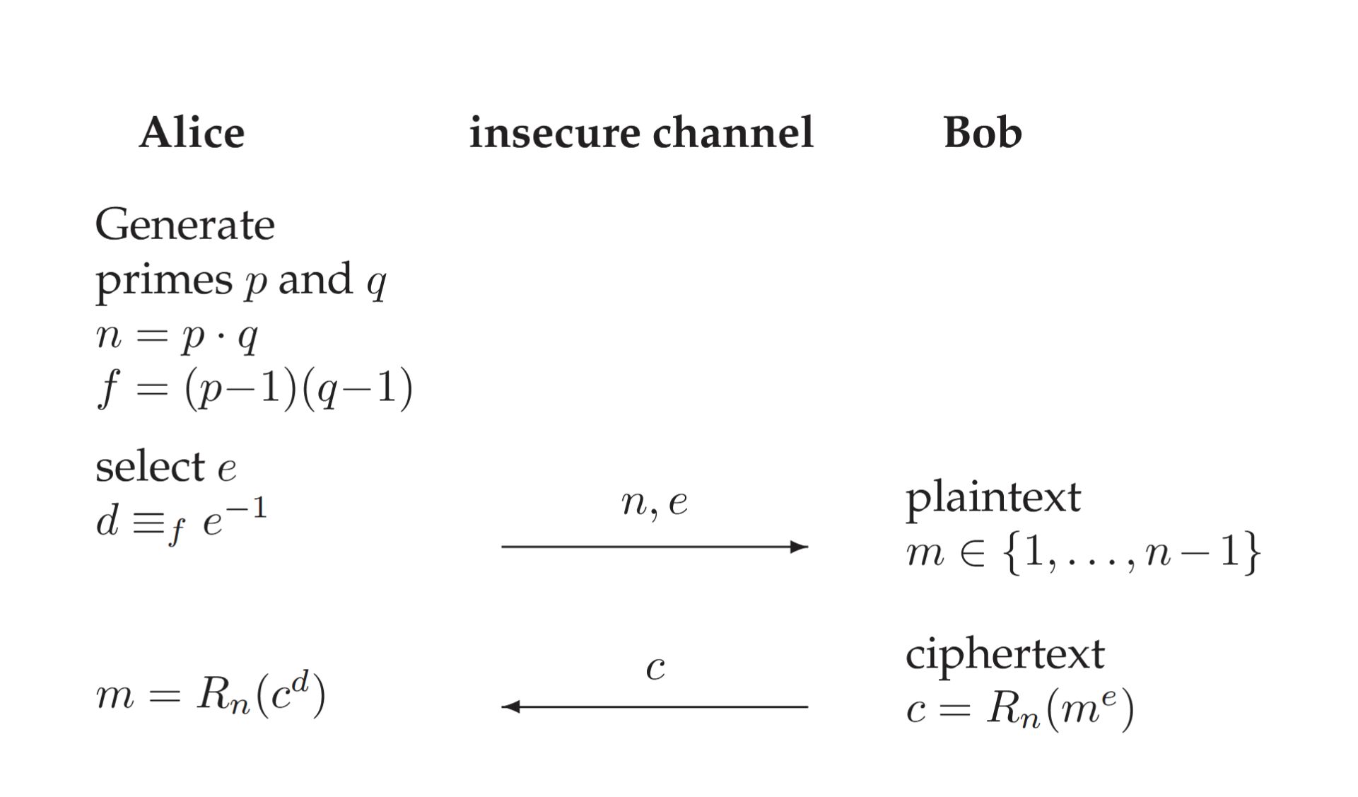
Current
Note has been deleted
Field-by-field Comparison
| Field | Before | After |
|---|---|---|
| Text | ||
| Extra |
Note 340: ETH::1. Semester::DiskMat
Deck: ETH::1. Semester::DiskMat
Note Type: Horvath Classic
GUID:
deleted
Note Type: Horvath Classic
GUID:
B7f%iVC#KH
Deleted Note
Front
What does it mean intuitively for two groups to be isomorphic?
Back
What does it mean intuitively for two groups to be isomorphic?
Two groups are isomorphic if they have the same structure - they "behave identically" even if they look different.
Analogy: Like two jigsaw puzzles that look completely different, but use the same cutout pattern. The same piece goes into the same place on both puzzles.
The bijection between them preserves all group operations and relationships.
Current
Note has been deleted
Field-by-field Comparison
| Field | Before | After |
|---|---|---|
| Front | ||
| Back |
Note 341: ETH::1. Semester::DiskMat
Deck: ETH::1. Semester::DiskMat
Note Type: Horvath Cloze
GUID:
deleted
Note Type: Horvath Cloze
GUID:
BA!Uj{h&4e
Deleted Note
Front
For a homomorphism \(h: G \rightarrow H\), the {{c1::image \(\text{Im} (h)\)}} is the set of all elements in \(H\) that are mapped to by some element in \(G\).
Back
For a homomorphism \(h: G \rightarrow H\), the {{c1::image \(\text{Im} (h)\)}} is the set of all elements in \(H\) that are mapped to by some element in \(G\).
Current
Note has been deleted
Field-by-field Comparison
| Field | Before | After |
|---|---|---|
| Text |
Note 342: ETH::1. Semester::DiskMat
Deck: ETH::1. Semester::DiskMat
Note Type: Horvath Classic
GUID:
deleted
Note Type: Horvath Classic
GUID:
BCPARdin7?
Deleted Note
Front
What is the logical principle behind case distinction?
Back
What is the logical principle behind case distinction?
For every \(k\) we have:
\[(A_1 \lor \dots \lor A_k) \land (A_1 \rightarrow B) \land \dots \land (A_k \rightarrow B) \models B\]
(If at least one case occurs, and all cases imply \(B\), then \(B\) holds)
(If at least one case occurs, and all cases imply \(B\), then \(B\) holds)
Current
Note has been deleted
Field-by-field Comparison
| Field | Before | After |
|---|---|---|
| Front | ||
| Back |
Note 343: ETH::1. Semester::DiskMat
Deck: ETH::1. Semester::DiskMat
Note Type: Horvath Cloze
GUID:
deleted
Note Type: Horvath Cloze
GUID:
BG+yKyLb,^
Deleted Note
Front
Ein Körper ist eine Menge {{c1::\( \mathbb{K}\) mit Operationen \(+ , *\)}} mit folgenden Eigenschaften:
{{c2::
- \( (\mathbb{K}, +)\) ist eine abelsche Gruppe
- \( (\mathbb{K} \backslash \{0\}, *)\) ist eine abelsche Gruppe
- Distributivität: \( a * (b+c) = a*b + a*c\)
}}Back
Ein Körper ist eine Menge {{c1::\( \mathbb{K}\) mit Operationen \(+ , *\)}} mit folgenden Eigenschaften:
{{c2::
- \( (\mathbb{K}, +)\) ist eine abelsche Gruppe
- \( (\mathbb{K} \backslash \{0\}, *)\) ist eine abelsche Gruppe
- Distributivität: \( a * (b+c) = a*b + a*c\)
}}Beispiel: \( \mathbb{Q}, \mathbb{R}\)
Current
Note has been deleted
Field-by-field Comparison
| Field | Before | After |
|---|---|---|
| Text | ||
| Extra |
Note 344: ETH::1. Semester::DiskMat
Deck: ETH::1. Semester::DiskMat
Note Type: Horvath Classic
GUID:
deleted
Note Type: Horvath Classic
GUID:
BMW]cGxx90
Deleted Note
Front
Give the formal definition of a greatest common divisor \(d\) of integers \(a\) and \(b\) (not both 0).
Back
Give the formal definition of a greatest common divisor \(d\) of integers \(a\) and \(b\) (not both 0).
\[d \mid a \land d \mid b \land \forall c \ ((c \mid a \land c \mid b) \rightarrow c \mid d)\]
\(d\) divides both \(a\) and \(b\), AND every common divisor of \(a\) and \(b\) divides \(d\).
Current
Note has been deleted
Field-by-field Comparison
| Field | Before | After |
|---|---|---|
| Front | ||
| Back |
Note 345: ETH::1. Semester::DiskMat
Deck: ETH::1. Semester::DiskMat
Note Type: Horvath Cloze
GUID:
deleted
Note Type: Horvath Cloze
GUID:
BQ.+C9_=de
Deleted Note
Front
The symbol \(\perp\) denotes unsatisfiability.
Back
The symbol \(\perp\) denotes unsatisfiability.
Current
Note has been deleted
Field-by-field Comparison
| Field | Before | After |
|---|---|---|
| Text |
Note 346: ETH::1. Semester::DiskMat
Deck: ETH::1. Semester::DiskMat
Note Type: Horvath Cloze
GUID:
deleted
Note Type: Horvath Cloze
GUID:
BTm~S%al=(
Deleted Note
Front
The {{c1::set of statements \(\mathcal{S}\)}} is a subset of the finite bit strings \(\Sigma^*\).
Back
The {{c1::set of statements \(\mathcal{S}\)}} is a subset of the finite bit strings \(\Sigma^*\).
Current
Note has been deleted
Field-by-field Comparison
| Field | Before | After |
|---|---|---|
| Text |
Note 347: ETH::1. Semester::DiskMat
Deck: ETH::1. Semester::DiskMat
Note Type: Horvath Cloze
GUID:
deleted
Note Type: Horvath Cloze
GUID:
BYs?C)>Q^q
Deleted Note
Front
A proof system is sound if no false statement has a proof: \(\phi(s, p) = 1 \implies \tau(s) = 1\).
Back
A proof system is sound if no false statement has a proof: \(\phi(s, p) = 1 \implies \tau(s) = 1\).
Note that the use of \(\implies\)is not the correct formalism.
For all \(s \in \mathcal{S}\) for which there exists a \(p \in \mathcal{P}\) with \(\phi(s, p) = 1\), we have \(\tau(s) = 1\) is the correct formal definition.
For all \(s \in \mathcal{S}\) for which there exists a \(p \in \mathcal{P}\) with \(\phi(s, p) = 1\), we have \(\tau(s) = 1\) is the correct formal definition.
Current
Note has been deleted
Field-by-field Comparison
| Field | Before | After |
|---|---|---|
| Text | ||
| Extra |
Note 348: ETH::1. Semester::DiskMat
Deck: ETH::1. Semester::DiskMat
Note Type: Horvath Classic
GUID:
deleted
Note Type: Horvath Classic
GUID:
Bd%?U@FpLL
Deleted Note
Front
What is a \(k\)-ary predicate on universe \(U\)?
Back
What is a \(k\)-ary predicate on universe \(U\)?
A function \(U^k \rightarrow \{0, 1\}\) that assigns each element of \(U^k\) to a truth value.
Current
Note has been deleted
Field-by-field Comparison
| Field | Before | After |
|---|---|---|
| Front | ||
| Back |
Note 349: ETH::1. Semester::DiskMat
Deck: ETH::1. Semester::DiskMat
Note Type: Horvath Classic
GUID:
deleted
Note Type: Horvath Classic
GUID:
Bg7Ck0wym~
Deleted Note
Front
What is the logical rule for proof by contradiction?
Back
What is the logical rule for proof by contradiction?
- \((\lnot A \rightarrow B) \land \lnot B \models A\)
- Alternative: \((A \lor B) \land \lnot B \models A\)
(If assuming \(\lnot A\) leads to something false, then \(A\) must be true)
Current
Note has been deleted
Field-by-field Comparison
| Field | Before | After |
|---|---|---|
| Front | ||
| Back |
Note 350: ETH::1. Semester::DiskMat
Deck: ETH::1. Semester::DiskMat
Note Type: Horvath Cloze
GUID:
deleted
Note Type: Horvath Cloze
GUID:
Bn4Qy6Kl8M
Deleted Note
Front
If \(F\) and \(G\) are formulas, then:
- \(\lnot F\)
- \((F \land G)\)
- \((F \lor G)\)
Back
If \(F\) and \(G\) are formulas, then:
- \(\lnot F\)
- \((F \land G)\)
- \((F \lor G)\)
Current
Note has been deleted
Field-by-field Comparison
| Field | Before | After |
|---|---|---|
| Text |
Note 351: ETH::1. Semester::DiskMat
Deck: ETH::1. Semester::DiskMat
Note Type: Horvath Cloze
GUID:
deleted
Note Type: Horvath Cloze
GUID:
Bq7Kx4Mp9L
Deleted Note
Front
An interpretation is suitable for a formula \(F\) if it assigns a value to all symbols \(\beta \in \Lambda\) occurring free in \(F\).
Back
An interpretation is suitable for a formula \(F\) if it assigns a value to all symbols \(\beta \in \Lambda\) occurring free in \(F\).
Current
Note has been deleted
Field-by-field Comparison
| Field | Before | After |
|---|---|---|
| Text |
Note 352: ETH::1. Semester::DiskMat
Deck: ETH::1. Semester::DiskMat
Note Type: Horvath Cloze
GUID:
deleted
Note Type: Horvath Cloze
GUID:
Bv3Yw9Rn5Z
Deleted Note
Front
The CNF or DNF forms are NOT unique!
Back
The CNF or DNF forms are NOT unique!
We can construct many equivalent ones.
Current
Note has been deleted
Field-by-field Comparison
| Field | Before | After |
|---|---|---|
| Text | ||
| Extra |
Note 353: ETH::1. Semester::DiskMat
Deck: ETH::1. Semester::DiskMat
Note Type: Horvath Cloze
GUID:
deleted
Note Type: Horvath Cloze
GUID:
Bv6Pw3Tn8L
Deleted Note
Front
Derivation rule of modus ponens:
{{c1::\(\{F, F \rightarrow G\}\)}} \( \vdash\) \( G\)
{{c1::\(\{F, F \rightarrow G\}\)}} \( \vdash\) \( G\)
Back
Derivation rule of modus ponens:
{{c1::\(\{F, F \rightarrow G\}\)}} \( \vdash\) \( G\)
{{c1::\(\{F, F \rightarrow G\}\)}} \( \vdash\) \( G\)
Current
Note has been deleted
Field-by-field Comparison
| Field | Before | After |
|---|---|---|
| Text |
Note 354: ETH::1. Semester::DiskMat
Deck: ETH::1. Semester::DiskMat
Note Type: Horvath Cloze
GUID:
deleted
Note Type: Horvath Cloze
GUID:
Bw5Ww4Kp8Z
Deleted Note
Front
\(\forall x \, \forall y \, F\)\(\equiv\)\(\forall y \, \forall x \, F\).
Back
\(\forall x \, \forall y \, F\)\(\equiv\)\(\forall y \, \forall x \, F\).
Current
Note has been deleted
Field-by-field Comparison
| Field | Before | After |
|---|---|---|
| Text |
Note 355: ETH::1. Semester::DiskMat
Deck: ETH::1. Semester::DiskMat
Note Type: Horvath Classic
GUID:
deleted
Note Type: Horvath Classic
GUID:
By5dw(#>1%
Deleted Note
Front
How is Euclidian division of polynomials in a field defined?
Back
How is Euclidian division of polynomials in a field defined?
Theorem 5.25: Let \(F\) be a field. For any \(a(x)\) and \(b(x) \neq 0\) in \(F[x]\), there exists a unique \(q(x)\) (quotient) and unique \(r(x)\) (remainder) such that: \[ a(x) = b(x) \cdot q(x) + r(x) \quad \text{and} \quad \deg(r(x)) < \deg(b(x)) \]
This is analogous to integer division with remainder.
Current
Note has been deleted
Field-by-field Comparison
| Field | Before | After |
|---|---|---|
| Front | ||
| Back |
Note 356: ETH::1. Semester::DiskMat
Deck: ETH::1. Semester::DiskMat
Note Type: Horvath Cloze
GUID:
deleted
Note Type: Horvath Cloze
GUID:
Byvb`08=9%
Deleted Note
Front
A partial function \(A \to B\) is a relation from \(A\) to \(B\) such that {{c1::\(\forall a \in A \; \forall b,b' \in B \; (a \mathop{f} b \land a\mathop{f} b' \to b = b')\) (well-defined).}}
Back
A partial function \(A \to B\) is a relation from \(A\) to \(B\) such that {{c1::\(\forall a \in A \; \forall b,b' \in B \; (a \mathop{f} b \land a\mathop{f} b' \to b = b')\) (well-defined).}}
Current
Note has been deleted
Field-by-field Comparison
| Field | Before | After |
|---|---|---|
| Text |
Note 357: ETH::1. Semester::DiskMat
Deck: ETH::1. Semester::DiskMat
Note Type: Horvath Classic
GUID:
deleted
Note Type: Horvath Classic
GUID:
B|?G*=z[c4
Deleted Note
Front
Why is a polynomial of degree \(d\) uniquely determined by \(d + 1\) values of \(a(x)\)?
Back
Why is a polynomial of degree \(d\) uniquely determined by \(d + 1\) values of \(a(x)\)?
This \(a(x)\) is unique since if there was another \(a'(x)\) then \(a(x) - a'(x)\) would have at most degree \(d\) and thus at most \(d\) roots. But since \(a(x) - a'(x)\) has the same \(d + 1\) roots, it's \(0 \implies a(x) = a'(x)\).
Current
Note has been deleted
Field-by-field Comparison
| Field | Before | After |
|---|---|---|
| Front | ||
| Back |
Note 358: ETH::1. Semester::DiskMat
Deck: ETH::1. Semester::DiskMat
Note Type: Horvath Classic
GUID:
deleted
Note Type: Horvath Classic
GUID:
C$zk7TjRBE
Deleted Note
Front
A polynomial \(a(x) \in F[x]\) of degree at most \(d\) is uniquely determined by:
Back
A polynomial \(a(x) \in F[x]\) of degree at most \(d\) is uniquely determined by:
By any \(d + 1\) values of \(a(x)\), i.e., by \(a(\alpha_1), \dots, a(\alpha_{d+1})\) for any distinct \(\alpha_1, \dots, \alpha_{d+1} \in F\).
This is the basis for polynomial interpolation.
Current
Note has been deleted
Field-by-field Comparison
| Field | Before | After |
|---|---|---|
| Front | ||
| Back |
Note 359: ETH::1. Semester::DiskMat
Deck: ETH::1. Semester::DiskMat
Note Type: Horvath Classic
GUID:
deleted
Note Type: Horvath Classic
GUID:
C%dvo%-J^R
Deleted Note
Front
Is \(\mathbb{N}\) well-ordered by \(\leq\)? What about \(\mathbb{Z}\)?
Back
Is \(\mathbb{N}\) well-ordered by \(\leq\)? What about \(\mathbb{Z}\)?
- \(\mathbb{N}\): YES (every non-empty subset has a least element)
- \(\mathbb{Z}\): NO (e.g., \(\mathbb{Z}\) itself has no least element)
Current
Note has been deleted
Field-by-field Comparison
| Field | Before | After |
|---|---|---|
| Front | ||
| Back |
Note 360: ETH::1. Semester::DiskMat
Deck: ETH::1. Semester::DiskMat
Note Type: Horvath Cloze
GUID:
deleted
Note Type: Horvath Cloze
GUID:
C&Xw,j%hGf
Deleted Note
Front
Group axiom G3 states that {{c1::every element \(a\) in \(G\) has an inverse element \(\widehat{a}\) such that \(a * \widehat{a} = \widehat{a} * a = e\)}}.
Back
Group axiom G3 states that {{c1::every element \(a\) in \(G\) has an inverse element \(\widehat{a}\) such that \(a * \widehat{a} = \widehat{a} * a = e\)}}.
Current
Note has been deleted
Field-by-field Comparison
| Field | Before | After |
|---|---|---|
| Text |
Note 361: ETH::1. Semester::DiskMat
Deck: ETH::1. Semester::DiskMat
Note Type: Horvath Classic
GUID:
deleted
Note Type: Horvath Classic
GUID:
C*B}W{!59&
Deleted Note
Front
Give the formal definition of the inverse \(\hat{\rho}\) of a relation \(\rho \subseteq A \times B\).
Back
Give the formal definition of the inverse \(\hat{\rho}\) of a relation \(\rho \subseteq A \times B\).
\[\hat{\rho} \overset{\text{def}}{=} \{(b,a) \ | \ (a, b) \in \rho\} \subseteq B \times A\]
Current
Note has been deleted
Field-by-field Comparison
| Field | Before | After |
|---|---|---|
| Front | ||
| Back |
Note 362: ETH::1. Semester::DiskMat
Deck: ETH::1. Semester::DiskMat
Note Type: Horvath Classic
GUID:
deleted
Note Type: Horvath Classic
GUID:
C+
Deleted Note
Front
How are ordered pairs \((a, b)\) formally defined in set theory?
Back
How are ordered pairs \((a, b)\) formally defined in set theory?
\[(a, b) \overset{\text{def}}{=} \{\{a\}, \{a, b\}\}\]
Current
Note has been deleted
Field-by-field Comparison
| Field | Before | After |
|---|---|---|
| Front | ||
| Back |
Note 363: ETH::1. Semester::DiskMat
Deck: ETH::1. Semester::DiskMat
Note Type: Horvath Classic
GUID:
deleted
Note Type: Horvath Classic
GUID:
C-&-kW&(OI
Deleted Note
Front
What is the prime counting function \(\pi(x)\)?
Back
What is the prime counting function \(\pi(x)\)?
\[\pi : \mathbb{R} \rightarrow \mathbb{N}\]
For any real \(x\), \(\pi(x)\) is the number of primes \(\leq x\).
Current
Note has been deleted
Field-by-field Comparison
| Field | Before | After |
|---|---|---|
| Front | ||
| Back |
Note 364: ETH::1. Semester::DiskMat
Deck: ETH::1. Semester::DiskMat
Note Type: Horvath Cloze
GUID:
deleted
Note Type: Horvath Cloze
GUID:
C18gm]huq&
Deleted Note
Front
In a group:
{{c1:: \(\widehat{a * b}\) }} = {{c2:: \(\widehat{b} * \widehat{a}\)}}
{{c1:: \(\widehat{a * b}\) }} = {{c2:: \(\widehat{b} * \widehat{a}\)}}
Back
In a group:
{{c1:: \(\widehat{a * b}\) }} = {{c2:: \(\widehat{b} * \widehat{a}\)}}
{{c1:: \(\widehat{a * b}\) }} = {{c2:: \(\widehat{b} * \widehat{a}\)}}
This is a property from a Lemma.
Current
Note has been deleted
Field-by-field Comparison
| Field | Before | After |
|---|---|---|
| Text | ||
| Extra |
Note 365: ETH::1. Semester::DiskMat
Deck: ETH::1. Semester::DiskMat
Note Type: Horvath Classic
GUID:
deleted
Note Type: Horvath Classic
GUID:
C5}BF3R%Qa
Deleted Note
Front
When are two integers \(a\) and \(b\) called relatively prime (or coprime)?
Back
When are two integers \(a\) and \(b\) called relatively prime (or coprime)?
When \(\text{gcd}(a, b) = 1\).
Current
Note has been deleted
Field-by-field Comparison
| Field | Before | After |
|---|---|---|
| Front | ||
| Back |
Note 366: ETH::1. Semester::DiskMat
Deck: ETH::1. Semester::DiskMat
Note Type: Horvath Classic
GUID:
deleted
Note Type: Horvath Classic
GUID:
C6/[-jy07I
Deleted Note
Front
In an algebra \(\langle S, \Omega \rangle\), how is S usually called?
Back
In an algebra \(\langle S, \Omega \rangle\), how is S usually called?
carrier (of the algebra)
Current
Note has been deleted
Field-by-field Comparison
| Field | Before | After |
|---|---|---|
| Front | ||
| Back |
Note 367: ETH::1. Semester::DiskMat
Deck: ETH::1. Semester::DiskMat
Note Type: Horvath Classic
GUID:
deleted
Note Type: Horvath Classic
GUID:
C8cvZ0}Mn#
Deleted Note
Front
Give an example of a group homomorphism involving the logarithm function.
Back
Give an example of a group homomorphism involving the logarithm function.
The logarithm function is a group homomorphism from \(\langle \mathbb{R}^{>0}; \cdot \rangle\) to \(\langle \mathbb{R}; + \rangle\) because: \[\log(a \cdot b) = \log a + \log b\]
It's also an isomorphism because the logarithm is bijective on positive reals.
Current
Note has been deleted
Field-by-field Comparison
| Field | Before | After |
|---|---|---|
| Front | ||
| Back |
Note 368: ETH::1. Semester::DiskMat
Deck: ETH::1. Semester::DiskMat
Note Type: Horvath Classic
GUID:
deleted
Note Type: Horvath Classic
GUID:
C:,kb=SDJG
Deleted Note
Front
How does the inverse of a relation appear in matrix and graph representations?
Back
How does the inverse of a relation appear in matrix and graph representations?
- Matrix: The transpose of the matrix
- Graph: Reversing the direction of all edges
Current
Note has been deleted
Field-by-field Comparison
| Field | Before | After |
|---|---|---|
| Front | ||
| Back |
Note 369: ETH::1. Semester::DiskMat
Deck: ETH::1. Semester::DiskMat
Note Type: Horvath Cloze
GUID:
deleted
Note Type: Horvath Cloze
GUID:
C;65zxNGcG
Deleted Note
Front
The definition of an inverse relation is \( a \ \rho \ b \iff{{c1:: b \ \hat{\rho} \ a}}\).
Back
The definition of an inverse relation is \( a \ \rho \ b \iff{{c1:: b \ \hat{\rho} \ a}}\).
Example: Inverse of parent relation is childhood relation. Also written as \( \rho^{-1}\).
Current
Note has been deleted
Field-by-field Comparison
| Field | Before | After |
|---|---|---|
| Text | ||
| Extra |
Note 370: ETH::1. Semester::DiskMat
Deck: ETH::1. Semester::DiskMat
Note Type: Horvath Cloze
GUID:
deleted
Note Type: Horvath Cloze
GUID:
Cx
Deleted Note
Front
In a Euclidean domain every element can be factored uniquely into irreducible elements (up to associates)
Back
In a Euclidean domain every element can be factored uniquely into irreducible elements (up to associates)
\(a, b\) associates (\(a \sim b\)) if \(a = ub\) for some unit \(u\).
Proof sketch:
Proof sketch:
-
Consider a nonzero, nonunit \(a \in R\).
-
If a is irreducible, we are done.
-
Otherwise, \(a = bc\) with both \(b,c\) nonunits.
-
By the Euclidean property, we may assume\(\delta(b), \delta(c) < \delta(a)\).
-
If either factor is reducible, factor it further.
-
This process must terminate, since \(\delta\) takes values in \(\mathbb{N}\) and strictly decreases.
Current
Note has been deleted
Field-by-field Comparison
| Field | Before | After |
|---|---|---|
| Text | ||
| Extra |
Note 371: ETH::1. Semester::DiskMat
Deck: ETH::1. Semester::DiskMat
Note Type: Horvath Classic
GUID:
deleted
Note Type: Horvath Classic
GUID:
CCL,(oU]OH
Deleted Note
Front
How many equivalence classes does \(\equiv_m\) have, and what are they?
Back
How many equivalence classes does \(\equiv_m\) have, and what are they?
There are \(m\) equivalence classes: \([0], [1], \dots, [m-1]\).
The set \(\mathbb{Z}_m = \{0, 1, \dots, m-1\}\) contains the canonical representative from each class.
The set \(\mathbb{Z}_m = \{0, 1, \dots, m-1\}\) contains the canonical representative from each class.
Current
Note has been deleted
Field-by-field Comparison
| Field | Before | After |
|---|---|---|
| Front | ||
| Back |
Note 372: ETH::1. Semester::DiskMat
Deck: ETH::1. Semester::DiskMat
Note Type: Horvath Cloze
GUID:
deleted
Note Type: Horvath Cloze
GUID:
CL8*F@7NV5
Deleted Note
Front
For any group \(G\), there exist two trivial subgroups:
- {{c2::The set \(\{e\}\) (containing only the neutral element)}}
- \(G\) itself
Back
For any group \(G\), there exist two trivial subgroups:
- {{c2::The set \(\{e\}\) (containing only the neutral element)}}
- \(G\) itself
Current
Note has been deleted
Field-by-field Comparison
| Field | Before | After |
|---|---|---|
| Text |
Note 373: ETH::1. Semester::DiskMat
Deck: ETH::1. Semester::DiskMat
Note Type: Horvath Classic
GUID:
deleted
Note Type: Horvath Classic
GUID:
COIPD#JUBC
Deleted Note
Front
When are two sets \(A\) and \(B\) equinumerous (\(A \sim B\))?
Back
When are two sets \(A\) and \(B\) equinumerous (\(A \sim B\))?
When there exists a bijection \(A \to B\).
Current
Note has been deleted
Field-by-field Comparison
| Field | Before | After |
|---|---|---|
| Front | ||
| Back |
Note 374: ETH::1. Semester::DiskMat
Deck: ETH::1. Semester::DiskMat
Note Type: Horvath Classic
GUID:
deleted
Note Type: Horvath Classic
GUID:
CQ?58^>q$U
Deleted Note
Front
What happens when a formula in predicate logic has a free variable (no quantifier)?
Back
What happens when a formula in predicate logic has a free variable (no quantifier)?
The variable must be replaced by a specific constant from the universe for any interpretation. Without a quantifier, \(x\) is not bound and requires a concrete value.
Current
Note has been deleted
Field-by-field Comparison
| Field | Before | After |
|---|---|---|
| Front | ||
| Back |
Note 375: ETH::1. Semester::DiskMat
Deck: ETH::1. Semester::DiskMat
Note Type: Horvath Cloze
GUID:
deleted
Note Type: Horvath Cloze
GUID:
CX)J6e_z}-
Deleted Note
Front
\(F[x]_{m(x)} =\) {{c2::\(F[x]_{m(x)}^* \cup \{0\}\)}} iff \(m(x)\) is irreducible.
Back
\(F[x]_{m(x)} =\) {{c2::\(F[x]_{m(x)}^* \cup \{0\}\)}} iff \(m(x)\) is irreducible.
Current
Note has been deleted
Field-by-field Comparison
| Field | Before | After |
|---|---|---|
| Text |
Note 376: ETH::1. Semester::DiskMat
Deck: ETH::1. Semester::DiskMat
Note Type: Horvath Classic
GUID:
deleted
Note Type: Horvath Classic
GUID:
Cug/az1F}r
Deleted Note
Front
Uncountability Proof by Complement (with example \([0,1] \setminus \mathbb{Q}\)):
Back
Uncountability Proof by Complement (with example \([0,1] \setminus \mathbb{Q}\)):
- Find \(B\) uncountable such that \(A \subseteq B\).
- Show that \(B \backslash A\) countable which proves that \(A\) uncountable.
- You have to prove this implication in the exam:
- Assume \(A\) is countable towards contradiction.
- We have shown that \(B \ \backslash \ A\) is countable.
- Thus \(A \cup (B \ \backslash \ A)\) also countable (Theorem 3.22: Union of countable is countable).
- But \(A \cup (B \ \backslash \ A) \supseteq B\), which is uncountable - contradiction!
Beispiel mit \([0,1] \setminus \mathbb{Q}\):
- We know \([0,1]\) is uncountable.
- By definition \([0, 1] \setminus \mathbb{Q} \subseteq [0,1]\) and \([0,1] \setminus ([0,1] \setminus \mathbb{Q})\) which is equal to \(\mathbb{Q} \cap [0,1]\). Thus \(\mathbb{Q} \cap [0,1] \subseteq \mathbb{Q}\) and by Lemma 3.15 \(\mathbb{Q} \cap [0,1] \preceq \mathbb{Q}\) (subset is dominated).
- Hence \(\mathbb{Q} \cap [0,1] \preceq \mathbb{N}\) (by transitivity).
- Therefore \(\mathbb{Q} \cap [0,1] = [0,1] \setminus ([0,1] \setminus \mathbb{Q})\) countable and thus \([0,1] \setminus \mathbb{Q}\) uncountable (by complement trick).
Current
Note has been deleted
Field-by-field Comparison
| Field | Before | After |
|---|---|---|
| Front | ||
| Back |
Note 377: ETH::1. Semester::DiskMat
Deck: ETH::1. Semester::DiskMat
Note Type: Horvath Cloze
GUID:
deleted
Note Type: Horvath Cloze
GUID:
Cw4Jx2Tn6L
Deleted Note
Front
{{c1::\(F \lor \top\) :: \(F \lor \text{or } \land \dots\)}} \(\equiv\) \( \top\) and {{c1::\(F \land \top\)::\(F \lor \text{or } \land \dots\)}} \(\equiv\) \(F\).
Back
{{c1::\(F \lor \top\) :: \(F \lor \text{or } \land \dots\)}} \(\equiv\) \( \top\) and {{c1::\(F \land \top\)::\(F \lor \text{or } \land \dots\)}} \(\equiv\) \(F\).
(tautology rules)
Current
Note has been deleted
Field-by-field Comparison
| Field | Before | After |
|---|---|---|
| Text | ||
| Extra |
Note 378: ETH::1. Semester::DiskMat
Deck: ETH::1. Semester::DiskMat
Note Type: Horvath Cloze
GUID:
deleted
Note Type: Horvath Cloze
GUID:
Cw7Qx4Vm9M
Deleted Note
Front
Derivation rule of case distinction:
{{c1::\(\{F \lor G, F \rightarrow H, G \rightarrow H\}\)}} \(\vdash\) \(H\)
{{c1::\(\{F \lor G, F \rightarrow H, G \rightarrow H\}\)}} \(\vdash\) \(H\)
Back
Derivation rule of case distinction:
{{c1::\(\{F \lor G, F \rightarrow H, G \rightarrow H\}\)}} \(\vdash\) \(H\)
{{c1::\(\{F \lor G, F \rightarrow H, G \rightarrow H\}\)}} \(\vdash\) \(H\)
Current
Note has been deleted
Field-by-field Comparison
| Field | Before | After |
|---|---|---|
| Text |
Note 379: ETH::1. Semester::DiskMat
Deck: ETH::1. Semester::DiskMat
Note Type: Horvath Cloze
GUID:
deleted
Note Type: Horvath Cloze
GUID:
Cx5Zv7Tn9A
Deleted Note
Front
If \(F\) is a formula in predicate logic, then for any \(i\):
- \(\forall x_i F\)
- \(\exists x_i F\)
Back
If \(F\) is a formula in predicate logic, then for any \(i\):
- \(\forall x_i F\)
- \(\exists x_i F\)
Current
Note has been deleted
Field-by-field Comparison
| Field | Before | After |
|---|---|---|
| Text |
Note 380: ETH::1. Semester::DiskMat
Deck: ETH::1. Semester::DiskMat
Note Type: Horvath Cloze
GUID:
deleted
Note Type: Horvath Cloze
GUID:
Cx9Xy3Rn5A
Deleted Note
Front
\(\exists x \, \exists y \, F \)\(\equiv\)\(\exists y \, \exists x \, F\).
Back
\(\exists x \, \exists y \, F \)\(\equiv\)\(\exists y \, \exists x \, F\).
Current
Note has been deleted
Field-by-field Comparison
| Field | Before | After |
|---|---|---|
| Text |
Note 381: ETH::1. Semester::DiskMat
Deck: ETH::1. Semester::DiskMat
Note Type: Horvath Cloze
GUID:
deleted
Note Type: Horvath Cloze
GUID:
Cz5Pn8Jt3Y
Deleted Note
Front
The notation {{c1::\(\mathcal{A} \models F\)}} means that {{c2::\(\mathcal{A}\) is a model for \(F\)}}.
Back
The notation {{c1::\(\mathcal{A} \models F\)}} means that {{c2::\(\mathcal{A}\) is a model for \(F\)}}.
Current
Note has been deleted
Field-by-field Comparison
| Field | Before | After |
|---|---|---|
| Text |
Note 382: ETH::1. Semester::DiskMat
Deck: ETH::1. Semester::DiskMat
Note Type: Horvath Classic
GUID:
deleted
Note Type: Horvath Classic
GUID:
C}sy0oyJ5m
Deleted Note
Front
Lemma about uniqueness of the inverse:
Back
Lemma about uniqueness of the inverse:
Lemma 5.2: In a monoid \(\langle M; *, e \rangle\), if \(a \in M\) has a left inverse and a right inverse, then they are equal. In particular, \(a\) has at most one inverse.
Proof: \(L\) left inverse, \(R\) right inverse.
\(L = L * e = L * (a * R) \) \(= (L * a) * R = e * R = R\)
Current
Note has been deleted
Field-by-field Comparison
| Field | Before | After |
|---|---|---|
| Front | ||
| Back |
Note 383: ETH::1. Semester::DiskMat
Deck: ETH::1. Semester::DiskMat
Note Type: Horvath Classic
GUID:
deleted
Note Type: Horvath Classic
GUID:
C~9^NhSK^q
Deleted Note
Front
State Bézout's identity (Corollary 4.5).
Back
State Bézout's identity (Corollary 4.5).
For \(a, b \in \mathbb{Z}\) (not both 0), there exist \(u, v \in \mathbb{Z}\) such that:
\[\text{gcd}(a, b) = ua + vb\]
The GCD can be expressed as an integer linear combination.
Current
Note has been deleted
Field-by-field Comparison
| Field | Before | After |
|---|---|---|
| Front | ||
| Back |
Note 384: ETH::1. Semester::DiskMat
Deck: ETH::1. Semester::DiskMat
Note Type: Horvath Classic
GUID:
deleted
Note Type: Horvath Classic
GUID:
D0bP}6KO$]
Deleted Note
Front
How does antisymmetry appear in graph representation?
Back
How does antisymmetry appear in graph representation?
There is not a single cycle of length 2 (no edge from \(a\) to \(b\) AND from \(b\) to \(a\)).
Current
Note has been deleted
Field-by-field Comparison
| Field | Before | After |
|---|---|---|
| Front | ||
| Back |
Note 385: ETH::1. Semester::DiskMat
Deck: ETH::1. Semester::DiskMat
Note Type: Horvath Classic
GUID:
deleted
Note Type: Horvath Classic
GUID:
D0k7OAp
Deleted Note
Front
What happens if there is a left and right neutral element in a group?
Back
What happens if there is a left and right neutral element in a group?
Lemma 5.1: If \(\langle S; * \rangle\) has both a left and a right neutral element, then they are equal.
\(e * e' = e\) (\(e'\) right inverse)
\(e * e' = e'\) (\(e\) left inverse)
Current
Note has been deleted
Field-by-field Comparison
| Field | Before | After |
|---|---|---|
| Front | ||
| Back |
Note 386: ETH::1. Semester::DiskMat
Deck: ETH::1. Semester::DiskMat
Note Type: Horvath Classic
GUID:
deleted
Note Type: Horvath Classic
GUID:
D5|(#{I..o
Deleted Note
Front
What is the double negation law?
Back
What is the double negation law?
\(\lnot \lnot A \equiv A\)
Current
Note has been deleted
Field-by-field Comparison
| Field | Before | After |
|---|---|---|
| Front | ||
| Back |
Note 387: ETH::1. Semester::DiskMat
Deck: ETH::1. Semester::DiskMat
Note Type: Horvath Classic
GUID:
deleted
Note Type: Horvath Classic
GUID:
D8=8u.)-}S
Deleted Note
Front
What is the power set \(\mathcal{P}(A)\) of a set \(A\)?
Back
What is the power set \(\mathcal{P}(A)\) of a set \(A\)?
\[\mathcal{P}(A) \overset{\text{def}}{=} \{S \ | \ S \subseteq A\}\]
The set of all subsets of \(A\).
Current
Note has been deleted
Field-by-field Comparison
| Field | Before | After |
|---|---|---|
| Front | ||
| Back |
Note 388: ETH::1. Semester::DiskMat
Deck: ETH::1. Semester::DiskMat
Note Type: Horvath Classic
GUID:
deleted
Note Type: Horvath Classic
GUID:
D:fQHHFS8g
Deleted Note
Front
State Corollary 5.9 about the relationship between element order and group order for a finite group \(G\). (Proof included)
Back
State Corollary 5.9 about the relationship between element order and group order for a finite group \(G\). (Proof included)
Corollary 5.9: For a finite group \(G\), the order of every element divides the group order, i.e., \(\text{ord}(a)\) divides \(|G|\) for every \(a \in G\).
Proof: \(\langle a \rangle\) is a subgroup of \(G\) of order \(\text{ord}(a)\), which by Lagrange's Theorem must divide \(|G|\).
Current
Note has been deleted
Field-by-field Comparison
| Field | Before | After |
|---|---|---|
| Front | ||
| Back |
Note 389: ETH::1. Semester::DiskMat
Deck: ETH::1. Semester::DiskMat
Note Type: Horvath Classic
GUID:
deleted
Note Type: Horvath Classic
GUID:
D=/jeb&[,)
Deleted Note
Front
When is a polynomial of degree \(2\) or \(3\) irreducible?
Back
When is a polynomial of degree \(2\) or \(3\) irreducible?
Corollary 5.30: A polynomial \(a(x)\) of degree \(2\) or \(3\) over a field \(F\) is irreducible if and only if it has no root.
Important: This doesn't work for polynomials of higher degrees! A degree \(4\) polynomial might be the product of two irreducible degree \(2\) polynomials, each with no roots.
Current
Note has been deleted
Field-by-field Comparison
| Field | Before | After |
|---|---|---|
| Front | ||
| Back |
Note 390: ETH::1. Semester::DiskMat
Deck: ETH::1. Semester::DiskMat
Note Type: Horvath Cloze
GUID:
deleted
Note Type: Horvath Cloze
GUID:
DPl{@]cnAw
Deleted Note
Front
In a group, the right cancellation law states: \(a = b\) \(\Leftrightarrow\) \(ac = bc\).
Back
In a group, the right cancellation law states: \(a = b\) \(\Leftrightarrow\) \(ac = bc\).
Current
Note has been deleted
Field-by-field Comparison
| Field | Before | After |
|---|---|---|
| Text |
Note 391: ETH::1. Semester::DiskMat
Deck: ETH::1. Semester::DiskMat
Note Type: Horvath Cloze
GUID:
deleted
Note Type: Horvath Cloze
GUID:
D`/l5%ja#*
Deleted Note
Front
Consider the poset \((A; \preceq)\) and \( S \subseteq A\).
\(a \in A\) is a lower (upper) bound of \(S\) if \(a \preceq b\) (\(a \succeq b) \) for all \(b \in S\)
Back
Consider the poset \((A; \preceq)\) and \( S \subseteq A\).
\(a \in A\) is a lower (upper) bound of \(S\) if \(a \preceq b\) (\(a \succeq b) \) for all \(b \in S\)
Note that a is not necessarily in the subset S (difference to the least and greatest elements).
Current
Note has been deleted
Field-by-field Comparison
| Field | Before | After |
|---|---|---|
| Text | ||
| Extra |
Note 392: ETH::1. Semester::DiskMat
Deck: ETH::1. Semester::DiskMat
Note Type: Horvath Cloze
GUID:
deleted
Note Type: Horvath Cloze
GUID:
Dm5Ty7Wn2K
Deleted Note
Front
A formula \(F\) is called a tautology or valid if it is true for every suitable interpretation.
Back
A formula \(F\) is called a tautology or valid if it is true for every suitable interpretation.
Symbol: \(\top\)
Also written as \(\models F\)
Also written as \(\models F\)
Current
Note has been deleted
Field-by-field Comparison
| Field | Before | After |
|---|---|---|
| Text | ||
| Extra |
Note 393: ETH::1. Semester::DiskMat
Deck: ETH::1. Semester::DiskMat
Note Type: Horvath Cloze
GUID:
deleted
Note Type: Horvath Cloze
GUID:
Do3{r5T{`.
Deleted Note
Front
Diffie-Hellman is used to securely create a shared secret between two parties over a public channel.
Back
Diffie-Hellman is used to securely create a shared secret between two parties over a public channel.
Current
Note has been deleted
Field-by-field Comparison
| Field | Before | After |
|---|---|---|
| Text |
Note 394: ETH::1. Semester::DiskMat
Deck: ETH::1. Semester::DiskMat
Note Type: Horvath Cloze
GUID:
deleted
Note Type: Horvath Cloze
GUID:
Dx5Yw7Kn9B
Deleted Note
Front
A clause is a set of literals.
Back
A clause is a set of literals.
Example: \(\{A, \lnot B, \lnot D\}\) is a clause. The empty set \(\emptyset\) is also a clause.
Current
Note has been deleted
Field-by-field Comparison
| Field | Before | After |
|---|---|---|
| Text | ||
| Extra |
Note 395: ETH::1. Semester::DiskMat
Deck: ETH::1. Semester::DiskMat
Note Type: Horvath Cloze
GUID:
deleted
Note Type: Horvath Cloze
GUID:
Dx8Ry5Wn3P
Deleted Note
Front
If in a sound calculus \(K\) one can derive \(G\) from the set of formulas \(F\) (\(F \vdash_K G\)), then one has proved that \(F \rightarrow G\) is a tautology and thus that \(F \models G\).
Back
If in a sound calculus \(K\) one can derive \(G\) from the set of formulas \(F\) (\(F \vdash_K G\)), then one has proved that \(F \rightarrow G\) is a tautology and thus that \(F \models G\).
Current
Note has been deleted
Field-by-field Comparison
| Field | Before | After |
|---|---|---|
| Text |
Note 396: ETH::1. Semester::DiskMat
Deck: ETH::1. Semester::DiskMat
Note Type: Horvath Cloze
GUID:
deleted
Note Type: Horvath Cloze
GUID:
Dx9Pv7Wm3K
Deleted Note
Front
\(F \lor \bot\) \(\equiv\) \(F\) and \(F \land \bot\) \(\equiv\) \(\bot\) (unsatisfiability rules).
Back
\(F \lor \bot\) \(\equiv\) \(F\) and \(F \land \bot\) \(\equiv\) \(\bot\) (unsatisfiability rules).
Current
Note has been deleted
Field-by-field Comparison
| Field | Before | After |
|---|---|---|
| Text |
Note 397: ETH::1. Semester::DiskMat
Deck: ETH::1. Semester::DiskMat
Note Type: Horvath Cloze
GUID:
deleted
Note Type: Horvath Cloze
GUID:
Dy6Zv8Tp2B
Deleted Note
Front
For formulas \(F\) and \(H\), where \(x\) does not occur free in \(H\), we have:
- \((\forall x \, F) \land H\) \( \equiv\) \( \forall x \, (F \land H)\)
- \((\forall x \, F) \lor H \) \(\equiv\) \(\forall x \, (F \lor H)\)
- \((\exists x \, F) \land H \) \(\equiv\) \(\exists x \, (F \land H)\)
- \((\exists x \, F) \lor H\) \(\equiv\) \(\exists x \, (F \lor H)\)
Back
For formulas \(F\) and \(H\), where \(x\) does not occur free in \(H\), we have:
- \((\forall x \, F) \land H\) \( \equiv\) \( \forall x \, (F \land H)\)
- \((\forall x \, F) \lor H \) \(\equiv\) \(\forall x \, (F \lor H)\)
- \((\exists x \, F) \land H \) \(\equiv\) \(\exists x \, (F \land H)\)
- \((\exists x \, F) \lor H\) \(\equiv\) \(\exists x \, (F \lor H)\)
Current
Note has been deleted
Field-by-field Comparison
| Field | Before | After |
|---|---|---|
| Text |
Note 398: ETH::1. Semester::DiskMat
Deck: ETH::1. Semester::DiskMat
Note Type: Horvath Cloze
GUID:
deleted
Note Type: Horvath Cloze
GUID:
Dz7Kx9Tn5L
Deleted Note
Front
\(F \leftrightarrow G\) stands for \((F \land G) \lor (\lnot F \land \lnot G)\).
Back
\(F \leftrightarrow G\) stands for \((F \land G) \lor (\lnot F \land \lnot G)\).
Current
Note has been deleted
Field-by-field Comparison
| Field | Before | After |
|---|---|---|
| Text |
Note 399: ETH::1. Semester::DiskMat
Deck: ETH::1. Semester::DiskMat
Note Type: Horvath Cloze
GUID:
deleted
Note Type: Horvath Cloze
GUID:
E,Vbly-9X8
Deleted Note
Front
A proof system \(\Pi\) is {{c1:: a quadruple \(\Pi = (\mathcal{S, P}, \tau, \phi)\)}}.
Back
A proof system \(\Pi\) is {{c1:: a quadruple \(\Pi = (\mathcal{S, P}, \tau, \phi)\)}}.
Current
Note has been deleted
Field-by-field Comparison
| Field | Before | After |
|---|---|---|
| Text |
Note 400: ETH::1. Semester::DiskMat
Deck: ETH::1. Semester::DiskMat
Note Type: Horvath Classic
GUID:
deleted
Note Type: Horvath Classic
GUID:
E3nG0q}H>n
Deleted Note
Front
Is \(F[x]_{m(x)}\) a monoid, group, ring, field?
Back
Is \(F[x]_{m(x)}\) a monoid, group, ring, field?
Lemma 5.35: \(F[x]_{m(x)}\) is a commutative ring with respect to addition and multiplication modulo \(m(x)\).
Current
Note has been deleted
Field-by-field Comparison
| Field | Before | After |
|---|---|---|
| Front | ||
| Back |
Note 401: ETH::1. Semester::DiskMat
Deck: ETH::1. Semester::DiskMat
Note Type: Horvath Cloze
GUID:
deleted
Note Type: Horvath Cloze
GUID:
E6{tZ_2cBJ
Deleted Note
Front
For a subset \(T\) of \(B\), the {{c1::preimage (in Linalg: Urbild) of \(T\), denoted \(f^{-1}(T)\)}}, is the set of values in \(A\) that map into \(T\).
Back
For a subset \(T\) of \(B\), the {{c1::preimage (in Linalg: Urbild) of \(T\), denoted \(f^{-1}(T)\)}}, is the set of values in \(A\) that map into \(T\).
Example: \(f(x) = x^2\), the preimage of \([4,9]\) is \([-3,-2] \cup [2,3]\)
Current
Note has been deleted
Field-by-field Comparison
| Field | Before | After |
|---|---|---|
| Text | ||
| Extra |
Note 402: ETH::1. Semester::DiskMat
Deck: ETH::1. Semester::DiskMat
Note Type: Horvath Classic
GUID:
deleted
Note Type: Horvath Classic
GUID:
E7<;U^~bFt
Deleted Note
Front
Reduce \(R_{11}(9^{2024})\)
Back
Reduce \(R_{11}(9^{2024})\)
As \(9^{10} \equiv_{11} 1\) (see Fermat little theorem and 11 prime), we can reduce the exponent modulo 10 (see Lagrange's theorem in chapter 5). Thus \(R_{11}(9^{2024}) = R_{11}(9^{4}) = R_{11}(-2^{4}) = 5\).
For this to work however, we need the number and the order of the group (modulo remainder) to be coprime, i.e. \(\gcd(9, 11) = 1\).
For this to work however, we need the number and the order of the group (modulo remainder) to be coprime, i.e. \(\gcd(9, 11) = 1\).
If the modulus itself is prime then it always works and the order of the element can be used to reduce the exponent as \(9^{11-1} = 1\) by Fermat's little theorem.
Current
Note has been deleted
Field-by-field Comparison
| Field | Before | After |
|---|---|---|
| Front | ||
| Back |
Note 403: ETH::1. Semester::DiskMat
Deck: ETH::1. Semester::DiskMat
Note Type: Horvath Cloze
GUID:
deleted
Note Type: Horvath Cloze
GUID:
E8|8/h)Gv3
Deleted Note
Front
Predicate logic: A formula in prenex form has all quantifiers in front and none afterwards.
Back
Predicate logic: A formula in prenex form has all quantifiers in front and none afterwards.
Current
Note has been deleted
Field-by-field Comparison
| Field | Before | After |
|---|---|---|
| Text |
Note 404: ETH::1. Semester::DiskMat
Deck: ETH::1. Semester::DiskMat
Note Type: Horvath Classic
GUID:
deleted
Note Type: Horvath Classic
GUID:
ED/iJI~Uhm
Deleted Note
Front
Do uncomputable functions exist?
Back
Do uncomputable functions exist?
Yes, there exist uncomputable functions \(\mathbb{N} \to \{0, 1\}\).
Proof idea: Programs are finite bitstrings (\(\{0,1\}^*\) is countable), but functions \(\mathbb{N} \to \{0,1\}\) are uncountable.
Proof idea: Programs are finite bitstrings (\(\{0,1\}^*\) is countable), but functions \(\mathbb{N} \to \{0,1\}\) are uncountable.
Current
Note has been deleted
Field-by-field Comparison
| Field | Before | After |
|---|---|---|
| Front | ||
| Back |
Note 405: ETH::1. Semester::DiskMat
Deck: ETH::1. Semester::DiskMat
Note Type: Horvath Cloze
GUID:
deleted
Note Type: Horvath Cloze
GUID:
EDPL:,`:xZ
Deleted Note
Front
The group\(\langle \mathbb{Z}; +, -, 0 \rangle\) is generated by \(1, -1\).
Back
The group\(\langle \mathbb{Z}; +, -, 0 \rangle\) is generated by \(1, -1\).
Current
Note has been deleted
Field-by-field Comparison
| Field | Before | After |
|---|---|---|
| Text |
Note 406: ETH::1. Semester::DiskMat
Deck: ETH::1. Semester::DiskMat
Note Type: Horvath Classic
GUID:
deleted
Note Type: Horvath Classic
GUID:
EE&#dBK8n>
Deleted Note
Front
Disjunction
Back
Disjunction
\(\lor\)
Current
Note has been deleted
Field-by-field Comparison
| Field | Before | After |
|---|---|---|
| Front | ||
| Back |
Note 407: ETH::1. Semester::DiskMat
Deck: ETH::1. Semester::DiskMat
Note Type: Horvath Classic
GUID:
deleted
Note Type: Horvath Classic
GUID:
EL>#%*1JZ?
Deleted Note
Front
Sketch step-by-step how Cantor's diagonalization argument can be used to prove that the set \(\{0,1\}^\infty\) is uncountable.
Back
Sketch step-by-step how Cantor's diagonalization argument can be used to prove that the set \(\{0,1\}^\infty\) is uncountable.
- Proof by contradiction: Assume a bijection to \(\mathbb{N}\) exists.
- That means there exists for each \(n\in \mathbb{N}\) a corresponding sequence of 0 and 1s, and vice-versa.
- We now construct a new sequence \(\alpha\) of 0s and 1s, by always taking the \(i\)-th bit from the \(i\)-th sequence, and inverting it.
- This new sequence does not agree with every existing sequence in at least one place.
- However, there is no \(n\in\mathbb{N}\) such that \(\alpha = f(n)\) since \(\alpha\) disagrees with every \(f(n)\) in at least one place.
- Thus, no bijection to \(\mathbb{N}\) exists, which means \(\{0,1\}^\infty\) is uncountable.
Current
Note has been deleted
Field-by-field Comparison
| Field | Before | After |
|---|---|---|
| Front | ||
| Back |
Note 408: ETH::1. Semester::DiskMat
Deck: ETH::1. Semester::DiskMat
Note Type: Horvath Classic
GUID:
deleted
Note Type: Horvath Classic
GUID:
EOU=o(/Tm!
Deleted Note
Front
A ring has the following properties:
Back
A ring has the following properties:
Additive Group:
- closure
- associativity
- identity
- inverse
- commutative
Multiplicative group:
- closure
- associativity
- identity
- distributivity
Current
Note has been deleted
Field-by-field Comparison
| Field | Before | After |
|---|---|---|
| Front | ||
| Back |
Note 409: ETH::1. Semester::DiskMat
Deck: ETH::1. Semester::DiskMat
Note Type: Horvath Cloze
GUID:
deleted
Note Type: Horvath Cloze
GUID:
EXrM_MIDyC
Deleted Note
Front
Let \(a(x) \in R[x]\). An element \(\alpha \in R\) for which \(a(\alpha) = 0\) is called a root of \(a(x)\).
Back
Let \(a(x) \in R[x]\). An element \(\alpha \in R\) for which \(a(\alpha) = 0\) is called a root of \(a(x)\).
Current
Note has been deleted
Field-by-field Comparison
| Field | Before | After |
|---|---|---|
| Text |
Note 410: ETH::1. Semester::DiskMat
Deck: ETH::1. Semester::DiskMat
Note Type: Horvath Cloze
GUID:
deleted
Note Type: Horvath Cloze
GUID:
Ey5Ht8Nq4M
Deleted Note
Front
\(F \lor \neg F\) \(\equiv\) \( \top\) and \(F \land \neg F\) \(\equiv\) \( \bot\). (\(F\), \(\lnot F\) involved)
Back
\(F \lor \neg F\) \(\equiv\) \( \top\) and \(F \land \neg F\) \(\equiv\) \( \bot\). (\(F\), \(\lnot F\) involved)
Current
Note has been deleted
Field-by-field Comparison
| Field | Before | After |
|---|---|---|
| Text |
Note 411: ETH::1. Semester::DiskMat
Deck: ETH::1. Semester::DiskMat
Note Type: Horvath Cloze
GUID:
deleted
Note Type: Horvath Cloze
GUID:
Ey9Sz2Kp7Q
Deleted Note
Front
If \(F \vdash_K G\) in a calculus \(K\), one could extend the calculus by the new derivation \(F \rightarrow G\).
Back
If \(F \vdash_K G\) in a calculus \(K\), one could extend the calculus by the new derivation \(F \rightarrow G\).
Current
Note has been deleted
Field-by-field Comparison
| Field | Before | After |
|---|---|---|
| Text |
Note 412: ETH::1. Semester::DiskMat
Deck: ETH::1. Semester::DiskMat
Note Type: Horvath Cloze
GUID:
deleted
Note Type: Horvath Cloze
GUID:
Ey9Zv4Rp6C
Deleted Note
Front
The empty set \(\emptyset\) is a clause.
Back
The empty set \(\emptyset\) is a clause.
Current
Note has been deleted
Field-by-field Comparison
| Field | Before | After |
|---|---|---|
| Text |
Note 413: ETH::1. Semester::DiskMat
Deck: ETH::1. Semester::DiskMat
Note Type: Horvath Classic
GUID:
deleted
Note Type: Horvath Classic
GUID:
Ez3Ww5Kn9C
Deleted Note
Front
Does quantifier order matter?
Back
Does quantifier order matter?
YES! Quantifier order matters for nested variables.
\(\exists x \forall y P(x, y)\) is NOT equivalent to \(\forall y \exists x P(x, y)\)!
Example: \(\exists x \forall y (x < y)\) means "there exists a smallest element", while \(\forall y \exists x (x < y)\) means "for every element, there exists a smaller one".
\(\exists x \forall y P(x, y)\) is NOT equivalent to \(\forall y \exists x P(x, y)\)!
Example: \(\exists x \forall y (x < y)\) means "there exists a smallest element", while \(\forall y \exists x (x < y)\) means "for every element, there exists a smaller one".
Current
Note has been deleted
Field-by-field Comparison
| Field | Before | After |
|---|---|---|
| Front | ||
| Back |
Note 414: ETH::1. Semester::DiskMat
Deck: ETH::1. Semester::DiskMat
Note Type: Horvath Cloze
GUID:
deleted
Note Type: Horvath Cloze
GUID:
Ez6Xy8Rn7C
Deleted Note
Front
\(\forall\) is called the universal quantifier.
Back
\(\forall\) is called the universal quantifier.
Current
Note has been deleted
Field-by-field Comparison
| Field | Before | After |
|---|---|---|
| Text |
Note 415: ETH::1. Semester::DiskMat
Deck: ETH::1. Semester::DiskMat
Note Type: Horvath Classic
GUID:
deleted
Note Type: Horvath Classic
GUID:
F2
Deleted Note
Front
How are the rational numbers \(\mathbb{Q}\) defined using equivalence relations?
Back
How are the rational numbers \(\mathbb{Q}\) defined using equivalence relations?
Let \(A = \mathbb{Z} \times (\mathbb{Z} \setminus \{0\})\) and \((a, b) \sim (c,d) \overset{\text{def}}{\Longleftrightarrow} ad = bc\)
Then: \(\mathbb{Q} \overset{\text{def}}{=} (\mathbb{Z} \times (\mathbb{Z} \setminus \{0\})) / \sim\)
Then: \(\mathbb{Q} \overset{\text{def}}{=} (\mathbb{Z} \times (\mathbb{Z} \setminus \{0\})) / \sim\)
Current
Note has been deleted
Field-by-field Comparison
| Field | Before | After |
|---|---|---|
| Front | ||
| Back |
Note 416: ETH::1. Semester::DiskMat
Deck: ETH::1. Semester::DiskMat
Note Type: Horvath Classic
GUID:
deleted
Note Type: Horvath Classic
GUID:
F5|a$AQwO,
Deleted Note
Front
Give an example of a direct product of groups and explain its structure.
Back
Give an example of a direct product of groups and explain its structure.
The group \(\langle \mathbb{Z}_5; \oplus \rangle \times \langle \mathbb{Z}_7; \oplus \rangle\):
- Carrier: \(\mathbb{Z}_5 \times \mathbb{Z}_7\)
- Neutral element: \((0, 0)\)
- Operation is component-wise: \((a, b) \star (c, d) = (a \oplus_5 c, b \oplus_7 d)\)
By the Chinese Remainder Theorem, this group is isomorphic to \(\langle \mathbb{Z}_{35}; \oplus \rangle\).
Current
Note has been deleted
Field-by-field Comparison
| Field | Before | After |
|---|---|---|
| Front | ||
| Back |
Note 417: ETH::1. Semester::DiskMat
Deck: ETH::1. Semester::DiskMat
Note Type: Horvath Cloze
GUID:
deleted
Note Type: Horvath Cloze
GUID:
F6#_)#wBbP
Deleted Note
Front
For a field \(F\), the polynomial extension \(F[x]\) is an integral domain.
Back
For a field \(F\), the polynomial extension \(F[x]\) is an integral domain.
Current
Note has been deleted
Field-by-field Comparison
| Field | Before | After |
|---|---|---|
| Text |
Note 418: ETH::1. Semester::DiskMat
Deck: ETH::1. Semester::DiskMat
Note Type: Horvath Cloze
GUID:
deleted
Note Type: Horvath Cloze
GUID:
F:9iVjG>$B
Deleted Note
Front
Consider the poset \((A; \preceq)\) and \( S \subseteq A\).
\(a \in A\) is a minimal (maximal) element of \(A\) if there exists no \(b \in A\) with \(b \prec a\) (\(b \succ a \) )
Back
Consider the poset \((A; \preceq)\) and \( S \subseteq A\).
\(a \in A\) is a minimal (maximal) element of \(A\) if there exists no \(b \in A\) with \(b \prec a\) (\(b \succ a \) )
Current
Note has been deleted
Field-by-field Comparison
| Field | Before | After |
|---|---|---|
| Text |
Note 419: ETH::1. Semester::DiskMat
Deck: ETH::1. Semester::DiskMat
Note Type: Horvath Classic
GUID:
deleted
Note Type: Horvath Classic
GUID:
F:~PC*C^u=
Deleted Note
Front
What is the Pigeonhole Principle?
Back
What is the Pigeonhole Principle?
If a set of \(n\) objects is partitioned into \(k < n\) sets, then at least one of those sets contains at least \(\lceil \frac{n}{k} \rceil\) objects.
(If you have more pigeons than holes, at least one hole must contain multiple pigeons)
(If you have more pigeons than holes, at least one hole must contain multiple pigeons)
Current
Note has been deleted
Field-by-field Comparison
| Field | Before | After |
|---|---|---|
| Front | ||
| Back |
Note 420: ETH::1. Semester::DiskMat
Deck: ETH::1. Semester::DiskMat
Note Type: Horvath Classic
GUID:
deleted
Note Type: Horvath Classic
GUID:
FAcYlLV)Q#
Deleted Note
Front
What are the absorption laws for sets?
Back
What are the absorption laws for sets?
- \(A \cap (A \cup B) = A\)
- \(A \cup (A \cap B) = A\)
Current
Note has been deleted
Field-by-field Comparison
| Field | Before | After |
|---|---|---|
| Front | ||
| Back |
Note 421: ETH::1. Semester::DiskMat
Deck: ETH::1. Semester::DiskMat
Note Type: Horvath Cloze
GUID:
deleted
Note Type: Horvath Cloze
GUID:
FBp54}[I*C
Deleted Note
Front
\(\models F\) means that \(F\) is a tautology.
Back
\(\models F\) means that \(F\) is a tautology.
Current
Note has been deleted
Field-by-field Comparison
| Field | Before | After |
|---|---|---|
| Text |
Note 422: ETH::1. Semester::DiskMat
Deck: ETH::1. Semester::DiskMat
Note Type: Horvath Classic
GUID:
deleted
Note Type: Horvath Classic
GUID:
FDfn]bHyB6
Deleted Note
Front
What is the universe in predicate logic?
Back
What is the universe in predicate logic?
The non-empty set that we work within.
Examples: \( \mathbb{N}, \mathbb{R}, \{ 0,1,2,3,6 \} \)
Examples: \( \mathbb{N}, \mathbb{R}, \{ 0,1,2,3,6 \} \)
Current
Note has been deleted
Field-by-field Comparison
| Field | Before | After |
|---|---|---|
| Front | ||
| Back |
Note 423: ETH::1. Semester::DiskMat
Deck: ETH::1. Semester::DiskMat
Note Type: Horvath Classic
GUID:
deleted
Note Type: Horvath Classic
GUID:
FMdIN{F>5c
Deleted Note
Front
Is the projection of points from \(\mathbb{R}^3\) to \(\mathbb{R}^2\) a homomorphism? Is it an isomorphism?
Back
Is the projection of points from \(\mathbb{R}^3\) to \(\mathbb{R}^2\) a homomorphism? Is it an isomorphism?
The projection is a homomorphism (it preserves the group operation of vector addition).
However, it is not an isomorphism because it's not a bijection (not injective - many 3D points project to the same 2D point).
Current
Note has been deleted
Field-by-field Comparison
| Field | Before | After |
|---|---|---|
| Front | ||
| Back |
Note 424: ETH::1. Semester::DiskMat
Deck: ETH::1. Semester::DiskMat
Note Type: Horvath Cloze
GUID:
deleted
Note Type: Horvath Cloze
GUID:
FQ(ROCHF--
Deleted Note
Front
Inverse in a group:
- Addition \(-a\)
- Multiplication {{c1::\(a^{-1}\)}}.
Back
Inverse in a group:
- Addition \(-a\)
- Multiplication {{c1::\(a^{-1}\)}}.
Current
Note has been deleted
Field-by-field Comparison
| Field | Before | After |
|---|---|---|
| Text |
Note 425: ETH::1. Semester::DiskMat
Deck: ETH::1. Semester::DiskMat
Note Type: Horvath Classic
GUID:
deleted
Note Type: Horvath Classic
GUID:
FSUY[I=V>]
Deleted Note
Front
State Fermat's Little Theorem (Corollary 5.14) (both totient and prime):
Back
State Fermat's Little Theorem (Corollary 5.14) (both totient and prime):
Corollary 5.14 (Fermat's Little Theorem): For all \(m \geq 2\) and all \(a\) with \(\gcd(a, m) = 1\): \[a^{\varphi(m)} \equiv_m 1\]
In particular, for every prime \(p\) and every \(a\) not divisible by \(p\): \[a^{p-1} \equiv_p 1\]
Proof: This follows from Corollary 5.10 (\(a^{|G|} = e\)). Since \(\gcd(a, m)=1\), it is an element of \(\mathbb{Z}_m^*\) and thus an element of a group. \(\langle a \rangle\) therefore must be a subgroup with an order that divides \(\mathbb{Z}_m^* = \varphi(m)\)\(\iff \varphi(m) = \operatorname{ord}(a) \cdot k\) (Lagrange's) .
\(\implies (a^{\operatorname{ord}(a)})^k = a^{\varphi(m)} \equiv_m 1\)
Current
Note has been deleted
Field-by-field Comparison
| Field | Before | After |
|---|---|---|
| Front | ||
| Back |
Note 426: ETH::1. Semester::DiskMat
Deck: ETH::1. Semester::DiskMat
Note Type: Horvath Cloze
GUID:
deleted
Note Type: Horvath Cloze
GUID:
FZV7*~vSAW
Deleted Note
Front
Group axiom G2 states that \(e\) is a neutral element: \(a * e = e * a = a\) for all \(a\) in \(G\).
Back
Group axiom G2 states that \(e\) is a neutral element: \(a * e = e * a = a\) for all \(a\) in \(G\).
Current
Note has been deleted
Field-by-field Comparison
| Field | Before | After |
|---|---|---|
| Text |
Note 427: ETH::1. Semester::DiskMat
Deck: ETH::1. Semester::DiskMat
Note Type: Horvath Cloze
GUID:
deleted
Note Type: Horvath Cloze
GUID:
Fa&qY%lL0q
Deleted Note
Front
In a poset \( ( A; \preceq )\), \(b\) covers \(a\) if \(a \prec b\) and there does not exist a \(c\) with \(a \prec c \land c \prec b \), so no elements are between \(a\) and \(b\).
Back
In a poset \( ( A; \preceq )\), \(b\) covers \(a\) if \(a \prec b\) and there does not exist a \(c\) with \(a \prec c \land c \prec b \), so no elements are between \(a\) and \(b\).
Example: direct superior in a company
Current
Note has been deleted
Field-by-field Comparison
| Field | Before | After |
|---|---|---|
| Text | ||
| Extra |
Note 428: ETH::1. Semester::DiskMat
Deck: ETH::1. Semester::DiskMat
Note Type: Horvath Cloze
GUID:
deleted
Note Type: Horvath Cloze
GUID:
Fa3Zv5Tp4D
Deleted Note
Front
\(\exists\) is called the existential quantifier.
Back
\(\exists\) is called the existential quantifier.
Current
Note has been deleted
Field-by-field Comparison
| Field | Before | After |
|---|---|---|
| Text |
Note 429: ETH::1. Semester::DiskMat
Deck: ETH::1. Semester::DiskMat
Note Type: Horvath Cloze
GUID:
deleted
Note Type: Horvath Cloze
GUID:
Fa8Xy2Rp4D
Deleted Note
Front
If one replaces a sub-formula \(G\) of a formula \(F\) by an equivalent (to \(G\)) formula \(H\), then the resulting formula is equivalent to \(F\).
Back
If one replaces a sub-formula \(G\) of a formula \(F\) by an equivalent (to \(G\)) formula \(H\), then the resulting formula is equivalent to \(F\).
Current
Note has been deleted
Field-by-field Comparison
| Field | Before | After |
|---|---|---|
| Text |
Note 430: ETH::1. Semester::DiskMat
Deck: ETH::1. Semester::DiskMat
Note Type: Horvath Classic
GUID:
deleted
Note Type: Horvath Classic
GUID:
Fb9Yx1Dk3Q
Deleted Note
Front
What does the syntax of a logic define?
Back
What does the syntax of a logic define?
The syntax defines:
1. An alphabet \(\Lambda\) of allowed symbols
2. Which strings in \(\Lambda^*\) are valid formulas (syntactically correct)
1. An alphabet \(\Lambda\) of allowed symbols
2. Which strings in \(\Lambda^*\) are valid formulas (syntactically correct)
Current
Note has been deleted
Field-by-field Comparison
| Field | Before | After |
|---|---|---|
| Front | ||
| Back |
Note 431: ETH::1. Semester::DiskMat
Deck: ETH::1. Semester::DiskMat
Note Type: Horvath Cloze
GUID:
deleted
Note Type: Horvath Cloze
GUID:
Fh4R-ccO%^
Deleted Note
Front
The equation \(ax \equiv_m 1\) has a unique solution \(x \in \mathbb{Z}_m\) if and only if \(\gcd(a,m) = 1\). This \(x\) is then called the multiplicative inverse of \(a \mod m\).
Back
The equation \(ax \equiv_m 1\) has a unique solution \(x \in \mathbb{Z}_m\) if and only if \(\gcd(a,m) = 1\). This \(x\) is then called the multiplicative inverse of \(a \mod m\).
Current
Note has been deleted
Field-by-field Comparison
| Field | Before | After |
|---|---|---|
| Text |
Note 432: ETH::1. Semester::DiskMat
Deck: ETH::1. Semester::DiskMat
Note Type: Horvath Cloze
GUID:
deleted
Note Type: Horvath Cloze
GUID:
FjP~)Df]`o
Deleted Note
Front
All polynomials in \(F[x]_{m(x)}\) have {{c1:: degree \(< \text{deg}(m(x))\)}}.
Back
All polynomials in \(F[x]_{m(x)}\) have {{c1:: degree \(< \text{deg}(m(x))\)}}.
Current
Note has been deleted
Field-by-field Comparison
| Field | Before | After |
|---|---|---|
| Text |
Note 433: ETH::1. Semester::DiskMat
Deck: ETH::1. Semester::DiskMat
Note Type: Horvath Cloze
GUID:
deleted
Note Type: Horvath Cloze
GUID:
Fl3HSpM`6f
Deleted Note
Front
When proving \(H\) is a subgroup, we have to prove the closure of \(H\).
Back
When proving \(H\) is a subgroup, we have to prove the closure of \(H\).
Current
Note has been deleted
Field-by-field Comparison
| Field | Before | After |
|---|---|---|
| Text |
Note 434: ETH::1. Semester::DiskMat
Deck: ETH::1. Semester::DiskMat
Note Type: Horvath Cloze
GUID:
deleted
Note Type: Horvath Cloze
GUID:
Fz2Lv6Km9P
Deleted Note
Front
A formula \(F\) is a tautology if and only if \(\lnot F\) is unsatisfiable.
Back
A formula \(F\) is a tautology if and only if \(\lnot F\) is unsatisfiable.
Current
Note has been deleted
Field-by-field Comparison
| Field | Before | After |
|---|---|---|
| Text |
Note 435: ETH::1. Semester::DiskMat
Deck: ETH::1. Semester::DiskMat
Note Type: Horvath Cloze
GUID:
deleted
Note Type: Horvath Cloze
GUID:
Fz3Wv7Kn2B
Deleted Note
Front
In propositional logic, an atomic formula is {{c2::a symbol of the form \(A_i\), with \(i \in \mathbb{N}\)}}.
Back
In propositional logic, an atomic formula is {{c2::a symbol of the form \(A_i\), with \(i \in \mathbb{N}\)}}.
Current
Note has been deleted
Field-by-field Comparison
| Field | Before | After |
|---|---|---|
| Text |
Note 436: ETH::1. Semester::DiskMat
Deck: ETH::1. Semester::DiskMat
Note Type: Horvath Cloze
GUID:
deleted
Note Type: Horvath Cloze
GUID:
Fz6Ww3Tn2D
Deleted Note
Front
The set of clauses associated with a formula \[F = (L_{11} \lor \dots \lor L_{1m_1}) \land \dots \land (L_{n1} \lor \dots \lor L_{nm_n})\] in CNF, denoted as {{c1::\(\mathcal{K}(F)\)}}, is the set {{c2::\[{{c1::\mathcal{K}(F)}} = \{\{L_{11}, \dots, L_{1m_1}\}, \dots, \{L_{n1}, \dots, L_{nm_n}\}\}\]}}
Back
The set of clauses associated with a formula \[F = (L_{11} \lor \dots \lor L_{1m_1}) \land \dots \land (L_{n1} \lor \dots \lor L_{nm_n})\] in CNF, denoted as {{c1::\(\mathcal{K}(F)\)}}, is the set {{c2::\[{{c1::\mathcal{K}(F)}} = \{\{L_{11}, \dots, L_{1m_1}\}, \dots, \{L_{n1}, \dots, L_{nm_n}\}\}\]}}
Current
Note has been deleted
Field-by-field Comparison
| Field | Before | After |
|---|---|---|
| Text |
Note 437: ETH::1. Semester::DiskMat
Deck: ETH::1. Semester::DiskMat
Note Type: Horvath Classic
GUID:
deleted
Note Type: Horvath Classic
GUID:
F}3e(}*Ue#
Deleted Note
Front
What are the absorption laws in propositional logic?
Back
What are the absorption laws in propositional logic?
- \(A \land (A \lor B) \equiv A\)
- \(A \lor (A \land B) \equiv A\)
Current
Note has been deleted
Field-by-field Comparison
| Field | Before | After |
|---|---|---|
| Front | ||
| Back |
Note 438: ETH::1. Semester::DiskMat
Deck: ETH::1. Semester::DiskMat
Note Type: Horvath Cloze
GUID:
deleted
Note Type: Horvath Cloze
GUID:
G#]T4?!iZs
Deleted Note
Front
In a group, for \(n \geq 1\), the positive power is defined recursively: {{c1::\(a^n = a \cdot a^{n-1}\)}}.
Back
In a group, for \(n \geq 1\), the positive power is defined recursively: {{c1::\(a^n = a \cdot a^{n-1}\)}}.
Current
Note has been deleted
Field-by-field Comparison
| Field | Before | After |
|---|---|---|
| Text |
Note 439: ETH::1. Semester::DiskMat
Deck: ETH::1. Semester::DiskMat
Note Type: Horvath Classic
GUID:
deleted
Note Type: Horvath Classic
GUID:
G&Y|dtr7^k
Deleted Note
Front
If the prime factorization of \(m\) is \(m = \prod_{i=1}^r p_i^{e_i}\) then \(\varphi(m)\) is?
Back
If the prime factorization of \(m\) is \(m = \prod_{i=1}^r p_i^{e_i}\) then \(\varphi(m)\) is?
\[\varphi(m) = \prod_{i=1}^r (p_i - 1)p_i^{e_i - 1}\]
Explanation:
For primes: a number is not coprime to \(p^e\) \(\iff\) it contains a factor of \(p\). These are \(p, 2p, 3p, \ldots, p^{e-1}p\) (exactly \(p^{e-1}\) numbers) \(\implies\)\(\varphi(p^e) = p^e - p^{e - 1} = (p-1)p^{e-1}\)
For all numbers: \(\varphi(mn)=\varphi(m)\varphi(n)\) if \(m\) and \(n\) are coprime, so we end up w/ a product.
Current
Note has been deleted
Field-by-field Comparison
| Field | Before | After |
|---|---|---|
| Front | ||
| Back |
Note 440: ETH::1. Semester::DiskMat
Deck: ETH::1. Semester::DiskMat
Note Type: Horvath Cloze
GUID:
deleted
Note Type: Horvath Cloze
GUID:
G)?a@}6F-&
Deleted Note
Front
The idea of universal instantiation is that if a statement is true for all elements, it is also true for a particular element, so \(\forall x F \models F[x/t]\).
Back
The idea of universal instantiation is that if a statement is true for all elements, it is also true for a particular element, so \(\forall x F \models F[x/t]\).
Example: All elements in \(\mathbb{R}\) are invertible. Thus, 2 is also invertible.
Current
Note has been deleted
Field-by-field Comparison
| Field | Before | After |
|---|---|---|
| Text | ||
| Extra |
Note 441: ETH::1. Semester::DiskMat
Deck: ETH::1. Semester::DiskMat
Note Type: Horvath Cloze
GUID:
deleted
Note Type: Horvath Cloze
GUID:
G.~PQ_U#Td
Deleted Note
Front
An axiom or postulate is a statement that is taken to be true.
Back
An axiom or postulate is a statement that is taken to be true.
Example: All right angles are equal to each other.
Current
Note has been deleted
Field-by-field Comparison
| Field | Before | After |
|---|---|---|
| Text | ||
| Extra |
Note 442: ETH::1. Semester::DiskMat
Deck: ETH::1. Semester::DiskMat
Note Type: Horvath Cloze
GUID:
deleted
Note Type: Horvath Cloze
GUID:
G2]R~8h{q4
Deleted Note
Front
Which operations preserve countability?
Let \(A\) and \(A_i\) for \(i \in \mathbb{N}\) be countable sets. Then:
Let \(A\) and \(A_i\) for \(i \in \mathbb{N}\) be countable sets. Then:
- \(A^n\) (\(n\)-tuples) is countable
- {{c2::\(\bigcup_{i\in \mathbb{N} } A_i\) (countable union) is countable}}
- \(A^*\) (finite sequences) is countable
Back
Which operations preserve countability?
Let \(A\) and \(A_i\) for \(i \in \mathbb{N}\) be countable sets. Then:
Let \(A\) and \(A_i\) for \(i \in \mathbb{N}\) be countable sets. Then:
- \(A^n\) (\(n\)-tuples) is countable
- {{c2::\(\bigcup_{i\in \mathbb{N} } A_i\) (countable union) is countable}}
- \(A^*\) (finite sequences) is countable
Current
Note has been deleted
Field-by-field Comparison
| Field | Before | After |
|---|---|---|
| Text |
Note 443: ETH::1. Semester::DiskMat
Deck: ETH::1. Semester::DiskMat
Note Type: Horvath Classic
GUID:
deleted
Note Type: Horvath Classic
GUID:
G3,dI)){d{
Deleted Note
Front
Which elements generate \(\mathbb{Z}_n\)? How can this be proven?
Back
Which elements generate \(\mathbb{Z}_n\)? How can this be proven?
\(\mathbb{Z}_n\) is generated by all \(a \in \mathbb{Z}_n\) for which \(\gcd(a, n) = 1\) (all elements coprime to \(n\)).
Proof:
\(a\) generator \(\implies\)\(\gcd(a, n) = 1\)
\(\mathbb{Z}_n = \langle a \rangle\)
\(\implies\)\(1 \in \langle a \rangle\)
\(\implies\)\(a^u = au \equiv_n 1\) for some \(u\)
\(\implies\)\(\gcd(a, n) = 1\) (\(\gcd\) must divide both \(au-qn\) and 1).
\(\gcd(a, n) = 1\)
\(\implies\)\(ua + un = 1\) for some \(u, n\) (Bézout)
\(\implies\)\(ua = a^u \equiv_n 1\)
\(\implies\)for every element \(b\), \(\exists c\) s.t. \(b = c \cdot u \cdot a = (a^u)^c = a^{u \cdot c}\)
Current
Note has been deleted
Field-by-field Comparison
| Field | Before | After |
|---|---|---|
| Front | ||
| Back |
Note 444: ETH::1. Semester::DiskMat
Deck: ETH::1. Semester::DiskMat
Note Type: Horvath Classic
GUID:
deleted
Note Type: Horvath Classic
GUID:
G3^gV5vRZ#
Deleted Note
Front
What is the principle behind the proof step of composing implications?
Back
What is the principle behind the proof step of composing implications?
If \(S \Rightarrow T\) and \(T \Rightarrow U\) are both true, then \(S \Rightarrow U\) is also true (transitivity of implication).
Current
Note has been deleted
Field-by-field Comparison
| Field | Before | After |
|---|---|---|
| Front | ||
| Back |
Note 445: ETH::1. Semester::DiskMat
Deck: ETH::1. Semester::DiskMat
Note Type: Horvath Cloze
GUID:
deleted
Note Type: Horvath Cloze
GUID:
GE_=q.pKz`
Deleted Note
Front
Group axiom G1 states that the operation \(*\) is associative:
\(a * (b * c) = (a * b) * c\) for all \(a, b, c\) in \(G\).
Back
Group axiom G1 states that the operation \(*\) is associative:
\(a * (b * c) = (a * b) * c\) for all \(a, b, c\) in \(G\).
Current
Note has been deleted
Field-by-field Comparison
| Field | Before | After |
|---|---|---|
| Text |
Note 446: ETH::1. Semester::DiskMat
Deck: ETH::1. Semester::DiskMat
Note Type: Horvath Cloze
GUID:
deleted
Note Type: Horvath Cloze
GUID:
GJW/OqN_%q
Deleted Note
Front
Two codewords in a polynomial code with degree \(k-1\) cannot agree at \(k\) positions (else they'd be equal), so they disagree in at least \(n - k + 1\) positions.
Back
Two codewords in a polynomial code with degree \(k-1\) cannot agree at \(k\) positions (else they'd be equal), so they disagree in at least \(n - k + 1\) positions.
Current
Note has been deleted
Field-by-field Comparison
| Field | Before | After |
|---|---|---|
| Text |
Note 447: ETH::1. Semester::DiskMat
Deck: ETH::1. Semester::DiskMat
Note Type: Horvath Classic
GUID:
deleted
Note Type: Horvath Classic
GUID:
GO/(AI35~Q
Deleted Note
Front
If we want to use roots to check that a polynomial is irreducible, it has to have?
Back
If we want to use roots to check that a polynomial is irreducible, it has to have?
Degree \(2\) or \(3\).
Important: This doesn't work for polynomials of higher degrees! A degree \(4\) polynomial might be the product of two irreducible degree \(2\) polynomials, each with no roots.
Current
Note has been deleted
Field-by-field Comparison
| Field | Before | After |
|---|---|---|
| Front | ||
| Back |
Note 448: ETH::1. Semester::DiskMat
Deck: ETH::1. Semester::DiskMat
Note Type: Horvath Classic
GUID:
deleted
Note Type: Horvath Classic
GUID:
GV.6~{1l[p
Deleted Note
Front
What is the quotient set \(A / \theta\)?
Back
What is the quotient set \(A / \theta\)?
\[A / \theta \overset{\text{def}}{=} \{[a]_{\theta} \ | \ a \in A\}\]
The set of all equivalence classes of \(\theta\) on \(A\) (also called "\(A\) modulo \(\theta\)" or "\(A\) mod \(\theta\)").
Current
Note has been deleted
Field-by-field Comparison
| Field | Before | After |
|---|---|---|
| Front | ||
| Back |
Note 449: ETH::1. Semester::DiskMat
Deck: ETH::1. Semester::DiskMat
Note Type: Horvath Cloze
GUID:
deleted
Note Type: Horvath Cloze
GUID:
GVPq@0w6qO
Deleted Note
Front
For \(a, b\) in a commutative ring \(R\), we say that \(a\) divides \(b\), denoted \(a \ | \ b\), if there exists a \(c \in R\) such that \(b = ac\).
Back
For \(a, b\) in a commutative ring \(R\), we say that \(a\) divides \(b\), denoted \(a \ | \ b\), if there exists a \(c \in R\) such that \(b = ac\).
Current
Note has been deleted
Field-by-field Comparison
| Field | Before | After |
|---|---|---|
| Text |
Note 450: ETH::1. Semester::DiskMat
Deck: ETH::1. Semester::DiskMat
Note Type: Horvath Cloze
GUID:
deleted
Note Type: Horvath Cloze
GUID:
Ga3Xy8Kp9E
Deleted Note
Front
The set of clauses associated with a set \(M = \{F_1, \dots, F_k\}\) of formulas is: {{c1::\[\mathcal{K}(M) = \bigcup_{i=1}^k \mathcal{K}(F_i)\]}}
Back
The set of clauses associated with a set \(M = \{F_1, \dots, F_k\}\) of formulas is: {{c1::\[\mathcal{K}(M) = \bigcup_{i=1}^k \mathcal{K}(F_i)\]}}
Current
Note has been deleted
Field-by-field Comparison
| Field | Before | After |
|---|---|---|
| Text |
Note 451: ETH::1. Semester::DiskMat
Deck: ETH::1. Semester::DiskMat
Note Type: Horvath Cloze
GUID:
deleted
Note Type: Horvath Cloze
GUID:
Ga7Wx4Cv5Q
Deleted Note
Front
The following three statements are equivalent:
- {{c1::\(\{F_1, \dots, F_k\} \models G\)}}
- \((F_1 \land F_2 \land \dots F_k) \rightarrow G\) is a tautology
- {{c3::\(\{F_1, F_2, \dots, F_k, \lnot G\}\) is unsatisfiable}}.
Back
The following three statements are equivalent:
- {{c1::\(\{F_1, \dots, F_k\} \models G\)}}
- \((F_1 \land F_2 \land \dots F_k) \rightarrow G\) is a tautology
- {{c3::\(\{F_1, F_2, \dots, F_k, \lnot G\}\) is unsatisfiable}}.
This is important for resolution calculus!
Current
Note has been deleted
Field-by-field Comparison
| Field | Before | After |
|---|---|---|
| Text | ||
| Extra |
Note 452: ETH::1. Semester::DiskMat
Deck: ETH::1. Semester::DiskMat
Note Type: Horvath Cloze
GUID:
deleted
Note Type: Horvath Cloze
GUID:
Ga8Ty4Rl9M
Deleted Note
Front
A formula in propositional logic is defined recursively:
- An atomic formula is a formula
- If \(F\) and \(G\) are formulas, then also \(\lnot F\), \(F \lor G\), \(F \land G\).
Back
A formula in propositional logic is defined recursively:
- An atomic formula is a formula
- If \(F\) and \(G\) are formulas, then also \(\lnot F\), \(F \lor G\), \(F \land G\).
Current
Note has been deleted
Field-by-field Comparison
| Field | Before | After |
|---|---|---|
| Text |
Note 453: ETH::1. Semester::DiskMat
Deck: ETH::1. Semester::DiskMat
Note Type: Horvath Cloze
GUID:
deleted
Note Type: Horvath Cloze
GUID:
Gb5Zv7Tn8E
Deleted Note
Front
The name of a bound variable carries no semantic meaning and can be replaced.
Back
The name of a bound variable carries no semantic meaning and can be replaced.
Current
Note has been deleted
Field-by-field Comparison
| Field | Before | After |
|---|---|---|
| Text |
Note 454: ETH::1. Semester::DiskMat
Deck: ETH::1. Semester::DiskMat
Note Type: Horvath Cloze
GUID:
deleted
Note Type: Horvath Cloze
GUID:
Gb8Ww2Kn9E
Deleted Note
Front
Every occurrence of a variable in a formula is either bound or free.
Back
Every occurrence of a variable in a formula is either bound or free.
Current
Note has been deleted
Field-by-field Comparison
| Field | Before | After |
|---|---|---|
| Text |
Note 455: ETH::1. Semester::DiskMat
Deck: ETH::1. Semester::DiskMat
Note Type: Horvath Cloze
GUID:
deleted
Note Type: Horvath Cloze
GUID:
Gdk~1PL`6=
Deleted Note
Front
A cyclic group can have more than one generator.
Back
A cyclic group can have more than one generator.
Current
Note has been deleted
Field-by-field Comparison
| Field | Before | After |
|---|---|---|
| Text |
Note 456: ETH::1. Semester::DiskMat
Deck: ETH::1. Semester::DiskMat
Note Type: Horvath Classic
GUID:
deleted
Note Type: Horvath Classic
GUID:
GoF!ZP7[i!
Deleted Note
Front
How can we test whether a relation is transitive using composition?
Back
How can we test whether a relation is transitive using composition?
A relation \(\rho\) is transitive if and only if \(\rho^2 \subseteq \rho\).
(If all two-step paths are already direct edges, the relation is transitive)
(If all two-step paths are already direct edges, the relation is transitive)
Current
Note has been deleted
Field-by-field Comparison
| Field | Before | After |
|---|---|---|
| Front | ||
| Back |
Note 457: ETH::1. Semester::DiskMat
Deck: ETH::1. Semester::DiskMat
Note Type: Horvath Classic
GUID:
deleted
Note Type: Horvath Classic
GUID:
Gt)<8bFII>
Deleted Note
Front
Which of the following are fields: \(\mathbb{Z}, \mathbb{Q}, \mathbb{R}, \mathbb{C}, \mathbb{Z}_5, \mathbb{Z}_6, R[x]\)?
Back
Which of the following are fields: \(\mathbb{Z}, \mathbb{Q}, \mathbb{R}, \mathbb{C}, \mathbb{Z}_5, \mathbb{Z}_6, R[x]\)?
Fields: \(\mathbb{Q}, \mathbb{R}, \mathbb{C}, \mathbb{Z}_5\) (where \(5\) is prime)
Not fields:
- \(\mathbb{Z}\) (not all nonzero elements have multiplicative inverse, e.g., \(2\))
- \(\mathbb{Z}_6\) (since \(6\) is not prime, e.g., \(2\) has no inverse)
- \(R[x]\) for any ring \(R\) (polynomials don't have multiplicative inverses)
Current
Note has been deleted
Field-by-field Comparison
| Field | Before | After |
|---|---|---|
| Front | ||
| Back |
Note 458: ETH::1. Semester::DiskMat
Deck: ETH::1. Semester::DiskMat
Note Type: Horvath Cloze
GUID:
deleted
Note Type: Horvath Cloze
GUID:
Gv8Tm4Np5W
Deleted Note
Front
The semantics of a logic defines a function \(free\) which assigns to each formula \(F = (f_1, f_2, \dots, f_k) \in \Lambda^*\) a subset \({{c1(F) \subseteq \{1, \dots, k\}\) of the indices}}.
Back
The semantics of a logic defines a function \(free\) which assigns to each formula \(F = (f_1, f_2, \dots, f_k) \in \Lambda^*\) a subset \({{c1(F) \subseteq \{1, \dots, k\}\) of the indices}}.
If \(i \in free(F)\), then the symbol is said to occur free in \(F\).
Current
Note has been deleted
Field-by-field Comparison
| Field | Before | After |
|---|---|---|
| Text | ||
| Extra |
Note 459: ETH::1. Semester::DiskMat
Deck: ETH::1. Semester::DiskMat
Note Type: Horvath Cloze
GUID:
deleted
Note Type: Horvath Cloze
GUID:
Gw~6}3;R1[
Deleted Note
Front
Consider the poset \((A;\preceq)\).
If \(\{a,b\}\) have a greatest lower bound, then it is called the meet of \(a\) and \(b\) (also denoted \(a \land b\)).
If \(\{a,b\}\) have a greatest lower bound, then it is called the meet of \(a\) and \(b\) (also denoted \(a \land b\)).
Back
Consider the poset \((A;\preceq)\).
If \(\{a,b\}\) have a greatest lower bound, then it is called the meet of \(a\) and \(b\) (also denoted \(a \land b\)).
If \(\{a,b\}\) have a greatest lower bound, then it is called the meet of \(a\) and \(b\) (also denoted \(a \land b\)).
Current
Note has been deleted
Field-by-field Comparison
| Field | Before | After |
|---|---|---|
| Text |
Note 460: ETH::1. Semester::DiskMat
Deck: ETH::1. Semester::DiskMat
Note Type: Horvath Cloze
GUID:
deleted
Note Type: Horvath Cloze
GUID:
Gx(I9$%V&{
Deleted Note
Front
The notation {{c1::\(\mathcal{A} \not \models F\)}} means that {{c2::\(\mathcal{A}\) is not a model for \(F\)}}.
Back
The notation {{c1::\(\mathcal{A} \not \models F\)}} means that {{c2::\(\mathcal{A}\) is not a model for \(F\)}}.
Current
Note has been deleted
Field-by-field Comparison
| Field | Before | After |
|---|---|---|
| Text |
Note 461: ETH::1. Semester::DiskMat
Deck: ETH::1. Semester::DiskMat
Note Type: Horvath Cloze
GUID:
deleted
Note Type: Horvath Cloze
GUID:
G|6fl[78G`
Deleted Note
Front
To prove \(\langle G; * \rangle\) is a group, you need to prove three axioms:
- G1 (associativity)
- G2 (neutral element) G2' -> you only need to prove existence of a right neutral element (not a full two-sided neutral).
- G3 (inverse) G3' -> you only need to prove the existence of a right inverse
Back
To prove \(\langle G; * \rangle\) is a group, you need to prove three axioms:
- G1 (associativity)
- G2 (neutral element) G2' -> you only need to prove existence of a right neutral element (not a full two-sided neutral).
- G3 (inverse) G3' -> you only need to prove the existence of a right inverse
Current
Note has been deleted
Field-by-field Comparison
| Field | Before | After |
|---|---|---|
| Text |
Note 462: ETH::1. Semester::DiskMat
Deck: ETH::1. Semester::DiskMat
Note Type: Horvath Cloze
GUID:
deleted
Note Type: Horvath Cloze
GUID:
H!j|tU4T~6
Deleted Note
Front
A relation is transitive if \((a \ \rho \ b \wedge b \ \rho \ c) \implies a \ \rho \ c \) is true.
Back
A relation is transitive if \((a \ \rho \ b \wedge b \ \rho \ c) \implies a \ \rho \ c \) is true.
Examples: \( \le, \ge, <, |, \equiv_m\)
Current
Note has been deleted
Field-by-field Comparison
| Field | Before | After |
|---|---|---|
| Text | ||
| Extra |
Note 463: ETH::1. Semester::DiskMat
Deck: ETH::1. Semester::DiskMat
Note Type: Horvath Classic
GUID:
deleted
Note Type: Horvath Classic
GUID:
H*J4QbU35P
Deleted Note
Front
What exponentiation operation is valid in modular arithmetic?
Back
What exponentiation operation is valid in modular arithmetic?
This is allowed:
- \(a \equiv_n b\) and then \(a^x \equiv_n b^x\)
But this on the other hand is illegal:
- \(a \equiv_n b\) and \(c \equiv_n d\) and then doing \(a^c \equiv_n b^d\)
Current
Note has been deleted
Field-by-field Comparison
| Field | Before | After |
|---|---|---|
| Front | ||
| Back |
Note 464: ETH::1. Semester::DiskMat
Deck: ETH::1. Semester::DiskMat
Note Type: Horvath Cloze
GUID:
deleted
Note Type: Horvath Cloze
GUID:
H*rUl{%/Iu
Deleted Note
Front
We denote the group generated by \(a\) as \(\langle a \rangle\).
Back
We denote the group generated by \(a\) as \(\langle a \rangle\).
Current
Note has been deleted
Field-by-field Comparison
| Field | Before | After |
|---|---|---|
| Text |
Note 465: ETH::1. Semester::DiskMat
Deck: ETH::1. Semester::DiskMat
Note Type: Horvath Cloze
GUID:
deleted
Note Type: Horvath Cloze
GUID:
H+<9!8uj.@
Deleted Note
Front
The set of units of \(R\) is denoted by \(R^*\).
Back
The set of units of \(R\) is denoted by \(R^*\).
Current
Note has been deleted
Field-by-field Comparison
| Field | Before | After |
|---|---|---|
| Text |
Note 466: ETH::1. Semester::DiskMat
Deck: ETH::1. Semester::DiskMat
Note Type: Horvath Classic
GUID:
deleted
Note Type: Horvath Classic
GUID:
H5-[+SLX3[
Deleted Note
Front
Cardinality of a set
Back
Cardinality of a set
The number of elements in the set, written as \( |A| \).
Current
Note has been deleted
Field-by-field Comparison
| Field | Before | After |
|---|---|---|
| Front | ||
| Back |
Note 467: ETH::1. Semester::DiskMat
Deck: ETH::1. Semester::DiskMat
Note Type: Horvath Cloze
GUID:
deleted
Note Type: Horvath Cloze
GUID:
H
Deleted Note
Front
Transform a formula to prenex form:
- Rectify the formula (rename all bound occurrences clashing with free variables)
- Equivalences in Lemma 6.7 to move up all quantifiers in the tree
Back
Transform a formula to prenex form:
- Rectify the formula (rename all bound occurrences clashing with free variables)
- Equivalences in Lemma 6.7 to move up all quantifiers in the tree
Current
Note has been deleted
Field-by-field Comparison
| Field | Before | After |
|---|---|---|
| Text |
Note 468: ETH::1. Semester::DiskMat
Deck: ETH::1. Semester::DiskMat
Note Type: Horvath Cloze
GUID:
deleted
Note Type: Horvath Cloze
GUID:
H?B
Deleted Note
Front
A function \(f:\mathbb{N}\to\{0,1\}\) is called computable if {{c1::there is a computer program that, for every \(n\in\mathbb{N}\), when given \(n\) as input, outputs \(f(n)\).}}
Back
A function \(f:\mathbb{N}\to\{0,1\}\) is called computable if {{c1::there is a computer program that, for every \(n\in\mathbb{N}\), when given \(n\) as input, outputs \(f(n)\).}}
Current
Note has been deleted
Field-by-field Comparison
| Field | Before | After |
|---|---|---|
| Text |
Note 469: ETH::1. Semester::DiskMat
Deck: ETH::1. Semester::DiskMat
Note Type: Horvath Cloze
GUID:
deleted
Note Type: Horvath Cloze
GUID:
HI{+|nsE+a
Deleted Note
Front
The order \(\text{ord}(e)\) of \(e \in G\) is 1 by definition.
Back
The order \(\text{ord}(e)\) of \(e \in G\) is 1 by definition.
Current
Note has been deleted
Field-by-field Comparison
| Field | Before | After |
|---|---|---|
| Text |
Note 470: ETH::1. Semester::DiskMat
Deck: ETH::1. Semester::DiskMat
Note Type: Horvath Cloze
GUID:
deleted
Note Type: Horvath Cloze
GUID:
HM@g5s7n?R
Deleted Note
Front
A function \(f: A \rightarrow B\) has an {{c1::inverse \(f^{-1}\)}} if and only if \(f\) is bijective.
Back
A function \(f: A \rightarrow B\) has an {{c1::inverse \(f^{-1}\)}} if and only if \(f\) is bijective.
Current
Note has been deleted
Field-by-field Comparison
| Field | Before | After |
|---|---|---|
| Text |
Note 471: ETH::1. Semester::DiskMat
Deck: ETH::1. Semester::DiskMat
Note Type: Horvath Classic
GUID:
deleted
Note Type: Horvath Classic
GUID:
HR>/;ZN2^c
Deleted Note
Front
List all types of symbols meaning implication:
Back
List all types of symbols meaning implication:
Implications
- \(\models\) (formula→statement)
- \(\rightarrow\) (formula→formula)
- \(\Rightarrow\) (statement→statement)
Current
Note has been deleted
Field-by-field Comparison
| Field | Before | After |
|---|---|---|
| Front | ||
| Back |
Note 472: ETH::1. Semester::DiskMat
Deck: ETH::1. Semester::DiskMat
Note Type: Horvath Cloze
GUID:
deleted
Note Type: Horvath Cloze
GUID:
HTIS
Deleted Note
Front
What are the two trivial equivalence relations on a set \(A\)?
- Complete relation \(A \times A\) → single equivalence class \(A\)
- {{c2:: Identity relation → equivalence classes are all singletons \(\{a\}\)}}
Back
What are the two trivial equivalence relations on a set \(A\)?
- Complete relation \(A \times A\) → single equivalence class \(A\)
- {{c2:: Identity relation → equivalence classes are all singletons \(\{a\}\)}}
Current
Note has been deleted
Field-by-field Comparison
| Field | Before | After |
|---|---|---|
| Text |
Note 473: ETH::1. Semester::DiskMat
Deck: ETH::1. Semester::DiskMat
Note Type: Horvath Classic
GUID:
deleted
Note Type: Horvath Classic
GUID:
HV{[!>wU0*
Deleted Note
Front
What is a tautology?
Back
What is a tautology?
A formula F (propositional logic) is a tautology/valid if it is true for all truth combinations of the involved symbols, so if it is always true. Symbol: \( \top \)
Current
Note has been deleted
Field-by-field Comparison
| Field | Before | After |
|---|---|---|
| Front | ||
| Back |
Note 474: ETH::1. Semester::DiskMat
Deck: ETH::1. Semester::DiskMat
Note Type: Horvath Classic
GUID:
deleted
Note Type: Horvath Classic
GUID:
HZ}7IYAhX9
Deleted Note
Front
How can we use the CRT to decompose remainders like \(R_{77}(n)\)?
Back
How can we use the CRT to decompose remainders like \(R_{77}(n)\)?
We can decompose \(77 = 11 \cdot 7\) and then calculate:
- \(R_7(n) = 3\)
- \(R_{11}(n) = 5\)
- Find \(11^{-1} \pmod{7} = 2\) (since \(11 \cdot 2 = 22 \equiv 1 \pmod{7}\))
- Find \(7^{-1} \pmod{11} = 8\) (since \(7 \cdot 8 = 56 \equiv 1 \pmod{11}\))
- Calculate: \(x = 3 \cdot 11 \cdot 2 + 5 \cdot 7 \cdot 8 = 66 + 280 = 346 \equiv 38 \pmod{77}\)
- Therefore \(R_{77}(n) = 38\)
Current
Note has been deleted
Field-by-field Comparison
| Field | Before | After |
|---|---|---|
| Front | ||
| Back |
Note 475: ETH::1. Semester::DiskMat
Deck: ETH::1. Semester::DiskMat
Note Type: Horvath Classic
GUID:
deleted
Note Type: Horvath Classic
GUID:
Hb8Ny2Pl6R
Deleted Note
Front
Why is Lemma 6.3 (the equivalence between \(F \models G\) and unsatisfiability of \(\{F, \lnot G\}\)) important for the resolution calculus?
Back
Why is Lemma 6.3 (the equivalence between \(F \models G\) and unsatisfiability of \(\{F, \lnot G\}\)) important for the resolution calculus?
The fact that \(F \models G\) is equivalent to \(\{F, \lnot G\}\) being unsatisfiable makes the resolution calculus powerful enough to also show implications, not just unsatisfiability.
Current
Note has been deleted
Field-by-field Comparison
| Field | Before | After |
|---|---|---|
| Front | ||
| Back |
Note 476: ETH::1. Semester::DiskMat
Deck: ETH::1. Semester::DiskMat
Note Type: Horvath Cloze
GUID:
deleted
Note Type: Horvath Cloze
GUID:
Hb8Zv5Rn4F
Deleted Note
Front
A clause stands for the disjunction of its literals. It's thus only satisfied if one of its literals evaluates to true.
Back
A clause stands for the disjunction of its literals. It's thus only satisfied if one of its literals evaluates to true.
Current
Note has been deleted
Field-by-field Comparison
| Field | Before | After |
|---|---|---|
| Text |
Note 477: ETH::1. Semester::DiskMat
Deck: ETH::1. Semester::DiskMat
Note Type: Horvath Cloze
GUID:
deleted
Note Type: Horvath Cloze
GUID:
HbBihH#d!&
Deleted Note
Front
The direct product of \(n\) groups \(\langle G_1; *_1 \rangle, \dots, \langle G_n; *_n \rangle\) is the algebra \(\langle G_1 \times \dots \times G_n; \star \rangle\) where the operation \(\star\) is component-wise.
Back
The direct product of \(n\) groups \(\langle G_1; *_1 \rangle, \dots, \langle G_n; *_n \rangle\) is the algebra \(\langle G_1 \times \dots \times G_n; \star \rangle\) where the operation \(\star\) is component-wise.
Current
Note has been deleted
Field-by-field Comparison
| Field | Before | After |
|---|---|---|
| Text |
Note 478: ETH::1. Semester::DiskMat
Deck: ETH::1. Semester::DiskMat
Note Type: Horvath Cloze
GUID:
deleted
Note Type: Horvath Cloze
GUID:
Hc9Ww4Kp5F
Deleted Note
Front
For a formula \(G\) in which \(y\) does not occur, we have:
- \(\forall x G\)\(\equiv\)\(\forall y G[x/y]\)
- \(\exists x G\)\(\equiv\)\(\exists y G[x/y]\)
Back
For a formula \(G\) in which \(y\) does not occur, we have:
- \(\forall x G\)\(\equiv\)\(\forall y G[x/y]\)
- \(\exists x G\)\(\equiv\)\(\exists y G[x/y]\)
Current
Note has been deleted
Field-by-field Comparison
| Field | Before | After |
|---|---|---|
| Text |
Note 479: ETH::1. Semester::DiskMat
Deck: ETH::1. Semester::DiskMat
Note Type: Horvath Classic
GUID:
deleted
Note Type: Horvath Classic
GUID:
HhPtl[(/Am
Deleted Note
Front
When does set \(B\) dominate set \(A\) (denoted \(A \preceq B\))?
Back
When does set \(B\) dominate set \(A\) (denoted \(A \preceq B\))?
When \(A \sim C\) for some subset \(C \subseteq B\), or equivalently, when there exists an injection \(A \to B\).
Current
Note has been deleted
Field-by-field Comparison
| Field | Before | After |
|---|---|---|
| Front | ||
| Back |
Note 480: ETH::1. Semester::DiskMat
Deck: ETH::1. Semester::DiskMat
Note Type: Horvath Classic
GUID:
deleted
Note Type: Horvath Classic
GUID:
HhW@G6`v-^
Deleted Note
Front
If \(a \equiv_m b\) and \(c \equiv_m d\), what operations are preserved? (Lemma 4.14)
Back
If \(a \equiv_m b\) and \(c \equiv_m d\), what operations are preserved? (Lemma 4.14)
\[a + c \equiv_m b + d \quad \text{and} \quad ac \equiv_m bd\]
Both addition and multiplication are preserved under congruence.
Current
Note has been deleted
Field-by-field Comparison
| Field | Before | After |
|---|---|---|
| Front | ||
| Back |
Note 481: ETH::1. Semester::DiskMat
Deck: ETH::1. Semester::DiskMat
Note Type: Horvath Cloze
GUID:
deleted
Note Type: Horvath Cloze
GUID:
Ho{|wl$$tb
Deleted Note
Front
A mathematical statement (also proposition) is a statement that is true or false in a mathematical sense.
Back
A mathematical statement (also proposition) is a statement that is true or false in a mathematical sense.
Example: 5 is a prime number.
Current
Note has been deleted
Field-by-field Comparison
| Field | Before | After |
|---|---|---|
| Text | ||
| Extra |
Note 482: ETH::1. Semester::DiskMat
Deck: ETH::1. Semester::DiskMat
Note Type: Horvath Cloze
GUID:
deleted
Note Type: Horvath Cloze
GUID:
Hq7Bm3Xc9T
Deleted Note
Front
A logic is defined by the syntax and semantics.
Back
A logic is defined by the syntax and semantics.
Current
Note has been deleted
Field-by-field Comparison
| Field | Before | After |
|---|---|---|
| Text |
Note 483: ETH::1. Semester::DiskMat
Deck: ETH::1. Semester::DiskMat
Note Type: Horvath Classic
GUID:
deleted
Note Type: Horvath Classic
GUID:
Ht7Vw2Cz9Q
Deleted Note
Front
What does \(F \models \emptyset\) mean?
Back
What does \(F \models \emptyset\) mean?
\(F \models \emptyset\) means that \(F\) is unsatisfiable, as the empty set cannot be made true under any interpretation (it has no literals to set to true).
Current
Note has been deleted
Field-by-field Comparison
| Field | Before | After |
|---|---|---|
| Front | ||
| Back |
Note 484: ETH::1. Semester::DiskMat
Deck: ETH::1. Semester::DiskMat
Note Type: Horvath Classic
GUID:
deleted
Note Type: Horvath Classic
GUID:
I#?[mJ!qfu
Deleted Note
Front
How can you check if a polynomial of degree \(d\) is irreducible?
Back
How can you check if a polynomial of degree \(d\) is irreducible?
To check if a polynomial of degree \(d\) is irreducible, check all monic irreducible polynomials of degree \(\leq d/2\) as possible divisors.
Why \(d/2\)? If \(a(x) = b(x) \cdot c(x)\) where \(b\) and \(c\) are non-constant, then \(\deg(b) + \deg(c) = \deg(a) = d\). So at least one of \(b\) or \(c\) has degree \(\leq d/2\).
Current
Note has been deleted
Field-by-field Comparison
| Field | Before | After |
|---|---|---|
| Front | ||
| Back |
Note 485: ETH::1. Semester::DiskMat
Deck: ETH::1. Semester::DiskMat
Note Type: Horvath Cloze
GUID:
deleted
Note Type: Horvath Cloze
GUID:
I*>`1t?wD%
Deleted Note
Front
For a commutative ring \(R\), \(R[x]\) is a commutative ring.
Back
For a commutative ring \(R\), \(R[x]\) is a commutative ring.
Current
Note has been deleted
Field-by-field Comparison
| Field | Before | After |
|---|---|---|
| Text |
Note 486: ETH::1. Semester::DiskMat
Deck: ETH::1. Semester::DiskMat
Note Type: Horvath Cloze
GUID:
deleted
Note Type: Horvath Cloze
GUID:
I+oWgzW/bK
Deleted Note
Front
A poset in which every pair of elements has a meet and a join is called a lattice.
Back
A poset in which every pair of elements has a meet and a join is called a lattice.
Examples: \((\mathbb{N}; \le), \ (\mathcal{P}(S); \subseteq)\)
Current
Note has been deleted
Field-by-field Comparison
| Field | Before | After |
|---|---|---|
| Text | ||
| Extra |
Note 487: ETH::1. Semester::DiskMat
Deck: ETH::1. Semester::DiskMat
Note Type: Horvath Cloze
GUID:
deleted
Note Type: Horvath Cloze
GUID:
I1&*hbv&c,
Deleted Note
Front
An integral domain is a commutative ring without zerodivisors (\( \forall a \ \forall b \quad ab = 0 \rightarrow a = 0 \lor b = 0\) ).
Back
An integral domain is a commutative ring without zerodivisors (\( \forall a \ \forall b \quad ab = 0 \rightarrow a = 0 \lor b = 0\) ).
A domain of elements behaving like integers.
Examples: \(\mathbb{Z}, \mathbb{R}\)
Counterexample: \(\mathbb{Z}_m, m\) not prime
Current
Note has been deleted
Field-by-field Comparison
| Field | Before | After |
|---|---|---|
| Text | ||
| Extra |
Note 488: ETH::1. Semester::DiskMat
Deck: ETH::1. Semester::DiskMat
Note Type: Horvath Cloze
GUID:
deleted
Note Type: Horvath Cloze
GUID:
IAwcb*
Deleted Note
Front
A proof of \(S\) by case distinction has three steps:
- Find a finite list \(R_1,\ldots,R_k\) of mathematical statements, the cases.
- Prove that at least one of the \(R_i\) is true (at least one case occurs).
- Prove \(R_i \implies S\) for \(i = 1,\ldots,k\).
Back
A proof of \(S\) by case distinction has three steps:
- Find a finite list \(R_1,\ldots,R_k\) of mathematical statements, the cases.
- Prove that at least one of the \(R_i\) is true (at least one case occurs).
- Prove \(R_i \implies S\) for \(i = 1,\ldots,k\).
Current
Note has been deleted
Field-by-field Comparison
| Field | Before | After |
|---|---|---|
| Text |
Note 489: ETH::1. Semester::DiskMat
Deck: ETH::1. Semester::DiskMat
Note Type: Horvath Cloze
GUID:
deleted
Note Type: Horvath Cloze
GUID:
IH=>J8$0Y%
Deleted Note
Front
What are the three ways to represent a relation on finite sets?
- Set notation (subset of \(A \times B\))
- Boolean matrix (1 if \((a,b) \in \rho\), 0 otherwise)
- Directed graph (nodes are elements, edges are relations)
Back
What are the three ways to represent a relation on finite sets?
- Set notation (subset of \(A \times B\))
- Boolean matrix (1 if \((a,b) \in \rho\), 0 otherwise)
- Directed graph (nodes are elements, edges are relations)
Current
Note has been deleted
Field-by-field Comparison
| Field | Before | After |
|---|---|---|
| Text |
Note 490: ETH::1. Semester::DiskMat
Deck: ETH::1. Semester::DiskMat
Note Type: Horvath Cloze
GUID:
deleted
Note Type: Horvath Cloze
GUID:
IL*Um}/|aF
Deleted Note
Front
A ring is called commutative if multiplication is commutative:
\(ab = ba\)
Back
A ring is called commutative if multiplication is commutative:
\(ab = ba\)
Current
Note has been deleted
Field-by-field Comparison
| Field | Before | After |
|---|---|---|
| Text |
Note 491: ETH::1. Semester::DiskMat
Deck: ETH::1. Semester::DiskMat
Note Type: Horvath Cloze
GUID:
deleted
Note Type: Horvath Cloze
GUID:
IL3~+k+|$5
Deleted Note
Front
A set together with a partial order \(\preceq\) is called a partially ordered set or simply poset.
Back
A set together with a partial order \(\preceq\) is called a partially ordered set or simply poset.
Denoted \((A; \preceq)\)
Current
Note has been deleted
Field-by-field Comparison
| Field | Before | After |
|---|---|---|
| Text | ||
| Extra |
Note 492: ETH::1. Semester::DiskMat
Deck: ETH::1. Semester::DiskMat
Note Type: Horvath Cloze
GUID:
deleted
Note Type: Horvath Cloze
GUID:
IMA[MEvc,-
Deleted Note
Front
The set of all functions \(A\to B\) is denoted as \(B^A\).
Back
The set of all functions \(A\to B\) is denoted as \(B^A\).
Current
Note has been deleted
Field-by-field Comparison
| Field | Before | After |
|---|---|---|
| Text |
Note 493: ETH::1. Semester::DiskMat
Deck: ETH::1. Semester::DiskMat
Note Type: Horvath Cloze
GUID:
deleted
Note Type: Horvath Cloze
GUID:
INFuk<;]fv
Deleted Note
Front
An integer greater than \(1\) that is not a prime is called composite.
Back
An integer greater than \(1\) that is not a prime is called composite.
Current
Note has been deleted
Field-by-field Comparison
| Field | Before | After |
|---|---|---|
| Text |
Note 494: ETH::1. Semester::DiskMat
Deck: ETH::1. Semester::DiskMat
Note Type: Horvath Classic
GUID:
deleted
Note Type: Horvath Classic
GUID:
IW0P%oipLx
Deleted Note
Front
What are the equivalence classes of \(\equiv_3\) on \(\mathbb{Z}\)?
Back
What are the equivalence classes of \(\equiv_3\) on \(\mathbb{Z}\)?
- \([0] = \{\ldots, -6, -3, 0, 3, 6, \ldots\}\)
- \([1] = \{\ldots, -5, -2, 1, 4, 7, \ldots\}\)
- \([2] = \{\ldots, -4, -1, 2, 5, 8, \ldots\}\)
Current
Note has been deleted
Field-by-field Comparison
| Field | Before | After |
|---|---|---|
| Front | ||
| Back |
Note 495: ETH::1. Semester::DiskMat
Deck: ETH::1. Semester::DiskMat
Note Type: Horvath Classic
GUID:
deleted
Note Type: Horvath Classic
GUID:
IY+[tV3KDj
Deleted Note
Front
State Lemma 5.18 about the units of a ring and the property their set satisfies? (Proof included)
Back
State Lemma 5.18 about the units of a ring and the property their set satisfies? (Proof included)
Lemma 5.18: For a ring \(R\), \(R^*\) is a group (the multiplicative group of units of \(R\)).
Proof idea: Every element of \(R^*\) has an inverse by definition, so axiom G3 holds. The other group axioms (associativity, neutral element) are inherited from the ring.
Current
Note has been deleted
Field-by-field Comparison
| Field | Before | After |
|---|---|---|
| Front | ||
| Back |
Note 496: ETH::1. Semester::DiskMat
Deck: ETH::1. Semester::DiskMat
Note Type: Horvath Cloze
GUID:
deleted
Note Type: Horvath Cloze
GUID:
Ic5Kv9Wm3S
Deleted Note
Front
An axiom \(A\) is a statement taken as true in a theory. Theorems are the statements which follow from .
Back
An axiom \(A\) is a statement taken as true in a theory. Theorems are the statements which follow from .
Current
Note has been deleted
Field-by-field Comparison
| Field | Before | After |
|---|---|---|
| Text |
Note 497: ETH::1. Semester::DiskMat
Deck: ETH::1. Semester::DiskMat
Note Type: Horvath Cloze
GUID:
deleted
Note Type: Horvath Cloze
GUID:
Ic5Ww2Tp7G
Deleted Note
Front
A set of clauses stands for the conjunction of the clauses, it's only satisfied if every clause within the set is satisfied.
Back
A set of clauses stands for the conjunction of the clauses, it's only satisfied if every clause within the set is satisfied.
Current
Note has been deleted
Field-by-field Comparison
| Field | Before | After |
|---|---|---|
| Text |
Note 498: ETH::1. Semester::DiskMat
Deck: ETH::1. Semester::DiskMat
Note Type: Horvath Cloze
GUID:
deleted
Note Type: Horvath Cloze
GUID:
Ic9Vx7Wn4Q
Deleted Note
Front
In propositional logic, the free symbols of a formula are all the atomic formulas.
Back
In propositional logic, the free symbols of a formula are all the atomic formulas.
Current
Note has been deleted
Field-by-field Comparison
| Field | Before | After |
|---|---|---|
| Text |
Note 499: ETH::1. Semester::DiskMat
Deck: ETH::1. Semester::DiskMat
Note Type: Horvath Cloze
GUID:
deleted
Note Type: Horvath Cloze
GUID:
Id9Zv4Tn8G
Deleted Note
Front
A formula is closed if it contains no free variables.
Back
A formula is closed if it contains no free variables.
Current
Note has been deleted
Field-by-field Comparison
| Field | Before | After |
|---|---|---|
| Text |
Note 500: ETH::1. Semester::DiskMat
Deck: ETH::1. Semester::DiskMat
Note Type: Horvath Cloze
GUID:
deleted
Note Type: Horvath Cloze
GUID:
IhW:&11Iid
Deleted Note
Front
The set \(B\) dominates (denoted \(A \preceq B\)) if there exists an injective function \(A \rightarrow B\).
Back
The set \(B\) dominates (denoted \(A \preceq B\)) if there exists an injective function \(A \rightarrow B\).
Example: \(f(x): \mathbb{N} \rightarrow \mathbb{R} = x\)
Current
Note has been deleted
Field-by-field Comparison
| Field | Before | After |
|---|---|---|
| Text | ||
| Extra |
Note 501: ETH::1. Semester::DiskMat
Deck: ETH::1. Semester::DiskMat
Note Type: Horvath Classic
GUID:
deleted
Note Type: Horvath Classic
GUID:
I}5HhmCO#y
Deleted Note
Front
What is the cardinality of the power set of a finite set with cardinality \(k\)?
Back
What is the cardinality of the power set of a finite set with cardinality \(k\)?
\(|\mathcal{P}(A)| = 2^k\) (hence the alternative notation \(2^A\))
Current
Note has been deleted
Field-by-field Comparison
| Field | Before | After |
|---|---|---|
| Front | ||
| Back |
Note 502: ETH::1. Semester::DiskMat
Deck: ETH::1. Semester::DiskMat
Note Type: Horvath Classic
GUID:
deleted
Note Type: Horvath Classic
GUID:
I~OaC$m;X=
Deleted Note
Front
Give the formal definition of set equality.
Back
Give the formal definition of set equality.
\[A = B \overset{\text{def}}{\Longleftrightarrow} \forall x (x \in A \leftrightarrow x \in B)\]
Current
Note has been deleted
Field-by-field Comparison
| Field | Before | After |
|---|---|---|
| Front | ||
| Back |
Note 503: ETH::1. Semester::DiskMat
Deck: ETH::1. Semester::DiskMat
Note Type: Horvath Cloze
GUID:
deleted
Note Type: Horvath Cloze
GUID:
J!)tsK,]3<
Deleted Note
Front
A field (Körper) is {{c2::a nontrivial commutative ring \(F\) in which every nonzero element is a unit, so \(F^* = F \backslash \{0\}\)}}
Back
A field (Körper) is {{c2::a nontrivial commutative ring \(F\) in which every nonzero element is a unit, so \(F^* = F \backslash \{0\}\)}}
Example: \(\mathbb{R}\), but not \(\mathbb{Z}\)
Non-trivial: {0} is not a field. In particular, 1 = 0 (neutral element of mult. = neutral element of add.) causes trouble.
Non-trivial: {0} is not a field. In particular, 1 = 0 (neutral element of mult. = neutral element of add.) causes trouble.
Current
Note has been deleted
Field-by-field Comparison
| Field | Before | After |
|---|---|---|
| Text | ||
| Extra |
Note 504: ETH::1. Semester::DiskMat
Deck: ETH::1. Semester::DiskMat
Note Type: Horvath Classic
GUID:
deleted
Note Type: Horvath Classic
GUID:
J!|K;g5R$4
Deleted Note
Front
What is a predicate?
Back
What is a predicate?
A k-ary predicate on \( U \) is a function \( U^k \rightarrow \{0,1\}\).
It's like a function that takes any number of arguments, but only returns boolean results.
Current
Note has been deleted
Field-by-field Comparison
| Field | Before | After |
|---|---|---|
| Front | ||
| Back |
Note 505: ETH::1. Semester::DiskMat
Deck: ETH::1. Semester::DiskMat
Note Type: Horvath Classic
GUID:
deleted
Note Type: Horvath Classic
GUID:
J*162N]zbU
Deleted Note
Front
State Theorem 5.31 about the number of roots a polynomial can have.
Back
State Theorem 5.31 about the number of roots a polynomial can have.
Theorem 5.31: For a field \(F\), a nonzero polynomial \(a(x) \in F[x]\) of degree \(d\) has at most \(d\) roots.
Current
Note has been deleted
Field-by-field Comparison
| Field | Before | After |
|---|---|---|
| Front | ||
| Back |
Note 506: ETH::1. Semester::DiskMat
Deck: ETH::1. Semester::DiskMat
Note Type: Horvath Classic
GUID:
deleted
Note Type: Horvath Classic
GUID:
JOM4&m6Z&$
Deleted Note
Front
What is a cyclic group of order \(n\) isomorphic to?
Back
What is a cyclic group of order \(n\) isomorphic to?
Theorem 5.7: A cyclic group of order \(n\) is isomorphic to \(\langle \mathbb{Z}_n; \oplus \rangle\) (and hence abelian).
This means all cyclic groups of the same order have the same structure.
Explanation:
You can easily create an isomophism. For any\([a], [b] \in \mathbb{Z}_n\),
\(\varphi([a] + [b]) = \varphi([a+b])\)\(= g^{a+b} = g^a g^b = \varphi([a]) \varphi([b]).\)
Current
Note has been deleted
Field-by-field Comparison
| Field | Before | After |
|---|---|---|
| Front | ||
| Back |
Note 507: ETH::1. Semester::DiskMat
Deck: ETH::1. Semester::DiskMat
Note Type: Horvath Cloze
GUID:
deleted
Note Type: Horvath Cloze
GUID:
Jd6Wy2Kp8H
Deleted Note
Front
In propositional logic an interpretation is called a truth assignment.
Back
In propositional logic an interpretation is called a truth assignment.
Current
Note has been deleted
Field-by-field Comparison
| Field | Before | After |
|---|---|---|
| Text |
Note 508: ETH::1. Semester::DiskMat
Deck: ETH::1. Semester::DiskMat
Note Type: Horvath Cloze
GUID:
deleted
Note Type: Horvath Cloze
GUID:
Jd9Rx7Tn4T
Deleted Note
Front
A theorem is a statement that follows from axioms \(A\): \(A \models T\).
Back
A theorem is a statement that follows from axioms \(A\): \(A \models T\).
Current
Note has been deleted
Field-by-field Comparison
| Field | Before | After |
|---|---|---|
| Text |
Note 509: ETH::1. Semester::DiskMat
Deck: ETH::1. Semester::DiskMat
Note Type: Horvath Cloze
GUID:
deleted
Note Type: Horvath Cloze
GUID:
Jd9Xy7Kn3H
Deleted Note
Front
The empty clause \(\emptyset\) (formula with no literals) corresponds to an unsatisfiable formula.
Back
The empty clause \(\emptyset\) (formula with no literals) corresponds to an unsatisfiable formula.
A disjunction with no disjuncts is false.
Current
Note has been deleted
Field-by-field Comparison
| Field | Before | After |
|---|---|---|
| Text | ||
| Extra |
Note 510: ETH::1. Semester::DiskMat
Deck: ETH::1. Semester::DiskMat
Note Type: Horvath Classic
GUID:
deleted
Note Type: Horvath Classic
GUID:
Je6Ww9Kp5H
Deleted Note
Front
Can the same variable occur both bound and free in a formula?
Back
Can the same variable occur both bound and free in a formula?
YES! The same variable can occur both bound in one place and free in another.
We can then replace all occurrences of the bound variable with another letter without changing the meaning.
We can then replace all occurrences of the bound variable with another letter without changing the meaning.
Current
Note has been deleted
Field-by-field Comparison
| Field | Before | After |
|---|---|---|
| Front | ||
| Back |
Note 511: ETH::1. Semester::DiskMat
Deck: ETH::1. Semester::DiskMat
Note Type: Horvath Classic
GUID:
deleted
Note Type: Horvath Classic
GUID:
JjXfbTUxG|
Deleted Note
Front
Is the set of infinite binary sequences countable?
Back
Is the set of infinite binary sequences countable?
No, the set \(\{0,1\}^{\infty}\) is uncountable.
(Proven by Cantor's diagonalization argument)
(Proven by Cantor's diagonalization argument)
Current
Note has been deleted
Field-by-field Comparison
| Field | Before | After |
|---|---|---|
| Front | ||
| Back |
Note 512: ETH::1. Semester::DiskMat
Deck: ETH::1. Semester::DiskMat
Note Type: Horvath Classic
GUID:
deleted
Note Type: Horvath Classic
GUID:
Joth6W.E([
Deleted Note
Front
How many distinct relations are possible on a finite set \(A\) with \(|A|\) elements?
Back
How many distinct relations are possible on a finite set \(A\) with \(|A|\) elements?
\(2^{|A \times A|} = 2^{|A|^2}\) (because \(\rho \subseteq A \times A\))
Current
Note has been deleted
Field-by-field Comparison
| Field | Before | After |
|---|---|---|
| Front | ||
| Back |
Note 513: ETH::1. Semester::DiskMat
Deck: ETH::1. Semester::DiskMat
Note Type: Horvath Classic
GUID:
deleted
Note Type: Horvath Classic
GUID:
Jt5Wm9Nq3R
Deleted Note
Front
What are the restrictions on the universe \(U\) of an interpretation?
Back
What are the restrictions on the universe \(U\) of an interpretation?
- cannot be empty
- not necessarily a set (can be the universe of all sets, which is a proper class, for example)
Current
Note has been deleted
Field-by-field Comparison
| Field | Before | After |
|---|---|---|
| Front | ||
| Back |
Note 514: ETH::1. Semester::DiskMat
Deck: ETH::1. Semester::DiskMat
Note Type: Horvath Cloze
GUID:
deleted
Note Type: Horvath Cloze
GUID:
Jv8Hm2Ny4P
Deleted Note
Front
\(F \rightarrow G\) stands for \(\lnot F \lor G\).
Back
\(F \rightarrow G\) stands for \(\lnot F \lor G\).
This is a notational convention.
Current
Note has been deleted
Field-by-field Comparison
| Field | Before | After |
|---|---|---|
| Text | ||
| Extra |
Note 515: ETH::1. Semester::DiskMat
Deck: ETH::1. Semester::DiskMat
Note Type: Horvath Classic
GUID:
deleted
Note Type: Horvath Classic
GUID:
JwxvW*##[%
Deleted Note
Front
Give the formal definition of "\(a\) divides \(b\)" (denoted \(a \mid b\)).
Back
Give the formal definition of "\(a\) divides \(b\)" (denoted \(a \mid b\)).
\[a \mid b \overset{\text{def}}{\Longleftrightarrow} \exists c \in \mathbb{Z} \ b = ac\]
\(a\) is a divisor of \(b\), \(b\) is a multiple of \(a\), and \(c\) is the quotient.
Current
Note has been deleted
Field-by-field Comparison
| Field | Before | After |
|---|---|---|
| Front | ||
| Back |
Note 516: ETH::1. Semester::DiskMat
Deck: ETH::1. Semester::DiskMat
Note Type: Horvath Classic
GUID:
deleted
Note Type: Horvath Classic
GUID:
Jyob1i~-v!
Deleted Note
Front
A commutative ring has the following properties:
Back
A commutative ring has the following properties:
Additive Group:
- closure
- associativity
- identity
- inverse
- commutativity
Multiplicative group:
- closure
- associativity
- identity
- distributivity
- commutativity
Current
Note has been deleted
Field-by-field Comparison
| Field | Before | After |
|---|---|---|
| Front | ||
| Back |
Note 517: ETH::1. Semester::DiskMat
Deck: ETH::1. Semester::DiskMat
Note Type: Horvath Classic
GUID:
deleted
Note Type: Horvath Classic
GUID:
K$Y):x!SG=
Deleted Note
Front
What is the characteristic of \(\mathbb{Z}_m\)?
Back
What is the characteristic of \(\mathbb{Z}_m\)?
The characteristic of \(\mathbb{Z}_m\) is \(m\).
Explanation: The characteristic is the order of \(1\) in the additive group. In \(\mathbb{Z}_m\), adding \(1\) to itself \(m\) times gives: \[\underbrace{1 + 1 + \cdots + 1}_{m \text{ times}} = m \equiv_m 0\]
So \(\text{ord}(1) = m\).
Current
Note has been deleted
Field-by-field Comparison
| Field | Before | After |
|---|---|---|
| Front | ||
| Back |
Note 518: ETH::1. Semester::DiskMat
Deck: ETH::1. Semester::DiskMat
Note Type: Horvath Classic
GUID:
deleted
Note Type: Horvath Classic
GUID:
K(.[83d?32
Deleted Note
Front
Is the set \(\{0,1\}^\infty\) (semi-infinite binary sequences) countable?
Back
Is the set \(\{0,1\}^\infty\) (semi-infinite binary sequences) countable?
No. This can be proven by Cantor's diagonalization argument.
Current
Note has been deleted
Field-by-field Comparison
| Field | Before | After |
|---|---|---|
| Front | ||
| Back |
Note 519: ETH::1. Semester::DiskMat
Deck: ETH::1. Semester::DiskMat
Note Type: Horvath Cloze
GUID:
deleted
Note Type: Horvath Cloze
GUID:
K,;}YIg:-h
Deleted Note
Front
A relation \(\rho\) from a set \(A\) to a set \(B\) (also called an \((A,B)\)-relation) is a subset of \(A\times B\).
If \(A = B\), then \(\rho\) is called a relation on \(A\).
If \(A = B\), then \(\rho\) is called a relation on \(A\).
Back
A relation \(\rho\) from a set \(A\) to a set \(B\) (also called an \((A,B)\)-relation) is a subset of \(A\times B\).
If \(A = B\), then \(\rho\) is called a relation on \(A\).
If \(A = B\), then \(\rho\) is called a relation on \(A\).
Current
Note has been deleted
Field-by-field Comparison
| Field | Before | After |
|---|---|---|
| Text |
Note 520: ETH::1. Semester::DiskMat
Deck: ETH::1. Semester::DiskMat
Note Type: Horvath Cloze
GUID:
deleted
Note Type: Horvath Cloze
GUID:
K.T&n8s7:q
Deleted Note
Front
A group or monoid \(\langle G;* \rangle\) is called commutative or abelian if \(a * b = b * a\) for all \(a,b \in G\).
Back
A group or monoid \(\langle G;* \rangle\) is called commutative or abelian if \(a * b = b * a\) for all \(a,b \in G\).
Current
Note has been deleted
Field-by-field Comparison
| Field | Before | After |
|---|---|---|
| Text |
Note 521: ETH::1. Semester::DiskMat
Deck: ETH::1. Semester::DiskMat
Note Type: Horvath Cloze
GUID:
deleted
Note Type: Horvath Cloze
GUID:
K4Ll=rR|5+
Deleted Note
Front
\(a \equiv_m b \stackrel{\text{def}}{\iff}\) \(m \mid (a-b)\)
Back
\(a \equiv_m b \stackrel{\text{def}}{\iff}\) \(m \mid (a-b)\)
Current
Note has been deleted
Field-by-field Comparison
| Field | Before | After |
|---|---|---|
| Text |
Note 522: ETH::1. Semester::DiskMat
Deck: ETH::1. Semester::DiskMat
Note Type: Horvath Cloze
GUID:
deleted
Note Type: Horvath Cloze
GUID:
K5psNfU-&?
Deleted Note
Front
\( L = \{s \ | \ \tau(s) = 1\} \) is a set of strings called a formal language. It defines a predicate \(\tau\).
Back
\( L = \{s \ | \ \tau(s) = 1\} \) is a set of strings called a formal language. It defines a predicate \(\tau\).
Current
Note has been deleted
Field-by-field Comparison
| Field | Before | After |
|---|---|---|
| Text |
Note 523: ETH::1. Semester::DiskMat
Deck: ETH::1. Semester::DiskMat
Note Type: Horvath Classic
GUID:
deleted
Note Type: Horvath Classic
GUID:
K>1Kv;vQr=
Deleted Note
Front
Why is \((\mathcal{P}(\{1,2,3\}); \subseteq)\) NOT totally ordered?
Back
Why is \((\mathcal{P}(\{1,2,3\}); \subseteq)\) NOT totally ordered?
Because \(\{2, 3\} \not\subseteq \{3, 1\}\) and \(\{3, 1\} \not\subseteq \{2, 3\}\) (they are incomparable).
Current
Note has been deleted
Field-by-field Comparison
| Field | Before | After |
|---|---|---|
| Front | ||
| Back |
Note 524: ETH::1. Semester::DiskMat
Deck: ETH::1. Semester::DiskMat
Note Type: Horvath Cloze
GUID:
deleted
Note Type: Horvath Cloze
GUID:
KE]BoQ-4oe
Deleted Note
Front
The neutral element is always in \(\langle g \rangle\) because \(g^0 = e\).
Back
The neutral element is always in \(\langle g \rangle\) because \(g^0 = e\).
Current
Note has been deleted
Field-by-field Comparison
| Field | Before | After |
|---|---|---|
| Text |
Note 525: ETH::1. Semester::DiskMat
Deck: ETH::1. Semester::DiskMat
Note Type: Horvath Classic
GUID:
deleted
Note Type: Horvath Classic
GUID:
K]-MS+TT
Deleted Note
Front
What shortcut exists for testing whether \(n\) is prime? (Lemma 4.12)
Back
What shortcut exists for testing whether \(n\) is prime? (Lemma 4.12)
Every composite integer \(n\) has a prime divisor \(\leq \sqrt{n}\) (since you need at least two primes for a composite integer, and \(n = \sqrt{n} \cdot \sqrt{n}\)).
Therefore, to test if \(n\) is prime, we only need to check divisibility by primes up to \(\sqrt{n}\).
Therefore, to test if \(n\) is prime, we only need to check divisibility by primes up to \(\sqrt{n}\).
Current
Note has been deleted
Field-by-field Comparison
| Field | Before | After |
|---|---|---|
| Front | ||
| Back |
Note 526: ETH::1. Semester::DiskMat
Deck: ETH::1. Semester::DiskMat
Note Type: Horvath Classic
GUID:
deleted
Note Type: Horvath Classic
GUID:
Ka?d&yqaWX
Deleted Note
Front
What is a computable function \(f: \mathbb{N} \to \{0, 1\}\)?
Back
What is a computable function \(f: \mathbb{N} \to \{0, 1\}\)?
A function for which there exists a program that, for every \(n \in \mathbb{N}\), when given \(n\) as input, outputs \(f(n)\).
Current
Note has been deleted
Field-by-field Comparison
| Field | Before | After |
|---|---|---|
| Front | ||
| Back |
Note 527: ETH::1. Semester::DiskMat
Deck: ETH::1. Semester::DiskMat
Note Type: Horvath Cloze
GUID:
deleted
Note Type: Horvath Cloze
GUID:
Ke4Xz9Rl3T
Deleted Note
Front
For a set \(Z\) of atomic formulas, a {{c1::truth assignment \(\mathcal{A}\)}} is {{c2::a function \(\mathcal{A}: Z \rightarrow \{0, 1\}\)}}.
Back
For a set \(Z\) of atomic formulas, a {{c1::truth assignment \(\mathcal{A}\)}} is {{c2::a function \(\mathcal{A}: Z \rightarrow \{0, 1\}\)}}.
A truth assignment \(\mathcal{A}\) is suitable for a formula \(F\) if it contains all atomic formulas appearing in \(F\).
Current
Note has been deleted
Field-by-field Comparison
| Field | Before | After |
|---|---|---|
| Text | ||
| Extra |
Note 528: ETH::1. Semester::DiskMat
Deck: ETH::1. Semester::DiskMat
Note Type: Horvath Cloze
GUID:
deleted
Note Type: Horvath Cloze
GUID:
Ke6Tz2Pv8U
Deleted Note
Front
If a theorem follows from the empty set of axioms \(\emptyset\), then it's a tautology.
This means that it's a theorem in any theory!
This means that it's a theorem in any theory!
Back
If a theorem follows from the empty set of axioms \(\emptyset\), then it's a tautology.
This means that it's a theorem in any theory!
This means that it's a theorem in any theory!
Current
Note has been deleted
Field-by-field Comparison
| Field | Before | After |
|---|---|---|
| Text |
Note 529: ETH::1. Semester::DiskMat
Deck: ETH::1. Semester::DiskMat
Note Type: Horvath Cloze
GUID:
deleted
Note Type: Horvath Cloze
GUID:
Ke6Zv4Rp8I
Deleted Note
Front
The {{c1::empty clause set \(\{\}\) (or \(\emptyset\))}} corresponds to a tautology.
Back
The {{c1::empty clause set \(\{\}\) (or \(\emptyset\))}} corresponds to a tautology.
There are no clauses to satisfy.
Current
Note has been deleted
Field-by-field Comparison
| Field | Before | After |
|---|---|---|
| Text | ||
| Extra |
Note 530: ETH::1. Semester::DiskMat
Deck: ETH::1. Semester::DiskMat
Note Type: Horvath Cloze
GUID:
deleted
Note Type: Horvath Cloze
GUID:
Kf3Xy2Rn9I
Deleted Note
Front
For a formula \(F\), a variable \(x\) and a term \(t\), \(F[x/t]\) denotes the formula obtained from \(F\) by substituting every free occurrence of \(x\) by \(t\).
Back
For a formula \(F\), a variable \(x\) and a term \(t\), \(F[x/t]\) denotes the formula obtained from \(F\) by substituting every free occurrence of \(x\) by \(t\).
Current
Note has been deleted
Field-by-field Comparison
| Field | Before | After |
|---|---|---|
| Text |
Note 531: ETH::1. Semester::DiskMat
Deck: ETH::1. Semester::DiskMat
Note Type: Horvath Cloze
GUID:
deleted
Note Type: Horvath Cloze
GUID:
Kf8Ww5Kn7I
Deleted Note
Front
Quantifier order matters in prenex form!
Back
Quantifier order matters in prenex form!
For example, \(\exists x \forall y P(x, y)\) is not equivalent to \(\forall y \exists x P(x, y)\).
Current
Note has been deleted
Field-by-field Comparison
| Field | Before | After |
|---|---|---|
| Text | ||
| Extra |
Note 532: ETH::1. Semester::DiskMat
Deck: ETH::1. Semester::DiskMat
Note Type: Horvath Cloze
GUID:
deleted
Note Type: Horvath Cloze
GUID:
Kq8Nx5Rm3J
Deleted Note
Front
If \(F\) is a tautology one also writes \(\models F\). If is unsatisfiable it can be written as \(F \models \perp\).
Back
If \(F\) is a tautology one also writes \(\models F\). If is unsatisfiable it can be written as \(F \models \perp\).
Current
Note has been deleted
Field-by-field Comparison
| Field | Before | After |
|---|---|---|
| Text |
Note 533: ETH::1. Semester::DiskMat
Deck: ETH::1. Semester::DiskMat
Note Type: Horvath Classic
GUID:
deleted
Note Type: Horvath Classic
GUID:
Ks+2SPij4{
Deleted Note
Front
How does an indirect proof of \(S \Rightarrow T\) work?
Back
How does an indirect proof of \(S \Rightarrow T\) work?
An indirect proof assumes that \(T\) is false and proves that \(S\) is false under this assumption. This works because \(\lnot B \rightarrow \lnot A \models A \rightarrow B\).
Current
Note has been deleted
Field-by-field Comparison
| Field | Before | After |
|---|---|---|
| Front | ||
| Back |
Note 534: ETH::1. Semester::DiskMat
Deck: ETH::1. Semester::DiskMat
Note Type: Horvath Classic
GUID:
deleted
Note Type: Horvath Classic
GUID:
Kw9Rh6Pn2D
Deleted Note
Front
What is the relationship between \(\sigma(F, \mathcal{A})\) and \(\mathcal{A}(F)\)?
Back
What is the relationship between \(\sigma(F, \mathcal{A})\) and \(\mathcal{A}(F)\)?
They are the same! In logic, one often writes \(\mathcal{A}(F)\) instead of \(\sigma(F, \mathcal{A})\) and calls \(\mathcal{A}(F)\) the truth value of \(F\) under interpretation \(\mathcal{A}\).
Current
Note has been deleted
Field-by-field Comparison
| Field | Before | After |
|---|---|---|
| Front | ||
| Back |
Note 535: ETH::1. Semester::DiskMat
Deck: ETH::1. Semester::DiskMat
Note Type: Horvath Classic
GUID:
deleted
Note Type: Horvath Classic
GUID:
Kz0bW-z|V:
Deleted Note
Front
What are the trivial divisors that apply to all integers?
Back
What are the trivial divisors that apply to all integers?
1 and \(-1\) are divisors of every integer.
Note also that every non-zero integer is a divisor of \(0\).
Note also that every non-zero integer is a divisor of \(0\).
Current
Note has been deleted
Field-by-field Comparison
| Field | Before | After |
|---|---|---|
| Front | ||
| Back |
Note 536: ETH::1. Semester::DiskMat
Deck: ETH::1. Semester::DiskMat
Note Type: Horvath Cloze
GUID:
deleted
Note Type: Horvath Cloze
GUID:
L,+=h7*qew
Deleted Note
Front
A set \(A\) is called countable if and only if {{c1::it is finite or\(A \sim \mathbb{N}\)}}, and uncountable otherwise.
Back
A set \(A\) is called countable if and only if {{c1::it is finite or\(A \sim \mathbb{N}\)}}, and uncountable otherwise.
Current
Note has been deleted
Field-by-field Comparison
| Field | Before | After |
|---|---|---|
| Text |
Note 537: ETH::1. Semester::DiskMat
Deck: ETH::1. Semester::DiskMat
Note Type: Horvath Classic
GUID:
deleted
Note Type: Horvath Classic
GUID:
L41@,Ff0ne
Deleted Note
Front
What are the units of \(\mathbb{Z}\) and \(\mathbb{R}\)?
Back
What are the units of \(\mathbb{Z}\) and \(\mathbb{R}\)?
- Units of \(\mathbb{Z}\): \(\mathbb{Z}^* = \{-1, 1\}\) (only elements with multiplicative inverse in \(\mathbb{Z}\))
- Units of \(\mathbb{R}\): \(\mathbb{R}^* = \mathbb{R} \setminus \{0\}\) (all non-zero reals have multiplicative inverse)
Current
Note has been deleted
Field-by-field Comparison
| Field | Before | After |
|---|---|---|
| Front | ||
| Back |
Note 538: ETH::1. Semester::DiskMat
Deck: ETH::1. Semester::DiskMat
Note Type: Horvath Classic
GUID:
deleted
Note Type: Horvath Classic
GUID:
L;:^L}E1n*
Deleted Note
Front
What is the set \(\{0, 1\}^{\infty}\)?
Back
What is the set \(\{0, 1\}^{\infty}\)?
The set of semi-infinite binary sequences, or equivalently, the set of functions \(\mathbb{N} \to \{0,1\}\).
Current
Note has been deleted
Field-by-field Comparison
| Field | Before | After |
|---|---|---|
| Front | ||
| Back |
Note 539: ETH::1. Semester::DiskMat
Deck: ETH::1. Semester::DiskMat
Note Type: Horvath Classic
GUID:
deleted
Note Type: Horvath Classic
GUID:
LBWc+/kB&L
Deleted Note
Front
Give the formal definition of set difference \(B \setminus A\).
Back
Give the formal definition of set difference \(B \setminus A\).
\[B \setminus A \overset{\text{def}}{=} \{x \in B \ | \ x \not\in A\}\]
(Elements in \(B\) that are not in \(A\))
Current
Note has been deleted
Field-by-field Comparison
| Field | Before | After |
|---|---|---|
| Front | ||
| Back |
Note 540: ETH::1. Semester::DiskMat
Deck: ETH::1. Semester::DiskMat
Note Type: Horvath Cloze
GUID:
deleted
Note Type: Horvath Cloze
GUID:
LFnfauD_]7
Deleted Note
Front
A group \(G = \langle g \rangle\) generated by an element \(g \in G\) is called cyclic, and \(g\) is called a generator of \(G\).
Back
A group \(G = \langle g \rangle\) generated by an element \(g \in G\) is called cyclic, and \(g\) is called a generator of \(G\).
Examples:
\(\langle \mathbb{Z}_n;\oplus\rangle\) (cyclic for every \(n\), 1 is a generator)
\(\langle\mathbb{Z}_n; +,-,0\rangle\) (infinite cyclic group with generators 1 and -1)
\(\langle \mathbb{Z}_n;\oplus\rangle\) (cyclic for every \(n\), 1 is a generator)
\(\langle\mathbb{Z}_n; +,-,0\rangle\) (infinite cyclic group with generators 1 and -1)
Current
Note has been deleted
Field-by-field Comparison
| Field | Before | After |
|---|---|---|
| Text | ||
| Extra |
Note 541: ETH::1. Semester::DiskMat
Deck: ETH::1. Semester::DiskMat
Note Type: Horvath Cloze
GUID:
deleted
Note Type: Horvath Cloze
GUID:
LM9=
Deleted Note
Front
The Diffie-Hellman Key-Agreement selects two public values:
- a large prime \(p\)
- a basis \(g\), which is then exponentiated
Back
The Diffie-Hellman Key-Agreement selects two public values:
- a large prime \(p\)
- a basis \(g\), which is then exponentiated
Current
Note has been deleted
Field-by-field Comparison
| Field | Before | After |
|---|---|---|
| Text |
Note 542: ETH::1. Semester::DiskMat
Deck: ETH::1. Semester::DiskMat
Note Type: Horvath Classic
GUID:
deleted
Note Type: Horvath Classic
GUID:
LTXK//3RaH
Deleted Note
Front
What important property do equivalence classes have?
Back
What important property do equivalence classes have?
The set \(A / \theta\) of equivalence classes of an equivalence relation \(\theta\) on \(A\) is a partition of \(A\).
(Equivalence classes are disjoint and cover the entire set)
(Equivalence classes are disjoint and cover the entire set)
Current
Note has been deleted
Field-by-field Comparison
| Field | Before | After |
|---|---|---|
| Front | ||
| Back |
Note 543: ETH::1. Semester::DiskMat
Deck: ETH::1. Semester::DiskMat
Note Type: Horvath Cloze
GUID:
deleted
Note Type: Horvath Cloze
GUID:
LWf)m2..vK
Deleted Note
Front
What are the three properties of an equivalence relation?
- Reflexivity
- Symmetry
- Transitivity
Back
What are the three properties of an equivalence relation?
- Reflexivity
- Symmetry
- Transitivity
Current
Note has been deleted
Field-by-field Comparison
| Field | Before | After |
|---|---|---|
| Text |
Note 544: ETH::1. Semester::DiskMat
Deck: ETH::1. Semester::DiskMat
Note Type: Horvath Classic
GUID:
deleted
Note Type: Horvath Classic
GUID:
LXd]$6O4Sv
Deleted Note
Front
What is the transitivity property of implication?
Back
What is the transitivity property of implication?
\((A \rightarrow B) \land (B \rightarrow C) \models A \rightarrow C\)
Current
Note has been deleted
Field-by-field Comparison
| Field | Before | After |
|---|---|---|
| Front | ||
| Back |
Note 545: ETH::1. Semester::DiskMat
Deck: ETH::1. Semester::DiskMat
Note Type: Horvath Classic
GUID:
deleted
Note Type: Horvath Classic
GUID:
L[2O7285Lj
Deleted Note
Front
What is the definition of universal instantiation?
Back
What is the definition of universal instantiation?
For any formula \(F\) and any term \(t\) we have: \[\forall x F \models F[x/t]\]
Current
Note has been deleted
Field-by-field Comparison
| Field | Before | After |
|---|---|---|
| Front | ||
| Back |
Note 546: ETH::1. Semester::DiskMat
Deck: ETH::1. Semester::DiskMat
Note Type: Horvath Classic
GUID:
deleted
Note Type: Horvath Classic
GUID:
LdYCF$3P>i
Deleted Note
Front
Is \(\mathbb{N} \times \mathbb{N}\) countable?
Back
Is \(\mathbb{N} \times \mathbb{N}\) countable?
Yes, the set \(\mathbb{N} \times \mathbb{N}\) (= \(\mathbb{N}^2\)) of ordered pairs of natural numbers is countable.
Current
Note has been deleted
Field-by-field Comparison
| Field | Before | After |
|---|---|---|
| Front | ||
| Back |
Note 547: ETH::1. Semester::DiskMat
Deck: ETH::1. Semester::DiskMat
Note Type: Horvath Cloze
GUID:
deleted
Note Type: Horvath Cloze
GUID:
Lf4Wq7Zn9B
Deleted Note
Front
A well defined set of rules for manipulating formulas (the syntactic objects) is called a calculus.
Back
A well defined set of rules for manipulating formulas (the syntactic objects) is called a calculus.
There are also calculi in which more complex objects are manipulated.
Current
Note has been deleted
Field-by-field Comparison
| Field | Before | After |
|---|---|---|
| Text | ||
| Extra |
Note 548: ETH::1. Semester::DiskMat
Deck: ETH::1. Semester::DiskMat
Note Type: Horvath Cloze
GUID:
deleted
Note Type: Horvath Cloze
GUID:
Lf7Yw5Vn2P
Deleted Note
Front
The semantics of propositional logic are defined as:
- {{c1::\(\mathcal{A}(F) = \mathcal{A}(A_i)\) for any atomic formula \(A_i\)}}
Back
The semantics of propositional logic are defined as:
- {{c1::\(\mathcal{A}(F) = \mathcal{A}(A_i)\) for any atomic formula \(A_i\)}}
Current
Note has been deleted
Field-by-field Comparison
| Field | Before | After |
|---|---|---|
| Text |
Note 549: ETH::1. Semester::DiskMat
Deck: ETH::1. Semester::DiskMat
Note Type: Horvath Cloze
GUID:
deleted
Note Type: Horvath Cloze
GUID:
Lfk_~v/e2Q
Deleted Note
Front
Two sets \(A, B\) are equinumerous (denoted \(A \sim B\)) if there exists a bijection \(A \rightarrow B\).
Back
Two sets \(A, B\) are equinumerous (denoted \(A \sim B\)) if there exists a bijection \(A \rightarrow B\).
Example: \(f: \mathbb{N} \rightarrow \mathbb{Z} = (-1)^n \lceil n/2 \rceil\)
Current
Note has been deleted
Field-by-field Comparison
| Field | Before | After |
|---|---|---|
| Text | ||
| Extra |
Note 550: ETH::1. Semester::DiskMat
Deck: ETH::1. Semester::DiskMat
Note Type: Horvath Cloze
GUID:
deleted
Note Type: Horvath Cloze
GUID:
Lg8Zv7Tp4J
Deleted Note
Front
An interpretation or structure in predicate logic is a tuple \(\mathcal{A} = (U, \phi, \psi, \xi)\) where:
- \(U\) is a non-empty universe
- \(\phi\) (phi) assigns function symbols to functions \(U^k \rightarrow U\)
- {{c3::\(\psi\) (psi) assigns predicate symbols to functions \(U^k \rightarrow \{0,1\}\)}}
- \(\xi\) (xi) assigns variable symbols to values in \(U\)
Back
An interpretation or structure in predicate logic is a tuple \(\mathcal{A} = (U, \phi, \psi, \xi)\) where:
- \(U\) is a non-empty universe
- \(\phi\) (phi) assigns function symbols to functions \(U^k \rightarrow U\)
- {{c3::\(\psi\) (psi) assigns predicate symbols to functions \(U^k \rightarrow \{0,1\}\)}}
- \(\xi\) (xi) assigns variable symbols to values in \(U\)
Current
Note has been deleted
Field-by-field Comparison
| Field | Before | After |
|---|---|---|
| Text |
Note 551: ETH::1. Semester::DiskMat
Deck: ETH::1. Semester::DiskMat
Note Type: Horvath Classic
GUID:
deleted
Note Type: Horvath Classic
GUID:
LkLLT.l%2!
Deleted Note
Front
State the Euclidean Division Theorem.
Back
State the Euclidean Division Theorem.
For all integers \(a\) and \(d \neq 0\), there exist unique integers \(q\) and \(r\) satisfying:
\[a = dq + r \quad \text{and} \quad 0 \leq r < |d|\]
(\(r\) is the remainder, \(q\) is the quotient)
Current
Note has been deleted
Field-by-field Comparison
| Field | Before | After |
|---|---|---|
| Front | ||
| Back |
Note 552: ETH::1. Semester::DiskMat
Deck: ETH::1. Semester::DiskMat
Note Type: Horvath Cloze
GUID:
deleted
Note Type: Horvath Cloze
GUID:
Llw?`Jb)R)
Deleted Note
Front
We require that the proof verification function \(\phi\) is efficiently computable, otherwise the proof system is not useful.
Back
We require that the proof verification function \(\phi\) is efficiently computable, otherwise the proof system is not useful.
A proof system is useless if verification is infeasible.
Current
Note has been deleted
Field-by-field Comparison
| Field | Before | After |
|---|---|---|
| Text | ||
| Extra |
Note 553: ETH::1. Semester::DiskMat
Deck: ETH::1. Semester::DiskMat
Note Type: Horvath Cloze
GUID:
deleted
Note Type: Horvath Cloze
GUID:
Lm6Pv9Ty4W
Deleted Note
Front
A set of formulas \(M\) can be interpreted as the conjunction (AND) of all formulas in \(M\).
Back
A set of formulas \(M\) can be interpreted as the conjunction (AND) of all formulas in \(M\).
Thus \(\{F_1, \dots, F_n\}\) is equivalent to \(F_1 \land \dots \land F_n\).
Current
Note has been deleted
Field-by-field Comparison
| Field | Before | After |
|---|---|---|
| Text | ||
| Extra |
Note 554: ETH::1. Semester::DiskMat
Deck: ETH::1. Semester::DiskMat
Note Type: Horvath Cloze
GUID:
deleted
Note Type: Horvath Cloze
GUID:
Lp6Jy9Ht2V
Deleted Note
Front
The same symbol can occur free in one place and unfree (bound) in another.
Back
The same symbol can occur free in one place and unfree (bound) in another.
Current
Note has been deleted
Field-by-field Comparison
| Field | Before | After |
|---|---|---|
| Text |
Note 555: ETH::1. Semester::DiskMat
Deck: ETH::1. Semester::DiskMat
Note Type: Horvath Classic
GUID:
deleted
Note Type: Horvath Classic
GUID:
L}28Y2#qgD
Deleted Note
Front
What's the difference between \(\equiv\), \(\leftrightarrow\), and \(\Leftrightarrow\)?
Back
What's the difference between \(\equiv\), \(\leftrightarrow\), and \(\Leftrightarrow\)?
- \(\equiv\): links formulas to statements (not part of PL itself)
- \(\leftrightarrow\): formula → formula (part of PL)
- \(\Leftrightarrow\): statement → statement
Current
Note has been deleted
Field-by-field Comparison
| Field | Before | After |
|---|---|---|
| Front | ||
| Back |
Note 556: ETH::1. Semester::DiskMat
Deck: ETH::1. Semester::DiskMat
Note Type: Horvath Cloze
GUID:
deleted
Note Type: Horvath Cloze
GUID:
L~%b?8X(+<
Deleted Note
Front
The polynomial \(0\) (all \(a_i\) are \(0\)) is defined to have degree \(-\infty\).
Back
The polynomial \(0\) (all \(a_i\) are \(0\)) is defined to have degree \(-\infty\).
Current
Note has been deleted
Field-by-field Comparison
| Field | Before | After |
|---|---|---|
| Text |
Note 557: ETH::1. Semester::DiskMat
Deck: ETH::1. Semester::DiskMat
Note Type: Horvath Classic
GUID:
deleted
Note Type: Horvath Classic
GUID:
M,heUX>`7o
Deleted Note
Front
What is \(R_m(x)\)?
Back
What is \(R_m(x)\)?
The smallest non-negative integer \(n \in \mathbb{N}\) for which \(x \equiv_m n\). Equivalently, the remainder when \(x\) is divided by \(m\) (so \(0 \leq R_m(x) < m\)).
Current
Note has been deleted
Field-by-field Comparison
| Field | Before | After |
|---|---|---|
| Front | ||
| Back |
Note 558: ETH::1. Semester::DiskMat
Deck: ETH::1. Semester::DiskMat
Note Type: Horvath Classic
GUID:
deleted
Note Type: Horvath Classic
GUID:
M035/^ZEJ$
Deleted Note
Front
What is the number of subgroups of \(\mathbb{Z}_n\)?
Back
What is the number of subgroups of \(\mathbb{Z}_n\)?
The number of divisors of \(n\) (as the order of each subgroup divides the group order (which is n here) by Lagrange).
If \(n\) is written \(n = p_1^{e_1} \cdot p_2^{e_2} \cdots p_k^{e_k}\) then it is \(\prod_{i=1}^k (e_i+1)\).
Note: This only holds because \(\mathbb{Z}_n\) is cyclic and therefore the subgroups are unique.
If \(n\) is written \(n = p_1^{e_1} \cdot p_2^{e_2} \cdots p_k^{e_k}\) then it is \(\prod_{i=1}^k (e_i+1)\).
Note: This only holds because \(\mathbb{Z}_n\) is cyclic and therefore the subgroups are unique.
Current
Note has been deleted
Field-by-field Comparison
| Field | Before | After |
|---|---|---|
| Front | ||
| Back |
Note 559: ETH::1. Semester::DiskMat
Deck: ETH::1. Semester::DiskMat
Note Type: Horvath Classic
GUID:
deleted
Note Type: Horvath Classic
GUID:
M0~Ds$fs16
Deleted Note
Front
Can a formula be both in CNF and DNF?
Back
Can a formula be both in CNF and DNF?
Yes, for example \(A \land B\).
Current
Note has been deleted
Field-by-field Comparison
| Field | Before | After |
|---|---|---|
| Front | ||
| Back |
Note 560: ETH::1. Semester::DiskMat
Deck: ETH::1. Semester::DiskMat
Note Type: Horvath Classic
GUID:
deleted
Note Type: Horvath Classic
GUID:
M
Deleted Note
Front
What are the idempotence laws for sets?
Back
What are the idempotence laws for sets?
- \(A \cap A = A\)
- \(A \cup A = A\)
Current
Note has been deleted
Field-by-field Comparison
| Field | Before | After |
|---|---|---|
| Front | ||
| Back |
Note 561: ETH::1. Semester::DiskMat
Deck: ETH::1. Semester::DiskMat
Note Type: Horvath Cloze
GUID:
deleted
Note Type: Horvath Cloze
GUID:
MUE8!)s%
Deleted Note
Front
Lemma 5.5(ii): A group homomorphism \(\psi: G \rightarrow H\) maps
- {{c1::inverses to inverses: \(\psi(\widehat{a}) = \widetilde{\psi(a)}\)}} for all \(a\).
- neutral to neutral: \(\psi(e_G) = e_h\)
Back
Lemma 5.5(ii): A group homomorphism \(\psi: G \rightarrow H\) maps
- {{c1::inverses to inverses: \(\psi(\widehat{a}) = \widetilde{\psi(a)}\)}} for all \(a\).
- neutral to neutral: \(\psi(e_G) = e_h\)
Current
Note has been deleted
Field-by-field Comparison
| Field | Before | After |
|---|---|---|
| Text |
Note 562: ETH::1. Semester::DiskMat
Deck: ETH::1. Semester::DiskMat
Note Type: Horvath Cloze
GUID:
deleted
Note Type: Horvath Cloze
GUID:
MZ}brx(2+L
Deleted Note
Front
To prove equivalence between formulas \(F\) and \(G\) we have to prove that \(F \models G \ \ \land \ \ G \models F\).
Back
To prove equivalence between formulas \(F\) and \(G\) we have to prove that \(F \models G \ \ \land \ \ G \models F\).
Current
Note has been deleted
Field-by-field Comparison
| Field | Before | After |
|---|---|---|
| Text |
Note 563: ETH::1. Semester::DiskMat
Deck: ETH::1. Semester::DiskMat
Note Type: Horvath Cloze
GUID:
deleted
Note Type: Horvath Cloze
GUID:
Ma#P3o/Xx{
Deleted Note
Front
A group is an algebra \(\langle G; *, \widehat{\ \ }, e \rangle\) satisfying three axioms: G1 (associativity), G2 (neutral element), and G3 (inverse elements).
Back
A group is an algebra \(\langle G; *, \widehat{\ \ }, e \rangle\) satisfying three axioms: G1 (associativity), G2 (neutral element), and G3 (inverse elements).
Current
Note has been deleted
Field-by-field Comparison
| Field | Before | After |
|---|---|---|
| Text |
Note 564: ETH::1. Semester::DiskMat
Deck: ETH::1. Semester::DiskMat
Note Type: Horvath Cloze
GUID:
deleted
Note Type: Horvath Cloze
GUID:
Mc|AR7cj;b
Deleted Note
Front
A polynomial \(a(x)\) is called monic if the leading coefficient is \(1\).
Back
A polynomial \(a(x)\) is called monic if the leading coefficient is \(1\).
Current
Note has been deleted
Field-by-field Comparison
| Field | Before | After |
|---|---|---|
| Text |
Note 565: ETH::1. Semester::DiskMat
Deck: ETH::1. Semester::DiskMat
Note Type: Horvath Cloze
GUID:
deleted
Note Type: Horvath Cloze
GUID:
Mg4Zv3Tp9K
Deleted Note
Front
Two formulas \(F\) and \(G\) are equivalent if their truth tables (function tables) are equivalent.
Back
Two formulas \(F\) and \(G\) are equivalent if their truth tables (function tables) are equivalent.
Current
Note has been deleted
Field-by-field Comparison
| Field | Before | After |
|---|---|---|
| Text |
Note 566: ETH::1. Semester::DiskMat
Deck: ETH::1. Semester::DiskMat
Note Type: Horvath Cloze
GUID:
deleted
Note Type: Horvath Cloze
GUID:
Mg8Vt2Kp5X
Deleted Note
Front
There is a trade-off in calculi between simplicity (which makes proving soundness easier) and versatility (which makes the calculus more complete).
Back
There is a trade-off in calculi between simplicity (which makes proving soundness easier) and versatility (which makes the calculus more complete).
Current
Note has been deleted
Field-by-field Comparison
| Field | Before | After |
|---|---|---|
| Text |
Note 567: ETH::1. Semester::DiskMat
Deck: ETH::1. Semester::DiskMat
Note Type: Horvath Cloze
GUID:
deleted
Note Type: Horvath Cloze
GUID:
Mg8Xy2Kp6K
Deleted Note
Front
A clause \(K\) is resolvent of clauses \(K_1\) and \(K_2\) if there is a literal \(L\) such that \(L \in K_1\), \(\lnot L \in K_2\).
Back
A clause \(K\) is resolvent of clauses \(K_1\) and \(K_2\) if there is a literal \(L\) such that \(L \in K_1\), \(\lnot L \in K_2\).
\[K = (K_1 \setminus \{L\}) \cup (K_2 \setminus \{\lnot L\})\]
Current
Note has been deleted
Field-by-field Comparison
| Field | Before | After |
|---|---|---|
| Text | ||
| Extra |
Note 568: ETH::1. Semester::DiskMat
Deck: ETH::1. Semester::DiskMat
Note Type: Horvath Cloze
GUID:
deleted
Note Type: Horvath Cloze
GUID:
Mn5Cx7Rp2J
Deleted Note
Front
The syntax of a logic defines an alphabet \(\Lambda\) (of allowed symbols) and specifies which strings in \(\Lambda^*\) are formulas (i.e. syntactically correct).
Back
The syntax of a logic defines an alphabet \(\Lambda\) (of allowed symbols) and specifies which strings in \(\Lambda^*\) are formulas (i.e. syntactically correct).
Current
Note has been deleted
Field-by-field Comparison
| Field | Before | After |
|---|---|---|
| Text |
Note 569: ETH::1. Semester::DiskMat
Deck: ETH::1. Semester::DiskMat
Note Type: Horvath Cloze
GUID:
deleted
Note Type: Horvath Cloze
GUID:
Mqpm#lUsGl
Deleted Note
Front
A function \(f: A \rightarrow B\) has a right inverse if and only if \(f\) is surjective (not in script).
Back
A function \(f: A \rightarrow B\) has a right inverse if and only if \(f\) is surjective (not in script).
We can create a function \(g\) that outputs a unique value in \(A\) for every input \(b\). We can then revert it with \(f\). Therefore, \(\forall (f \circ g) b = b \iff f \circ g = \text{id}_B\)
Current
Note has been deleted
Field-by-field Comparison
| Field | Before | After |
|---|---|---|
| Text | ||
| Extra |
Note 570: ETH::1. Semester::DiskMat
Deck: ETH::1. Semester::DiskMat
Note Type: Horvath Cloze
GUID:
deleted
Note Type: Horvath Cloze
GUID:
Mz.H046~kk
Deleted Note
Front
To verify the homomorphism property, check that:
\(\psi(g_1 \cdot g_2) = \psi(g_1) + \psi(g_2)\) for all \(g_1, g_2\) in \(G\).
Back
To verify the homomorphism property, check that:
\(\psi(g_1 \cdot g_2) = \psi(g_1) + \psi(g_2)\) for all \(g_1, g_2\) in \(G\).
Current
Note has been deleted
Field-by-field Comparison
| Field | Before | After |
|---|---|---|
| Text |
Note 571: ETH::1. Semester::DiskMat
Deck: ETH::1. Semester::DiskMat
Note Type: Horvath Cloze
GUID:
deleted
Note Type: Horvath Cloze
GUID:
N$(b/mcC}}
Deleted Note
Front
A monoid is an algebra \( \langle S; *, e \rangle\) where \(*\) is associative and \(e\) is the neutral element.
Back
A monoid is an algebra \( \langle S; *, e \rangle\) where \(*\) is associative and \(e\) is the neutral element.
Difference to group: Absence of inverse
Current
Note has been deleted
Field-by-field Comparison
| Field | Before | After |
|---|---|---|
| Text | ||
| Extra |
Note 572: ETH::1. Semester::DiskMat
Deck: ETH::1. Semester::DiskMat
Note Type: Horvath Classic
GUID:
deleted
Note Type: Horvath Classic
GUID:
N*:u1Dw&:/
Deleted Note
Front
For \(F \vdash_K G\), what is \(F\) called in a calculus?
Back
For \(F \vdash_K G\), what is \(F\) called in a calculus?
The premises or preconditions.
Current
Note has been deleted
Field-by-field Comparison
| Field | Before | After |
|---|---|---|
| Front | ||
| Back |
Note 573: ETH::1. Semester::DiskMat
Deck: ETH::1. Semester::DiskMat
Note Type: Horvath Classic
GUID:
deleted
Note Type: Horvath Classic
GUID:
N,%,xCUm($
Deleted Note
Front
What is the group generated by a, denoted \(\langle a \rangle\) defined as?
Back
What is the group generated by a, denoted \(\langle a \rangle\) defined as?
For a group \(G\) and \(a \in G\), the group generated by \(a\), denoted \(\langle a \rangle\), is defined as: \[\langle a \rangle \ \overset{\text{def}}{=} \ \{a^n \ | \ n \in \mathbb{Z}\}\]
This is a group, the smallest subgroup of \(G\) containing the element \(a\).
For finite groups: \(\langle a \rangle = \{e, a, a^2, \dots, a^{\text{ord}(a)-1}\}\).
Current
Note has been deleted
Field-by-field Comparison
| Field | Before | After |
|---|---|---|
| Front | ||
| Back |
Note 574: ETH::1. Semester::DiskMat
Deck: ETH::1. Semester::DiskMat
Note Type: Horvath Classic
GUID:
deleted
Note Type: Horvath Classic
GUID:
N-`M!,:KwP
Deleted Note
Front
Can a relation be both symmetric and antisymmetric?
Back
Can a relation be both symmetric and antisymmetric?
YES - the identity relation is both symmetric and antisymmetric. The properties are independent, not mutually exclusive.
Current
Note has been deleted
Field-by-field Comparison
| Field | Before | After |
|---|---|---|
| Front | ||
| Back |
Note 575: ETH::1. Semester::DiskMat
Deck: ETH::1. Semester::DiskMat
Note Type: Horvath Cloze
GUID:
deleted
Note Type: Horvath Cloze
GUID:
N2+?o9|%9:
Deleted Note
Front
In propositional logic, a formula \(G\) is a logical consequence of a formula \(F\) if for all truth assignments to the propositional symbols appearing in \(F\) or \(G\), the truth value of \(G\) is \(1\) if the truth value of \(F\) is \(1\). This is denoted with \(F \models G\).
Back
In propositional logic, a formula \(G\) is a logical consequence of a formula \(F\) if for all truth assignments to the propositional symbols appearing in \(F\) or \(G\), the truth value of \(G\) is \(1\) if the truth value of \(F\) is \(1\). This is denoted with \(F \models G\).
Example: \(A \land B \models A \lor B\)
Current
Note has been deleted
Field-by-field Comparison
| Field | Before | After |
|---|---|---|
| Text | ||
| Extra |
Note 576: ETH::1. Semester::DiskMat
Deck: ETH::1. Semester::DiskMat
Note Type: Horvath Cloze
GUID:
deleted
Note Type: Horvath Cloze
GUID:
N9}Teh]+={
Deleted Note
Front
For \(H\) to be a subgroup, it must have closure under {{c1::inverses:
\(\widehat{a} \in H\) for all \(a \in H\)}}.
\(\widehat{a} \in H\) for all \(a \in H\)}}.
Back
For \(H\) to be a subgroup, it must have closure under {{c1::inverses:
\(\widehat{a} \in H\) for all \(a \in H\)}}.
\(\widehat{a} \in H\) for all \(a \in H\)}}.
Current
Note has been deleted
Field-by-field Comparison
| Field | Before | After |
|---|---|---|
| Text |
Note 577: ETH::1. Semester::DiskMat
Deck: ETH::1. Semester::DiskMat
Note Type: Horvath Classic
GUID:
deleted
Note Type: Horvath Classic
GUID:
N>8-!q7YcU
Deleted Note
Front
How is the composition \(g \circ f\) of functions \(f: A \to B\) and \(g: B \to C\) defined?
Back
How is the composition \(g \circ f\) of functions \(f: A \to B\) and \(g: B \to C\) defined?
\[(g \circ f)(a) = g(f(a))\]
Critical: \(f\) is applied FIRST, then \(g\) (read right to left!)
Current
Note has been deleted
Field-by-field Comparison
| Field | Before | After |
|---|---|---|
| Front | ||
| Back |
Note 578: ETH::1. Semester::DiskMat
Deck: ETH::1. Semester::DiskMat
Note Type: Horvath Cloze
GUID:
deleted
Note Type: Horvath Cloze
GUID:
NJ8=)_1qP|
Deleted Note
Front
An \((n,k)\)-encoding function \(E\) is an {{c2::injective function \(E: \mathcal{A}^k \rightarrow \mathcal{A}^n\) where \(n > k\)}}.
Back
An \((n,k)\)-encoding function \(E\) is an {{c2::injective function \(E: \mathcal{A}^k \rightarrow \mathcal{A}^n\) where \(n > k\)}}.
Current
Note has been deleted
Field-by-field Comparison
| Field | Before | After |
|---|---|---|
| Text |
Note 579: ETH::1. Semester::DiskMat
Deck: ETH::1. Semester::DiskMat
Note Type: Horvath Classic
GUID:
deleted
Note Type: Horvath Classic
GUID:
NVr>F0}H_D
Deleted Note
Front
How do we construct a field \(GF(p^q)\)?
Back
How do we construct a field \(GF(p^q)\)?
We take the field \(GF(p)[x]_{m(x)}\) where \(m(x)\) is an irreducible polynomial of degree \(q\).
Then \(GF(p)[x]_{m(x)}\) has \({|F|}^q\) polynomials in it, as all of degree less than \(q\) are coprime to \(m(x)\), by definition of irreducible.
And this field is isomorphic to \(GF(p^q)\).
Then \(GF(p)[x]_{m(x)}\) has \({|F|}^q\) polynomials in it, as all of degree less than \(q\) are coprime to \(m(x)\), by definition of irreducible.
And this field is isomorphic to \(GF(p^q)\).
Example: The field \(GF(2)[x]\) \({x^2 + x + 1}\) is isomorphic to \(GF(2^2 = 4)\).
We can see this is the case as \(GF(2)[x]_{x^2 + x + 1}\) has \(4\) elements, \(\{0, 1, x, x + 1\}\), which we can basically map to \(GF(4)\) as \(\{0, 1, 2, 3\}\).
Indeed \(1 + x = x + 1\) in \(GF(2)[x]_{x^2 + 1 + 1}\) and \(1 + 2 = 3\) which is \(x + 1\) in the isomorphism.
Current
Note has been deleted
Field-by-field Comparison
| Field | Before | After |
|---|---|---|
| Front | ||
| Back |
Note 580: ETH::1. Semester::DiskMat
Deck: ETH::1. Semester::DiskMat
Note Type: Horvath Cloze
GUID:
deleted
Note Type: Horvath Cloze
GUID:
NfXydu*6p1
Deleted Note
Front
An operation on a set \(S\) is a function \(S^n \to S\), where \(n \ge 0\) is called the arity of the operation.
Back
An operation on a set \(S\) is a function \(S^n \to S\), where \(n \ge 0\) is called the arity of the operation.
Current
Note has been deleted
Field-by-field Comparison
| Field | Before | After |
|---|---|---|
| Text |
Note 581: ETH::1. Semester::DiskMat
Deck: ETH::1. Semester::DiskMat
Note Type: Horvath Classic
GUID:
deleted
Note Type: Horvath Classic
GUID:
Nh5Zv7Rn9L
Deleted Note
Front
Can the resolution calculus remove two complementary literals at once?
Back
Can the resolution calculus remove two complementary literals at once?
NO! The resolution calculus doesn't allow removing two complementary literals at once.
The derivation \(\{A, \lnot B\}, \{\lnot A, B\} \vdash_{\text{res}} \emptyset\) is wrong and illegal!
For \(A = 1\), \(B = 1\) both clauses are true, so this would derive unsatisfiability from satisfiable clauses.
The derivation \(\{A, \lnot B\}, \{\lnot A, B\} \vdash_{\text{res}} \emptyset\) is wrong and illegal!
For \(A = 1\), \(B = 1\) both clauses are true, so this would derive unsatisfiability from satisfiable clauses.
Current
Note has been deleted
Field-by-field Comparison
| Field | Before | After |
|---|---|---|
| Front | ||
| Back |
Note 582: ETH::1. Semester::DiskMat
Deck: ETH::1. Semester::DiskMat
Note Type: Horvath Cloze
GUID:
deleted
Note Type: Horvath Cloze
GUID:
Nh8Wx6Kn4L
Deleted Note
Front
\(F \models G\) in propositional logic means that the function table (truth table) of \(G\) contains a \(1\) for at least all arguments for which the function table of \(F\) contains a \(1\).
Back
\(F \models G\) in propositional logic means that the function table (truth table) of \(G\) contains a \(1\) for at least all arguments for which the function table of \(F\) contains a \(1\).
Current
Note has been deleted
Field-by-field Comparison
| Field | Before | After |
|---|---|---|
| Text |
Note 583: ETH::1. Semester::DiskMat
Deck: ETH::1. Semester::DiskMat
Note Type: Horvath Cloze
GUID:
deleted
Note Type: Horvath Cloze
GUID:
Ni(5U1m?zz
Deleted Note
Front
Russell's Paradox proposes the (problematic) set \(R=\) {{c1::\(R = \{ A \mid A \notin A \}\)}}.
Back
Russell's Paradox proposes the (problematic) set \(R=\) {{c1::\(R = \{ A \mid A \notin A \}\)}}.
-
Assume R contains itselfThen R should not contain itself (because R only contains sets that do not contain themselves).➜ Contradiction.
-
Assume R does not contain itselfThen it does meet the rule for membership in R, so it should contain itself.➜ Contradiction.
Current
Note has been deleted
Field-by-field Comparison
| Field | Before | After |
|---|---|---|
| Text | ||
| Extra |
Note 584: ETH::1. Semester::DiskMat
Deck: ETH::1. Semester::DiskMat
Note Type: Horvath Cloze
GUID:
deleted
Note Type: Horvath Cloze
GUID:
Ni9Xy4Rp5L
Deleted Note
Front
In predicate logic interpretation, \(\phi\) assigns function symbols \(f\) to functions, \(\phi(f)\) is a function \(U^k \rightarrow U\).
Back
In predicate logic interpretation, \(\phi\) assigns function symbols \(f\) to functions, \(\phi(f)\) is a function \(U^k \rightarrow U\).
Current
Note has been deleted
Field-by-field Comparison
| Field | Before | After |
|---|---|---|
| Text |
Note 585: ETH::1. Semester::DiskMat
Deck: ETH::1. Semester::DiskMat
Note Type: Horvath Cloze
GUID:
deleted
Note Type: Horvath Cloze
GUID:
O?~Mb}~!3:
Deleted Note
Front
Proof method: "Modus Ponens"
1. Find a suitable statement \(R\).
1. Find a suitable statement \(R\).
2. Prove \(R\).
3. Prove \(R \implies S\).
Back
Proof method: "Modus Ponens"
1. Find a suitable statement \(R\).
1. Find a suitable statement \(R\).
2. Prove \(R\).
3. Prove \(R \implies S\).
Current
Note has been deleted
Field-by-field Comparison
| Field | Before | After |
|---|---|---|
| Text |
Note 586: ETH::1. Semester::DiskMat
Deck: ETH::1. Semester::DiskMat
Note Type: Horvath Classic
GUID:
deleted
Note Type: Horvath Classic
GUID:
OAo>])E_~&
Deleted Note
Front
State the Fundamental Theorem of Arithmetic (Theorem 4.6).
Back
State the Fundamental Theorem of Arithmetic (Theorem 4.6).
Every positive integer can be written uniquely (up to the order of factors) as the product of primes:
\[x = \prod p_i^{e_i}\]
Current
Note has been deleted
Field-by-field Comparison
| Field | Before | After |
|---|---|---|
| Front | ||
| Back |
Note 587: ETH::1. Semester::DiskMat
Deck: ETH::1. Semester::DiskMat
Note Type: Horvath Cloze
GUID:
deleted
Note Type: Horvath Cloze
GUID:
OR;0HVwMqM
Deleted Note
Front
Both RSA and Diffie-Hellman use modular exponentiation for their main operation.
Back
Both RSA and Diffie-Hellman use modular exponentiation for their main operation.
Current
Note has been deleted
Field-by-field Comparison
| Field | Before | After |
|---|---|---|
| Text |
Note 588: ETH::1. Semester::DiskMat
Deck: ETH::1. Semester::DiskMat
Note Type: Horvath Cloze
GUID:
deleted
Note Type: Horvath Cloze
GUID:
OZ:K%_?#ON
Deleted Note
Front
\(0\) is not in \(A^*\) where {{c2::\(A\) is a multiplicative algebra like \(\mathbb{Z}_{25}\)}}. Justification Included
Back
\(0\) is not in \(A^*\) where {{c2::\(A\) is a multiplicative algebra like \(\mathbb{Z}_{25}\)}}. Justification Included
\(\gcd(0, n) = n\) and not \(1\)!
Current
Note has been deleted
Field-by-field Comparison
| Field | Before | After |
|---|---|---|
| Text | ||
| Extra |
Note 589: ETH::1. Semester::DiskMat
Deck: ETH::1. Semester::DiskMat
Note Type: Horvath Classic
GUID:
deleted
Note Type: Horvath Classic
GUID:
O[H(W]T@Fv
Deleted Note
Front
When is the lexicographic order on \(A \times B\) totally ordered?
Back
When is the lexicographic order on \(A \times B\) totally ordered?
When both \((A; \preceq)\) and \((B; \sqsubseteq)\) are totally ordered.
Current
Note has been deleted
Field-by-field Comparison
| Field | Before | After |
|---|---|---|
| Front | ||
| Back |
Note 590: ETH::1. Semester::DiskMat
Deck: ETH::1. Semester::DiskMat
Note Type: Horvath Cloze
GUID:
deleted
Note Type: Horvath Cloze
GUID:
Od*A$z}#*`
Deleted Note
Front
For two groups \(\langle G;*;\widehat{};e\rangle\)and \(\langle H;\star;\sim;e'\rangle\), a function \(\psi: G\to H\) is called a group homomorphism if for all \(a\) and \(b\):
\(\psi(a*b) = \psi(a)\star\psi(b)\).
If \(\psi\) is a bijection from \(G\) to \(H\), then it is called an isomorphism.
\(\psi(a*b) = \psi(a)\star\psi(b)\).
If \(\psi\) is a bijection from \(G\) to \(H\), then it is called an isomorphism.
Back
For two groups \(\langle G;*;\widehat{};e\rangle\)and \(\langle H;\star;\sim;e'\rangle\), a function \(\psi: G\to H\) is called a group homomorphism if for all \(a\) and \(b\):
\(\psi(a*b) = \psi(a)\star\psi(b)\).
If \(\psi\) is a bijection from \(G\) to \(H\), then it is called an isomorphism.
\(\psi(a*b) = \psi(a)\star\psi(b)\).
If \(\psi\) is a bijection from \(G\) to \(H\), then it is called an isomorphism.
Current
Note has been deleted
Field-by-field Comparison
| Field | Before | After |
|---|---|---|
| Text |
Note 591: ETH::1. Semester::DiskMat
Deck: ETH::1. Semester::DiskMat
Note Type: Horvath Classic
GUID:
deleted
Note Type: Horvath Classic
GUID:
OdIrp%Y_=t
Deleted Note
Front
Given prime factorizations \(a = \prod_i p_i^{e_i}\) and \(b = \prod_i p_i^{f_i}\), express \(\text{gcd}(a,b)\) and \(\text{lcm}(a,b)\).
Back
Given prime factorizations \(a = \prod_i p_i^{e_i}\) and \(b = \prod_i p_i^{f_i}\), express \(\text{gcd}(a,b)\) and \(\text{lcm}(a,b)\).
\[\text{gcd}(a,b) = \prod_i p_i^{\min(e_i, f_i)}\]
\[\text{lcm}(a,b) = \prod_i p_i^{\max(e_i, f_i)}\]
Current
Note has been deleted
Field-by-field Comparison
| Field | Before | After |
|---|---|---|
| Front | ||
| Back |
Note 592: ETH::1. Semester::DiskMat
Deck: ETH::1. Semester::DiskMat
Note Type: Horvath Cloze
GUID:
deleted
Note Type: Horvath Cloze
GUID:
Oi5Ty2Rp7M
Deleted Note
Front
A literal is an atomic formula or the negation of an atomic formula.
Back
A literal is an atomic formula or the negation of an atomic formula.
Current
Note has been deleted
Field-by-field Comparison
| Field | Before | After |
|---|---|---|
| Text |
Note 593: ETH::1. Semester::DiskMat
Deck: ETH::1. Semester::DiskMat
Note Type: Horvath Cloze
GUID:
deleted
Note Type: Horvath Cloze
GUID:
Oi6Kx4Tn8L
Deleted Note
Front
Derivation/inference rule:
{{c1::\(\{F_1, \dots, F_k\} \vdash_R G\)::Notation}} if {{c2:: \(G\) can be derived from the set \(\{F_1, \dots, F_k\}\) by rule \(R\)}}.
{{c1::\(\{F_1, \dots, F_k\} \vdash_R G\)::Notation}} if {{c2:: \(G\) can be derived from the set \(\{F_1, \dots, F_k\}\) by rule \(R\)}}.
Back
Derivation/inference rule:
{{c1::\(\{F_1, \dots, F_k\} \vdash_R G\)::Notation}} if {{c2:: \(G\) can be derived from the set \(\{F_1, \dots, F_k\}\) by rule \(R\)}}.
{{c1::\(\{F_1, \dots, F_k\} \vdash_R G\)::Notation}} if {{c2:: \(G\) can be derived from the set \(\{F_1, \dots, F_k\}\) by rule \(R\)}}.
Formally, a derivation rule \(R\) is a relation from the power set of the set of formulas to the set of formulas.
Current
Note has been deleted
Field-by-field Comparison
| Field | Before | After |
|---|---|---|
| Text | ||
| Extra |
Note 594: ETH::1. Semester::DiskMat
Deck: ETH::1. Semester::DiskMat
Note Type: Horvath Cloze
GUID:
deleted
Note Type: Horvath Cloze
GUID:
Oj3Xy8Rn2M
Deleted Note
Front
Skolem normal form has no existence quantifiers.
It is equisatisfiable (not equivalent!) to the original formula.
It is equisatisfiable (not equivalent!) to the original formula.
Back
Skolem normal form has no existence quantifiers.
It is equisatisfiable (not equivalent!) to the original formula.
It is equisatisfiable (not equivalent!) to the original formula.
Current
Note has been deleted
Field-by-field Comparison
| Field | Before | After |
|---|---|---|
| Text |
Note 595: ETH::1. Semester::DiskMat
Deck: ETH::1. Semester::DiskMat
Note Type: Horvath Cloze
GUID:
deleted
Note Type: Horvath Cloze
GUID:
Oj6Zv8Tn2M
Deleted Note
Front
In predicate logic interpretation, \(\psi\) assigns {{c2::predicate symbols \(P\) to functions, \(\psi(P)\) is a function \(U^k \rightarrow \{0,1\}\)}}.
Back
In predicate logic interpretation, \(\psi\) assigns {{c2::predicate symbols \(P\) to functions, \(\psi(P)\) is a function \(U^k \rightarrow \{0,1\}\)}}.
Current
Note has been deleted
Field-by-field Comparison
| Field | Before | After |
|---|---|---|
| Text |
Note 596: ETH::1. Semester::DiskMat
Deck: ETH::1. Semester::DiskMat
Note Type: Horvath Classic
GUID:
deleted
Note Type: Horvath Classic
GUID:
OkpH]*vEZ%
Deleted Note
Front
What are the equivalence classes modulo \(m(x)\) in a polynomial field?
Back
What are the equivalence classes modulo \(m(x)\) in a polynomial field?
Lemma 5.33: Congruence modulo \(m(x)\) is an equivalence relation on \(F[x]\), and each equivalence class has a unique representation of degree less than \(\deg(m(x))\).
Current
Note has been deleted
Field-by-field Comparison
| Field | Before | After |
|---|---|---|
| Front | ||
| Back |
Note 597: ETH::1. Semester::DiskMat
Deck: ETH::1. Semester::DiskMat
Note Type: Horvath Cloze
GUID:
deleted
Note Type: Horvath Cloze
GUID:
Ot[i#kJ>s<
Deleted Note
Front
If for two groups \(G\) and \(H\) there is a function \(\psi: G\to H\) which is an isomorphism, then we say that \(G\) and \(H\) are isomorphic and we write this as \(G \simeq H\).
Back
If for two groups \(G\) and \(H\) there is a function \(\psi: G\to H\) which is an isomorphism, then we say that \(G\) and \(H\) are isomorphic and we write this as \(G \simeq H\).
Current
Note has been deleted
Field-by-field Comparison
| Field | Before | After |
|---|---|---|
| Text |
Note 598: ETH::1. Semester::DiskMat
Deck: ETH::1. Semester::DiskMat
Note Type: Horvath Classic
GUID:
deleted
Note Type: Horvath Classic
GUID:
OzF|Oem
Deleted Note
Front
What kind of relation is \(\equiv_m\)? (Lemma 4.13)
Back
What kind of relation is \(\equiv_m\)? (Lemma 4.13)
For any \(m > 1\), \(\equiv_m\) is an equivalence relation on \(\mathbb{Z}\) (reflexive, symmetric, and transitive).
Current
Note has been deleted
Field-by-field Comparison
| Field | Before | After |
|---|---|---|
| Front | ||
| Back |
Note 599: ETH::1. Semester::DiskMat
Deck: ETH::1. Semester::DiskMat
Note Type: Horvath Classic
GUID:
deleted
Note Type: Horvath Classic
GUID:
P-/!|^T*.(
Deleted Note
Front
What is a partial function \(A \to B\)?
Back
What is a partial function \(A \to B\)?
A relation from \(A\) to \(B\) that satisfies only the well-defined property (condition 2), NOT necessarily totally defined.
Current
Note has been deleted
Field-by-field Comparison
| Field | Before | After |
|---|---|---|
| Front | ||
| Back |
Note 600: ETH::1. Semester::DiskMat
Deck: ETH::1. Semester::DiskMat
Note Type: Horvath Classic
GUID:
deleted
Note Type: Horvath Classic
GUID:
P.B9cv;^*B
Deleted Note
Front
What is the image \(f(S)\) of a subset \(S \subseteq A\) under function \(f: A \to B\)?
Back
What is the image \(f(S)\) of a subset \(S \subseteq A\) under function \(f: A \to B\)?
\[f(S) \overset{\text{def}}{=} \{f(a) \ | \ a \in S\}\]
Current
Note has been deleted
Field-by-field Comparison
| Field | Before | After |
|---|---|---|
| Front | ||
| Back |
Note 601: ETH::1. Semester::DiskMat
Deck: ETH::1. Semester::DiskMat
Note Type: Horvath Classic
GUID:
deleted
Note Type: Horvath Classic
GUID:
P02nk|&p.d
Deleted Note
Front
What are the idempotence laws in propositional logic?
Back
What are the idempotence laws in propositional logic?
- \(A \land A \equiv A\)
- \(A \lor A \equiv A\)
Current
Note has been deleted
Field-by-field Comparison
| Field | Before | After |
|---|---|---|
| Front | ||
| Back |
Note 602: ETH::1. Semester::DiskMat
Deck: ETH::1. Semester::DiskMat
Note Type: Horvath Classic
GUID:
deleted
Note Type: Horvath Classic
GUID:
P1
Deleted Note
Front
What is the difference between a constructive and non-constructive existence proof?
Back
What is the difference between a constructive and non-constructive existence proof?
- Constructive: Exhibits an explicit \(a\) for which \(S_a\) is true
- Non-constructive: Proves existence without constructing a specific example
Current
Note has been deleted
Field-by-field Comparison
| Field | Before | After |
|---|---|---|
| Front | ||
| Back |
Note 603: ETH::1. Semester::DiskMat
Deck: ETH::1. Semester::DiskMat
Note Type: Horvath Cloze
GUID:
deleted
Note Type: Horvath Cloze
GUID:
PI2pek)9t%
Deleted Note
Front
In a group, \(a^0\) is defined as the identity element \(e\).
Back
In a group, \(a^0\) is defined as the identity element \(e\).
Current
Note has been deleted
Field-by-field Comparison
| Field | Before | After |
|---|---|---|
| Text |
Note 604: ETH::1. Semester::DiskMat
Deck: ETH::1. Semester::DiskMat
Note Type: Horvath Cloze
GUID:
deleted
Note Type: Horvath Cloze
GUID:
PLw>#T/cN`
Deleted Note
Front
Lagrange's theorem: If \(G\) is a finite group and \(H\) is a subgroup, then the order of \(H\) divides the order of \(G\), i.e. \(|H|\) divides \(|G|\).
Back
Lagrange's theorem: If \(G\) is a finite group and \(H\) is a subgroup, then the order of \(H\) divides the order of \(G\), i.e. \(|H|\) divides \(|G|\).
Current
Note has been deleted
Field-by-field Comparison
| Field | Before | After |
|---|---|---|
| Text |
Note 605: ETH::1. Semester::DiskMat
Deck: ETH::1. Semester::DiskMat
Note Type: Horvath Cloze
GUID:
deleted
Note Type: Horvath Cloze
GUID:
PU}Z|agcHs
Deleted Note
Front
For a finite group \(G\), \(|G|\) is called the order of \(G\).
Back
For a finite group \(G\), \(|G|\) is called the order of \(G\).
Current
Note has been deleted
Field-by-field Comparison
| Field | Before | After |
|---|---|---|
| Text |
Note 606: ETH::1. Semester::DiskMat
Deck: ETH::1. Semester::DiskMat
Note Type: Horvath Classic
GUID:
deleted
Note Type: Horvath Classic
GUID:
Pg13FEy@4+
Deleted Note
Front
What are the 7 main proof patterns covered in the course?
Back
What are the 7 main proof patterns covered in the course?
1. Direct proof
2. Indirect proof (contraposition)
3. Modus ponens
4. Case distinction
5. Contradiction
6. Existence proof
7. Induction
Current
Note has been deleted
Field-by-field Comparison
| Field | Before | After |
|---|---|---|
| Front | ||
| Back |
Note 607: ETH::1. Semester::DiskMat
Deck: ETH::1. Semester::DiskMat
Note Type: Horvath Cloze
GUID:
deleted
Note Type: Horvath Cloze
GUID:
Pi%FwZEpJz
Deleted Note
Front
For any formulas \(F\) and \(G\), \(F \rightarrow G\) is a tautology if and only if \(F \models G\).
Back
For any formulas \(F\) and \(G\), \(F \rightarrow G\) is a tautology if and only if \(F \models G\).
Current
Note has been deleted
Field-by-field Comparison
| Field | Before | After |
|---|---|---|
| Text |
Note 608: ETH::1. Semester::DiskMat
Deck: ETH::1. Semester::DiskMat
Note Type: Horvath Classic
GUID:
deleted
Note Type: Horvath Classic
GUID:
Pj+hP=zmjl
Deleted Note
Front
\(\alpha \in F\) is a root of \(a(x)\) if and only if:
Back
\(\alpha \in F\) is a root of \(a(x)\) if and only if:
\((x - \alpha)\) divides \(a(x)\).
Corollary: An irreducible polynomial of degree \(\geq 2\) has no roots.
Current
Note has been deleted
Field-by-field Comparison
| Field | Before | After |
|---|---|---|
| Front | ||
| Back |
Note 609: ETH::1. Semester::DiskMat
Deck: ETH::1. Semester::DiskMat
Note Type: Horvath Cloze
GUID:
deleted
Note Type: Horvath Cloze
GUID:
Pj6Xy8Kn7N
Deleted Note
Front
The resolution calculus is sound, i.e. if {{c2::\(\mathcal{K} \vdash_{Res} K\)}}, then {{c2::\(\mathcal{K} \models K\)}}.
Back
The resolution calculus is sound, i.e. if {{c2::\(\mathcal{K} \vdash_{Res} K\)}}, then {{c2::\(\mathcal{K} \models K\)}}.
Current
Note has been deleted
Field-by-field Comparison
| Field | Before | After |
|---|---|---|
| Text |
Note 610: ETH::1. Semester::DiskMat
Deck: ETH::1. Semester::DiskMat
Note Type: Horvath Cloze
GUID:
deleted
Note Type: Horvath Cloze
GUID:
Pj9Uz7Wm3N
Deleted Note
Front
A formula is in conjunctive normal form (CNF) if it is a {{c2::conjunction of disjunctions of literals: \[(L_{11} \lor \dots \lor L_{1m_1}) \land \dots \land (L_{n1} \lor \dots \lor L_{nm_n})\]}}
Back
A formula is in conjunctive normal form (CNF) if it is a {{c2::conjunction of disjunctions of literals: \[(L_{11} \lor \dots \lor L_{1m_1}) \land \dots \land (L_{n1} \lor \dots \lor L_{nm_n})\]}}
Current
Note has been deleted
Field-by-field Comparison
| Field | Before | After |
|---|---|---|
| Text |
Note 611: ETH::1. Semester::DiskMat
Deck: ETH::1. Semester::DiskMat
Note Type: Horvath Classic
GUID:
deleted
Note Type: Horvath Classic
GUID:
PjfIvXynOi
Deleted Note
Front
Which group operations work for \(\mathbb{Z}_m\) and \(\mathbb{Z}_m^*\)?
Back
Which group operations work for \(\mathbb{Z}_m\) and \(\mathbb{Z}_m^*\)?
| \(\mathbb{Z}_m\) | \(\mathbb{Z}_m^*\) | |
|---|---|---|
| \(\oplus\) | Yes (forms a group) | No |
| \(\odot\) | No | Yes (forms a group) |
Key point: \(\mathbb{Z}_m\) with addition \(\oplus\) is a group. \(\mathbb{Z}_m^*\) (coprime elements) with multiplication \(\odot\) is a group.
\(\mathbb{Z}_m^*\) is not a group under addition b/c it doesn't contain the neutral element 0.
Current
Note has been deleted
Field-by-field Comparison
| Field | Before | After |
|---|---|---|
| Front | ||
| Back |
Note 612: ETH::1. Semester::DiskMat
Deck: ETH::1. Semester::DiskMat
Note Type: Horvath Cloze
GUID:
deleted
Note Type: Horvath Cloze
GUID:
Pk2Wn8Yv4L
Deleted Note
Front
The goal of logic is to provide a specific proof system with which we can express a very large class of mathematical statements in \(\mathcal{S}\).
Back
The goal of logic is to provide a specific proof system with which we can express a very large class of mathematical statements in \(\mathcal{S}\).
However, it's never possible to create a proof system that captures all such statements, especially self-referential statements.
Current
Note has been deleted
Field-by-field Comparison
| Field | Before | After |
|---|---|---|
| Text | ||
| Extra |
Note 613: ETH::1. Semester::DiskMat
Deck: ETH::1. Semester::DiskMat
Note Type: Horvath Cloze
GUID:
deleted
Note Type: Horvath Cloze
GUID:
Pk3Ww5Kp9N
Deleted Note
Front
In predicate logic interpretation, \(\xi\) assigns variable symbols to values in \(U\): \(\xi : Z \rightarrow U\).
Back
In predicate logic interpretation, \(\xi\) assigns variable symbols to values in \(U\): \(\xi : Z \rightarrow U\).
Current
Note has been deleted
Field-by-field Comparison
| Field | Before | After |
|---|---|---|
| Text |
Note 614: ETH::1. Semester::DiskMat
Deck: ETH::1. Semester::DiskMat
Note Type: Horvath Cloze
GUID:
deleted
Note Type: Horvath Cloze
GUID:
Pk8Zv5Tp9N
Deleted Note
Front
The Skolem transformation works by replacing all variables bound to an \(\exists\) by a function whose arguments are the universally quantified variables that precede it.
Back
The Skolem transformation works by replacing all variables bound to an \(\exists\) by a function whose arguments are the universally quantified variables that precede it.
Current
Note has been deleted
Field-by-field Comparison
| Field | Before | After |
|---|---|---|
| Text |
Note 615: ETH::1. Semester::DiskMat
Deck: ETH::1. Semester::DiskMat
Note Type: Horvath Cloze
GUID:
deleted
Note Type: Horvath Cloze
GUID:
Pm0iLHpE%M
Deleted Note
Front
The symbol \(\top\) denotes tautology.
Back
The symbol \(\top\) denotes tautology.
Current
Note has been deleted
Field-by-field Comparison
| Field | Before | After |
|---|---|---|
| Text |
Note 616: ETH::1. Semester::DiskMat
Deck: ETH::1. Semester::DiskMat
Note Type: Horvath Cloze
GUID:
deleted
Note Type: Horvath Cloze
GUID:
Pmsd]lM3W/
Deleted Note
Front
In any ring \(\langle R; +, -, 0, \cdot, 1 \rangle\), and for all \(a, b \in R\) \((-a)(-b) = \) \(ab\).
Back
In any ring \(\langle R; +, -, 0, \cdot, 1 \rangle\), and for all \(a, b \in R\) \((-a)(-b) = \) \(ab\).
\((−a)(−b)=−(a(−b))=−(−(ab))=ab\)
Current
Note has been deleted
Field-by-field Comparison
| Field | Before | After |
|---|---|---|
| Text | ||
| Extra |
Note 617: ETH::1. Semester::DiskMat
Deck: ETH::1. Semester::DiskMat
Note Type: Horvath Classic
GUID:
deleted
Note Type: Horvath Classic
GUID:
Po:;E1|!W;
Deleted Note
Front
A polynomial \(a(x) \in F[x]\) with degree at least \(1\) is called irreducible if it is divisible only by:
Back
A polynomial \(a(x) \in F[x]\) with degree at least \(1\) is called irreducible if it is divisible only by:
- Constant polynomials (\(\deg = 0\))
- Constant multiples \(a(x)\) (itself)
Current
Note has been deleted
Field-by-field Comparison
| Field | Before | After |
|---|---|---|
| Front | ||
| Back |
Note 618: ETH::1. Semester::DiskMat
Deck: ETH::1. Semester::DiskMat
Note Type: Horvath Cloze
GUID:
deleted
Note Type: Horvath Cloze
GUID:
Pq[u}J3gBK
Deleted Note
Front
A ring is called commutative if \(ab = ba\).
Back
A ring is called commutative if \(ab = ba\).
Current
Note has been deleted
Field-by-field Comparison
| Field | Before | After |
|---|---|---|
| Text |
Note 619: ETH::1. Semester::DiskMat
Deck: ETH::1. Semester::DiskMat
Note Type: Horvath Cloze
GUID:
deleted
Note Type: Horvath Cloze
GUID:
Pw8Zq3Bn5V
Deleted Note
Front
A formula \(F\) (or a set \(M\)) is called satisfiable if there exists a model for \(F\).
Back
A formula \(F\) (or a set \(M\)) is called satisfiable if there exists a model for \(F\).
It's unsatisfiable otherwise: denoted \(\perp\).
Current
Note has been deleted
Field-by-field Comparison
| Field | Before | After |
|---|---|---|
| Text | ||
| Extra |
Note 620: ETH::1. Semester::DiskMat
Deck: ETH::1. Semester::DiskMat
Note Type: Horvath Cloze
GUID:
deleted
Note Type: Horvath Cloze
GUID:
Pz>]O?kRm)
Deleted Note
Front
It follows from the respective definitions that \(\gcd(a,b) \cdot \text{lcm}(a,b) =\) \(ab\).
Back
It follows from the respective definitions that \(\gcd(a,b) \cdot \text{lcm}(a,b) =\) \(ab\).
Current
Note has been deleted
Field-by-field Comparison
| Field | Before | After |
|---|---|---|
| Text |
Note 621: ETH::1. Semester::DiskMat
Deck: ETH::1. Semester::DiskMat
Note Type: Horvath Classic
GUID:
deleted
Note Type: Horvath Classic
GUID:
Q,]Hshe7A7
Deleted Note
Front
How is the direct product \((A; \preceq) \times (B; \sqsubseteq)\) defined?
Back
How is the direct product \((A; \preceq) \times (B; \sqsubseteq)\) defined?
The set \(A \times B\) with relation \(\leq\) defined by:
\[(a_1, b_1) \leq (a_2, b_2) \overset{\text{def}}{\Longleftrightarrow} a_1 \preceq a_2 \land b_1 \sqsubseteq b_2\]
Current
Note has been deleted
Field-by-field Comparison
| Field | Before | After |
|---|---|---|
| Front | ||
| Back |
Note 622: ETH::1. Semester::DiskMat
Deck: ETH::1. Semester::DiskMat
Note Type: Horvath Classic
GUID:
deleted
Note Type: Horvath Classic
GUID:
Q9H=Tu9vHf
Deleted Note
Front
For any commutative ring \(R\), \(R[x]\) is a?
Back
For any commutative ring \(R\), \(R[x]\) is a?
Theorem 5.21: For any commutative ring \(R\), \(R[x]\) is a commutative ring.
Current
Note has been deleted
Field-by-field Comparison
| Field | Before | After |
|---|---|---|
| Front | ||
| Back |
Note 623: ETH::1. Semester::DiskMat
Deck: ETH::1. Semester::DiskMat
Note Type: Horvath Cloze
GUID:
deleted
Note Type: Horvath Cloze
GUID:
Q;AJBWzP3u
Deleted Note
Front
A formula is unsatisfiable if it is never true under any truth assignment. Denoted as \(\perp\).
Back
A formula is unsatisfiable if it is never true under any truth assignment. Denoted as \(\perp\).
Current
Note has been deleted
Field-by-field Comparison
| Field | Before | After |
|---|---|---|
| Text |
Note 624: ETH::1. Semester::DiskMat
Deck: ETH::1. Semester::DiskMat
Note Type: Horvath Classic
GUID:
deleted
Note Type: Horvath Classic
GUID:
QHq8d__[K&
Deleted Note
Front
How is composition of relations represented in matrix and graph form?
Back
How is composition of relations represented in matrix and graph form?
- Matrix: Matrix multiplication
- Graph: Natural composition - there's a path from \(a\) to \(c\) if there's a path \(a \to b\) in graph 1 and \(b \to c\) in graph 2
Current
Note has been deleted
Field-by-field Comparison
| Field | Before | After |
|---|---|---|
| Front | ||
| Back |
Note 625: ETH::1. Semester::DiskMat
Deck: ETH::1. Semester::DiskMat
Note Type: Horvath Classic
GUID:
deleted
Note Type: Horvath Classic
GUID:
QJpd=j`ODU
Deleted Note
Front
What is the image (or range) of a function \(f: A \to B\)?
Back
What is the image (or range) of a function \(f: A \to B\)?
The subset \(f(A)\) of \(B\), also denoted \(\text{Im}(f)\).
Current
Note has been deleted
Field-by-field Comparison
| Field | Before | After |
|---|---|---|
| Front | ||
| Back |
Note 626: ETH::1. Semester::DiskMat
Deck: ETH::1. Semester::DiskMat
Note Type: Horvath Classic
GUID:
deleted
Note Type: Horvath Classic
GUID:
QJze`vq8.0
Deleted Note
Front
Which of the following are integral domains: \(\mathbb{Z}, \mathbb{Q}, \mathbb{R}, \mathbb{C}, \mathbb{Z}_6, \mathbb{Z}_7\)?
Back
Which of the following are integral domains: \(\mathbb{Z}, \mathbb{Q}, \mathbb{R}, \mathbb{C}, \mathbb{Z}_6, \mathbb{Z}_7\)?
Integral domains: \(\mathbb{Z}, \mathbb{Q}, \mathbb{R}, \mathbb{C}, \mathbb{Z}_7\) (where \(7\) is prime)
Not integral domains: \(\mathbb{Z}_6\) (since \(6\) is not prime)
Explanation: \(\mathbb{Z}_m\) is an integral domain if and only if \(m\) is prime. For \(\mathbb{Z}_6\), we have \(2 \cdot 3 \equiv_6 0\), so \(2\) and \(3\) are zerodivisors.
Current
Note has been deleted
Field-by-field Comparison
| Field | Before | After |
|---|---|---|
| Front | ||
| Back |
Note 627: ETH::1. Semester::DiskMat
Deck: ETH::1. Semester::DiskMat
Note Type: Horvath Cloze
GUID:
deleted
Note Type: Horvath Cloze
GUID:
QS$4YdV.SM
Deleted Note
Front
An element \(u\) of a ring is called a unit if \(u\) {{c2::is invertible, so \(uu^{-1} = u^{-1}u = 1\).}}
Back
An element \(u\) of a ring is called a unit if \(u\) {{c2::is invertible, so \(uu^{-1} = u^{-1}u = 1\).}}
Example: Units of \(\mathbb{Z}\) are \(-1, 1\)
Current
Note has been deleted
Field-by-field Comparison
| Field | Before | After |
|---|---|---|
| Text | ||
| Extra |
Note 628: ETH::1. Semester::DiskMat
Deck: ETH::1. Semester::DiskMat
Note Type: Horvath Classic
GUID:
deleted
Note Type: Horvath Classic
GUID:
QUR}wUg]J-
Deleted Note
Front
State Theorem 5.23 about when \(\mathbb{Z}_p\) is a field.
Back
State Theorem 5.23 about when \(\mathbb{Z}_p\) is a field.
Theorem 5.23: \(\mathbb{Z}_p\) is a field if and only if \(p\) is prime.
Explanation: When \(p\) is prime, every non-zero element is coprime to \(p\) and thus has a multiplicative inverse. When \(p\) is composite, there exist elements without inverses (the factors of \(p\)).
Current
Note has been deleted
Field-by-field Comparison
| Field | Before | After |
|---|---|---|
| Front | ||
| Back |
Note 629: ETH::1. Semester::DiskMat
Deck: ETH::1. Semester::DiskMat
Note Type: Horvath Classic
GUID:
deleted
Note Type: Horvath Classic
GUID:
Qk3Zv5Rp4O
Deleted Note
Front
What is the proof idea for the soundness of the resolution calculus (Lemma 6.5)?
Back
What is the proof idea for the soundness of the resolution calculus (Lemma 6.5)?
If \(\mathcal{A}\) models the set \(K_1, K_2\) then it makes at least one literal in both true.
Case distinction:
- If \(\mathcal{A}(L) = 1\), then \(K_2\) (which has \(\lnot L\)) must have at least one other literal that evaluates to true, so the union (resolvent) is also true
- Similarly for \(\mathcal{A}(L) = 0\)
Case distinction:
- If \(\mathcal{A}(L) = 1\), then \(K_2\) (which has \(\lnot L\)) must have at least one other literal that evaluates to true, so the union (resolvent) is also true
- Similarly for \(\mathcal{A}(L) = 0\)
Current
Note has been deleted
Field-by-field Comparison
| Field | Before | After |
|---|---|---|
| Front | ||
| Back |
Note 630: ETH::1. Semester::DiskMat
Deck: ETH::1. Semester::DiskMat
Note Type: Horvath Cloze
GUID:
deleted
Note Type: Horvath Cloze
GUID:
Qk6Vx4Tn8O
Deleted Note
Front
A formula is in disjunctive normal form (DNF) if it is a {{c2::disjunction of conjunctions of literals: \[(L_{11} \land \dots \land L_{1m_1}) \lor \dots \lor (L_{n1} \land \dots \land L_{nm_n})\]}}
Back
A formula is in disjunctive normal form (DNF) if it is a {{c2::disjunction of conjunctions of literals: \[(L_{11} \land \dots \land L_{1m_1}) \lor \dots \lor (L_{n1} \land \dots \land L_{nm_n})\]}}
Current
Note has been deleted
Field-by-field Comparison
| Field | Before | After |
|---|---|---|
| Text |
Note 631: ETH::1. Semester::DiskMat
Deck: ETH::1. Semester::DiskMat
Note Type: Horvath Cloze
GUID:
deleted
Note Type: Horvath Cloze
GUID:
Qk9Nz5Bw4H
Deleted Note
Front
The application of a derivation rule \(R\) to a set \(M\) of formulas means:
- Select a subset \(N\) of \(M\) such that \(N \vdash_R G\) for some formula \(G\)
- {{c2::Add \(G\) to the set \(M\) (i.e., replace \(M\) by \(M \cup \{G\}\))}}
Back
The application of a derivation rule \(R\) to a set \(M\) of formulas means:
- Select a subset \(N\) of \(M\) such that \(N \vdash_R G\) for some formula \(G\)
- {{c2::Add \(G\) to the set \(M\) (i.e., replace \(M\) by \(M \cup \{G\}\))}}
Current
Note has been deleted
Field-by-field Comparison
| Field | Before | After |
|---|---|---|
| Text |
Note 632: ETH::1. Semester::DiskMat
Deck: ETH::1. Semester::DiskMat
Note Type: Horvath Classic
GUID:
deleted
Note Type: Horvath Classic
GUID:
Ql5Ww2Kn4O
Deleted Note
Front
Why do we replace \(\exists x\) in \(\exists x f(x)\) with a constant \(a\) in Skolem normal form?
Back
Why do we replace \(\exists x\) in \(\exists x f(x)\) with a constant \(a\) in Skolem normal form?
If the \(\exists\) is the first quantifier in the formula, then it doesn't depend on anything, and we can just replace it by a constant function \(a\) that always returns the \(x\) for which our formula is true: \(\exists x f(x) \equiv f(a)\).
Current
Note has been deleted
Field-by-field Comparison
| Field | Before | After |
|---|---|---|
| Front | ||
| Back |
Note 633: ETH::1. Semester::DiskMat
Deck: ETH::1. Semester::DiskMat
Note Type: Horvath Cloze
GUID:
deleted
Note Type: Horvath Cloze
GUID:
Ql8Xy2Rn4O
Deleted Note
Front
Under interpretation \(P, U, x, f\) become {{c1:: \(P^\mathcal{A}\), \(U^\mathcal{A}\), \(x^\mathcal{A} = \xi(x)\) and \(f^\mathcal{A}\)}}.
Back
Under interpretation \(P, U, x, f\) become {{c1:: \(P^\mathcal{A}\), \(U^\mathcal{A}\), \(x^\mathcal{A} = \xi(x)\) and \(f^\mathcal{A}\)}}.
Current
Note has been deleted
Field-by-field Comparison
| Field | Before | After |
|---|---|---|
| Text |
Note 634: ETH::1. Semester::DiskMat
Deck: ETH::1. Semester::DiskMat
Note Type: Horvath Cloze
GUID:
deleted
Note Type: Horvath Cloze
GUID:
Qm3Pv6Wt8N
Deleted Note
Front
Semantics Prop. Logic: {{c2::\(\mathcal{A}((F \land G)) = 1\) }} if and only if {{c1::\(\mathcal{A}(F) = 1\) and \(\mathcal{A}(G) = 1\)}}.
Back
Semantics Prop. Logic: {{c2::\(\mathcal{A}((F \land G)) = 1\) }} if and only if {{c1::\(\mathcal{A}(F) = 1\) and \(\mathcal{A}(G) = 1\)}}.
Current
Note has been deleted
Field-by-field Comparison
| Field | Before | After |
|---|---|---|
| Text |
Note 635: ETH::1. Semester::DiskMat
Deck: ETH::1. Semester::DiskMat
Note Type: Horvath Cloze
GUID:
deleted
Note Type: Horvath Cloze
GUID:
Qn4Vs7Ck2H
Deleted Note
Front
An interpretation consists of {{c1::a set \(\mathcal{Z} \subseteq \Lambda\) of \(\Lambda\)}}, {{c2::a domain (a set of possible values) for each symbol in \(\mathcal{Z}\)}}, and {{c3::a function that assigns to each symbol in \(\mathcal{Z}\) a value in the associated domain}}.
Back
An interpretation consists of {{c1::a set \(\mathcal{Z} \subseteq \Lambda\) of \(\Lambda\)}}, {{c2::a domain (a set of possible values) for each symbol in \(\mathcal{Z}\)}}, and {{c3::a function that assigns to each symbol in \(\mathcal{Z}\) a value in the associated domain}}.
- A set of symbols \(\mathcal{Z} \subseteq \Lambda\)
- \(\Lambda\) is the "alphabet" or collection of all available symbols
- \(\mathcal{Z}\) is the subset of symbols we're actually interpreting
- A domain for each symbol
- For each symbol in \(\mathcal{Z}\), there's a set of possible values it could take
- Often the domain is defined in terms of the universe \(U\) where a symbol can be a function, predicate or element of \(U\).
- An assignment function
- For each symbol in \(\mathcal{Z}\), the function picks one specific value from its domain
- This gives meaning to each symbol
- one big assignment function over typed symbols, or
- a structured tuple that spells out those assignments separately.
Current
Note has been deleted
Field-by-field Comparison
| Field | Before | After |
|---|---|---|
| Text | ||
| Extra |
Note 636: ETH::1. Semester::DiskMat
Deck: ETH::1. Semester::DiskMat
Note Type: Horvath Classic
GUID:
deleted
Note Type: Horvath Classic
GUID:
Qzp().;[`~
Deleted Note
Front
When is a relation \(\rho\) on set \(A\) symmetric?
Back
When is a relation \(\rho\) on set \(A\) symmetric?
When \(a \ \rho \ b \Longleftrightarrow b \ \rho \ a\) for all \(a, b \in A\), i.e., \(\rho = \hat{\rho}\)
Current
Note has been deleted
Field-by-field Comparison
| Field | Before | After |
|---|---|---|
| Front | ||
| Back |
Note 637: ETH::1. Semester::DiskMat
Deck: ETH::1. Semester::DiskMat
Note Type: Horvath Cloze
GUID:
deleted
Note Type: Horvath Cloze
GUID:
Q{f*UJkPmo
Deleted Note
Front
Relation and function composition is associative.
Back
Relation and function composition is associative.
This is important as \((\rho \circ \tau) \circ (\rho \circ \tau) = \rho \circ (\tau \circ \rho) \circ \tau\) is really useful in some exercises.
Current
Note has been deleted
Field-by-field Comparison
| Field | Before | After |
|---|---|---|
| Text | ||
| Extra |
Note 638: ETH::1. Semester::DiskMat
Deck: ETH::1. Semester::DiskMat
Note Type: Horvath Cloze
GUID:
deleted
Note Type: Horvath Cloze
GUID:
Q~CcPI;l0U
Deleted Note
Front
In a cyclic group, the inverse of \(a^n\) is {{c2::\(a^{-n}\)}}.
Back
In a cyclic group, the inverse of \(a^n\) is {{c2::\(a^{-n}\)}}.
Current
Note has been deleted
Field-by-field Comparison
| Field | Before | After |
|---|---|---|
| Text |
Note 639: ETH::1. Semester::DiskMat
Deck: ETH::1. Semester::DiskMat
Note Type: Horvath Cloze
GUID:
deleted
Note Type: Horvath Cloze
GUID:
Rl3Wy9Kp5P
Deleted Note
Front
Every formula is equivalent to a formula in CNF and also to a formula in DNF.
Back
Every formula is equivalent to a formula in CNF and also to a formula in DNF.
Current
Note has been deleted
Field-by-field Comparison
| Field | Before | After |
|---|---|---|
| Text |
Note 640: ETH::1. Semester::DiskMat
Deck: ETH::1. Semester::DiskMat
Note Type: Horvath Cloze
GUID:
deleted
Note Type: Horvath Cloze
GUID:
Rl7Hx3Cp6T
Deleted Note
Front
A (logical) calculus \(K\) is a {{c2::finite set of derivation rules: \(K = \{R_1, \dots, R_m\}\)}}.
Back
A (logical) calculus \(K\) is a {{c2::finite set of derivation rules: \(K = \{R_1, \dots, R_m\}\)}}.
Current
Note has been deleted
Field-by-field Comparison
| Field | Before | After |
|---|---|---|
| Text |
Note 641: ETH::1. Semester::DiskMat
Deck: ETH::1. Semester::DiskMat
Note Type: Horvath Cloze
GUID:
deleted
Note Type: Horvath Cloze
GUID:
Rl8Ww2Tn9P
Deleted Note
Front
A set \(M\) of formulas is unsatisfiable if and only if {{c2::\(\mathcal{K}(M) \vdash_{Res} \emptyset\)}}.
Back
A set \(M\) of formulas is unsatisfiable if and only if {{c2::\(\mathcal{K}(M) \vdash_{Res} \emptyset\)}}.
Current
Note has been deleted
Field-by-field Comparison
| Field | Before | After |
|---|---|---|
| Text |
Note 642: ETH::1. Semester::DiskMat
Deck: ETH::1. Semester::DiskMat
Note Type: Horvath Classic
GUID:
deleted
Note Type: Horvath Classic
GUID:
Rm9Xy7Rp8P
Deleted Note
Front
What is the Skolem transformation of \(\forall s \exists t \forall x \forall y \exists z F(s, t, x, y, z)\)?
Back
What is the Skolem transformation of \(\forall s \exists t \forall x \forall y \exists z F(s, t, x, y, z)\)?
\[\forall s \forall x \forall y F(s, f(s), x, y, g(s, x, y))\]
The \(t\) depends only on \(s\), so it becomes \(f(s)\). The \(z\) depends on \(s\), \(x\), and \(y\), so it becomes \(g(s, x, y)\).
The \(t\) depends only on \(s\), so it becomes \(f(s)\). The \(z\) depends on \(s\), \(x\), and \(y\), so it becomes \(g(s, x, y)\).
Current
Note has been deleted
Field-by-field Comparison
| Field | Before | After |
|---|---|---|
| Front | ||
| Back |
Note 643: ETH::1. Semester::DiskMat
Deck: ETH::1. Semester::DiskMat
Note Type: Horvath Cloze
GUID:
deleted
Note Type: Horvath Cloze
GUID:
Rn8Lt4Cv2K
Deleted Note
Front
Semantics Prop. Logic: {{c2:: \(\mathcal{A}((F \lor G)) = 1\)}} if and only if {{c1::\(\mathcal{A}(F) = 1\) or \(\mathcal{A}(G) = 1\)}}.
Back
Semantics Prop. Logic: {{c2:: \(\mathcal{A}((F \lor G)) = 1\)}} if and only if {{c1::\(\mathcal{A}(F) = 1\) or \(\mathcal{A}(G) = 1\)}}.
Current
Note has been deleted
Field-by-field Comparison
| Field | Before | After |
|---|---|---|
| Text |
Note 644: ETH::1. Semester::DiskMat
Deck: ETH::1. Semester::DiskMat
Note Type: Horvath Cloze
GUID:
deleted
Note Type: Horvath Cloze
GUID:
Rt6Kv4Nx8Q
Deleted Note
Front
A formula \(G\) is a logical consequence of a formula \(F\) (or a set \(M\)), denoted \(F \models G\), if every interpretation suitable for both \(F\) and \(G\) which is a model for \(F\) is also a model for \(G\).
Back
A formula \(G\) is a logical consequence of a formula \(F\) (or a set \(M\)), denoted \(F \models G\), if every interpretation suitable for both \(F\) and \(G\) which is a model for \(F\) is also a model for \(G\).
\(F\) model for \(G\) means: \(\mathcal{A} \models F \implies \mathcal{A} \models G\).
Current
Note has been deleted
Field-by-field Comparison
| Field | Before | After |
|---|---|---|
| Text | ||
| Extra |
Note 645: ETH::1. Semester::DiskMat
Deck: ETH::1. Semester::DiskMat
Note Type: Horvath Cloze
GUID:
deleted
Note Type: Horvath Cloze
GUID:
S^AYekncO
Deleted Note
Front
We use {{c1::\(\langle \mathbb{Z}_n; \oplus \rangle\)}} as our standard notation for cyclic groups of order \(n\).
Back
We use {{c1::\(\langle \mathbb{Z}_n; \oplus \rangle\)}} as our standard notation for cyclic groups of order \(n\).
Current
Note has been deleted
Field-by-field Comparison
| Field | Before | After |
|---|---|---|
| Text |
Note 646: ETH::1. Semester::DiskMat
Deck: ETH::1. Semester::DiskMat
Note Type: Horvath Cloze
GUID:
deleted
Note Type: Horvath Cloze
GUID:
Sm4Wv8Ry9M
Deleted Note
Front
A derivation of a formula \(G\) from a set \(M\) of formulas in a calculus \(K\) is a finite sequence (of some length \(n\)) of applications of rules in \(K\), leading to \(G\) denoted \(M \vdash_K G\).
Back
A derivation of a formula \(G\) from a set \(M\) of formulas in a calculus \(K\) is a finite sequence (of some length \(n\)) of applications of rules in \(K\), leading to \(G\) denoted \(M \vdash_K G\).
More precisely: \(M_0 := M\), \(M_i := M_{i-1} \cup \{G_i\}\) for \(1 \leq i \leq n\), where \(N \vdash_R G_i\) for some \(N \subseteq M_{i-1}\) and for some \(R_j \in K\), and where \(G_n = G\).
Current
Note has been deleted
Field-by-field Comparison
| Field | Before | After |
|---|---|---|
| Text | ||
| Extra |
Note 647: ETH::1. Semester::DiskMat
Deck: ETH::1. Semester::DiskMat
Note Type: Horvath Classic
GUID:
deleted
Note Type: Horvath Classic
GUID:
Sm5Xy7Kp3Q
Deleted Note
Front
Proof Idea Resolution Calculus complete (regard to unsatisfiability):
Back
Proof Idea Resolution Calculus complete (regard to unsatisfiability):
Proof by induction on \(n\) literals:
- Base case (n=1): Only one unsatisfiable set for 1 literal: \(\{\{A_1\}, \{\lnot A_1\}\}\)
- Inductive step: Remove \(A_{n+1}\)/\(\lnot A_{n+1}\) from all formulas, producing two sets \(\mathcal{K}_1\)/\(\mathcal{K}_0\)
- Apply I.H. to derive \(\emptyset\) in each (if unsatisfiable)
- Add literals back: get derivations for \(\{A_{n+1}\}\) and \(\{\lnot A_{n+1}\}\), which resolve to \(\emptyset\)
- (It could also be that we didn't use the literals in the derivations, then we're done immediately)
Current
Note has been deleted
Field-by-field Comparison
| Field | Before | After |
|---|---|---|
| Front | ||
| Back |
Note 648: ETH::1. Semester::DiskMat
Deck: ETH::1. Semester::DiskMat
Note Type: Horvath Classic
GUID:
deleted
Note Type: Horvath Classic
GUID:
Sm8Xz2Vn4Q
Deleted Note
Front
How do you construct a CNF formula from a truth table?
Back
How do you construct a CNF formula from a truth table?
For every row evaluating to 0:
1. Take the disjunction of \(n\) literals
2. If \(A_i = 0\) in the row, take \(A_i\)
3. If \(A_i = 1\) in the row, take \(\lnot A_i\)
4. Then take the conjunction of all these rows
This works because \(F\) is \(0\) exactly if every single disjunction is true, which is the case by construction.
---
\(F\) should evaluate to true if we don't have the first zero row, not the second zero row, and so on. De Morgan flips the conjunction of the literals to a disjunction and adds the negation.
Current
Note has been deleted
Field-by-field Comparison
| Field | Before | After |
|---|---|---|
| Front | ||
| Back |
Note 649: ETH::1. Semester::DiskMat
Deck: ETH::1. Semester::DiskMat
Note Type: Horvath Cloze
GUID:
deleted
Note Type: Horvath Cloze
GUID:
Sv5Wz7Jq9Y
Deleted Note
Front
Semantics Prop. Logic: {{c2::\(\mathcal{A}(\lnot F) = 1\)}} if and only if {{c1::\(\mathcal{A}(F) = 0\)}}.
Back
Semantics Prop. Logic: {{c2::\(\mathcal{A}(\lnot F) = 1\)}} if and only if {{c1::\(\mathcal{A}(F) = 0\)}}.
Current
Note has been deleted
Field-by-field Comparison
| Field | Before | After |
|---|---|---|
| Text |
Note 650: ETH::1. Semester::DiskMat
Deck: ETH::1. Semester::DiskMat
Note Type: Horvath Cloze
GUID:
deleted
Note Type: Horvath Cloze
GUID:
Tn2Bx6Km4H
Deleted Note
Front
\(F \land F\) \(\equiv\) \( F\) and \(F \lor F\) \(\equiv\) \( F\).
Back
\(F \land F\) \(\equiv\) \( F\) and \(F \lor F\) \(\equiv\) \( F\).
(idempotence)
Current
Note has been deleted
Field-by-field Comparison
| Field | Before | After |
|---|---|---|
| Text | ||
| Extra |
Note 651: ETH::1. Semester::DiskMat
Deck: ETH::1. Semester::DiskMat
Note Type: Horvath Classic
GUID:
deleted
Note Type: Horvath Classic
GUID:
Tn5Yw7Rp3R
Deleted Note
Front
For CNF construction from truth table, which rows do you use?
Back
For CNF construction from truth table, which rows do you use?
Rows evaluating to 0.
Current
Note has been deleted
Field-by-field Comparison
| Field | Before | After |
|---|---|---|
| Front | ||
| Back |
Note 652: ETH::1. Semester::DiskMat
Deck: ETH::1. Semester::DiskMat
Note Type: Horvath Cloze
GUID:
deleted
Note Type: Horvath Cloze
GUID:
Tn5Zq2Lw7P
Deleted Note
Front
We write \(M \vdash_K G\) if there is a derivation of \(G\) from \(M\) in the calculus \(K\).
Back
We write \(M \vdash_K G\) if there is a derivation of \(G\) from \(M\) in the calculus \(K\).
Current
Note has been deleted
Field-by-field Comparison
| Field | Before | After |
|---|---|---|
| Text |
Note 653: ETH::1. Semester::DiskMat
Deck: ETH::1. Semester::DiskMat
Note Type: Horvath Classic
GUID:
deleted
Note Type: Horvath Classic
GUID:
Tn9Zv4Rn8R
Deleted Note
Front
How do you prove \(M \models F\) using the resolution calculus?
Back
How do you prove \(M \models F\) using the resolution calculus?
Show that \(M \cup \{\lnot F\} \vdash_{\text{res}} \emptyset\).
This works by Lemma 6.3: \(M \models F\) is equivalent to \(M \cup \{\lnot F\}\) being unsatisfiable.
This works by Lemma 6.3: \(M \models F\) is equivalent to \(M \cup \{\lnot F\}\) being unsatisfiable.
Current
Note has been deleted
Field-by-field Comparison
| Field | Before | After |
|---|---|---|
| Front | ||
| Back |
Note 654: ETH::1. Semester::DiskMat
Deck: ETH::1. Semester::DiskMat
Note Type: Horvath Classic
GUID:
deleted
Note Type: Horvath Classic
GUID:
To3Ww9Kp2R
Deleted Note
Front
Why does universal instantiation work?
Back
Why does universal instantiation work?
We can eliminate the quantifier by replacing \(x\) by one specific \(t\). As \(F\) is true for all \(x\), this holds for the free variable \(t\).
Current
Note has been deleted
Field-by-field Comparison
| Field | Before | After |
|---|---|---|
| Front | ||
| Back |
Note 655: ETH::1. Semester::DiskMat
Deck: ETH::1. Semester::DiskMat
Note Type: Horvath Classic
GUID:
deleted
Note Type: Horvath Classic
GUID:
Uo6Xt9Km4N
Deleted Note
Front
Rule: \(\{F \land G\} \vdash_R F\) can be instantiated with ... in a derivation rule:
Back
Rule: \(\{F \land G\} \vdash_R F\) can be instantiated with ... in a derivation rule:
more complex formulas, ex: \(\{(A \lor B) \land (C \lor B)\} \vdash_R A \lor B\)
Current
Note has been deleted
Field-by-field Comparison
| Field | Before | After |
|---|---|---|
| Front | ||
| Back |
Note 656: ETH::1. Semester::DiskMat
Deck: ETH::1. Semester::DiskMat
Note Type: Horvath Classic
GUID:
deleted
Note Type: Horvath Classic
GUID:
Uo9Xv4Km8S
Deleted Note
Front
For CNF construction, how do you form literals from a row in the truth table?
Back
For CNF construction, how do you form literals from a row in the truth table?
- If \(A_i = 0\) in the row, take \(A_i\)
- If \(A_i = 1\) in the row, take \(\lnot A_i\)
- If \(A_i = 1\) in the row, take \(\lnot A_i\)
Current
Note has been deleted
Field-by-field Comparison
| Field | Before | After |
|---|---|---|
| Front | ||
| Back |
Note 657: ETH::1. Semester::DiskMat
Deck: ETH::1. Semester::DiskMat
Note Type: Horvath Classic
GUID:
deleted
Note Type: Horvath Classic
GUID:
Up7Wv9Kn2S
Deleted Note
Front
Propositional logic is (in relation to predicate logic):
Back
Propositional logic is (in relation to predicate logic):
embedded into predicate logic as a special case.
We extend it by the concept of predicates.
Predicates of the form \(P()\) act as propositional symbols.
We extend it by the concept of predicates.
Predicates of the form \(P()\) act as propositional symbols.
Current
Note has been deleted
Field-by-field Comparison
| Field | Before | After |
|---|---|---|
| Front | ||
| Back |
Note 658: ETH::1. Semester::DiskMat
Deck: ETH::1. Semester::DiskMat
Note Type: Horvath Classic
GUID:
deleted
Note Type: Horvath Classic
GUID:
Vp6Yw9Tn5T
Deleted Note
Front
For CNF construction, how do you combine literals within and across rows?
Back
For CNF construction, how do you combine literals within and across rows?
- Within a row: disjunction (\(\lor\))
- Across rows: conjunction (\(\land\))
- Across rows: conjunction (\(\land\))
Current
Note has been deleted
Field-by-field Comparison
| Field | Before | After |
|---|---|---|
| Front | ||
| Back |
Note 659: ETH::1. Semester::DiskMat
Deck: ETH::1. Semester::DiskMat
Note Type: Horvath Cloze
GUID:
deleted
Note Type: Horvath Cloze
GUID:
Vq2Wr7Km4H
Deleted Note
Front
For a set \(M\) of formulas, a (suitable) interpretation for which all formulas are true is called a model for \(M\) denoted as {{c2::\(\mathcal{A} \models M\)}}.
Back
For a set \(M\) of formulas, a (suitable) interpretation for which all formulas are true is called a model for \(M\) denoted as {{c2::\(\mathcal{A} \models M\)}}.
If \(\mathcal{A}\) is not a model for \(M\) one writes \(\mathcal{A} \not\models M\).
Current
Note has been deleted
Field-by-field Comparison
| Field | Before | After |
|---|---|---|
| Text | ||
| Extra |
Note 660: ETH::1. Semester::DiskMat
Deck: ETH::1. Semester::DiskMat
Note Type: Horvath Cloze
GUID:
deleted
Note Type: Horvath Cloze
GUID:
Vq4Xy3Rp8T
Deleted Note
Front
A variable symbol is of the form {{c2::\(x_i\) with \(i \in \mathbb{N}\)}}.
Back
A variable symbol is of the form {{c2::\(x_i\) with \(i \in \mathbb{N}\)}}.
Current
Note has been deleted
Field-by-field Comparison
| Field | Before | After |
|---|---|---|
| Text |
Note 661: ETH::1. Semester::DiskMat
Deck: ETH::1. Semester::DiskMat
Note Type: Horvath Classic
GUID:
deleted
Note Type: Horvath Classic
GUID:
Wq3Zx7Vp2U
Deleted Note
Front
How do you construct a DNF formula from a truth table?
Back
How do you construct a DNF formula from a truth table?
For every row evaluating to 1:
1. Take the conjunction of \(n\) literals
2. If \(A_i = 0\) in the row, take \(\lnot A_i\)
3. If \(A_i = 1\) in the row, take \(A_i\)
4. Then take the disjunction of all these rows
This works because \(F\) is \(1\) exactly if one of the rows is \(1\), which is the case by construction.
1. Take the conjunction of \(n\) literals
2. If \(A_i = 0\) in the row, take \(\lnot A_i\)
3. If \(A_i = 1\) in the row, take \(A_i\)
4. Then take the disjunction of all these rows
This works because \(F\) is \(1\) exactly if one of the rows is \(1\), which is the case by construction.
Current
Note has been deleted
Field-by-field Comparison
| Field | Before | After |
|---|---|---|
| Front | ||
| Back |
Note 662: ETH::1. Semester::DiskMat
Deck: ETH::1. Semester::DiskMat
Note Type: Horvath Cloze
GUID:
deleted
Note Type: Horvath Cloze
GUID:
Wq8Bz5Tm2V
Deleted Note
Front
A derivation rule \(R\) is correct if for every set \(M\) of formulas and every formula \(F\), \(M \vdash_R F\) implies \(M \models F\).
Back
A derivation rule \(R\) is correct if for every set \(M\) of formulas and every formula \(F\), \(M \vdash_R F\) implies \(M \models F\).
Current
Note has been deleted
Field-by-field Comparison
| Field | Before | After |
|---|---|---|
| Text |
Note 663: ETH::1. Semester::DiskMat
Deck: ETH::1. Semester::DiskMat
Note Type: Horvath Classic
GUID:
deleted
Note Type: Horvath Classic
GUID:
Wr3Zk5Bq8M
Deleted Note
Front
What does the semantics of a logic define?
Back
What does the semantics of a logic define?
The semantics defines:
1. A function \(free\) that assigns to each formula which symbols occur free
2. A function \(\sigma\) that assigns truth values to formulas under interpretations
3. The meaning and behavior of logical operators
1. A function \(free\) that assigns to each formula which symbols occur free
2. A function \(\sigma\) that assigns truth values to formulas under interpretations
3. The meaning and behavior of logical operators
Current
Note has been deleted
Field-by-field Comparison
| Field | Before | After |
|---|---|---|
| Front | ||
| Back |
Note 664: ETH::1. Semester::DiskMat
Deck: ETH::1. Semester::DiskMat
Note Type: Horvath Cloze
GUID:
deleted
Note Type: Horvath Cloze
GUID:
Wr5Xy7Rn3U
Deleted Note
Front
\(F\) of the form \(\forall x G\) or \(\exists x G\) semantics:
- \(\mathcal{A}(\forall x G) = 1\) if {{c1::\(\mathcal{A}_{[x \rightarrow u]}(G) = 1\) for all \(u\) in \(U\)}}
- \(\mathcal{A}(\exists x G) = 1\) if {{c2::\(\mathcal{A}_{[x \rightarrow u]}(G) = 1\) for some \(u\) in \(U\)}}
Back
\(F\) of the form \(\forall x G\) or \(\exists x G\) semantics:
- \(\mathcal{A}(\forall x G) = 1\) if {{c1::\(\mathcal{A}_{[x \rightarrow u]}(G) = 1\) for all \(u\) in \(U\)}}
- \(\mathcal{A}(\exists x G) = 1\) if {{c2::\(\mathcal{A}_{[x \rightarrow u]}(G) = 1\) for some \(u\) in \(U\)}}
\(\mathcal{A}_{[x \rightarrow u]}\) for \(u\) in \(U\) is the same structure as \(\mathcal{A}\), except that \(\xi(x)\) is overwritten by \(u\): \(\xi(x) = u\).
Current
Note has been deleted
Field-by-field Comparison
| Field | Before | After |
|---|---|---|
| Text | ||
| Extra |
Note 665: ETH::1. Semester::DiskMat
Deck: ETH::1. Semester::DiskMat
Note Type: Horvath Cloze
GUID:
deleted
Note Type: Horvath Cloze
GUID:
Wr8Zv5Tn4U
Deleted Note
Front
A function symbol is of the form {{c2::\(f_i^{(k)}\) with \(i, k \in \mathbb{N}\)}}, where \(k\) denotes the number of arguments (the arity) of the function.
Back
A function symbol is of the form {{c2::\(f_i^{(k)}\) with \(i, k \in \mathbb{N}\)}}, where \(k\) denotes the number of arguments (the arity) of the function.
Function symbols for \(k = 0\) are called constants.
Current
Note has been deleted
Field-by-field Comparison
| Field | Before | After |
|---|---|---|
| Text | ||
| Extra |
Note 666: ETH::1. Semester::DiskMat
Deck: ETH::1. Semester::DiskMat
Note Type: Horvath Cloze
GUID:
deleted
Note Type: Horvath Cloze
GUID:
Xm7Lt4Vq9P
Deleted Note
Front
A {{c2:: (suitable) interpretation \(\mathcal{A}\) for which a formula \(F\) is true (i.e. \(\mathcal{A}(F) = 1\))}} is called a model for \(F\) and one also writes {{c1::\(\mathcal{A} \models F\)}}.
Back
A {{c2:: (suitable) interpretation \(\mathcal{A}\) for which a formula \(F\) is true (i.e. \(\mathcal{A}(F) = 1\))}} is called a model for \(F\) and one also writes {{c1::\(\mathcal{A} \models F\)}}.
Current
Note has been deleted
Field-by-field Comparison
| Field | Before | After |
|---|---|---|
| Text |
Note 667: ETH::1. Semester::DiskMat
Deck: ETH::1. Semester::DiskMat
Note Type: Horvath Cloze
GUID:
deleted
Note Type: Horvath Cloze
GUID:
Xr4Hv6Pn9W
Deleted Note
Front
A calculus \(K\) is
- sound or correct if \(M \vdash_K F\) implies \(M \models F\).
- complete if \(M \models F\) implies \(M \vdash_K F\).
Back
A calculus \(K\) is
- sound or correct if \(M \vdash_K F\) implies \(M \models F\).
- complete if \(M \models F\) implies \(M \vdash_K F\).
Hence, it's sound and complete if \(M \vdash_K F \Leftrightarrow M \models F\).
Current
Note has been deleted
Field-by-field Comparison
| Field | Before | After |
|---|---|---|
| Text | ||
| Extra |
Note 668: ETH::1. Semester::DiskMat
Deck: ETH::1. Semester::DiskMat
Note Type: Horvath Classic
GUID:
deleted
Note Type: Horvath Classic
GUID:
Xr8Yw4Kn9V
Deleted Note
Front
For DNF construction from truth table, which rows do you use?
Back
For DNF construction from truth table, which rows do you use?
Rows evaluating to 1.
Current
Note has been deleted
Field-by-field Comparison
| Field | Before | After |
|---|---|---|
| Front | ||
| Back |
Note 669: ETH::1. Semester::DiskMat
Deck: ETH::1. Semester::DiskMat
Note Type: Horvath Cloze
GUID:
deleted
Note Type: Horvath Cloze
GUID:
Xs5Ww2Kp9V
Deleted Note
Front
Function symbols \(f^{(k)}_i\) for \(k = 0\) are called constants.
Back
Function symbols \(f^{(k)}_i\) for \(k = 0\) are called constants.
Current
Note has been deleted
Field-by-field Comparison
| Field | Before | After |
|---|---|---|
| Text |
Note 670: ETH::1. Semester::DiskMat
Deck: ETH::1. Semester::DiskMat
Note Type: Horvath Cloze
GUID:
deleted
Note Type: Horvath Cloze
GUID:
Xs9Zv4Tp8V
Deleted Note
Front
\(\neg(\forall x \, F)\)\(\equiv\)\(\exists x \, \neg F\).
Back
\(\neg(\forall x \, F)\)\(\equiv\)\(\exists x \, \neg F\).
Current
Note has been deleted
Field-by-field Comparison
| Field | Before | After |
|---|---|---|
| Text |
Note 671: ETH::1. Semester::DiskMat
Deck: ETH::1. Semester::DiskMat
Note Type: Horvath Classic
GUID:
deleted
Note Type: Horvath Classic
GUID:
Y4t
Deleted Note
Front
What does it mean for a function \(f: A \to B\) to be surjective (onto)?
Back
What does it mean for a function \(f: A \to B\) to be surjective (onto)?
\(f(A) = B\), i.e., for every \(b \in B\), \(b = f(a)\) for some \(a \in A\). Every value in the codomain is taken on.
Current
Note has been deleted
Field-by-field Comparison
| Field | Before | After |
|---|---|---|
| Front | ||
| Back |
Note 672: ETH::1. Semester::DiskMat
Deck: ETH::1. Semester::DiskMat
Note Type: Horvath Classic
GUID:
deleted
Note Type: Horvath Classic
GUID:
Ys5Zv2Rp6W
Deleted Note
Front
For DNF construction, how do you form literals from a row?
Back
For DNF construction, how do you form literals from a row?
- If \(A_i = 0\) in the row, take \(\lnot A_i\)
- If \(A_i = 1\) in the row, take \(A_i\)
- If \(A_i = 1\) in the row, take \(A_i\)
Current
Note has been deleted
Field-by-field Comparison
| Field | Before | After |
|---|---|---|
| Front | ||
| Back |
Note 673: ETH::1. Semester::DiskMat
Deck: ETH::1. Semester::DiskMat
Note Type: Horvath Cloze
GUID:
deleted
Note Type: Horvath Cloze
GUID:
Ys9Lw3Kq7C
Deleted Note
Front
A calculus is sound if and only if every rule itself is correct.
Back
A calculus is sound if and only if every rule itself is correct.
Current
Note has been deleted
Field-by-field Comparison
| Field | Before | After |
|---|---|---|
| Text |
Note 674: ETH::1. Semester::DiskMat
Deck: ETH::1. Semester::DiskMat
Note Type: Horvath Cloze
GUID:
deleted
Note Type: Horvath Cloze
GUID:
Yt6Ww9Kn5W
Deleted Note
Front
\(\neg(\exists x \, F)\)\(\equiv\)\(\forall x \, \neg F\).
Back
\(\neg(\exists x \, F)\)\(\equiv\)\(\forall x \, \neg F\).
Current
Note has been deleted
Field-by-field Comparison
| Field | Before | After |
|---|---|---|
| Text |
Note 675: ETH::1. Semester::DiskMat
Deck: ETH::1. Semester::DiskMat
Note Type: Horvath Cloze
GUID:
deleted
Note Type: Horvath Cloze
GUID:
Yt9Xy7Rn3W
Deleted Note
Front
A predicate symbol is of the form {{c2::\(P_i^{(k)}\) with \(i, k \in \mathbb{N}\)}}, where \(k\) denotes the number of arguments of the predicate (the arity).
Back
A predicate symbol is of the form {{c2::\(P_i^{(k)}\) with \(i, k \in \mathbb{N}\)}}, where \(k\) denotes the number of arguments of the predicate (the arity).
Current
Note has been deleted
Field-by-field Comparison
| Field | Before | After |
|---|---|---|
| Text |
Note 676: ETH::1. Semester::DiskMat
Deck: ETH::1. Semester::DiskMat
Note Type: Horvath Cloze
GUID:
deleted
Note Type: Horvath Cloze
GUID:
Yv3Tn8Zw5C
Deleted Note
Front
The semantics of a logic defines a function \(\sigma\) {{c1::assigning to each formula \(F\) and each interpretation \(\mathcal{A}\) suitable for \(F\) a truth value \(\sigma(F, \mathcal{A})\) in \(\{0, 1\}\)}}.
Back
The semantics of a logic defines a function \(\sigma\) {{c1::assigning to each formula \(F\) and each interpretation \(\mathcal{A}\) suitable for \(F\) a truth value \(\sigma(F, \mathcal{A})\) in \(\{0, 1\}\)}}.
Current
Note has been deleted
Field-by-field Comparison
| Field | Before | After |
|---|---|---|
| Text |
Note 677: ETH::1. Semester::DiskMat
Deck: ETH::1. Semester::DiskMat
Note Type: Horvath Classic
GUID:
deleted
Note Type: Horvath Classic
GUID:
Zt9Ww7Tn3X
Deleted Note
Front
For DNF construction, how do you combine literals within and across rows?
Back
For DNF construction, how do you combine literals within and across rows?
- Within a row: conjunction (\(\land\))
- Across rows: disjunction (\(\lor\))
- Across rows: disjunction (\(\lor\))
Current
Note has been deleted
Field-by-field Comparison
| Field | Before | After |
|---|---|---|
| Front | ||
| Back |
Note 678: ETH::1. Semester::DiskMat
Deck: ETH::1. Semester::DiskMat
Note Type: Horvath Cloze
GUID:
deleted
Note Type: Horvath Cloze
GUID:
Zu6Zv4Tp8X
Deleted Note
Front
A term is defined inductively:
- A variable is a term
- if \((t_1, \dots, t_k)\) are terms, then {{c3::\(f^{(k)}(t_1, \dots, t_k)\) is a term}}.
Back
A term is defined inductively:
- A variable is a term
- if \((t_1, \dots, t_k)\) are terms, then {{c3::\(f^{(k)}(t_1, \dots, t_k)\) is a term}}.
For \(k = 0\) one writes no parentheses (constants).
Current
Note has been deleted
Field-by-field Comparison
| Field | Before | After |
|---|---|---|
| Text | ||
| Extra |
Note 679: ETH::1. Semester::DiskMat
Deck: ETH::1. Semester::DiskMat
Note Type: Horvath Cloze
GUID:
deleted
Note Type: Horvath Cloze
GUID:
Zv3Ht8Lp2N
Deleted Note
Front
Two formulas \(F\) and \(G\) are equivalent, denoted \(F \equiv G\), if every interpretation suitable for both \(F\) and \(G\) yields the same truth value.
Back
Two formulas \(F\) and \(G\) are equivalent, denoted \(F \equiv G\), if every interpretation suitable for both \(F\) and \(G\) yields the same truth value.
Each one is a logical consequence of the other: \(F \models G\) and \(G \models F\).
Current
Note has been deleted
Field-by-field Comparison
| Field | Before | After |
|---|---|---|
| Text | ||
| Extra |
Note 680: ETH::1. Semester::DiskMat
Deck: ETH::1. Semester::DiskMat
Note Type: Horvath Cloze
GUID:
deleted
Note Type: Horvath Cloze
GUID:
b$)[z:.0@q
Deleted Note
Front
{{c2::\(\mathcal{P} \subseteq \Sigma^*\)}} is the set of (syntactic representations of) proof strings.
Back
{{c2::\(\mathcal{P} \subseteq \Sigma^*\)}} is the set of (syntactic representations of) proof strings.
Current
Note has been deleted
Field-by-field Comparison
| Field | Before | After |
|---|---|---|
| Text |
Note 681: ETH::1. Semester::DiskMat
Deck: ETH::1. Semester::DiskMat
Note Type: Horvath Cloze
GUID:
deleted
Note Type: Horvath Cloze
GUID:
b75u`Hl{|J
Deleted Note
Front
If a variable \(x\) occurs in a (sub-)formula of the form \(\forall x G\) or \(\exists x G\) then it is bound, otherwise it is free.
Back
If a variable \(x\) occurs in a (sub-)formula of the form \(\forall x G\) or \(\exists x G\) then it is bound, otherwise it is free.
Current
Note has been deleted
Field-by-field Comparison
| Field | Before | After |
|---|---|---|
| Text |
Note 682: ETH::1. Semester::DiskMat
Deck: ETH::1. Semester::DiskMat
Note Type: Horvath Classic
GUID:
deleted
Note Type: Horvath Classic
GUID:
bDWd}.?.!o
Deleted Note
Front
How does \(\forall\) distribute over \(\land\)?
Back
How does \(\forall\) distribute over \(\land\)?
\(\forall x P(x) \land \forall x Q(x) \equiv \forall x (P(x) \land Q(x))\)
Current
Note has been deleted
Field-by-field Comparison
| Field | Before | After |
|---|---|---|
| Front | ||
| Back |
Note 683: ETH::1. Semester::DiskMat
Deck: ETH::1. Semester::DiskMat
Note Type: Horvath Cloze
GUID:
deleted
Note Type: Horvath Cloze
GUID:
bx_roOuYn/
Deleted Note
Front
The Hamming weight of a string in a finite alphabet \(\mathcal{A}\) is the number of positions at which the string is non-zero.
Back
The Hamming weight of a string in a finite alphabet \(\mathcal{A}\) is the number of positions at which the string is non-zero.
Current
Note has been deleted
Field-by-field Comparison
| Field | Before | After |
|---|---|---|
| Text |
Note 684: ETH::1. Semester::DiskMat
Deck: ETH::1. Semester::DiskMat
Note Type: Horvath Classic
GUID:
deleted
Note Type: Horvath Classic
GUID:
bzpi*}NRv1
Deleted Note
Front
Does every homomorphism have to be injective?
Back
Does every homomorphism have to be injective?
No, homomorphisms do not need to be injective.
Example: We could map all elements of \(G\) to the neutral element \(e'\) in \(H\). This satisfies the homomorphism property: \[\psi(a * b) = e' = e' \star e' = \psi(a) \star \psi(b)\] but it clearly is not injective.
Current
Note has been deleted
Field-by-field Comparison
| Field | Before | After |
|---|---|---|
| Front | ||
| Back |
Note 685: ETH::1. Semester::DiskMat
Deck: ETH::1. Semester::DiskMat
Note Type: Horvath Cloze
GUID:
deleted
Note Type: Horvath Cloze
GUID:
c.BJE1FC)A
Deleted Note
Front
A binary operation \(*\) on a set \(S\) is associative if \(a * (b * c) = (a * b) * c\) for all \(a, b, c\) in \(S\).
Back
A binary operation \(*\) on a set \(S\) is associative if \(a * (b * c) = (a * b) * c\) for all \(a, b, c\) in \(S\).
Current
Note has been deleted
Field-by-field Comparison
| Field | Before | After |
|---|---|---|
| Text |
Note 686: ETH::1. Semester::DiskMat
Deck: ETH::1. Semester::DiskMat
Note Type: Horvath Cloze
GUID:
deleted
Note Type: Horvath Cloze
GUID:
c/L6mH(n[?
Deleted Note
Front
In any ring \(\langle R; +, -, 0, \cdot, 1 \rangle\), and for all \(a, b \in R\) \((-a)b =\) \(-(ab)\). (Proof included)
Back
In any ring \(\langle R; +, -, 0, \cdot, 1 \rangle\), and for all \(a, b \in R\) \((-a)b =\) \(-(ab)\). (Proof included)
Proof: \(ab+(−a)b=(a+(−a))b=0⋅b=0\)
Since \((−a)b\) satisfies \(ab+(−a)b=0\), we have \((−a)b=−(ab\)).
Current
Note has been deleted
Field-by-field Comparison
| Field | Before | After |
|---|---|---|
| Text | ||
| Extra |
Note 687: ETH::1. Semester::DiskMat
Deck: ETH::1. Semester::DiskMat
Note Type: Horvath Classic
GUID:
deleted
Note Type: Horvath Classic
GUID:
c
Deleted Note
Front
For which order is every group cyclic?
Back
For which order is every group cyclic?
If the order of the group is prime, it is cyclic!
Every element has order 1 or \(|G|\) (Lagrange). Therefore, it is either the neutral element or a generator of the entire group.
Current
Note has been deleted
Field-by-field Comparison
| Field | Before | After |
|---|---|---|
| Front | ||
| Back |
Note 688: ETH::1. Semester::DiskMat
Deck: ETH::1. Semester::DiskMat
Note Type: Horvath Cloze
GUID:
deleted
Note Type: Horvath Cloze
GUID:
cAOL5`!9R2
Deleted Note
Front
\(2^A\) is an alternatively used notation that denotes {{c1::the power set of \(A\), so \(\mathcal{P}(A))\)}}.
Back
\(2^A\) is an alternatively used notation that denotes {{c1::the power set of \(A\), so \(\mathcal{P}(A))\)}}.
Current
Note has been deleted
Field-by-field Comparison
| Field | Before | After |
|---|---|---|
| Text |
Note 689: ETH::1. Semester::DiskMat
Deck: ETH::1. Semester::DiskMat
Note Type: Horvath Cloze
GUID:
deleted
Note Type: Horvath Cloze
GUID:
cAat^jY(>E
Deleted Note
Front
The set of units of \(R\) is denoted by \(R^*\) and it is a group. This holds as we can easily see that every element of \(R^*\) has an inverse by definition. Thus the axiom \(G3\) holds .
Back
The set of units of \(R\) is denoted by \(R^*\) and it is a group. This holds as we can easily see that every element of \(R^*\) has an inverse by definition. Thus the axiom \(G3\) holds .
Current
Note has been deleted
Field-by-field Comparison
| Field | Before | After |
|---|---|---|
| Text |
Note 690: ETH::1. Semester::DiskMat
Deck: ETH::1. Semester::DiskMat
Note Type: Horvath Classic
GUID:
deleted
Note Type: Horvath Classic
GUID:
cAb(&A1O)c
Deleted Note
Front
Is the Cartesian product associative? Give an example.
Back
Is the Cartesian product associative? Give an example.
No, it's NOT associative.
- \(\bigtimes_{i=1}^3 A_i\) gives \((a_1, a_2, a_3)\)
- \((A_1 \times A_2) \times A_3\) gives \(((a_1, a_2), a_3)\)
Current
Note has been deleted
Field-by-field Comparison
| Field | Before | After |
|---|---|---|
| Front | ||
| Back |
Note 691: ETH::1. Semester::DiskMat
Deck: ETH::1. Semester::DiskMat
Note Type: Horvath Classic
GUID:
deleted
Note Type: Horvath Classic
GUID:
cCH0IEV{bD
Deleted Note
Front
What is \(\equiv_5 \cap \equiv_3\) (as equivalence relations on \(\mathbb{Z}\))?
Back
What is \(\equiv_5 \cap \equiv_3\) (as equivalence relations on \(\mathbb{Z}\))?
\(\equiv_{15}\) (equivalence modulo 15)
Current
Note has been deleted
Field-by-field Comparison
| Field | Before | After |
|---|---|---|
| Front | ||
| Back |
Note 692: ETH::1. Semester::DiskMat
Deck: ETH::1. Semester::DiskMat
Note Type: Horvath Classic
GUID:
deleted
Note Type: Horvath Classic
GUID:
cF5:Gfp+}y
Deleted Note
Front
What is the preimage \(f^{-1}(T)\) of a subset \(T \subseteq B\)?
Back
What is the preimage \(f^{-1}(T)\) of a subset \(T \subseteq B\)?
\[f^{-1}(T) \overset{\text{def}}{=} \{a \in A \ | \ f(a) \in T\}\]
The set of values in \(A\) that map into \(T\).
Current
Note has been deleted
Field-by-field Comparison
| Field | Before | After |
|---|---|---|
| Front | ||
| Back |
Note 693: ETH::1. Semester::DiskMat
Deck: ETH::1. Semester::DiskMat
Note Type: Horvath Classic
GUID:
deleted
Note Type: Horvath Classic
GUID:
cI`JIkx,*[
Deleted Note
Front
What are the associativity laws for sets?
Back
What are the associativity laws for sets?
- \(A \cap (B \cap C) = (A \cap B) \cap C\)
- \(A \cup (B \cup C) = (A \cup B) \cup C\)
Current
Note has been deleted
Field-by-field Comparison
| Field | Before | After |
|---|---|---|
| Front | ||
| Back |
Note 694: ETH::1. Semester::DiskMat
Deck: ETH::1. Semester::DiskMat
Note Type: Horvath Classic
GUID:
deleted
Note Type: Horvath Classic
GUID:
cMp-bYX->s
Deleted Note
Front
When is a relation \(\rho\) on set \(A\) reflexive?
Back
When is a relation \(\rho\) on set \(A\) reflexive?
When \(a \ \rho \ a\) is true for all \(a \in A\), i.e., \(\text{id} \subseteq \rho\)
Current
Note has been deleted
Field-by-field Comparison
| Field | Before | After |
|---|---|---|
| Front | ||
| Back |
Note 695: ETH::1. Semester::DiskMat
Deck: ETH::1. Semester::DiskMat
Note Type: Horvath Classic
GUID:
deleted
Note Type: Horvath Classic
GUID:
cV1b,==V*(
Deleted Note
Front
Provide an example of an element with infinite order.
Back
Provide an example of an element with infinite order.
In the group \(\langle \mathbb{Z}; + \rangle\), any integer \(a \neq 0\) has infinite order.
Explanation: The carrier \(\mathbb{Z}\) is infinite, and we never "loop around" to reach \(0\) by repeatedly adding a non-zero integer. For any \(n \geq 1\), we have \(na \neq 0\) if \(a \neq 0\).
Current
Note has been deleted
Field-by-field Comparison
| Field | Before | After |
|---|---|---|
| Front | ||
| Back |
Note 696: ETH::1. Semester::DiskMat
Deck: ETH::1. Semester::DiskMat
Note Type: Horvath Classic
GUID:
deleted
Note Type: Horvath Classic
GUID:
c]m^c+1P3C
Deleted Note
Front
When does \(ax \equiv_m 1\) have a solution? (Lemma 4.18)
Back
When does \(ax \equiv_m 1\) have a solution? (Lemma 4.18)
The equation \(ax \equiv_m 1\) has a unique solution \(x \in \mathbb{Z}_m\) if and only if \(\text{gcd}(a, m) = 1\).
Current
Note has been deleted
Field-by-field Comparison
| Field | Before | After |
|---|---|---|
| Front | ||
| Back |
Note 697: ETH::1. Semester::DiskMat
Deck: ETH::1. Semester::DiskMat
Note Type: Horvath Classic
GUID:
deleted
Note Type: Horvath Classic
GUID:
c_0QUK~Q5x
Deleted Note
Front
If \(\phi\) is the parenthood relation on the set \(H\) of all humans, what is \(\phi^2\)?
Back
If \(\phi\) is the parenthood relation on the set \(H\) of all humans, what is \(\phi^2\)?
The grand-parenthood relation.
Current
Note has been deleted
Field-by-field Comparison
| Field | Before | After |
|---|---|---|
| Front | ||
| Back |
Note 698: ETH::1. Semester::DiskMat
Deck: ETH::1. Semester::DiskMat
Note Type: Horvath Classic
GUID:
deleted
Note Type: Horvath Classic
GUID:
cl$26mU5(,
Deleted Note
Front
What is a zerodivisor and in which structure do they exist?
Back
What is a zerodivisor and in which structure do they exist?
A zerodivisor is an element \(a \neq 0\) in a commutative ring for which there exists a \(b \neq 0\) such that \(ab = 0\).
This is commonly encountered for the polynomial rings formed over \(\text{GF}[x]_{m(x)}\) with \(m(x)\) not irreducible (i.e. it's not a field).
This is commonly encountered for the polynomial rings formed over \(\text{GF}[x]_{m(x)}\) with \(m(x)\) not irreducible (i.e. it's not a field).
Current
Note has been deleted
Field-by-field Comparison
| Field | Before | After |
|---|---|---|
| Front | ||
| Back |
Note 699: ETH::1. Semester::DiskMat
Deck: ETH::1. Semester::DiskMat
Note Type: Horvath Cloze
GUID:
deleted
Note Type: Horvath Cloze
GUID:
clQ8TG-]Z`
Deleted Note
Front
The truth function \(\tau : \mathcal{S} \rightarrow \{0,1\}\) defines the meaning or semantics in \(\mathcal{S}\).
Back
The truth function \(\tau : \mathcal{S} \rightarrow \{0,1\}\) defines the meaning or semantics in \(\mathcal{S}\).
Current
Note has been deleted
Field-by-field Comparison
| Field | Before | After |
|---|---|---|
| Text |
Note 700: ETH::1. Semester::DiskMat
Deck: ETH::1. Semester::DiskMat
Note Type: Horvath Classic
GUID:
deleted
Note Type: Horvath Classic
GUID:
cm^dke)Enb
Deleted Note
Front
What's the difference between a minimal element and the least element in a poset?
Back
What's the difference between a minimal element and the least element in a poset?
- Minimal: No \(b\) exists with \(b \prec a\) (could be multiple minimal elements)
- Least: \(a \preceq b\) for all \(b \in A\) (unique if it exists)
Current
Note has been deleted
Field-by-field Comparison
| Field | Before | After |
|---|---|---|
| Front | ||
| Back |
Note 701: ETH::1. Semester::DiskMat
Deck: ETH::1. Semester::DiskMat
Note Type: Horvath Classic
GUID:
deleted
Note Type: Horvath Classic
GUID:
cxm4}mrmBE
Deleted Note
Front
Describe the three steps of a modus ponens proof of statement \(S\).
Back
Describe the three steps of a modus ponens proof of statement \(S\).
1. Find a suitable mathematical statement \(R\)
2. Prove \(R\)
3. Prove \(R \Rightarrow S\)
2. Prove \(R\)
3. Prove \(R \Rightarrow S\)
Current
Note has been deleted
Field-by-field Comparison
| Field | Before | After |
|---|---|---|
| Front | ||
| Back |
Note 702: ETH::1. Semester::DiskMat
Deck: ETH::1. Semester::DiskMat
Note Type: Horvath Cloze
GUID:
deleted
Note Type: Horvath Cloze
GUID:
d7Vy2Qw5Hn
Deleted Note
Front
A proof system is always restricted to a certain type of mathematical statement.
Back
A proof system is always restricted to a certain type of mathematical statement.
There is no universal proof system.
Current
Note has been deleted
Field-by-field Comparison
| Field | Before | After |
|---|---|---|
| Text | ||
| Extra |
Note 703: ETH::1. Semester::DiskMat
Deck: ETH::1. Semester::DiskMat
Note Type: Horvath Classic
GUID:
deleted
Note Type: Horvath Classic
GUID:
d:5GF4yFOm
Deleted Note
Front
What is \(\text{gcd}(a, b)\)?
Back
What is \(\text{gcd}(a, b)\)?
The unique positive greatest common divisor of \(a\) and \(b\).
Current
Note has been deleted
Field-by-field Comparison
| Field | Before | After |
|---|---|---|
| Front | ||
| Back |
Note 704: ETH::1. Semester::DiskMat
Deck: ETH::1. Semester::DiskMat
Note Type: Horvath Classic
GUID:
deleted
Note Type: Horvath Classic
GUID:
dJ#.`ol9+u
Deleted Note
Front
How are the ideals \((a, b)\) and \((a)\) defined?
Back
How are the ideals \((a, b)\) and \((a)\) defined?
\[(a, b) \overset{\text{def}}{=} \{ ua + vb \ | \ u, v \in \mathbb{Z}\}\] and \[(a) \overset{\text{def}}{=} \{ ua \ | \ u \in \mathbb{Z}\}\]
The set of all integer linear combinations of \(a\) and \(b\).
Current
Note has been deleted
Field-by-field Comparison
| Field | Before | After |
|---|---|---|
| Front | ||
| Back |
Note 705: ETH::1. Semester::DiskMat
Deck: ETH::1. Semester::DiskMat
Note Type: Horvath Classic
GUID:
deleted
Note Type: Horvath Classic
GUID:
dK0`$S[9VD
Deleted Note
Front
List all types of symbols meaning equivalence:
Back
List all types of symbols meaning equivalence:
Equivalences
- \(\equiv\) (formula→statement)
- \(\leftrightarrow\) (formula→formula)
- \(\Leftrightarrow\) (statement→statement)
Current
Note has been deleted
Field-by-field Comparison
| Field | Before | After |
|---|---|---|
| Front | ||
| Back |
Note 706: ETH::1. Semester::DiskMat
Deck: ETH::1. Semester::DiskMat
Note Type: Horvath Classic
GUID:
deleted
Note Type: Horvath Classic
GUID:
dN@QTW15&g
Deleted Note
Front
Are we allowed to assume that the inverse of the inverse of a relation is simply the relation itself?
Back
Are we allowed to assume that the inverse of the inverse of a relation is simply the relation itself?
No, we need to prove it every time.
Current
Note has been deleted
Field-by-field Comparison
| Field | Before | After |
|---|---|---|
| Front | ||
| Back |
Note 707: ETH::1. Semester::DiskMat
Deck: ETH::1. Semester::DiskMat
Note Type: Horvath Cloze
GUID:
deleted
Note Type: Horvath Cloze
GUID:
dNOrR*l4!S
Deleted Note
Front
A formula \(F\) is satisfiable if it is true for at least one truth assignment of the involved propositional symbols.
Back
A formula \(F\) is satisfiable if it is true for at least one truth assignment of the involved propositional symbols.
Current
Note has been deleted
Field-by-field Comparison
| Field | Before | After |
|---|---|---|
| Text |
Note 708: ETH::1. Semester::DiskMat
Deck: ETH::1. Semester::DiskMat
Note Type: Horvath Classic
GUID:
deleted
Note Type: Horvath Classic
GUID:
dQBgAq4%4R
Deleted Note
Front
What is the key difference between a partial order and an equivalence relation?
Back
What is the key difference between a partial order and an equivalence relation?
Replace the symmetry condition with an antisymmetry condition.
Current
Note has been deleted
Field-by-field Comparison
| Field | Before | After |
|---|---|---|
| Front | ||
| Back |
Note 709: ETH::1. Semester::DiskMat
Deck: ETH::1. Semester::DiskMat
Note Type: Horvath Cloze
GUID:
deleted
Note Type: Horvath Cloze
GUID:
dU/F
Deleted Note
Front
The set \(\mathcal{C} = {{c1::\text{Im}(E)}}\) is called the set of codewords.
Back
The set \(\mathcal{C} = {{c1::\text{Im}(E)}}\) is called the set of codewords.
Current
Note has been deleted
Field-by-field Comparison
| Field | Before | After |
|---|---|---|
| Text |
Note 710: ETH::1. Semester::DiskMat
Deck: ETH::1. Semester::DiskMat
Note Type: Horvath Classic
GUID:
deleted
Note Type: Horvath Classic
GUID:
d_Wm7Nf:G2
Deleted Note
Front
What do we need to state before using the decomposition of an \(n \in \mathbb{Z}\) into prime factors?
Back
What do we need to state before using the decomposition of an \(n \in \mathbb{Z}\) into prime factors?
That this is allowed by the fundamental theorem of arithmetic.
Current
Note has been deleted
Field-by-field Comparison
| Field | Before | After |
|---|---|---|
| Front | ||
| Back |
Note 711: ETH::1. Semester::DiskMat
Deck: ETH::1. Semester::DiskMat
Note Type: Horvath Cloze
GUID:
deleted
Note Type: Horvath Cloze
GUID:
do;Stqp
Deleted Note
Front
An \((n,k)\)-error-correcting code over the alphabet \(\mathcal{A}\) with \(|\mathcal{A}| = q\) is a subset of \(\mathcal{A}^n\) of cardinality \(q^k\).
Back
An \((n,k)\)-error-correcting code over the alphabet \(\mathcal{A}\) with \(|\mathcal{A}| = q\) is a subset of \(\mathcal{A}^n\) of cardinality \(q^k\).
Current
Note has been deleted
Field-by-field Comparison
| Field | Before | After |
|---|---|---|
| Text |
Note 712: ETH::1. Semester::DiskMat
Deck: ETH::1. Semester::DiskMat
Note Type: Horvath Classic
GUID:
deleted
Note Type: Horvath Classic
GUID:
dr%1xX~#D@
Deleted Note
Front
How does satisfiability differ between propositional logic and predicate logic?
Back
How does satisfiability differ between propositional logic and predicate logic?
- Propositional Logic: About truth assignments to symbols
- Predicate Logic: About interpretations (universe, predicates, and constants)
Current
Note has been deleted
Field-by-field Comparison
| Field | Before | After |
|---|---|---|
| Front | ||
| Back |
Note 713: ETH::1. Semester::DiskMat
Deck: ETH::1. Semester::DiskMat
Note Type: Horvath Cloze
GUID:
deleted
Note Type: Horvath Cloze
GUID:
dt/TXCWYbv
Deleted Note
Front
A function is bijective (one-to-one correspondence) if it is both injective and surjective.
Back
A function is bijective (one-to-one correspondence) if it is both injective and surjective.
Current
Note has been deleted
Field-by-field Comparison
| Field | Before | After |
|---|---|---|
| Text |
Note 714: ETH::1. Semester::DiskMat
Deck: ETH::1. Semester::DiskMat
Note Type: Horvath Classic
GUID:
deleted
Note Type: Horvath Classic
GUID:
dy9U=xZ%`c
Deleted Note
Front
What does polynomial evaluation preserve?
Back
What does polynomial evaluation preserve?
Lemma 5.28: Polynomial evaluation is compatible with the ring operations:
- If \(c(x) = a(x) + b(x)\) then \(c(\alpha) = a(\alpha) + b(\alpha)\) for any \(\alpha\)
- If \(c(x) = a(x) \cdot b(x)\) then \(c(\alpha) = a(\alpha) \cdot b(\alpha)\) for any \(\alpha\)
Current
Note has been deleted
Field-by-field Comparison
| Field | Before | After |
|---|---|---|
| Front | ||
| Back |
Note 715: ETH::1. Semester::DiskMat
Deck: ETH::1. Semester::DiskMat
Note Type: Horvath Classic
GUID:
deleted
Note Type: Horvath Classic
GUID:
e#X:3>sc!d
Deleted Note
Front
What is the meet of elements \(a\) and \(b\) in a poset?
Back
What is the meet of elements \(a\) and \(b\) in a poset?
Meet (\(a \land b\)): The greatest lower bound of \(\{a, b\}\).
Current
Note has been deleted
Field-by-field Comparison
| Field | Before | After |
|---|---|---|
| Front | ||
| Back |
Note 716: ETH::1. Semester::DiskMat
Deck: ETH::1. Semester::DiskMat
Note Type: Horvath Classic
GUID:
deleted
Note Type: Horvath Classic
GUID:
e+8V~0_GeE
Deleted Note
Front
How does one show the injectivity of a function?
Back
How does one show the injectivity of a function?
Assume \(a \not= b\) and show that\(f(a) \neq f(b)\). Equivalently (by contrapositive), assume \(f(a) = f(b)\) and show that \(a = b\).
Example: \(f(x) = 2x\), if \(f(a) = f(b)\), then \(2a = 2b\), which implies \(a = b\). Hence \(f\) is injective.
Example: \(f(x) = 2x\), if \(f(a) = f(b)\), then \(2a = 2b\), which implies \(a = b\). Hence \(f\) is injective.
Current
Note has been deleted
Field-by-field Comparison
| Field | Before | After |
|---|---|---|
| Front | ||
| Back |
Note 717: ETH::1. Semester::DiskMat
Deck: ETH::1. Semester::DiskMat
Note Type: Horvath Classic
GUID:
deleted
Note Type: Horvath Classic
GUID:
e=ty%{6vg!
Deleted Note
Front
What is the join of elements \(a\) and \(b\) in a poset?
Back
What is the join of elements \(a\) and \(b\) in a poset?
Join (\(a \lor b\)): The least upper bound of \(\{a, b\}\)
Current
Note has been deleted
Field-by-field Comparison
| Field | Before | After |
|---|---|---|
| Front | ||
| Back |
Note 718: ETH::1. Semester::DiskMat
Deck: ETH::1. Semester::DiskMat
Note Type: Horvath Classic
GUID:
deleted
Note Type: Horvath Classic
GUID:
eApiqwS~J~
Deleted Note
Front
State the Chinese Remainder Theorem (Theorem 4.19).
Back
State the Chinese Remainder Theorem (Theorem 4.19).
Let \(m_1, m_2, \dots, m_r\) be pairwise relatively prime integers and let \(M = \prod_{i=1}^{r} m_i\). For every list \(a_1, \dots, a_r\) with \(0 \leq a_i < m_i\), the system
\[\begin{align} x &\equiv_{m_1} a_1 \\ x &\equiv_{m_2} a_2 \\ &\vdots \\ x &\equiv_{m_r} a_r \end{align}\]
has a unique solution \(x\) satisfying \(0 \leq x < M\).
Why unique:
If there are two solutions, then, for all \(i\):
\(x \equiv_{m_i} a_i\) and \(x' \equiv_{m_i} a_i\)
\(\implies m_i \mid (x - x')\) for all \(i\)
\(\implies M = \prod_{i=1}^{r} m_i \mid (x - x')\) since the \(m_i\) are pairwise coprime
\(\implies\) any two solutions differ by a multiple of \(M\) (so there is at most one solution with \(0 \le x < M\)).
Current
Note has been deleted
Field-by-field Comparison
| Field | Before | After |
|---|---|---|
| Front | ||
| Back |
Note 719: ETH::1. Semester::DiskMat
Deck: ETH::1. Semester::DiskMat
Note Type: Horvath Classic
GUID:
deleted
Note Type: Horvath Classic
GUID:
eGuh+*a7
Deleted Note
Front
Is the "dominates" relation (\(\preceq\)) transitive?
Back
Is the "dominates" relation (\(\preceq\)) transitive?
Yes: \(A \preceq B \land B \preceq C \Rightarrow A \preceq C\)
(If \(A\) injects into \(B\) and \(B\) injects into \(C\), then \(A\) injects into \(C\))
(If \(A\) injects into \(B\) and \(B\) injects into \(C\), then \(A\) injects into \(C\))
Current
Note has been deleted
Field-by-field Comparison
| Field | Before | After |
|---|---|---|
| Front | ||
| Back |
Note 720: ETH::1. Semester::DiskMat
Deck: ETH::1. Semester::DiskMat
Note Type: Horvath Classic
GUID:
deleted
Note Type: Horvath Classic
GUID:
eJRzdkys-%
Deleted Note
Front
What is a composite number?
Back
What is a composite number?
An integer greater than 1 that is not prime (i.e., it has divisors other than 1 and itself).
Current
Note has been deleted
Field-by-field Comparison
| Field | Before | After |
|---|---|---|
| Front | ||
| Back |
Note 721: ETH::1. Semester::DiskMat
Deck: ETH::1. Semester::DiskMat
Note Type: Horvath Classic
GUID:
deleted
Note Type: Horvath Classic
GUID:
eJwT]j&5OY
Deleted Note
Front
Why do we need \(\mathbb{Z}_m^*\) for multiplication, rather than just using \(\mathbb{Z}_m\)?
Back
Why do we need \(\mathbb{Z}_m^*\) for multiplication, rather than just using \(\mathbb{Z}_m\)?
\(\mathbb{Z}_m\) (with \(\oplus\)) is not a group with respect to multiplication modulo \(m\) because elements that are not coprime to \(m\) don't have a multiplicative inverse.
For example, in \(\mathbb{Z}_6\), the element \(2\) has no multiplicative inverse because \(\gcd(2, 6) = 2 \neq 1\).
Thus we need \(\mathbb{Z}_m^*\) (elements coprime to \(m\)) to form a group with \(\odot\) (multiplication mod \(m\)).
Current
Note has been deleted
Field-by-field Comparison
| Field | Before | After |
|---|---|---|
| Front | ||
| Back |
Note 722: ETH::1. Semester::DiskMat
Deck: ETH::1. Semester::DiskMat
Note Type: Horvath Classic
GUID:
deleted
Note Type: Horvath Classic
GUID:
eMixId]]vy
Deleted Note
Front
How can we characterize the subset relation using union and intersection?
Back
How can we characterize the subset relation using union and intersection?
\[A \subseteq B \iff A \cap B = A \iff A \cup B = B\]
Current
Note has been deleted
Field-by-field Comparison
| Field | Before | After |
|---|---|---|
| Front | ||
| Back |
Note 723: ETH::1. Semester::DiskMat
Deck: ETH::1. Semester::DiskMat
Note Type: Horvath Cloze
GUID:
deleted
Note Type: Horvath Cloze
GUID:
eQKQ_hr,6l
Deleted Note
Front
We have {{c1::the order \(\text{ord}(a)\)}} = \(|\langle a \rangle|\).
Back
We have {{c1::the order \(\text{ord}(a)\)}} = \(|\langle a \rangle|\).
The order of a also divides the group order according to Lagranges.
Current
Note has been deleted
Field-by-field Comparison
| Field | Before | After |
|---|---|---|
| Text | ||
| Extra |
Note 724: ETH::1. Semester::DiskMat
Deck: ETH::1. Semester::DiskMat
Note Type: Horvath Classic
GUID:
deleted
Note Type: Horvath Classic
GUID:
eS{U|$mPp_
Deleted Note
Front
What is a special property of the group \(\langle \mathbb{Z}_n; \oplus \rangle\) for all \(n\)?
Back
What is a special property of the group \(\langle \mathbb{Z}_n; \oplus \rangle\) for all \(n\)?
It is abelian!
Current
Note has been deleted
Field-by-field Comparison
| Field | Before | After |
|---|---|---|
| Front | ||
| Back |
Note 725: ETH::1. Semester::DiskMat
Deck: ETH::1. Semester::DiskMat
Note Type: Horvath Classic
GUID:
deleted
Note Type: Horvath Classic
GUID:
edP*JP.YY1
Deleted Note
Front
Is the subset relation transitive?
Back
Is the subset relation transitive?
Yes: \[(A \subseteq B) \land (B \subseteq C) \Rightarrow A \subseteq C\]
Current
Note has been deleted
Field-by-field Comparison
| Field | Before | After |
|---|---|---|
| Front | ||
| Back |
Note 726: ETH::1. Semester::DiskMat
Deck: ETH::1. Semester::DiskMat
Note Type: Horvath Classic
GUID:
deleted
Note Type: Horvath Classic
GUID:
exf+nqtlh=
Deleted Note
Front
What is \(\lnot \exists x P(x)\) equivalent to?
Back
What is \(\lnot \exists x P(x)\) equivalent to?
\(\lnot \exists x P(x) \equiv \forall x \lnot P(x)\)
Current
Note has been deleted
Field-by-field Comparison
| Field | Before | After |
|---|---|---|
| Front | ||
| Back |
Note 727: ETH::1. Semester::DiskMat
Deck: ETH::1. Semester::DiskMat
Note Type: Horvath Classic
GUID:
deleted
Note Type: Horvath Classic
GUID:
f-!N^|LEoU
Deleted Note
Front
If two sets each dominate the other, what can we conclude?
Back
If two sets each dominate the other, what can we conclude?
For sets \(A\) and \(B\):
\[A \preceq B \land B \preceq A \quad \Rightarrow \quad A \sim B\]
If there's an injection \(f: A \to B\) and an injection \(g: B \to A\), then there's a bijection between \(A\) and \(B\).
Bernstein-Schröder Theorem
Current
Note has been deleted
Field-by-field Comparison
| Field | Before | After |
|---|---|---|
| Front | ||
| Back |
Note 728: ETH::1. Semester::DiskMat
Deck: ETH::1. Semester::DiskMat
Note Type: Horvath Classic
GUID:
deleted
Note Type: Horvath Classic
GUID:
f1r3O.O4h,
Deleted Note
Front
What is the GCD in a polynomial field?
Back
What is the GCD in a polynomial field?
The monic polynomial \(g(x)\) of largest degree such that \(g(x) \ | \ a(x)\) and \(g(x) \ | \ b(x)\) is called the greatest common divisor of \(a(x)\) and \(b(x)\), denoted \(\gcd(a(x), b(x))\).
Current
Note has been deleted
Field-by-field Comparison
| Field | Before | After |
|---|---|---|
| Front | ||
| Back |
Note 729: ETH::1. Semester::DiskMat
Deck: ETH::1. Semester::DiskMat
Note Type: Horvath Classic
GUID:
deleted
Note Type: Horvath Classic
GUID:
f2h|0dA&t[
Deleted Note
Front
What is the relationship between \(\text{gcd}(a,b)\), \(\text{lcm}(a,b)\), and \(ab\)?
Back
What is the relationship between \(\text{gcd}(a,b)\), \(\text{lcm}(a,b)\), and \(ab\)?
\[\text{gcd}(a,b) \cdot \text{lcm}(a,b) = ab\]
This follows from \(\min(e_i, f_i) + \max(e_i, f_i) = e_i + f_i\).
Current
Note has been deleted
Field-by-field Comparison
| Field | Before | After |
|---|---|---|
| Front | ||
| Back |
Note 730: ETH::1. Semester::DiskMat
Deck: ETH::1. Semester::DiskMat
Note Type: Horvath Cloze
GUID:
deleted
Note Type: Horvath Cloze
GUID:
f?mV5JRdT{
Deleted Note
Front
A relation \(ρ\) on a set \(A\) is called reflexive if {{c2::\( a \ \rho \ a\) is true for all \( a \in A\), i.e. if \( \text{id} \subseteq \rho\).}}
Back
A relation \(ρ\) on a set \(A\) is called reflexive if {{c2::\( a \ \rho \ a\) is true for all \( a \in A\), i.e. if \( \text{id} \subseteq \rho\).}}
Example: \( \ge, \le \) are reflexive, while \( <, > \) are not.
Current
Note has been deleted
Field-by-field Comparison
| Field | Before | After |
|---|---|---|
| Text | ||
| Extra |
Note 731: ETH::1. Semester::DiskMat
Deck: ETH::1. Semester::DiskMat
Note Type: Horvath Cloze
GUID:
deleted
Note Type: Horvath Cloze
GUID:
fDaa%yb|#1
Deleted Note
Front
A proof system is complete if every true statement has a proof: \(\phi(s, p) = 1 \Longleftarrow \tau(s) = 1\).
Back
A proof system is complete if every true statement has a proof: \(\phi(s, p) = 1 \Longleftarrow \tau(s) = 1\).
Note that the use of \(\Longleftarrow\) is not the correct formalism.
For all \(s \in \mathcal{S}\) with \(\tau(s) = 1\) there exists a \(p \in \mathcal{P}\) such that \(\phi(s, p) = 1\), is the correct formal definition.
For all \(s \in \mathcal{S}\) with \(\tau(s) = 1\) there exists a \(p \in \mathcal{P}\) such that \(\phi(s, p) = 1\), is the correct formal definition.
Current
Note has been deleted
Field-by-field Comparison
| Field | Before | After |
|---|---|---|
| Text | ||
| Extra |
Note 732: ETH::1. Semester::DiskMat
Deck: ETH::1. Semester::DiskMat
Note Type: Horvath Classic
GUID:
deleted
Note Type: Horvath Classic
GUID:
fIw1$@c
Deleted Note
Front
Give the formal definition of a prime number \(p\).
Back
Give the formal definition of a prime number \(p\).
\[p \ \text{prime} \overset{\text{def}}{\Longleftrightarrow} p > 1 \land \forall d \ ((d > 1) \land (d \mid p) \rightarrow d = p)\]
A prime is greater than 1 and its only positive divisors are 1 and itself.
Current
Note has been deleted
Field-by-field Comparison
| Field | Before | After |
|---|---|---|
| Front | ||
| Back |
Note 733: ETH::1. Semester::DiskMat
Deck: ETH::1. Semester::DiskMat
Note Type: Horvath Classic
GUID:
deleted
Note Type: Horvath Classic
GUID:
fYNR0,>|4R
Deleted Note
Front
What does \(F \models G\) mean (logical consequence)?
Back
What does \(F \models G\) mean (logical consequence)?
\(G\) is a logical consequence of \(F\) if for all truth assignments where \(F\) evaluates to \(1\), \(G\) also evaluates to \(1\).
Current
Note has been deleted
Field-by-field Comparison
| Field | Before | After |
|---|---|---|
| Front | ||
| Back |
Note 734: ETH::1. Semester::DiskMat
Deck: ETH::1. Semester::DiskMat
Note Type: Horvath Classic
GUID:
deleted
Note Type: Horvath Classic
GUID:
f[+}!o@v9|
Deleted Note
Front
When does a function have an inverse function?
Back
When does a function have an inverse function?
When the function is bijective. The inverse (as a relation) is called the inverse function, denoted \(f^{-1}\).
Current
Note has been deleted
Field-by-field Comparison
| Field | Before | After |
|---|---|---|
| Front | ||
| Back |
Note 735: ETH::1. Semester::DiskMat
Deck: ETH::1. Semester::DiskMat
Note Type: Horvath Classic
GUID:
deleted
Note Type: Horvath Classic
GUID:
f_%oe]V2X6
Deleted Note
Front
State Corollary 5.10 about raising elements to the power of the group order. (Proof included)
Back
State Corollary 5.10 about raising elements to the power of the group order. (Proof included)
Corollary 5.10: Let \(G\) be a finite group. Then \(a^{|G|} = e\) for every \(a \in G\).
Proof: By Corollary 5.9, \(|G| = k \cdot \text{ord}(a)\) for some \(k\). Thus: \[a^{|G|} = a^{k \cdot \text{ord}(a)} = (a^{\text{ord}(a)})^k = e^k = e\]
Current
Note has been deleted
Field-by-field Comparison
| Field | Before | After |
|---|---|---|
| Front | ||
| Back |
Note 736: ETH::1. Semester::DiskMat
Deck: ETH::1. Semester::DiskMat
Note Type: Horvath Cloze
GUID:
deleted
Note Type: Horvath Cloze
GUID:
fd?4%T(3|z
Deleted Note
Front
A function is injective (or one-to-one) if for \(a \ne b\) we have \(f(a) \ne f(b)\), i.e. no "collisions".
Back
A function is injective (or one-to-one) if for \(a \ne b\) we have \(f(a) \ne f(b)\), i.e. no "collisions".
Example: \(f(x) = x\), counterexample: \(f(x) = x^2, x \in \mathbb{R}\)
Current
Note has been deleted
Field-by-field Comparison
| Field | Before | After |
|---|---|---|
| Text | ||
| Extra |
Note 737: ETH::1. Semester::DiskMat
Deck: ETH::1. Semester::DiskMat
Note Type: Horvath Classic
GUID:
deleted
Note Type: Horvath Classic
GUID:
flg:zgN+=`
Deleted Note
Front
Uncountability Proof by Diagonalisation
Back
Uncountability Proof by Diagonalisation
- Assume countable: Suppose \(f: \mathbb{N} \to A\) is a bijection. Therefore we can enumerate elements of \(A\): \(a_1, a_2, a_3, \ldots\)
- Represent elements: Let \(a_{i,j} \) represent the \(j\)-th number in the \(i\)-th element.
- Construct diagonal element \(b\): Define \(b\) by setting each element
- We need to have: \(b_i \neq a_{i,i}\) for all \(i\)
- \(b_i = 1 - a_{i,i}\) (flip the bit) or \(b_i = \begin{cases} 4 & \text{if } a_{i,i} \neq 4 \\ 5 & \text{if } a_{i,i} = 4 \end{cases}\) (simply change element)
- Show \(b\) not in list: For any \(i\), we have \(b_i \neq a_{i,i}\)
- Therefore \(b \neq a_i\) for all \(i\)
- Contradiction: But \(b \in A\), yet \(b \notin \{a_1, a_2, \ldots\}\)
- So \(f\) is not surjective → no bijection exists → \(A\) uncountable
Key idea: \(b\) differs from the \(n\)-th element in the \(n\)-th position, so it "escapes" any enumeration.
Current
Note has been deleted
Field-by-field Comparison
| Field | Before | After |
|---|---|---|
| Front | ||
| Back |
Note 738: ETH::1. Semester::DiskMat
Deck: ETH::1. Semester::DiskMat
Note Type: Horvath Classic
GUID:
deleted
Note Type: Horvath Classic
GUID:
fll?FK2HQW
Deleted Note
Front
How does the inverse of a composition of relations behave?
Back
How does the inverse of a composition of relations behave?
Let \(\rho: A \to B\) and \(\sigma: B \to C\). Then:
\[\widehat{\rho \sigma} = \hat{\sigma}\hat{\rho}\]
(The inverse of a composition reverses the order)
Current
Note has been deleted
Field-by-field Comparison
| Field | Before | After |
|---|---|---|
| Front | ||
| Back |
Note 739: ETH::1. Semester::DiskMat
Deck: ETH::1. Semester::DiskMat
Note Type: Horvath Classic
GUID:
deleted
Note Type: Horvath Classic
GUID:
fs1LiNLiNF
Deleted Note
Front
What are the commutativity laws for \(\land\) and \(\lor\)?
Back
What are the commutativity laws for \(\land\) and \(\lor\)?
- \(A \land B \equiv B \land A\)
- \(A \lor B \equiv B \lor A\)
Current
Note has been deleted
Field-by-field Comparison
| Field | Before | After |
|---|---|---|
| Front | ||
| Back |
Note 740: ETH::1. Semester::DiskMat
Deck: ETH::1. Semester::DiskMat
Note Type: Horvath Classic
GUID:
deleted
Note Type: Horvath Classic
GUID:
g#t(8{VF+8
Deleted Note
Front
Is the divisibility relation \(|\) antisymmetric on \(\mathbb{N}\)? On \(\mathbb{Z}\)?
Back
Is the divisibility relation \(|\) antisymmetric on \(\mathbb{N}\)? On \(\mathbb{Z}\)?
- On \(\mathbb{N}\): YES (if \(a \mid b\) and \(b \mid a\), then \(a = b\))
- On \(\mathbb{Z}\): NO (e.g., \(2 \mid -2\) and \(-2 \mid 2\) but \(2 \neq -2\))
Current
Note has been deleted
Field-by-field Comparison
| Field | Before | After |
|---|---|---|
| Front | ||
| Back |
Note 741: ETH::1. Semester::DiskMat
Deck: ETH::1. Semester::DiskMat
Note Type: Horvath Classic
GUID:
deleted
Note Type: Horvath Classic
GUID:
g)zJH(^4f3
Deleted Note
Front
In a finite group of order \(|G|\), for \(x^e = y\), \(d\) is the inverse such that \(y^d = x\) iff: (Proof included)
Back
In a finite group of order \(|G|\), for \(x^e = y\), \(d\) is the inverse such that \(y^d = x\) iff: (Proof included)
\(ed \equiv_{|G|} 1\), i.e. \(d\) is the multiplicative inverse of \(e\) modulo \(|G|\).
Proof
Proof
- \(ed = k \cdot |G| + 1\) (multiplicative inverse)
- \((x^e)^d = x^{ed} = x^{k\cdot |G| + 1}\)
- \((x^{|G|})^k \cdot x = 1^k \cdot x = x\)
Thus this returns \(x\).
Current
Note has been deleted
Field-by-field Comparison
| Field | Before | After |
|---|---|---|
| Front | ||
| Back |
Note 742: ETH::1. Semester::DiskMat
Deck: ETH::1. Semester::DiskMat
Note Type: Horvath Classic
GUID:
deleted
Note Type: Horvath Classic
GUID:
gJ{V;%|BlB
Deleted Note
Front
How can we construct the first few natural numbers using only the empty set?
Back
How can we construct the first few natural numbers using only the empty set?
- \(\mathbf{0} = \emptyset\)
- \(\mathbf{1} = \{\emptyset\}\)
- \(\mathbf{2} = \{\emptyset, \{\emptyset\}\}\)
- Successor: \(s(\mathbf{n}) = \mathbf{n} \cup \{\mathbf{n}\}\)
Current
Note has been deleted
Field-by-field Comparison
| Field | Before | After |
|---|---|---|
| Front | ||
| Back |
Note 743: ETH::1. Semester::DiskMat
Deck: ETH::1. Semester::DiskMat
Note Type: Horvath Classic
GUID:
deleted
Note Type: Horvath Classic
GUID:
gK5yW[0/~7
Deleted Note
Front
Is composition of relations associative?
Back
Is composition of relations associative?
Yes: \(\rho \circ (\sigma \circ \phi) = (\rho \circ \sigma) \circ \phi\)
Current
Note has been deleted
Field-by-field Comparison
| Field | Before | After |
|---|---|---|
| Front | ||
| Back |
Note 744: ETH::1. Semester::DiskMat
Deck: ETH::1. Semester::DiskMat
Note Type: Horvath Classic
GUID:
deleted
Note Type: Horvath Classic
GUID:
gQ[WUgT90D
Deleted Note
Front
In the composition \(g \circ f\), which function is applied first?
Back
In the composition \(g \circ f\), which function is applied first?
\(f\) is applied FIRST, then \(g\). The order of letters (left to right) is OPPOSITE to the order of application (right to left).
Current
Note has been deleted
Field-by-field Comparison
| Field | Before | After |
|---|---|---|
| Front | ||
| Back |
Note 745: ETH::1. Semester::DiskMat
Deck: ETH::1. Semester::DiskMat
Note Type: Horvath Cloze
GUID:
deleted
Note Type: Horvath Cloze
GUID:
gY:3x2q3Co
Deleted Note
Front
For \(D\) integral domain, \(D[x]\) is an integral domain.
Back
For \(D\) integral domain, \(D[x]\) is an integral domain.
Current
Note has been deleted
Field-by-field Comparison
| Field | Before | After |
|---|---|---|
| Text |
Note 746: ETH::1. Semester::DiskMat
Deck: ETH::1. Semester::DiskMat
Note Type: Horvath Classic
GUID:
deleted
Note Type: Horvath Classic
GUID:
gYg{Yu8NW0
Deleted Note
Front
Are no roots equivalent to irreducibility for a polynomial extension?
Back
Are no roots equivalent to irreducibility for a polynomial extension?
No, the factors could all be irreducible polynomials.
Current
Note has been deleted
Field-by-field Comparison
| Field | Before | After |
|---|---|---|
| Front | ||
| Back |
Note 747: ETH::1. Semester::DiskMat
Deck: ETH::1. Semester::DiskMat
Note Type: Horvath Cloze
GUID:
deleted
Note Type: Horvath Cloze
GUID:
gZmXpTb$!?
Deleted Note
Front
There are uncomputable functions \(\mathbb{N} \to \{0, 1\}\) because {{c1::the set of functions \(\mathbb{N} \to \{0, 1\}\) is uncountable (Cantor's diagonalization argument), but the set of programs \(\{0, 1\}^*\) computing them is countable.}}
Back
There are uncomputable functions \(\mathbb{N} \to \{0, 1\}\) because {{c1::the set of functions \(\mathbb{N} \to \{0, 1\}\) is uncountable (Cantor's diagonalization argument), but the set of programs \(\{0, 1\}^*\) computing them is countable.}}
Current
Note has been deleted
Field-by-field Comparison
| Field | Before | After |
|---|---|---|
| Text |
Note 748: ETH::1. Semester::DiskMat
Deck: ETH::1. Semester::DiskMat
Note Type: Horvath Classic
GUID:
deleted
Note Type: Horvath Classic
GUID:
g^6j,^Okg0
Deleted Note
Front
When is a poset \((A; \preceq)\) well-ordered?
Back
When is a poset \((A; \preceq)\) well-ordered?
When it is totally ordered AND every non-empty subset of \(A\) has a least element.
Current
Note has been deleted
Field-by-field Comparison
| Field | Before | After |
|---|---|---|
| Front | ||
| Back |
Note 749: ETH::1. Semester::DiskMat
Deck: ETH::1. Semester::DiskMat
Note Type: Horvath Classic
GUID:
deleted
Note Type: Horvath Classic
GUID:
gg+,r$i,o
Deleted Note
Front
For what \(m\) is \(\mathbb{Z}^*_m\) cyclic? (Theorem 5.15)
Back
For what \(m\) is \(\mathbb{Z}^*_m\) cyclic? (Theorem 5.15)
The group \(\mathbb{Z}^*_m\) is cyclic if and only if:
• \(m = 2\)
• \(m = 4\)
• \(m = p^e\) (where p is an odd prime and \(e ≥ 1\))
• \(m = 2p^e\) (where p is an odd prime and \(e ≥ 1\))
Example: Is \(\mathbb{Z}^*_{19}\) cyclic? What is a generator? Yes, \(\mathbb{Z}^*_{19}\) is cyclic (since \(19\) is an odd prime).
• \(m = 2\)
• \(m = 4\)
• \(m = p^e\) (where p is an odd prime and \(e ≥ 1\))
• \(m = 2p^e\) (where p is an odd prime and \(e ≥ 1\))
Example: Is \(\mathbb{Z}^*_{19}\) cyclic? What is a generator? Yes, \(\mathbb{Z}^*_{19}\) is cyclic (since \(19\) is an odd prime).
- 2 is a generator.
- Powers of 2: 2, 4, 8, 16, 13, 7, 14, 9, 18, 17, 15, 11, 3, 6, 12, 5, 10, 1
- Other generators: 3, 10, 13, 14, 15
Why it doesn't contradict that every group of prime order is cyclic, with every element except the neutral element being a generator: \(\{2\} \cup [\text{all odd primes}]\)\(= [\text{all primes}]\)
Current
Note has been deleted
Field-by-field Comparison
| Field | Before | After |
|---|---|---|
| Front | ||
| Back |
Note 750: ETH::1. Semester::DiskMat
Deck: ETH::1. Semester::DiskMat
Note Type: Horvath Cloze
GUID:
deleted
Note Type: Horvath Cloze
GUID:
grVf##]DMH
Deleted Note
Front
If a ring \(R\) is non-trivial (has more than one element), then \(1 \neq 0\). (Proof in Extra)
Back
If a ring \(R\) is non-trivial (has more than one element), then \(1 \neq 0\). (Proof in Extra)
Proof: Assume \(1 = 0\) for contradiction. For any \(a \in R\)
- \(a = a \cdot 1\)
- \(a = a \cdot 0\) (by assumption)
- \(a = 0\)
- Thus there is only the zero element, which is a contradiction to the non-triviality.
Lemma 5.17(4)
Current
Note has been deleted
Field-by-field Comparison
| Field | Before | After |
|---|---|---|
| Text | ||
| Extra |
Note 751: ETH::1. Semester::DiskMat
Deck: ETH::1. Semester::DiskMat
Note Type: Horvath Cloze
GUID:
deleted
Note Type: Horvath Cloze
GUID:
grl{%W],MK
Deleted Note
Front
An element \(a\ne0\) of a commutative ring \(R\) is called a zerodivisor if \(ab=0\) for some \(b\ne0\) in \(R\).
Back
An element \(a\ne0\) of a commutative ring \(R\) is called a zerodivisor if \(ab=0\) for some \(b\ne0\) in \(R\).
Current
Note has been deleted
Field-by-field Comparison
| Field | Before | After |
|---|---|---|
| Text |
Note 752: ETH::1. Semester::DiskMat
Deck: ETH::1. Semester::DiskMat
Note Type: Horvath Cloze
GUID:
deleted
Note Type: Horvath Cloze
GUID:
gyJPNg>H@A
Deleted Note
Front
The direct product of \(n\) groups \(\langle G_1; *_1 \rangle, \ldots, \langle G_n; *_n \rangle\) is the algebra \(\langle G_1 \times \cdots \times G_n; \star\rangle\). The operation \(\star\) is component-wise.
Back
The direct product of \(n\) groups \(\langle G_1; *_1 \rangle, \ldots, \langle G_n; *_n \rangle\) is the algebra \(\langle G_1 \times \cdots \times G_n; \star\rangle\). The operation \(\star\) is component-wise.
Current
Note has been deleted
Field-by-field Comparison
| Field | Before | After |
|---|---|---|
| Text |
Note 753: ETH::1. Semester::DiskMat
Deck: ETH::1. Semester::DiskMat
Note Type: Horvath Classic
GUID:
deleted
Note Type: Horvath Classic
GUID:
g|p?@3JwCd
Deleted Note
Front
Why does \(ax \equiv_m 1\) have no solution when \(\text{gcd}(a, m) = d > 1\)?
Back
Why does \(ax \equiv_m 1\) have no solution when \(\text{gcd}(a, m) = d > 1\)?
We can rewrite \(ax \equiv_m 1\) as \(ax - 1 = km \Leftrightarrow ax - km = 1\). Now since, \(d \mid a\) and \(d \mid m\), then \(d \mid ax\) and \(d \mid km\) for any \(x\).
Thus \(d \mid (ax - km)\), and \(ax - km = 1\).
But \(d \nmid 1 \implies d \nmid (ax - km)\), which is a contradiction. Thus \(ax\) can never be congruent to \(1\) modulo \(m\).
Thus \(d \mid (ax - km)\), and \(ax - km = 1\).
But \(d \nmid 1 \implies d \nmid (ax - km)\), which is a contradiction. Thus \(ax\) can never be congruent to \(1\) modulo \(m\).
Current
Note has been deleted
Field-by-field Comparison
| Field | Before | After |
|---|---|---|
| Front | ||
| Back |
Note 754: ETH::1. Semester::DiskMat
Deck: ETH::1. Semester::DiskMat
Note Type: Horvath Classic
GUID:
deleted
Note Type: Horvath Classic
GUID:
h3KTs;Sad%
Deleted Note
Front
A code \(\mathcal{C}\) with minimum distance \(d\) is \(t\)-error correcting if and only if:
Back
A code \(\mathcal{C}\) with minimum distance \(d\) is \(t\)-error correcting if and only if:
\(d \geq 2t + 1\).
Intuition: To correct \(t\) errors, codewords must be at least \(2t + 1\) apart (so that even with \(t\) errors, the received word is closer to the correct codeword than to any other).
If they were only \(2t\) apart for each codeword, then there would be a tie.
Current
Note has been deleted
Field-by-field Comparison
| Field | Before | After |
|---|---|---|
| Front | ||
| Back |
Note 755: ETH::1. Semester::DiskMat
Deck: ETH::1. Semester::DiskMat
Note Type: Horvath Cloze
GUID:
deleted
Note Type: Horvath Cloze
GUID:
h:Z}faoBcQ
Deleted Note
Front
We can reduce the exponent \(a^m\) modulo \(n\) by {{c1::the \(\text{ord}(a)\)}} iff. \(\gcd(a, n) = 1\), i.e. \(a\) and \(n\) are coprime.
Back
We can reduce the exponent \(a^m\) modulo \(n\) by {{c1::the \(\text{ord}(a)\)}} iff. \(\gcd(a, n) = 1\), i.e. \(a\) and \(n\) are coprime.
\((a^{\operatorname{ord}(a)})^q \cdot a^r \equiv_n a^r\)
This is because if \(\gcd(a, n) = 1\) then there exists an \(m\) for which \(a^m = e\) (same as for the mult. inverse since \(a^{m-1}\) is the inverse).
This is because if \(\gcd(a, n) = 1\) then there exists an \(m\) for which \(a^m = e\) (same as for the mult. inverse since \(a^{m-1}\) is the inverse).
Current
Note has been deleted
Field-by-field Comparison
| Field | Before | After |
|---|---|---|
| Text | ||
| Extra |
Note 756: ETH::1. Semester::DiskMat
Deck: ETH::1. Semester::DiskMat
Note Type: Horvath Classic
GUID:
deleted
Note Type: Horvath Classic
GUID:
hAzQO,E_+E
Deleted Note
Front
What property do the orders of elements in finite groups have?
Back
What property do the orders of elements in finite groups have?
Lemma 5.6: In a finite group \(G\), every element has a finite order.
(This doesn't hold for infinite groups - elements can have infinite order.)
Proof: Since the order is finite, elements must repeat. That means, there exist \(m > n \geq 0\) s.t. \(g^m = g^n\)
\(\implies g^{m-n} = e\)
Current
Note has been deleted
Field-by-field Comparison
| Field | Before | After |
|---|---|---|
| Front | ||
| Back |
Note 757: ETH::1. Semester::DiskMat
Deck: ETH::1. Semester::DiskMat
Note Type: Horvath Cloze
GUID:
deleted
Note Type: Horvath Cloze
GUID:
hJb:YVj|nK
Deleted Note
Front
If {{c2:: the order \(\text{ord}(a)\) of \(a \in G\) is 2}}, a is it's own self-inverse.
Back
If {{c2:: the order \(\text{ord}(a)\) of \(a \in G\) is 2}}, a is it's own self-inverse.
Current
Note has been deleted
Field-by-field Comparison
| Field | Before | After |
|---|---|---|
| Text |
Note 758: ETH::1. Semester::DiskMat
Deck: ETH::1. Semester::DiskMat
Note Type: Horvath Cloze
GUID:
deleted
Note Type: Horvath Cloze
GUID:
hU:-C(Wl{v
Deleted Note
Front
The Euler function \(\varphi: \mathbb{Z}^+ \rightarrow \mathbb{Z}^+\) (also called Euler's totient function) is defined as {{c1::the cardinality of \(\mathbb{Z}^*_m\).}}
Back
The Euler function \(\varphi: \mathbb{Z}^+ \rightarrow \mathbb{Z}^+\) (also called Euler's totient function) is defined as {{c1::the cardinality of \(\mathbb{Z}^*_m\).}}
Example: \(\mathbb{Z}_{18}^* = \{1,5,7,11,13,17\}\), so \(\varphi(18) = 6\)
Current
Note has been deleted
Field-by-field Comparison
| Field | Before | After |
|---|---|---|
| Text | ||
| Extra |
Note 759: ETH::1. Semester::DiskMat
Deck: ETH::1. Semester::DiskMat
Note Type: Horvath Classic
GUID:
deleted
Note Type: Horvath Classic
GUID:
hYntlvvIQu
Deleted Note
Front
What are the commutativity laws for sets?
Back
What are the commutativity laws for sets?
- \(A \cap B = B \cap A\)
- \(A \cup B = B \cup A\)
Current
Note has been deleted
Field-by-field Comparison
| Field | Before | After |
|---|---|---|
| Front | ||
| Back |
Note 760: ETH::1. Semester::DiskMat
Deck: ETH::1. Semester::DiskMat
Note Type: Horvath Classic
GUID:
deleted
Note Type: Horvath Classic
GUID:
hgLWI9eF!L
Deleted Note
Front
Why is closure important when verifying that \(H\) is a subgroup of \(G\)?
Back
Why is closure important when verifying that \(H\) is a subgroup of \(G\)?
Closure ensures that when you apply operations within \(H\), you stay within \(H\).
Without closure:
- \(a * b\) might not be in \(H\) (operation closure)
- \(\widehat{a}\) might not be in \(H\) (inverse closure)
- The neutral element \(e\) might not be in \(H\)
If \(H\) lacks closure, it cannot form a group on its own.
Current
Note has been deleted
Field-by-field Comparison
| Field | Before | After |
|---|---|---|
| Front | ||
| Back |
Note 761: ETH::1. Semester::DiskMat
Deck: ETH::1. Semester::DiskMat
Note Type: Horvath Cloze
GUID:
deleted
Note Type: Horvath Cloze
GUID:
hnJOhm[6,3
Deleted Note
Front
The transitive closure of a relation \(\rho\) on a set \(A\), denoted \(\rho^*\), is defined as {{c1::\(\rho^* = \bigcup_{n\in\mathbb{N}\setminus \{0\} } \rho^n\)}}.
Back
The transitive closure of a relation \(\rho\) on a set \(A\), denoted \(\rho^*\), is defined as {{c1::\(\rho^* = \bigcup_{n\in\mathbb{N}\setminus \{0\} } \rho^n\)}}.
Current
Note has been deleted
Field-by-field Comparison
| Field | Before | After |
|---|---|---|
| Text |
Note 762: ETH::1. Semester::DiskMat
Deck: ETH::1. Semester::DiskMat
Note Type: Horvath Classic
GUID:
deleted
Note Type: Horvath Classic
GUID:
hsa`$jP&p8
Deleted Note
Front
What are the associativity laws for \(\land\) and \(\lor\)?
Back
What are the associativity laws for \(\land\) and \(\lor\)?
- \((A \land B) \land C \equiv A \land (B \land C)\)
- \((A \lor B) \lor C \equiv A \lor (B \lor C)\)
Current
Note has been deleted
Field-by-field Comparison
| Field | Before | After |
|---|---|---|
| Front | ||
| Back |
Note 763: ETH::1. Semester::DiskMat
Deck: ETH::1. Semester::DiskMat
Note Type: Horvath Classic
GUID:
deleted
Note Type: Horvath Classic
GUID:
hx=y:u%$sF
Deleted Note
Front
By what can we reduce the exponent of an element in a finite order group?
Back
By what can we reduce the exponent of an element in a finite order group?
In a group \(G\) of finite order, for \(a \in G\): \[a^m = a^{R_{\text{ord}(a)}(m)}\]This holds because:
\(a^m = a^{m + \text{ord}(a)}\)
\( = a^m \cdot a^{\text{ord}(a)}\)
\( = a^m \cdot e = a^m\)
Current
Note has been deleted
Field-by-field Comparison
| Field | Before | After |
|---|---|---|
| Front | ||
| Back |
Note 764: ETH::1. Semester::DiskMat
Deck: ETH::1. Semester::DiskMat
Note Type: Horvath Cloze
GUID:
deleted
Note Type: Horvath Cloze
GUID:
i!A>I-](&
Deleted Note
Front
The Fermat-Euler theorem states that for all \(m\ge 2\) and all \(a\) with \(\gcd(a,m) = 1\),{{c1:: \[a^{\varphi(m)} \equiv_m 1\]and so in particular, for every prime \(p\) and every \(a\) not divisible by \(p\): \(a^{p-1} \equiv_p 1\).}}
Back
The Fermat-Euler theorem states that for all \(m\ge 2\) and all \(a\) with \(\gcd(a,m) = 1\),{{c1:: \[a^{\varphi(m)} \equiv_m 1\]and so in particular, for every prime \(p\) and every \(a\) not divisible by \(p\): \(a^{p-1} \equiv_p 1\).}}
We know \(a^{\operatorname{order}(a)} \equiv_m 1\). Since \(\operatorname{order}(a)\) divides \(| \mathbb{Z}_m^* | = \varphi(m)\) (Lagrange's), \(a^{\varphi(m)} \equiv_m a^{k \cdot \operatorname{order}(a)} \equiv_m (a^{\operatorname{order}(a)})^k \equiv_m 1^k \equiv_m 1\)
This theorem is used for RSA.
This theorem is used for RSA.
Current
Note has been deleted
Field-by-field Comparison
| Field | Before | After |
|---|---|---|
| Text | ||
| Extra |
Note 765: ETH::1. Semester::DiskMat
Deck: ETH::1. Semester::DiskMat
Note Type: Horvath Cloze
GUID:
deleted
Note Type: Horvath Cloze
GUID:
i!L>3&eKRo
Deleted Note
Front
A function \(f: A\to B\) from a domain \(A\) to a codomain \(B\) is a relation from \(A\) to \(B\) with the special properties:
{{c1::1. (totally defined) \(\forall a\in A \; \exists b \in B \quad a \mathop{f} b\)
2. (well-defined) \(\forall a\in A \; \forall b, b' \in B \quad (a \mathop{f} b \land a\mathop{f}b' \to b = b')\)}}
{{c1::1. (totally defined) \(\forall a\in A \; \exists b \in B \quad a \mathop{f} b\)
2. (well-defined) \(\forall a\in A \; \forall b, b' \in B \quad (a \mathop{f} b \land a\mathop{f}b' \to b = b')\)}}
Back
A function \(f: A\to B\) from a domain \(A\) to a codomain \(B\) is a relation from \(A\) to \(B\) with the special properties:
{{c1::1. (totally defined) \(\forall a\in A \; \exists b \in B \quad a \mathop{f} b\)
2. (well-defined) \(\forall a\in A \; \forall b, b' \in B \quad (a \mathop{f} b \land a\mathop{f}b' \to b = b')\)}}
{{c1::1. (totally defined) \(\forall a\in A \; \exists b \in B \quad a \mathop{f} b\)
2. (well-defined) \(\forall a\in A \; \forall b, b' \in B \quad (a \mathop{f} b \land a\mathop{f}b' \to b = b')\)}}
Current
Note has been deleted
Field-by-field Comparison
| Field | Before | After |
|---|---|---|
| Text |
Note 766: ETH::1. Semester::DiskMat
Deck: ETH::1. Semester::DiskMat
Note Type: Horvath Classic
GUID:
deleted
Note Type: Horvath Classic
GUID:
i;]362(]mf
Deleted Note
Front
If two singleton sets are equal, what can we conclude about their elements?
Back
If two singleton sets are equal, what can we conclude about their elements?
For any sets \(a\) and \(b\), \(\{a\} = \{b\} \Longrightarrow a = b\)
(A singleton is a set with one element.)
(A singleton is a set with one element.)
Current
Note has been deleted
Field-by-field Comparison
| Field | Before | After |
|---|---|---|
| Front | ||
| Back |
Note 767: ETH::1. Semester::DiskMat
Deck: ETH::1. Semester::DiskMat
Note Type: Horvath Cloze
GUID:
deleted
Note Type: Horvath Cloze
GUID:
i
Deleted Note
Front
A monoid has the following properties:
- Closure
- Associativity
- Identity
Back
A monoid has the following properties:
- Closure
- Associativity
- Identity
Current
Note has been deleted
Field-by-field Comparison
| Field | Before | After |
|---|---|---|
| Text |
Note 768: ETH::1. Semester::DiskMat
Deck: ETH::1. Semester::DiskMat
Note Type: Horvath Classic
GUID:
deleted
Note Type: Horvath Classic
GUID:
iQE!&/N&9W
Deleted Note
Front
How do polynomials behave under modular reduction? (Corollary 4.15)
Back
How do polynomials behave under modular reduction? (Corollary 4.15)
Let \(f(x_1, \dots, x_k)\) be a polynomial with integer coefficients, and let \(m \geq 1\).
If \(a_i \equiv_m b_i\) for all \(i \in \{1, ..., k\}\), then: \[f(a_1, \dots, a_k) \equiv_m f(b_1, \dots, b_k)\]
If \(a_i \equiv_m b_i\) for all \(i \in \{1, ..., k\}\), then: \[f(a_1, \dots, a_k) \equiv_m f(b_1, \dots, b_k)\]
Current
Note has been deleted
Field-by-field Comparison
| Field | Before | After |
|---|---|---|
| Front | ||
| Back |
Note 769: ETH::1. Semester::DiskMat
Deck: ETH::1. Semester::DiskMat
Note Type: Horvath Cloze
GUID:
deleted
Note Type: Horvath Cloze
GUID:
iYX;e6S}74
Deleted Note
Front
The Hasse diagram of a poset \((A; \preceq)\) is defined as the directed graph whose vertices are the elements of \(A\) and where there is an edge from \(a\) to \(b\) if and only if \(b\) covers \(a\).
Back
The Hasse diagram of a poset \((A; \preceq)\) is defined as the directed graph whose vertices are the elements of \(A\) and where there is an edge from \(a\) to \(b\) if and only if \(b\) covers \(a\).
Current
Note has been deleted
Field-by-field Comparison
| Field | Before | After |
|---|---|---|
| Text |
Note 770: ETH::1. Semester::DiskMat
Deck: ETH::1. Semester::DiskMat
Note Type: Horvath Classic
GUID:
deleted
Note Type: Horvath Classic
GUID:
ih~tka$0AQ
Deleted Note
Front
Proof method: Proofs by counterexample
Back
Proof method: Proofs by counterexample
Special case of constructive existence proofs. By finding a counter example \( x\) such that \(S_x\) is not true, we can prove that \( S_i \) isn't always true.
Current
Note has been deleted
Field-by-field Comparison
| Field | Before | After |
|---|---|---|
| Front | ||
| Back |
Note 771: ETH::1. Semester::DiskMat
Deck: ETH::1. Semester::DiskMat
Note Type: Horvath Classic
GUID:
deleted
Note Type: Horvath Classic
GUID:
ik]315@gR<
Deleted Note
Front
\(F = \forall x ( P(x, y) \rightarrow \exists y (Q(z, y) \land (\forall z R(y, z)))\) to prenex
Back
\(F = \forall x ( P(x, y) \rightarrow \exists y (Q(z, y) \land (\forall z R(y, z)))\) to prenex
\(\forall x \exists k \forall l (P (x, y) \rightarrow (Q(z, k) \land R(k, l)))\)
We rename \(y \rightarrow k\) and \(z \rightarrow l\).
We rename \(y \rightarrow k\) and \(z \rightarrow l\).
Current
Note has been deleted
Field-by-field Comparison
| Field | Before | After |
|---|---|---|
| Front | ||
| Back |
Note 772: ETH::1. Semester::DiskMat
Deck: ETH::1. Semester::DiskMat
Note Type: Horvath Cloze
GUID:
deleted
Note Type: Horvath Cloze
GUID:
iltVkN7$2X
Deleted Note
Front
A right inverse element of \(a\) in \(\langle S; *, e \rangle\) is an element \(b\) such that \(a * b = e\).
Back
A right inverse element of \(a\) in \(\langle S; *, e \rangle\) is an element \(b\) such that \(a * b = e\).
Current
Note has been deleted
Field-by-field Comparison
| Field | Before | After |
|---|---|---|
| Text |
Note 773: ETH::1. Semester::DiskMat
Deck: ETH::1. Semester::DiskMat
Note Type: Horvath Classic
GUID:
deleted
Note Type: Horvath Classic
GUID:
ivOfI913lL
Deleted Note
Front
Is \(\mathbb{Z}_m^*\) a group?. (Proof included)
Back
Is \(\mathbb{Z}_m^*\) a group?. (Proof included)
Theorem 5.13: \(\langle \mathbb{Z}_m^*; \odot, \text{ }^{-1}, 1 \rangle\) is a group.
Proof idea: For \(a, b \in \mathbb{Z}_m^*\), if \(\gcd(a, m) = 1\) and \(\gcd(b, m) = 1\), then \(\gcd(ab, m) = 1\). Thus the group is closed under multiplication.
Current
Note has been deleted
Field-by-field Comparison
| Field | Before | After |
|---|---|---|
| Front | ||
| Back |
Note 774: ETH::1. Semester::DiskMat
Deck: ETH::1. Semester::DiskMat
Note Type: Horvath Classic
GUID:
deleted
Note Type: Horvath Classic
GUID:
j0f>T
Deleted Note
Front
Proof method: "Case Distinction"
Back
Proof method: "Case Distinction"
1. Find a finite list \( R_1, \ldots, R_k\) of statements (cases)
2. Prove that one case applies for the situation (prove one \(R_i\))
3. Prove \( R_i \implies S\) for \(i = 1, \ldots, k\)
Basically, show for all cases that they are correct.
Current
Note has been deleted
Field-by-field Comparison
| Field | Before | After |
|---|---|---|
| Front | ||
| Back |
Note 775: ETH::1. Semester::DiskMat
Deck: ETH::1. Semester::DiskMat
Note Type: Horvath Cloze
GUID:
deleted
Note Type: Horvath Cloze
GUID:
j5a}0B}`Qc
Deleted Note
Front
The group \(\mathbb{Z}^*_m\) contains all numbers \(a \in \mathbb{Z}_m\) that are coprime to \(m\), that is, \(\gcd(a,m) = 1\).
Back
The group \(\mathbb{Z}^*_m\) contains all numbers \(a \in \mathbb{Z}_m\) that are coprime to \(m\), that is, \(\gcd(a,m) = 1\).
As they are coprime, they are invertible. Thus its the set of units.
Current
Note has been deleted
Field-by-field Comparison
| Field | Before | After |
|---|---|---|
| Text | ||
| Extra |
Note 776: ETH::1. Semester::DiskMat
Deck: ETH::1. Semester::DiskMat
Note Type: Horvath Classic
GUID:
deleted
Note Type: Horvath Classic
GUID:
jAR2Tu9;l8
Deleted Note
Front
When is writing \(\top\) or \(\perp\) allowed in formulas (proof steps for example)?
Back
When is writing \(\top\) or \(\perp\) allowed in formulas (proof steps for example)?
We are not allowed to use \(\top\) or \(\perp\) in formulas, to replace statement that are true or false under our interpretation.
It's only allowed when the formula is actually a tautology (or unsatisfiable), i.e. true or false under all interpretations!
For example, in \(U = \mathbb{N}\), \(x \geq 0 \land x = 5 \implies \top \land x = 5 \implies x = 5\) but this is wrong as \(x \geq 0\) is only equivalent to \(\top\) in this specific universe. We instead can just write the implication directly.
Current
Note has been deleted
Field-by-field Comparison
| Field | Before | After |
|---|---|---|
| Front | ||
| Back |
Note 777: ETH::1. Semester::DiskMat
Deck: ETH::1. Semester::DiskMat
Note Type: Horvath Classic
GUID:
deleted
Note Type: Horvath Classic
GUID:
jGU1:k0?
Deleted Note
Front
Can we reduce \(R_9(5^{123})\) by doing \(R_9(123) = 6\)?
Back
Can we reduce \(R_9(5^{123})\) by doing \(R_9(123) = 6\)?
No! The order of \(5\) in \(\mathbb{Z}_9\) is \(\varphi(9) = 6\). Thus we reduce by \(R_6(123)\)!
Current
Note has been deleted
Field-by-field Comparison
| Field | Before | After |
|---|---|---|
| Front | ||
| Back |
Note 778: ETH::1. Semester::DiskMat
Deck: ETH::1. Semester::DiskMat
Note Type: Horvath Cloze
GUID:
deleted
Note Type: Horvath Cloze
GUID:
jTx~;>i=Aw
Deleted Note
Front
An encoding function maps \(k\) information symbols to \(n\) encoded symbols.
Back
An encoding function maps \(k\) information symbols to \(n\) encoded symbols.
Current
Note has been deleted
Field-by-field Comparison
| Field | Before | After |
|---|---|---|
| Text |
Note 779: ETH::1. Semester::DiskMat
Deck: ETH::1. Semester::DiskMat
Note Type: Horvath Classic
GUID:
deleted
Note Type: Horvath Classic
GUID:
jYfc^7cMcd
Deleted Note
Front
When is a decoding function \(t\)-error correcting?
Back
When is a decoding function \(t\)-error correcting?
A decoding function \(D\) is \(t\)-error-correcting for encoding function \(E\) if for any \((a_0, \dots, a_{k-1})\): \[D((r_0, \dots, r_{n-1})) = (a_0, \dots, a_{k-1})\] for any \((r_0, \dots, r_{n-1})\) with Hamming distance at most \(t\) from \(E((a_0, \dots, a_{k-1}))\).
In other words, every codeword with a maximum of \(t\) errors, is correctly decoded.
A code is \(t\)-error-correcting if there exists \(E\) and \(D\) with \(C = Im(D)\) where \(D\) is \(t\)-error-correcting.
Current
Note has been deleted
Field-by-field Comparison
| Field | Before | After |
|---|---|---|
| Front | ||
| Back |
Note 780: ETH::1. Semester::DiskMat
Deck: ETH::1. Semester::DiskMat
Note Type: Horvath Classic
GUID:
deleted
Note Type: Horvath Classic
GUID:
jZ$Sm[y:;|
Deleted Note
Front
What is the cardinality of a finite set \(A\)?
Back
What is the cardinality of a finite set \(A\)?
The number of elements of \(A\), denoted \(|A|\).
Current
Note has been deleted
Field-by-field Comparison
| Field | Before | After |
|---|---|---|
| Front | ||
| Back |
Note 781: ETH::1. Semester::DiskMat
Deck: ETH::1. Semester::DiskMat
Note Type: Horvath Cloze
GUID:
deleted
Note Type: Horvath Cloze
GUID:
j]Gy^>$7h+
Deleted Note
Front
For \(H\) to be a subgroup, the neutral element must be in \(H\).
Back
For \(H\) to be a subgroup, the neutral element must be in \(H\).
\(e \in H\)
Current
Note has been deleted
Field-by-field Comparison
| Field | Before | After |
|---|---|---|
| Text | ||
| Extra |
Note 782: ETH::1. Semester::DiskMat
Deck: ETH::1. Semester::DiskMat
Note Type: Horvath Classic
GUID:
deleted
Note Type: Horvath Classic
GUID:
j`(x0/xzRV
Deleted Note
Front
If \(b(x)\) divides \(a(x)\), then so does:
Back
If \(b(x)\) divides \(a(x)\), then so does:
\(v \cdot b(x)\) for any nonzero \(v \in F\).
This holds because if \(a(x) = b(x) \cdot c(x)\), then \(a(x) = vb(x) \cdot (v^{-1} c(x))\).
Current
Note has been deleted
Field-by-field Comparison
| Field | Before | After |
|---|---|---|
| Front | ||
| Back |
Note 783: ETH::1. Semester::DiskMat
Deck: ETH::1. Semester::DiskMat
Note Type: Horvath Classic
GUID:
deleted
Note Type: Horvath Classic
GUID:
jaM!qS&))E
Deleted Note
Front
What does "unique up to order" mean in the Fundamental Theorem of Arithmetic?
Back
What does "unique up to order" mean in the Fundamental Theorem of Arithmetic?
Every integer has exactly one prime factorization if we don't care about the order of factors.
For example, \(12 = 2^2 \cdot 3 = 3 \cdot 2 \cdot 2 = 2 \cdot 3 \cdot 2\) are all the same factorization, just written differently.
For example, \(12 = 2^2 \cdot 3 = 3 \cdot 2 \cdot 2 = 2 \cdot 3 \cdot 2\) are all the same factorization, just written differently.
Current
Note has been deleted
Field-by-field Comparison
| Field | Before | After |
|---|---|---|
| Front | ||
| Back |
Note 784: ETH::1. Semester::DiskMat
Deck: ETH::1. Semester::DiskMat
Note Type: Horvath Classic
GUID:
deleted
Note Type: Horvath Classic
GUID:
jbk$(]c7J_
Deleted Note
Front
What is the order of \(\text{ord}(a)\) for \(a \in G\) in a group?
Back
What is the order of \(\text{ord}(a)\) for \(a \in G\) in a group?
Let \(G\) be a group and let \(a\) be an element of \(G\). The order of \(a\), denoted \(\text{ord}(a)\), is the least \(m \geq 1\) such that \(a^m = e\), if such an \(m\) exists: \[\text{ord}(a) = \min \{n \geq 1 \ | \ a^n = e\} \cup \{\infty\}\]
If no such \(m\) exists, \(\text{ord}(a)\) is said to be infinite, written \(\text{ord}(a) = \infty\).
Current
Note has been deleted
Field-by-field Comparison
| Field | Before | After |
|---|---|---|
| Front | ||
| Back |
Note 785: ETH::1. Semester::DiskMat
Deck: ETH::1. Semester::DiskMat
Note Type: Horvath Cloze
GUID:
deleted
Note Type: Horvath Cloze
GUID:
jlIbESSBdv
Deleted Note
Front
The degree of the product of two polynomials is at most the sum of their degrees.
Back
The degree of the product of two polynomials is at most the sum of their degrees.
Current
Note has been deleted
Field-by-field Comparison
| Field | Before | After |
|---|---|---|
| Text |
Note 786: ETH::1. Semester::DiskMat
Deck: ETH::1. Semester::DiskMat
Note Type: Horvath Classic
GUID:
deleted
Note Type: Horvath Classic
GUID:
jngIBgkHz<
Deleted Note
Front
State Corollary 5.11 about groups of prime order (what property, what does each element satisfy). (Proof Included)
Back
State Corollary 5.11 about groups of prime order (what property, what does each element satisfy). (Proof Included)
Corollary 5.11: Every group of prime order is cyclic, and in such a group every element except the neutral element is a generator.
Proof: Only \(1 \mid p\) and \(p \mid p\) for \(p\) prime. So for \(a \in G\), either \(\text{ord}(a) = 1\) (meaning \(a = e\)) or \(\text{ord}(a) = p\) (meaning \(a\) generates the whole group; Lagrange).
Current
Note has been deleted
Field-by-field Comparison
| Field | Before | After |
|---|---|---|
| Front | ||
| Back |
Note 787: ETH::1. Semester::DiskMat
Deck: ETH::1. Semester::DiskMat
Note Type: Horvath Classic
GUID:
deleted
Note Type: Horvath Classic
GUID:
juXB+9W`+)
Deleted Note
Front
Does \( p \mid a \land q \mid a \land \gcd(p, q) = 1 \implies pq \mid a \) hold? (Proof included)
Back
Does \( p \mid a \land q \mid a \land \gcd(p, q) = 1 \implies pq \mid a \) hold? (Proof included)
Yes, but this has to be reproven before using.
The proof technique is important. Replacing a neutral element by something it's equal to often is a smart move.
Proof: This is an important result for the exam:
Since \(p \mid a\) and \(q \mid a\), we have:
The proof technique is important. Replacing a neutral element by something it's equal to often is a smart move.
Proof: This is an important result for the exam:
\[p \mid a \land q \mid a \land \gcd(p, q) = 1 \implies pq \mid a\]
Which is the same as saying \(\exists k \in \mathbb{Z}\) such that \(a = pq \cdot k\).
Since \(p \mid a\) and \(q \mid a\), we have:
\[\exists k, k' \in \mathbb{Z} \text{ such that } a = pk \land a = qk'\]
Since \(\gcd(p, q) = 1\), by Bézout's identity:
\[\exists u, v \in \mathbb{Z} \text{ such that } 1 = pu + qv\]
Now we can write:
\[\begin{align}
a &= 1 \cdot a \\
&= a \cdot (pu + qv) \\
&= pua + qva \\
&= pu \cdot qk' + qv \cdot pk \\
&= pq(uk' + vk')
\end{align}\]
Thus \(pq \mid a\). \(\square\)Current
Note has been deleted
Field-by-field Comparison
| Field | Before | After |
|---|---|---|
| Front | ||
| Back |
Note 788: ETH::1. Semester::DiskMat
Deck: ETH::1. Semester::DiskMat
Note Type: Horvath Classic
GUID:
deleted
Note Type: Horvath Classic
GUID:
jyS*[vJ/iH
Deleted Note
Front
When does an element of \(F[x]_{m(x)}\) have an inverse?
Back
When does an element of \(F[x]_{m(x)}\) have an inverse?
Lemma 5.36: The congruence equation \[a(x)b(x) \equiv_{m(x)} 1\] for a given \(a(x)\) has a solution \(b(x) \in F[x]_{m(x)}\) if and only if \(\gcd(a(x), m(x)) = 1\). The solution is unique.
In other words: \[ F[x]_{m(x)}^* = \{a(x) \in F[x]_{m(x)} \ | \ \gcd(a(x), m(x)) = 1\} \]
This is analogous to \(\mathbb{Z}_m^*\).
Current
Note has been deleted
Field-by-field Comparison
| Field | Before | After |
|---|---|---|
| Front | ||
| Back |
Note 789: ETH::1. Semester::DiskMat
Deck: ETH::1. Semester::DiskMat
Note Type: Horvath Classic
GUID:
deleted
Note Type: Horvath Classic
GUID:
k!rp`Yn=#B
Deleted Note
Front
Can we apply the CRT to this system? \[\begin{align*} x \equiv_{10} 3 \\ x \equiv_{2} 1 \\ x \equiv_3 2 \end{align*}\]
Back
Can we apply the CRT to this system? \[\begin{align*} x \equiv_{10} 3 \\ x \equiv_{2} 1 \\ x \equiv_3 2 \end{align*}\]
Yes we can, even though \(\gcd(10, 2) = 2\), as we can decompose \(x \equiv_{10} 3\) into \(x \equiv_5 3\) and \(x \equiv_2 3 \equiv_2 1\) which matches the other equation.
Thus the solution is still unique.
Thus the solution is still unique.
Current
Note has been deleted
Field-by-field Comparison
| Field | Before | After |
|---|---|---|
| Front | ||
| Back |
Note 790: ETH::1. Semester::DiskMat
Deck: ETH::1. Semester::DiskMat
Note Type: Horvath Cloze
GUID:
deleted
Note Type: Horvath Cloze
GUID:
k3`On,s-[c
Deleted Note
Front
The generators of \(\langle \mathbb{Z}_n; \oplus \rangle\) are all \(g \in \mathbb{Z}_n\) for which \(\gcd(g, n) = 1\)(i.e., \(g\) is coprime to \(n\)).
Back
The generators of \(\langle \mathbb{Z}_n; \oplus \rangle\) are all \(g \in \mathbb{Z}_n\) for which \(\gcd(g, n) = 1\)(i.e., \(g\) is coprime to \(n\)).
Current
Note has been deleted
Field-by-field Comparison
| Field | Before | After |
|---|---|---|
| Text |
Note 791: ETH::1. Semester::DiskMat
Deck: ETH::1. Semester::DiskMat
Note Type: Horvath Cloze
GUID:
deleted
Note Type: Horvath Cloze
GUID:
kC`G6X,/]b
Deleted Note
Front
\(\gcd(a, 0) = \) \(|a|\)
Back
\(\gcd(a, 0) = \) \(|a|\)
This is why \(0\) isn't in \(Z_m^* \) and \(F[x]^*_{m(x)}\).
Current
Note has been deleted
Field-by-field Comparison
| Field | Before | After |
|---|---|---|
| Text | ||
| Extra |
Note 792: ETH::1. Semester::DiskMat
Deck: ETH::1. Semester::DiskMat
Note Type: Horvath Classic
GUID:
deleted
Note Type: Horvath Classic
GUID:
kH8u]Z~QoA
Deleted Note
Front
What is the definition of the prenex form?
Back
What is the definition of the prenex form?
A formula of the form \[Q_1 x_1 \ Q_2 x_2 \ \dots \ Q_n x_n G\]where the \(Q_i\) are arbitrary quantifiers and \(G\) is a formula free of quantifiers.
Current
Note has been deleted
Field-by-field Comparison
| Field | Before | After |
|---|---|---|
| Front | ||
| Back |
Note 793: ETH::1. Semester::DiskMat
Deck: ETH::1. Semester::DiskMat
Note Type: Horvath Classic
GUID:
deleted
Note Type: Horvath Classic
GUID:
kJ1TdT+N(|
Deleted Note
Front
Why does RSA work, i.e. why can't we break it?
Back
Why does RSA work, i.e. why can't we break it?
Finding the \(e\)-th root is a hard problem (we have to try all possibilities) as long as we don't know the group order \(|G|\).
If we do, we can find d using the extended euclidean algorithm.
If we do, we can find d using the extended euclidean algorithm.
Current
Note has been deleted
Field-by-field Comparison
| Field | Before | After |
|---|---|---|
| Front | ||
| Back |
Note 794: ETH::1. Semester::DiskMat
Deck: ETH::1. Semester::DiskMat
Note Type: Horvath Classic
GUID:
deleted
Note Type: Horvath Classic
GUID:
kK>xp?~?KO
Deleted Note
Front
In \((\{2, 3, 4, 5, 6, 7, 8, 9\}; |)\), what is the glb of \(\{4, 6, 8\}\)?
Back
In \((\{2, 3, 4, 5, 6, 7, 8, 9\}; |)\), what is the glb of \(\{4, 6, 8\}\)?
\(2\) is a lower bound (and the greatest lower bound/glb) of \(\{4, 6, 8\}\).
Current
Note has been deleted
Field-by-field Comparison
| Field | Before | After |
|---|---|---|
| Front | ||
| Back |
Note 795: ETH::1. Semester::DiskMat
Deck: ETH::1. Semester::DiskMat
Note Type: Horvath Cloze
GUID:
deleted
Note Type: Horvath Cloze
GUID:
kfsN#[8n@)
Deleted Note
Front
\( \neg (A \land B) \) \( \equiv \) \( \neg A \lor \neg B \)
Back
\( \neg (A \land B) \) \( \equiv \) \( \neg A \lor \neg B \)
de Morgan rules
Current
Note has been deleted
Field-by-field Comparison
| Field | Before | After |
|---|---|---|
| Text | ||
| Extra |
Note 796: ETH::1. Semester::DiskMat
Deck: ETH::1. Semester::DiskMat
Note Type: Horvath Classic
GUID:
deleted
Note Type: Horvath Classic
GUID:
k}1~03snwg
Deleted Note
Front
In a ring, \(d\) is a gcd of \(a\) and \(b\) if:
Back
In a ring, \(d\) is a gcd of \(a\) and \(b\) if:
For any ring elements \(a\) and \(b\) in \(R\) (not both \(0\)), a ring element \(d\) is called a greatest common divisor of \(a\) and \(b\) if:
- \(d\) divides both \(a\) and \(b\)
- Every common divisor of \(a\) and \(b\) divides \(d\)
Formally:\[d \ | \ a \ \land \ d \ | \ b \ \land \ \forall c ((c \ | \ a \ \land \ c \ | \ b) \rightarrow c \ | \ d)\]
Current
Note has been deleted
Field-by-field Comparison
| Field | Before | After |
|---|---|---|
| Front | ||
| Back |
Note 797: ETH::1. Semester::DiskMat
Deck: ETH::1. Semester::DiskMat
Note Type: Horvath Classic
GUID:
deleted
Note Type: Horvath Classic
GUID:
l&wZTwi1Sq
Deleted Note
Front
When is a relation \(\rho\) on set \(A\) irreflexive?
Back
When is a relation \(\rho\) on set \(A\) irreflexive?
When \(a \ \not\rho \ a\) is true for all \(a \in A\), i.e., \(\rho \cap \text{id} = \emptyset\).
Note that irreflexive is NOT the negation of reflexive!
Note that irreflexive is NOT the negation of reflexive!
Current
Note has been deleted
Field-by-field Comparison
| Field | Before | After |
|---|---|---|
| Front | ||
| Back |
Note 798: ETH::1. Semester::DiskMat
Deck: ETH::1. Semester::DiskMat
Note Type: Horvath Cloze
GUID:
deleted
Note Type: Horvath Cloze
GUID:
l.
Deleted Note
Front
\(\mathbb{Z}_p\) is a field if and only if \(p\) is prime.
Back
\(\mathbb{Z}_p\) is a field if and only if \(p\) is prime.
Current
Note has been deleted
Field-by-field Comparison
| Field | Before | After |
|---|---|---|
| Text |
Note 799: ETH::1. Semester::DiskMat
Deck: ETH::1. Semester::DiskMat
Note Type: Horvath Classic
GUID:
deleted
Note Type: Horvath Classic
GUID:
l7;;$C9=2
Deleted Note
Front
What is the meaning of the multiplicative inverse of some number \(a\) modulo \(m\)?
Back
What is the meaning of the multiplicative inverse of some number \(a\) modulo \(m\)?
It is the unique solution \(x \in \mathbb{Z}_m\) to the congruence equation \(ax \equiv_m 1\), where \(\text{gcd}(a, m) = 1\). Denoted \(a^{-1} \pmod{m}\) or \(1/a \pmod{m}\).
Current
Note has been deleted
Field-by-field Comparison
| Field | Before | After |
|---|---|---|
| Front | ||
| Back |
Note 800: ETH::1. Semester::DiskMat
Deck: ETH::1. Semester::DiskMat
Note Type: Horvath Classic
GUID:
deleted
Note Type: Horvath Classic
GUID:
lLOgs0U=^u
Deleted Note
Front
Is the set \(\{0,1\}^*\) (finite binary sequences) countable?
Back
Is the set \(\{0,1\}^*\) (finite binary sequences) countable?
Yes. A possible injection to \(\mathbb{N}\) is to add a "1" at the beginning of each sequence and interpret it in binary.
Current
Note has been deleted
Field-by-field Comparison
| Field | Before | After |
|---|---|---|
| Front | ||
| Back |
Note 801: ETH::1. Semester::DiskMat
Deck: ETH::1. Semester::DiskMat
Note Type: Horvath Classic
GUID:
deleted
Note Type: Horvath Classic
GUID:
lN0x
Deleted Note
Front
If \((A; \preceq)\) is well-ordered, is every subset of \(A\) also well-ordered?
Back
If \((A; \preceq)\) is well-ordered, is every subset of \(A\) also well-ordered?
YES, any subset of a well-ordered set is well-ordered (by the same relation).
Current
Note has been deleted
Field-by-field Comparison
| Field | Before | After |
|---|---|---|
| Front | ||
| Back |
Note 802: ETH::1. Semester::DiskMat
Deck: ETH::1. Semester::DiskMat
Note Type: Horvath Cloze
GUID:
deleted
Note Type: Horvath Cloze
GUID:
lNUw/[p~+9
Deleted Note
Front
A formula \(F\) is a tautology (or valid) if it is true for all truth assignments of the involved propositional symbols.
Denoted as \(\models F\) or \(\top\).
Denoted as \(\models F\) or \(\top\).
Back
A formula \(F\) is a tautology (or valid) if it is true for all truth assignments of the involved propositional symbols.
Denoted as \(\models F\) or \(\top\).
Denoted as \(\models F\) or \(\top\).
Current
Note has been deleted
Field-by-field Comparison
| Field | Before | After |
|---|---|---|
| Text |
Note 803: ETH::1. Semester::DiskMat
Deck: ETH::1. Semester::DiskMat
Note Type: Horvath Cloze
GUID:
deleted
Note Type: Horvath Cloze
GUID:
lU;|P?yhpq
Deleted Note
Front
The Cartesian product \(A \times B\) of sets \(A, B\) is {{c1::the set of all ordered pairs with the first component from \(A\) and the second component from \(B\): \(A\times B = \{(a,b)\mid a\in A \land b \in B\}\)}}.
Back
The Cartesian product \(A \times B\) of sets \(A, B\) is {{c1::the set of all ordered pairs with the first component from \(A\) and the second component from \(B\): \(A\times B = \{(a,b)\mid a\in A \land b \in B\}\)}}.
Current
Note has been deleted
Field-by-field Comparison
| Field | Before | After |
|---|---|---|
| Text |
Note 804: ETH::1. Semester::DiskMat
Deck: ETH::1. Semester::DiskMat
Note Type: Horvath Classic
GUID:
deleted
Note Type: Horvath Classic
GUID:
lY*59pTngJ
Deleted Note
Front
What is the relationship between \(\exists x (P(x) \land Q(x))\) and \(\exists x P(x) \land \exists x Q(x)\)?
Back
What is the relationship between \(\exists x (P(x) \land Q(x))\) and \(\exists x P(x) \land \exists x Q(x)\)?
\(\exists x (P(x) \land Q(x)) \models \exists x P(x) \land \exists x Q(x)\)
(Note: This is logical consequence, NOT equivalence. The reverse doesn't hold!)
(Note: This is logical consequence, NOT equivalence. The reverse doesn't hold!)
Current
Note has been deleted
Field-by-field Comparison
| Field | Before | After |
|---|---|---|
| Front | ||
| Back |
Note 805: ETH::1. Semester::DiskMat
Deck: ETH::1. Semester::DiskMat
Note Type: Horvath Cloze
GUID:
deleted
Note Type: Horvath Cloze
GUID:
l];xKGd{%I
Deleted Note
Front
A function \( f: A \rightarrow B\) is surjective (or onto) if \( \forall b \ \exists a \ , b = f(a)\), i.e. every value is taken
Back
A function \( f: A \rightarrow B\) is surjective (or onto) if \( \forall b \ \exists a \ , b = f(a)\), i.e. every value is taken
Current
Note has been deleted
Field-by-field Comparison
| Field | Before | After |
|---|---|---|
| Text |
Note 806: ETH::1. Semester::DiskMat
Deck: ETH::1. Semester::DiskMat
Note Type: Horvath Cloze
GUID:
deleted
Note Type: Horvath Cloze
GUID:
l]y7c-.I]L
Deleted Note
Front
The order of an element \(a\) in a group (denoted \(\text{ord}(a)\)) is {{c1::the smallest \(m \ge 1\) such that \(a^m = e\). If such an \(m\) does not exist, \(\text{ord}(a) = \infty\)}}
Back
The order of an element \(a\) in a group (denoted \(\text{ord}(a)\)) is {{c1::the smallest \(m \ge 1\) such that \(a^m = e\). If such an \(m\) does not exist, \(\text{ord}(a) = \infty\)}}
\(\text{ord}(e) = 1\) in any group
Current
Note has been deleted
Field-by-field Comparison
| Field | Before | After |
|---|---|---|
| Text | ||
| Extra |
Note 807: ETH::1. Semester::DiskMat
Deck: ETH::1. Semester::DiskMat
Note Type: Horvath Cloze
GUID:
deleted
Note Type: Horvath Cloze
GUID:
l^=&ux},*9
Deleted Note
Front
Every polynomial of degree 2 is either irreducible or the product of two polynomials degree 1.
Back
Every polynomial of degree 2 is either irreducible or the product of two polynomials degree 1.
Current
Note has been deleted
Field-by-field Comparison
| Field | Before | After |
|---|---|---|
| Text |
Note 808: ETH::1. Semester::DiskMat
Deck: ETH::1. Semester::DiskMat
Note Type: Horvath Classic
GUID:
deleted
Note Type: Horvath Classic
GUID:
lq:b}[Y<9t
Deleted Note
Front
How is Lagrange interpolation for polynomials in a field defined?
Back
How is Lagrange interpolation for polynomials in a field defined?
Let \(\beta_i = a(\alpha_i)\) for \(i = 1, \dots, d+1\) where \(\alpha_i\) distinct for all \(i.\)
\(a(x)\) is given by Lagrange's Interpolation formula: \[a(x) = \sum_{i=1}^{d+1} \beta_i u_i(x)\] where the polynomial \(u_i(x)\) is: \[u_i(x) = \frac{(x - \alpha_1) \cdots (x - \alpha_{i-1})(x - \alpha_{i+1}) \cdots (x - \alpha_{d+1})}{(\alpha_i - \alpha_1) \cdots (\alpha_i - \alpha_{i-1})(\alpha_i - \alpha_{i+1}) \cdots (\alpha_i - \alpha_{d+1})}\]
Note that for \(u_i(x)\) to be well-defined, all constant terms \(\alpha_i - \alpha_j\) in the denominator must be invertible. This is guaranteed in a field since \(\alpha_i - \alpha_j \neq 0\) for \(i \neq j\) (as they are all distinct).
Current
Note has been deleted
Field-by-field Comparison
| Field | Before | After |
|---|---|---|
| Front | ||
| Back |
Note 809: ETH::1. Semester::DiskMat
Deck: ETH::1. Semester::DiskMat
Note Type: Horvath Classic
GUID:
deleted
Note Type: Horvath Classic
GUID:
lvTl-y(g+[
Deleted Note
Front
Uncountability proof using \(\{0,1\}^\infty\) (4 steps):
Back
Uncountability proof using \(\{0,1\}^\infty\) (4 steps):
- Injektion finden: Konstruiere \(f : {0, 1}^\infty \rightarrow A\), sodass \(b \not = b’ \ \implies f(b) \not = f(b’)\).
- Funktion verifizieren: Zeige dass \(f\) well-defined und total ist, und \(f(b) \in A\) für alle \(b\).
- Injektivität beweisen: Zeige \(f(b) = f(b’) \ \implies b = b’\) oder direkt \(b \not = b’ \ \implies \ f(b) \not = f(b’)\).
- Schluss: We now know \(\{0, 1\}^\infty \preceq A\) as there's an injection.
Annahme \(A \preceq \mathbb{N} \implies \{0, 1\}^\infty \preceq \mathbb{N}\) via transitivity -> Contradiction. Thus \(A\) is uncountable: \(\lnot (A \preceq\mathbb{N})\).
Current
Note has been deleted
Field-by-field Comparison
| Field | Before | After |
|---|---|---|
| Front | ||
| Back |
Note 810: ETH::1. Semester::DiskMat
Deck: ETH::1. Semester::DiskMat
Note Type: Horvath Cloze
GUID:
deleted
Note Type: Horvath Cloze
GUID:
lx/&=nJI{d
Deleted Note
Front
Neutral Element of a group:
- For Addition: \(0\)
- For Multiplication: \(1\)
Back
Neutral Element of a group:
- For Addition: \(0\)
- For Multiplication: \(1\)
Current
Note has been deleted
Field-by-field Comparison
| Field | Before | After |
|---|---|---|
| Text |
Note 811: ETH::1. Semester::DiskMat
Deck: ETH::1. Semester::DiskMat
Note Type: Horvath Classic
GUID:
deleted
Note Type: Horvath Classic
GUID:
lzYGHiH>1u
Deleted Note
Front
Give an example of a binary operation that is not associative and demonstrate why.
Back
Give an example of a binary operation that is not associative and demonstrate why.
Exponentiation on the integers is not associative.
Example:
- \((2^3)^2 = 8^2 = 64\)
- \(2^{(3^2)} = 2^9 = 512\)
Since \((2^3)^2 \neq 2^{(3^2)}\), exponentiation is not associative.
Current
Note has been deleted
Field-by-field Comparison
| Field | Before | After |
|---|---|---|
| Front | ||
| Back |
Note 812: ETH::1. Semester::DiskMat
Deck: ETH::1. Semester::DiskMat
Note Type: Horvath Classic
GUID:
deleted
Note Type: Horvath Classic
GUID:
m+a(a1n4{R
Deleted Note
Front
State Lagrange's Theorem (Theorem 5.8).
Back
State Lagrange's Theorem (Theorem 5.8).
Theorem 5.8 (Lagrange's Theorem): Let \(G\) be a finite group and let \(H\) be a subgroup of \(G\). Then the order of \(H\) divides the order of \(G\), i.e., \(|H|\) divides \(|G|\).
Written: \(|H| \ | \ |G|\)
Current
Note has been deleted
Field-by-field Comparison
| Field | Before | After |
|---|---|---|
| Front | ||
| Back |
Note 813: ETH::1. Semester::DiskMat
Deck: ETH::1. Semester::DiskMat
Note Type: Horvath Classic
GUID:
deleted
Note Type: Horvath Classic
GUID:
m4Zf%s#mN4
Deleted Note
Front
What important property do ideals in \(\mathbb{Z}\) have? (Lemma 4.3)
Back
What important property do ideals in \(\mathbb{Z}\) have? (Lemma 4.3)
For \(a, b \in \mathbb{Z}\), there exists \(d \in \mathbb{Z}\) such that \((a, b) = (d)\).
Every ideal can be generated by a single integer.
Every ideal can be generated by a single integer.
Current
Note has been deleted
Field-by-field Comparison
| Field | Before | After |
|---|---|---|
| Front | ||
| Back |
Note 814: ETH::1. Semester::DiskMat
Deck: ETH::1. Semester::DiskMat
Note Type: Horvath Classic
GUID:
deleted
Note Type: Horvath Classic
GUID:
m5H0_vW**A
Deleted Note
Front
Compute \(\varphi(60)\) using the prime factorization method.
Back
Compute \(\varphi(60)\) using the prime factorization method.
First, find the prime factorization: \(60 = 2^2 \cdot 3 \cdot 5\)
\[\varphi(60) = \varphi(2^2) \cdot \varphi(3) \cdot \varphi(5)\]
\[= 2^{2-1}(2-1) \cdot 3^{1-1}(3-1) \cdot 5^{1-1}(5-1)\]
\[= 2 \cdot 1 \cdot 1 \cdot 2 \cdot 1 \cdot 4 = 2 \cdot 2 \cdot 4 = 16\]
So \(\varphi(60) = 16\).
Current
Note has been deleted
Field-by-field Comparison
| Field | Before | After |
|---|---|---|
| Front | ||
| Back |
Note 815: ETH::1. Semester::DiskMat
Deck: ETH::1. Semester::DiskMat
Note Type: Horvath Cloze
GUID:
deleted
Note Type: Horvath Cloze
GUID:
m=x|N12mNI
Deleted Note
Front
If {{c2:: the order \(\text{ord}(a)\) of \(a \in G\) is \(|G|\)}}, it has "volle Ordung".
Back
If {{c2:: the order \(\text{ord}(a)\) of \(a \in G\) is \(|G|\)}}, it has "volle Ordung".
Current
Note has been deleted
Field-by-field Comparison
| Field | Before | After |
|---|---|---|
| Text |
Note 816: ETH::1. Semester::DiskMat
Deck: ETH::1. Semester::DiskMat
Note Type: Horvath Cloze
GUID:
deleted
Note Type: Horvath Cloze
GUID:
m?%j+
Deleted Note
Front
A root (also: zero) of \(a(x) \in \mathbb{R}[x]\) is {{c2::an element \(y \in \mathbb{R}\) for which \(a(y) = 0\).}}
Back
A root (also: zero) of \(a(x) \in \mathbb{R}[x]\) is {{c2::an element \(y \in \mathbb{R}\) for which \(a(y) = 0\).}}
Example: \(x^4 + x^3 + x + 1\) in GF(2)\([x]\) has root 1.
Current
Note has been deleted
Field-by-field Comparison
| Field | Before | After |
|---|---|---|
| Text | ||
| Extra |
Note 817: ETH::1. Semester::DiskMat
Deck: ETH::1. Semester::DiskMat
Note Type: Horvath Classic
GUID:
deleted
Note Type: Horvath Classic
GUID:
mA6Xn.z1Ap
Deleted Note
Front
How does \(\mathbb{Z}_m = \{0, 1, \dots, m-1\}\) relate to equivalence classes of modulo?
Back
How does \(\mathbb{Z}_m = \{0, 1, \dots, m-1\}\) relate to equivalence classes of modulo?
\(\mathbb{Z}_m\) is the set of canonical representatives from \(\mathbb{Z} / \equiv_m\). Each element of \(\mathbb{Z}_m\) represents one of the \(m\) equivalence classes of integers congruent modulo \(m\).
Current
Note has been deleted
Field-by-field Comparison
| Field | Before | After |
|---|---|---|
| Front | ||
| Back |
Note 818: ETH::1. Semester::DiskMat
Deck: ETH::1. Semester::DiskMat
Note Type: Horvath Cloze
GUID:
deleted
Note Type: Horvath Cloze
GUID:
mH2hUq)MAg
Deleted Note
Front
Lemma 5.5(i): A group homomorphism \(\psi: G \rightarrow H\) maps the neutral element to the neutral element: \(\psi(e) = e'\).
Back
Lemma 5.5(i): A group homomorphism \(\psi: G \rightarrow H\) maps the neutral element to the neutral element: \(\psi(e) = e'\).
Current
Note has been deleted
Field-by-field Comparison
| Field | Before | After |
|---|---|---|
| Text |
Note 819: ETH::1. Semester::DiskMat
Deck: ETH::1. Semester::DiskMat
Note Type: Horvath Classic
GUID:
deleted
Note Type: Horvath Classic
GUID:
mIeYx_[A>*
Deleted Note
Front
What notation denotes the set of all functions \(A \to B\)?
Back
What notation denotes the set of all functions \(A \to B\)?
\(B^A\)
Current
Note has been deleted
Field-by-field Comparison
| Field | Before | After |
|---|---|---|
| Front | ||
| Back |
Note 820: ETH::1. Semester::DiskMat
Deck: ETH::1. Semester::DiskMat
Note Type: Horvath Cloze
GUID:
deleted
Note Type: Horvath Cloze
GUID:
mT06zMA!$%
Deleted Note
Front
The Hamming distance between two strings of equal length over a finite alphabet \(\mathcal{A}\) is the number of positions at which the two strings differ.
Back
The Hamming distance between two strings of equal length over a finite alphabet \(\mathcal{A}\) is the number of positions at which the two strings differ.
Current
Note has been deleted
Field-by-field Comparison
| Field | Before | After |
|---|---|---|
| Text |
Note 821: ETH::1. Semester::DiskMat
Deck: ETH::1. Semester::DiskMat
Note Type: Horvath Classic
GUID:
deleted
Note Type: Horvath Classic
GUID:
mW<[l@|LPN
Deleted Note
Front
Proof method: "Indirect Proof of an Implication"
Back
Proof method: "Indirect Proof of an Implication"
Indirect proof of \( S \implies T \): Assume T is false, prove that S is false.
Follows from \( (\neg B \to \neg A) \models (A \to B) \)
Current
Note has been deleted
Field-by-field Comparison
| Field | Before | After |
|---|---|---|
| Front | ||
| Back |
Note 822: ETH::1. Semester::DiskMat
Deck: ETH::1. Semester::DiskMat
Note Type: Horvath Classic
GUID:
deleted
Note Type: Horvath Classic
GUID:
mYt/;(B,2|
Deleted Note
Front
How is the countability of the power set of any set related to the countability of that set?
Back
How is the countability of the power set of any set related to the countability of that set?
\[\mathbb{N} \prec \mathcal{P}(\mathbb{N}) \prec \mathcal{P}(\mathcal{P}(\mathbb{N}))\]
Current
Note has been deleted
Field-by-field Comparison
| Field | Before | After |
|---|---|---|
| Front | ||
| Back |
Note 823: ETH::1. Semester::DiskMat
Deck: ETH::1. Semester::DiskMat
Note Type: Horvath Classic
GUID:
deleted
Note Type: Horvath Classic
GUID:
n,]J2Y;mka
Deleted Note
Front
Why is Bézout's identity useful for finding modular inverses?
Back
Why is Bézout's identity useful for finding modular inverses?
If \(\text{gcd}(a, m) = 1\), then \(ua + vm = 1\) for some \(u, v\). This means \(ua = 1 - vm\), so \(ua \equiv_m 1\), making \(u\) the multiplicative inverse of \(a\) modulo \(m\).
Current
Note has been deleted
Field-by-field Comparison
| Field | Before | After |
|---|---|---|
| Front | ||
| Back |
Note 824: ETH::1. Semester::DiskMat
Deck: ETH::1. Semester::DiskMat
Note Type: Horvath Classic
GUID:
deleted
Note Type: Horvath Classic
GUID:
nGeB*S%`!e
Deleted Note
Front
What is really important for the prenex form due to the binding of quantifiers?
Back
What is really important for the prenex form due to the binding of quantifiers?
We need to wrap the entire expression in parentheses \(\forall \exists (...)\) otherwise, it's not prenex!
Current
Note has been deleted
Field-by-field Comparison
| Field | Before | After |
|---|---|---|
| Front | ||
| Back |
Note 825: ETH::1. Semester::DiskMat
Deck: ETH::1. Semester::DiskMat
Note Type: Horvath Classic
GUID:
deleted
Note Type: Horvath Classic
GUID:
nIuNPsEb_k
Deleted Note
Front
State Theorem 5.37 about when \(F[x]_{m(x)}\) is a field.
Back
State Theorem 5.37 about when \(F[x]_{m(x)}\) is a field.
Theorem 5.37: The ring \(F[x]_{m(x)}\) is a field if and only if \(m(x)\) is irreducible.
Explanation: If \(m(x)\) is irreducible, then \(\gcd(a(x), m(x)) = 1\) for all non-zero \(a(x)\) in \(F[x]_{m(x)}\), so all elements (except \(0\)) are units.
Current
Note has been deleted
Field-by-field Comparison
| Field | Before | After |
|---|---|---|
| Front | ||
| Back |
Note 826: ETH::1. Semester::DiskMat
Deck: ETH::1. Semester::DiskMat
Note Type: Horvath Cloze
GUID:
deleted
Note Type: Horvath Cloze
GUID:
nNq&rzbEm:
Deleted Note
Front
Every statement \(s \in \mathcal{S}\) is either true or false as assigned by the {{c2:: truth function \(\tau : \mathcal{S} \rightarrow \{0,1\}\) which assigns to each statement it's truth value}}.
Back
Every statement \(s \in \mathcal{S}\) is either true or false as assigned by the {{c2:: truth function \(\tau : \mathcal{S} \rightarrow \{0,1\}\) which assigns to each statement it's truth value}}.
Current
Note has been deleted
Field-by-field Comparison
| Field | Before | After |
|---|---|---|
| Text |
Note 827: ETH::1. Semester::DiskMat
Deck: ETH::1. Semester::DiskMat
Note Type: Horvath Classic
GUID:
deleted
Note Type: Horvath Classic
GUID:
n_mr4ry^xv
Deleted Note
Front
What are the two types of countable sets?
Back
What are the two types of countable sets?
\(A\) is countable if and only if \(A \sim \mathbb{N}\) or \(A \sim \mathbf{n}\) for some \(n \in \mathbb{N}\) (i.e., \(A\) is finite or equinumerous with \(\mathbb{N}\)).
Conclusion: No cardinality level exists between finite and countably infinite.
Conclusion: No cardinality level exists between finite and countably infinite.
Current
Note has been deleted
Field-by-field Comparison
| Field | Before | After |
|---|---|---|
| Front | ||
| Back |
Note 828: ETH::1. Semester::DiskMat
Deck: ETH::1. Semester::DiskMat
Note Type: Horvath Classic
GUID:
deleted
Note Type: Horvath Classic
GUID:
nf).~SMKa%
Deleted Note
Front
If \(uv = vu = 1\) for some \(v \in R\) (we write \(v = u^{-1}\)), then \(u\) is a?
Back
If \(uv = vu = 1\) for some \(v \in R\) (we write \(v = u^{-1}\)), then \(u\) is a?
Unit.
Example The units of \(\mathbb{Z}\) are \(-1\) and \(1\). Therefore \(\mathbb{Z}^* = \{-1, 1\}\). In contrast, \(\mathbb{R}^* = \mathbb{R} \backslash \{0\}\), as we can divide any two numbers.
The set of units of \(R\) is denoted by \(R^*\).
Current
Note has been deleted
Field-by-field Comparison
| Field | Before | After |
|---|---|---|
| Front | ||
| Back |
Note 829: ETH::1. Semester::DiskMat
Deck: ETH::1. Semester::DiskMat
Note Type: Horvath Cloze
GUID:
deleted
Note Type: Horvath Cloze
GUID:
nizWAJt?$u
Deleted Note
Front
What are the two key properties of the remainder function \(R_m\)? (Lemma 4.16)
(i) \(a \equiv_m R_m(a)\) (the remainder represents the equivalence class)
(ii) \(a \equiv_m b \Longleftrightarrow R_m(a) = R_m(b)\) (congruence iff same remainder)
(i) \(a \equiv_m R_m(a)\) (the remainder represents the equivalence class)
(ii) \(a \equiv_m b \Longleftrightarrow R_m(a) = R_m(b)\) (congruence iff same remainder)
Back
What are the two key properties of the remainder function \(R_m\)? (Lemma 4.16)
(i) \(a \equiv_m R_m(a)\) (the remainder represents the equivalence class)
(ii) \(a \equiv_m b \Longleftrightarrow R_m(a) = R_m(b)\) (congruence iff same remainder)
(i) \(a \equiv_m R_m(a)\) (the remainder represents the equivalence class)
(ii) \(a \equiv_m b \Longleftrightarrow R_m(a) = R_m(b)\) (congruence iff same remainder)
Current
Note has been deleted
Field-by-field Comparison
| Field | Before | After |
|---|---|---|
| Text |
Note 830: ETH::1. Semester::DiskMat
Deck: ETH::1. Semester::DiskMat
Note Type: Horvath Cloze
GUID:
deleted
Note Type: Horvath Cloze
GUID:
np*2077JVj
Deleted Note
Front
The minimum distance of an error-correcting code \(\mathcal{C}\), denoted \(d_{\min}(\mathcal{C})\), is the minimum Hamming distance between any two codewords.
Back
The minimum distance of an error-correcting code \(\mathcal{C}\), denoted \(d_{\min}(\mathcal{C})\), is the minimum Hamming distance between any two codewords.
Current
Note has been deleted
Field-by-field Comparison
| Field | Before | After |
|---|---|---|
| Text |
Note 831: ETH::1. Semester::DiskMat
Deck: ETH::1. Semester::DiskMat
Note Type: Horvath Classic
GUID:
deleted
Note Type: Horvath Classic
GUID:
n{BL(`.1n2
Deleted Note
Front
When is a relation \(\rho\) on set \(A\) antisymmetric?
Back
When is a relation \(\rho\) on set \(A\) antisymmetric?
When \(a \ \rho \ b \land b \ \rho \ a \Longleftrightarrow a = b\) for all \(a, b \in A\), i.e., \(\rho \cap \hat{\rho} \subseteq \text{id}\)
Current
Note has been deleted
Field-by-field Comparison
| Field | Before | After |
|---|---|---|
| Front | ||
| Back |
Note 832: ETH::1. Semester::DiskMat
Deck: ETH::1. Semester::DiskMat
Note Type: Horvath Classic
GUID:
deleted
Note Type: Horvath Classic
GUID:
n|SJ_Z2SP!
Deleted Note
Front
What is the minimum distance of two codewords in a polynomial code?
Back
What is the minimum distance of two codewords in a polynomial code?
The code has minimum distance \(d_{\min} = n - k + 1\).
Current
Note has been deleted
Field-by-field Comparison
| Field | Before | After |
|---|---|---|
| Front | ||
| Back |
Note 833: ETH::1. Semester::DiskMat
Deck: ETH::1. Semester::DiskMat
Note Type: Horvath Classic
GUID:
deleted
Note Type: Horvath Classic
GUID:
o(Dzb)&qjz
Deleted Note
Front
How many primes exist? (Theorem 4.9)
Back
How many primes exist? (Theorem 4.9)
There are infinitely many primes.
Current
Note has been deleted
Field-by-field Comparison
| Field | Before | After |
|---|---|---|
| Front | ||
| Back |
Note 834: ETH::1. Semester::DiskMat
Deck: ETH::1. Semester::DiskMat
Note Type: Horvath Classic
GUID:
deleted
Note Type: Horvath Classic
GUID:
o(LvZ=h%lv
Deleted Note
Front
What is the greatest lower bound (glb) of a subset \(S\) in a poset?
Back
What is the greatest lower bound (glb) of a subset \(S\) in a poset?
The greatest element (by the relation, not just integer ordering) of the set of all lower bounds of \(S\). Also called the infimum.
Current
Note has been deleted
Field-by-field Comparison
| Field | Before | After |
|---|---|---|
| Front | ||
| Back |
Note 835: ETH::1. Semester::DiskMat
Deck: ETH::1. Semester::DiskMat
Note Type: Horvath Classic
GUID:
deleted
Note Type: Horvath Classic
GUID:
o)+^3Q.5-H
Deleted Note
Front
When does an irreducible polynomial exist in \(\text{GF}(p)[x]\)?
Back
When does an irreducible polynomial exist in \(\text{GF}(p)[x]\)?
For every prime \(p\) and every \(d > 1\), there exists an irreducible polynomial of degree \(d\) in \(\text{GF}(p)[x]\).
Result: we can construct a finite field with \(p^d\) elements by using an irreducible polynomial of degree \(d\) to cap the number of coefficients at \(d\)
Current
Note has been deleted
Field-by-field Comparison
| Field | Before | After |
|---|---|---|
| Front | ||
| Back |
Note 836: ETH::1. Semester::DiskMat
Deck: ETH::1. Semester::DiskMat
Note Type: Horvath Cloze
GUID:
deleted
Note Type: Horvath Cloze
GUID:
o1a(R_.1]i
Deleted Note
Front
For a finite group \(G\), we call \(|G|\) the order of \(G\).
Back
For a finite group \(G\), we call \(|G|\) the order of \(G\).
Current
Note has been deleted
Field-by-field Comparison
| Field | Before | After |
|---|---|---|
| Text |
Note 837: ETH::1. Semester::DiskMat
Deck: ETH::1. Semester::DiskMat
Note Type: Horvath Cloze
GUID:
deleted
Note Type: Horvath Cloze
GUID:
o>U!Pt@-U1
Deleted Note
Front
Every polynomial of degree 3 is either irreducible, or it has at least a factor of degree 1.
Back
Every polynomial of degree 3 is either irreducible, or it has at least a factor of degree 1.
Current
Note has been deleted
Field-by-field Comparison
| Field | Before | After |
|---|---|---|
| Text |
Note 838: ETH::1. Semester::DiskMat
Deck: ETH::1. Semester::DiskMat
Note Type: Horvath Cloze
GUID:
deleted
Note Type: Horvath Cloze
GUID:
oFF!4
Deleted Note
Front
A group \(\langle G; * \rangle\) (or monoid) is called commutative or abelian if \(a * b = b * a\) for all \(a, b \in G\).
Back
A group \(\langle G; * \rangle\) (or monoid) is called commutative or abelian if \(a * b = b * a\) for all \(a, b \in G\).
Current
Note has been deleted
Field-by-field Comparison
| Field | Before | After |
|---|---|---|
| Text |
Note 839: ETH::1. Semester::DiskMat
Deck: ETH::1. Semester::DiskMat
Note Type: Horvath Cloze
GUID:
deleted
Note Type: Horvath Cloze
GUID:
oIQZcTr*H#
Deleted Note
Front
For two groups \(\langle G; *, \widehat{\ \ }, e \rangle\) and \(\langle H; \star, \tilde{\ \ }, e' \rangle\), a function \(\psi: G \rightarrow H\) is called a group homomorphism if for all \(a\) and \(b\): \[\psi(a * b) = \psi(a) \star \psi(b)\]
This means the operation can be applied before or after the function with the same result.
Back
For two groups \(\langle G; *, \widehat{\ \ }, e \rangle\) and \(\langle H; \star, \tilde{\ \ }, e' \rangle\), a function \(\psi: G \rightarrow H\) is called a group homomorphism if for all \(a\) and \(b\): \[\psi(a * b) = \psi(a) \star \psi(b)\]
This means the operation can be applied before or after the function with the same result.
Current
Note has been deleted
Field-by-field Comparison
| Field | Before | After |
|---|---|---|
| Text |
Note 840: ETH::1. Semester::DiskMat
Deck: ETH::1. Semester::DiskMat
Note Type: Horvath Cloze
GUID:
deleted
Note Type: Horvath Cloze
GUID:
oKjV}w*z+.
Deleted Note
Front
In a finite group the function \(x \rightarrow x^e\) is a bijection if \(e\) coprime to \(|G|\).
For \(x^e = y\), the inverse of \(y\) is {{c3:: the unique \(e\)-th root \(x = y^d\), with \(de \equiv_{|G|} 1\)}}.
For \(x^e = y\), the inverse of \(y\) is {{c3:: the unique \(e\)-th root \(x = y^d\), with \(de \equiv_{|G|} 1\)}}.
Back
In a finite group the function \(x \rightarrow x^e\) is a bijection if \(e\) coprime to \(|G|\).
For \(x^e = y\), the inverse of \(y\) is {{c3:: the unique \(e\)-th root \(x = y^d\), with \(de \equiv_{|G|} 1\)}}.
For \(x^e = y\), the inverse of \(y\) is {{c3:: the unique \(e\)-th root \(x = y^d\), with \(de \equiv_{|G|} 1\)}}.
Proof:
We have \(ed = k \cdot |G| + 1\) for some \(k\). Thus, for any \(x \in G\) we have\[(x^e)^d = x^{ed} = x^{k \cdot |G| + 1} = \underbrace{(x^{|G|})^k}_{=1} \cdot x = x\]which means that the function \(y \mapsto y^d\) is the inverse function of the function \(x \mapsto x^e\) (which is hence a bijection). The under-braced term is equal to 1 because the order of \(x\) must divide the order of \(G\) (Lagrange).
Current
Note has been deleted
Field-by-field Comparison
| Field | Before | After |
|---|---|---|
| Text | ||
| Extra |
Note 841: ETH::1. Semester::DiskMat
Deck: ETH::1. Semester::DiskMat
Note Type: Horvath Cloze
GUID:
deleted
Note Type: Horvath Cloze
GUID:
oPaK;$.R2B
Deleted Note
Front
An irreducible polynomial has no roots in the field. It has to have degree \(\geq 2\). (Proof included)
Back
An irreducible polynomial has no roots in the field. It has to have degree \(\geq 2\). (Proof included)
Note that this is not a sufficient condition (no roots does not imply irreducible)!
Proof: If it had a root \(\alpha\), then \((x - \alpha)\) would divide it by Lemma 5.29, contradicting irreducibility.
Proof: If it had a root \(\alpha\), then \((x - \alpha)\) would divide it by Lemma 5.29, contradicting irreducibility.
Current
Note has been deleted
Field-by-field Comparison
| Field | Before | After |
|---|---|---|
| Text | ||
| Extra |
Note 842: ETH::1. Semester::DiskMat
Deck: ETH::1. Semester::DiskMat
Note Type: Horvath Classic
GUID:
deleted
Note Type: Horvath Classic
GUID:
o[h]hYy%u}
Deleted Note
Front
What is the relationship between the empty set and all other sets?
Back
What is the relationship between the empty set and all other sets?
\(\forall A (\emptyset \subseteq A)\) - The empty set is a subset of every set.
Current
Note has been deleted
Field-by-field Comparison
| Field | Before | After |
|---|---|---|
| Front | ||
| Back |
Note 843: ETH::1. Semester::DiskMat
Deck: ETH::1. Semester::DiskMat
Note Type: Horvath Classic
GUID:
deleted
Note Type: Horvath Classic
GUID:
oafmfH$<;[
Deleted Note
Front
If two sets are countable, what about their Cartesian product?
Back
If two sets are countable, what about their Cartesian product?
The Cartesian product \(A \times B\) of two countable sets is also countable:
\[A \preceq \mathbb{N} \land B \preceq \mathbb{N} \Rightarrow A \times B \preceq \mathbb{N}\]
Current
Note has been deleted
Field-by-field Comparison
| Field | Before | After |
|---|---|---|
| Front | ||
| Back |
Note 844: ETH::1. Semester::DiskMat
Deck: ETH::1. Semester::DiskMat
Note Type: Horvath Cloze
GUID:
deleted
Note Type: Horvath Cloze
GUID:
oh?4Rvv7tZ
Deleted Note
Front
If \(\psi: G \rightarrow H\) is a bijection and a homomorphism, then it is called an isomorphism, and we say that \(G\) and \(H\) are isomorphic and write \(G \simeq H\).
Back
If \(\psi: G \rightarrow H\) is a bijection and a homomorphism, then it is called an isomorphism, and we say that \(G\) and \(H\) are isomorphic and write \(G \simeq H\).
Current
Note has been deleted
Field-by-field Comparison
| Field | Before | After |
|---|---|---|
| Text |
Note 845: ETH::1. Semester::DiskMat
Deck: ETH::1. Semester::DiskMat
Note Type: Horvath Cloze
GUID:
deleted
Note Type: Horvath Cloze
GUID:
om)==wk?k1
Deleted Note
Front
An integral domain \(D\) is a (nontrivial, \(0 \neq 1\)) commutative ring without zerodivisors (\(ab = 0 \implies a = 0 \lor b = 0\))
Back
An integral domain \(D\) is a (nontrivial, \(0 \neq 1\)) commutative ring without zerodivisors (\(ab = 0 \implies a = 0 \lor b = 0\))
Current
Note has been deleted
Field-by-field Comparison
| Field | Before | After |
|---|---|---|
| Text |
Note 846: ETH::1. Semester::DiskMat
Deck: ETH::1. Semester::DiskMat
Note Type: Horvath Classic
GUID:
deleted
Note Type: Horvath Classic
GUID:
omy86HKbVn
Deleted Note
Front
Is \(\langle \mathbb{Z}_n; \oplus \rangle\) abelian (commutative)?
Back
Is \(\langle \mathbb{Z}_n; \oplus \rangle\) abelian (commutative)?
Yes, \(\langle \mathbb{Z}_n; \oplus \rangle\) is abelian because addition modulo \(n\) is commutative: \[a \oplus b = (a + b) \bmod n = (b + a) \bmod n = b \oplus a\]
Current
Note has been deleted
Field-by-field Comparison
| Field | Before | After |
|---|---|---|
| Front | ||
| Back |
Note 847: ETH::1. Semester::DiskMat
Deck: ETH::1. Semester::DiskMat
Note Type: Horvath Classic
GUID:
deleted
Note Type: Horvath Classic
GUID:
oo(x.D7C(:
Deleted Note
Front
What is the left cancellation law in a group?
Back
What is the left cancellation law in a group?
Left cancellation law: \(a * b = a * c \ \implies \ b = c\)
Current
Note has been deleted
Field-by-field Comparison
| Field | Before | After |
|---|---|---|
| Front | ||
| Back |
Note 848: ETH::1. Semester::DiskMat
Deck: ETH::1. Semester::DiskMat
Note Type: Horvath Classic
GUID:
deleted
Note Type: Horvath Classic
GUID:
oo]q?8DZqo
Deleted Note
Front
How can we prove two sets are equal using subsets?
Back
How can we prove two sets are equal using subsets?
\[A = B \Longleftrightarrow (A \subseteq B) \land (B \subseteq A)\]
(To prove equality, show mutual subset inclusion)
(To prove equality, show mutual subset inclusion)
Current
Note has been deleted
Field-by-field Comparison
| Field | Before | After |
|---|---|---|
| Front | ||
| Back |
Note 849: ETH::1. Semester::DiskMat
Deck: ETH::1. Semester::DiskMat
Note Type: Horvath Classic
GUID:
deleted
Note Type: Horvath Classic
GUID:
op#z.)
Deleted Note
Front
What is a partition of a set \(A\)?
Back
What is a partition of a set \(A\)?
A set \(\{S_i \ | \ i \in \mathcal{I}\}\) of mutually disjoint subsets that cover \(A\):
- \(S_i \cap S_j = \emptyset\) for \(i \neq j\)
- \(\bigcup_{i \in \mathcal{I}} S_i = A\)
Current
Note has been deleted
Field-by-field Comparison
| Field | Before | After |
|---|---|---|
| Front | ||
| Back |
Note 850: ETH::1. Semester::DiskMat
Deck: ETH::1. Semester::DiskMat
Note Type: Horvath Cloze
GUID:
deleted
Note Type: Horvath Cloze
GUID:
op}IVwoXF>
Deleted Note
Front
A group \(G = \) \(\langle g \rangle\) generated by an element \(g\) is called cyclic.
Back
A group \(G = \) \(\langle g \rangle\) generated by an element \(g\) is called cyclic.
Current
Note has been deleted
Field-by-field Comparison
| Field | Before | After |
|---|---|---|
| Text |
Note 851: ETH::1. Semester::DiskMat
Deck: ETH::1. Semester::DiskMat
Note Type: Horvath Cloze
GUID:
deleted
Note Type: Horvath Cloze
GUID:
otWm4$@-u8
Deleted Note
Front
Consider the poset \((A;\preceq)\).
If \(\{a,b\}\) has a least upper bound, then it is called the join of \(a\) and \(b\) (also denoted \(a \lor b\)).
If \(\{a,b\}\) has a least upper bound, then it is called the join of \(a\) and \(b\) (also denoted \(a \lor b\)).
Back
Consider the poset \((A;\preceq)\).
If \(\{a,b\}\) has a least upper bound, then it is called the join of \(a\) and \(b\) (also denoted \(a \lor b\)).
If \(\{a,b\}\) has a least upper bound, then it is called the join of \(a\) and \(b\) (also denoted \(a \lor b\)).
Current
Note has been deleted
Field-by-field Comparison
| Field | Before | After |
|---|---|---|
| Text |
Note 852: ETH::1. Semester::DiskMat
Deck: ETH::1. Semester::DiskMat
Note Type: Horvath Classic
GUID:
deleted
Note Type: Horvath Classic
GUID:
ox}#N|#u(e
Deleted Note
Front
Describe the three steps of a proof by contradiction of statement \(S\).
Back
Describe the three steps of a proof by contradiction of statement \(S\).
1. Find a suitable statement \(T\)
2. Prove that \(T\) is false
3. Assume \(S\) is false and prove that \(T\) is true (a contradiction)
2. Prove that \(T\) is false
3. Assume \(S\) is false and prove that \(T\) is true (a contradiction)
Current
Note has been deleted
Field-by-field Comparison
| Field | Before | After |
|---|---|---|
| Front | ||
| Back |
Note 853: ETH::1. Semester::DiskMat
Deck: ETH::1. Semester::DiskMat
Note Type: Horvath Classic
GUID:
deleted
Note Type: Horvath Classic
GUID:
p$?:uS#|X
Deleted Note
Front
In a homomorphism \(\psi: G \rightarrow H\), does it matter whether you apply the operation before or after applying the function?
Back
In a homomorphism \(\psi: G \rightarrow H\), does it matter whether you apply the operation before or after applying the function?
No, it doesn't matter! That's exactly what defines a homomorphism:
\[\psi(a *_G b) = \psi(a) *_H \psi(b)\]
You get the same result whether you:
- First operate in \(G\), then map to \(H\), OR
- First map both elements to \(H\), then operate in \(H\)
Current
Note has been deleted
Field-by-field Comparison
| Field | Before | After |
|---|---|---|
| Front | ||
| Back |
Note 854: ETH::1. Semester::DiskMat
Deck: ETH::1. Semester::DiskMat
Note Type: Horvath Classic
GUID:
deleted
Note Type: Horvath Classic
GUID:
p$|niq~.{F
Deleted Note
Front
Why does Euclid's algorithm work? (Based on Lemma 4.2)
Back
Why does Euclid's algorithm work? (Based on Lemma 4.2)
Because \(\text{gcd}(m, n) = \text{gcd}(m, R_m(n))\).
We repeatedly replace the larger number with its remainder when divided by the smaller, preserving the GCD while reducing the problem size. Eventually we reach \(\text{gcd}(d, 0) = d\).
We repeatedly replace the larger number with its remainder when divided by the smaller, preserving the GCD while reducing the problem size. Eventually we reach \(\text{gcd}(d, 0) = d\).
Current
Note has been deleted
Field-by-field Comparison
| Field | Before | After |
|---|---|---|
| Front | ||
| Back |
Note 855: ETH::1. Semester::DiskMat
Deck: ETH::1. Semester::DiskMat
Note Type: Horvath Classic
GUID:
deleted
Note Type: Horvath Classic
GUID:
p/iwJ8wlG.
Deleted Note
Front
Why must every common divisor of \(a\) and \(b\) also divide \(\text{gcd}(a,b)\)?
Back
Why must every common divisor of \(a\) and \(b\) also divide \(\text{gcd}(a,b)\)?
This is part of the definition of GCD - it's not just the largest common divisor by magnitude, but also the one that is divisible by all other common divisors. This makes it "greatest" in the divisibility ordering, not just in size.
Current
Note has been deleted
Field-by-field Comparison
| Field | Before | After |
|---|---|---|
| Front | ||
| Back |
Note 856: ETH::1. Semester::DiskMat
Deck: ETH::1. Semester::DiskMat
Note Type: Horvath Cloze
GUID:
deleted
Note Type: Horvath Cloze
GUID:
p1NkGJ>_F5
Deleted Note
Front
The characteristic of a ring is the order of \(1\) in the additive group if it is finite, and 0 if it is infinite.
Back
The characteristic of a ring is the order of \(1\) in the additive group if it is finite, and 0 if it is infinite.
Example: the characteristic of \(\langle \mathbb{Z}_m;\oplus,\ominus,0,\odot,1\rangle\)is \(m\).
Current
Note has been deleted
Field-by-field Comparison
| Field | Before | After |
|---|---|---|
| Text | ||
| Extra |
Note 857: ETH::1. Semester::DiskMat
Deck: ETH::1. Semester::DiskMat
Note Type: Horvath Cloze
GUID:
deleted
Note Type: Horvath Cloze
GUID:
p9^,`U1Fb;
Deleted Note
Front
The degree of the product of two polynomials is equal to the sum of their degrees if \(R\) is an integral domain.
Back
The degree of the product of two polynomials is equal to the sum of their degrees if \(R\) is an integral domain.
Current
Note has been deleted
Field-by-field Comparison
| Field | Before | After |
|---|---|---|
| Text |
Note 858: ETH::1. Semester::DiskMat
Deck: ETH::1. Semester::DiskMat
Note Type: Horvath Classic
GUID:
deleted
Note Type: Horvath Classic
GUID:
pD<6]f{)8D
Deleted Note
Front
What is the number of generators of \(\mathbb{Z}_{25}^* \)?
Back
What is the number of generators of \(\mathbb{Z}_{25}^* \)?
\(\varphi(\varphi(25)) = |\mathbb{Z}_{\varphi(25)}| = |\mathbb{Z}_{20}| = 8\)
( 1, 3, 7, 9, 11, 13, 17, 19 )
( 1, 3, 7, 9, 11, 13, 17, 19 )
Current
Note has been deleted
Field-by-field Comparison
| Field | Before | After |
|---|---|---|
| Front | ||
| Back |
Note 859: ETH::1. Semester::DiskMat
Deck: ETH::1. Semester::DiskMat
Note Type: Horvath Cloze
GUID:
deleted
Note Type: Horvath Cloze
GUID:
pGj91UD)+)
Deleted Note
Front
The degree of \(a(x)\), denoted \(\deg(a(x))\), is the greatest \(i\) for which \(a_i \neq 0\).
Back
The degree of \(a(x)\), denoted \(\deg(a(x))\), is the greatest \(i\) for which \(a_i \neq 0\).
Current
Note has been deleted
Field-by-field Comparison
| Field | Before | After |
|---|---|---|
| Text |
Note 860: ETH::1. Semester::DiskMat
Deck: ETH::1. Semester::DiskMat
Note Type: Horvath Classic
GUID:
deleted
Note Type: Horvath Classic
GUID:
pI:![>}CgZ
Deleted Note
Front
Give the formal definition of "\(a\) is congruent to \(b\) modulo \(m\)".
Back
Give the formal definition of "\(a\) is congruent to \(b\) modulo \(m\)".
\[a \equiv_m b \overset{\text{def}}{\Longleftrightarrow} m \mid (a - b)\]
Also written as \(a \equiv b \pmod{m}\).
Current
Note has been deleted
Field-by-field Comparison
| Field | Before | After |
|---|---|---|
| Front | ||
| Back |
Note 861: ETH::1. Semester::DiskMat
Deck: ETH::1. Semester::DiskMat
Note Type: Horvath Cloze
GUID:
deleted
Note Type: Horvath Cloze
GUID:
pL8pp7+)x{
Deleted Note
Front
For a homomorphism \(h: G \rightarrow H\), the kernel \(\ker(h)\) is the set of all elements mapped to the neutral element (essentially the nullspace).
Back
For a homomorphism \(h: G \rightarrow H\), the kernel \(\ker(h)\) is the set of all elements mapped to the neutral element (essentially the nullspace).
Current
Note has been deleted
Field-by-field Comparison
| Field | Before | After |
|---|---|---|
| Text |
Note 862: ETH::1. Semester::DiskMat
Deck: ETH::1. Semester::DiskMat
Note Type: Horvath Cloze
GUID:
deleted
Note Type: Horvath Cloze
GUID:
pL:[)Gqs`_
Deleted Note
Front
For \(f: \mathbb{R} \to \mathbb{R}\) with \(f(x) = x^2\), what are:
1. Range: {{c1::\(\mathbb{R}^{\geq 0}\) (non-negative reals)}}
2. Preimage of \([4, 9]\): \([-3, -2] \cup [2, 3]\)
1. Range: {{c1::\(\mathbb{R}^{\geq 0}\) (non-negative reals)}}
2. Preimage of \([4, 9]\): \([-3, -2] \cup [2, 3]\)
Back
For \(f: \mathbb{R} \to \mathbb{R}\) with \(f(x) = x^2\), what are:
1. Range: {{c1::\(\mathbb{R}^{\geq 0}\) (non-negative reals)}}
2. Preimage of \([4, 9]\): \([-3, -2] \cup [2, 3]\)
1. Range: {{c1::\(\mathbb{R}^{\geq 0}\) (non-negative reals)}}
2. Preimage of \([4, 9]\): \([-3, -2] \cup [2, 3]\)
Current
Note has been deleted
Field-by-field Comparison
| Field | Before | After |
|---|---|---|
| Text |
Note 863: ETH::1. Semester::DiskMat
Deck: ETH::1. Semester::DiskMat
Note Type: Horvath Cloze
GUID:
deleted
Note Type: Horvath Cloze
GUID:
pVXp%#QpPg
Deleted Note
Front
In any commutative ring, if \(a \ | \ b\) and \(a \ | \ c\), then \(a \ | \ (b + c)\).
Back
In any commutative ring, if \(a \ | \ b\) and \(a \ | \ c\), then \(a \ | \ (b + c)\).
Current
Note has been deleted
Field-by-field Comparison
| Field | Before | After |
|---|---|---|
| Text |
Note 864: ETH::1. Semester::DiskMat
Deck: ETH::1. Semester::DiskMat
Note Type: Horvath Classic
GUID:
deleted
Note Type: Horvath Classic
GUID:
pZ<5~uzq9f
Deleted Note
Front
Is the set of all finite binary sequences countable?
Back
Is the set of all finite binary sequences countable?
Yes, the set \(\{0, 1\}^* = \{\epsilon, 0, 1, 00, 01, 10, 11, 000, \ldots\}\) of finite binary sequences is countable.
Current
Note has been deleted
Field-by-field Comparison
| Field | Before | After |
|---|---|---|
| Front | ||
| Back |
Note 865: ETH::1. Semester::DiskMat
Deck: ETH::1. Semester::DiskMat
Note Type: Horvath Classic
GUID:
deleted
Note Type: Horvath Classic
GUID:
pa$vtGEA[j
Deleted Note
Front
What's the definition of an Euclidean domain?
Back
What's the definition of an Euclidean domain?
A euclidean domain is an integral domain \(D\) together with a degree function \(d: D \setminus {0} \rightarrow \mathbb{N}\) such that:
- For every \(a\) and \(b \neq 0\) in \(D\) there exist \(q\) and \(r\) such that \(a = bq + r\) and \(d(r) < d(b)\) or \(r = 0\)
- For all nonzero \(a\) and \(b\) in \(D\), \(d(a) \leq d(ab)\).
Current
Note has been deleted
Field-by-field Comparison
| Field | Before | After |
|---|---|---|
| Front | ||
| Back |
Note 866: ETH::1. Semester::DiskMat
Deck: ETH::1. Semester::DiskMat
Note Type: Horvath Classic
GUID:
deleted
Note Type: Horvath Classic
GUID:
pgge?~JRZ-
Deleted Note
Front
Lemma 5.22(2): In \(D[x]\) where \(D\) is an integral domain, the degree of the product of two polynomials is?
Back
Lemma 5.22(2): In \(D[x]\) where \(D\) is an integral domain, the degree of the product of two polynomials is?
The degree of their product is exactly the sum (not just at most) of their degrees.
This holds because \(ab \neq 0\) for all \(a,b \neq 0\) in an integral domain (no zerodivisors).
Current
Note has been deleted
Field-by-field Comparison
| Field | Before | After |
|---|---|---|
| Front | ||
| Back |
Note 867: ETH::1. Semester::DiskMat
Deck: ETH::1. Semester::DiskMat
Note Type: Horvath Cloze
GUID:
deleted
Note Type: Horvath Cloze
GUID:
pjd-vCXMX,
Deleted Note
Front
Consider the poset \((\{2, 3, 4, 5, 6, 7, 8, 9\}; |)\).
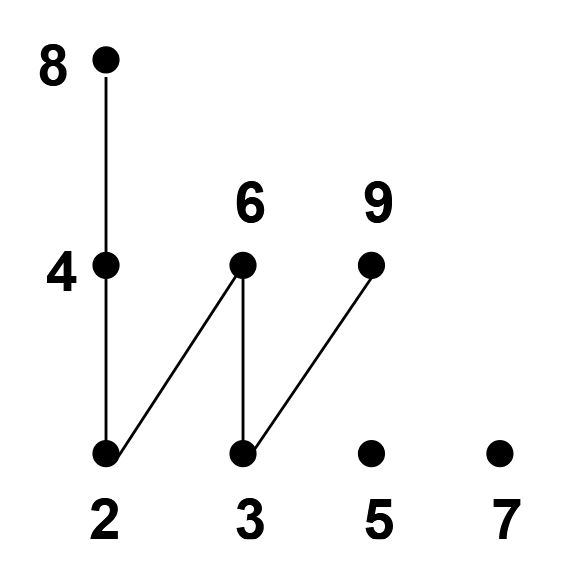
- Minimal elements: \(2, 3, 5, 7\) (primes)
- Maximal elements: \(5, 6, 7, 8, 9\)
- Least or greatest element: There is none (not all elements comparable)
Back
Consider the poset \((\{2, 3, 4, 5, 6, 7, 8, 9\}; |)\).
- Minimal elements: \(2, 3, 5, 7\) (primes)
- Maximal elements: \(5, 6, 7, 8, 9\)
- Least or greatest element: There is none (not all elements comparable)
Current
Note has been deleted
Field-by-field Comparison
| Field | Before | After |
|---|---|---|
| Text |
Note 868: ETH::1. Semester::DiskMat
Deck: ETH::1. Semester::DiskMat
Note Type: Horvath Classic
GUID:
deleted
Note Type: Horvath Classic
GUID:
pmg@X@cPde
Deleted Note
Front
How can we simplify \(R_m(f(a_1, \dots, a_k))\) for a polynomial \(f\)? (Corollary 4.17)
Back
How can we simplify \(R_m(f(a_1, \dots, a_k))\) for a polynomial \(f\)? (Corollary 4.17)
\[R_m(f(a_1, \dots, a_k)) = R_m(f(R_m(a_1), \dots, R_m(a_k)))\]
We can first reduce each argument modulo \(m\), then evaluate the polynomial.
Current
Note has been deleted
Field-by-field Comparison
| Field | Before | After |
|---|---|---|
| Front | ||
| Back |
Note 869: ETH::1. Semester::DiskMat
Deck: ETH::1. Semester::DiskMat
Note Type: Horvath Cloze
GUID:
deleted
Note Type: Horvath Cloze
GUID:
px2&&RIh%e
Deleted Note
Front
In any non-trivial ring \(\langle R; +, -, 0, \cdot, 1 \rangle\) \(1 \neq 0\) holds.
Back
In any non-trivial ring \(\langle R; +, -, 0, \cdot, 1 \rangle\) \(1 \neq 0\) holds.
If \(1=0\), then for all \(a \in R\) : \(a=1⋅a=0⋅a=0\)
So the ring would be trivial (only contains 0).
Current
Note has been deleted
Field-by-field Comparison
| Field | Before | After |
|---|---|---|
| Text | ||
| Extra |
Note 870: ETH::1. Semester::DiskMat
Deck: ETH::1. Semester::DiskMat
Note Type: Horvath Classic
GUID:
deleted
Note Type: Horvath Classic
GUID:
p|78(#x<7
Deleted Note
Front
When is a relation \(\rho\) on set \(A\) transitive?
Back
When is a relation \(\rho\) on set \(A\) transitive?
When \(a \ \rho \ b \land b \ \rho \ c \Rightarrow a \ \rho \ c\) for all \(a, b, c \in A\).
Current
Note has been deleted
Field-by-field Comparison
| Field | Before | After |
|---|---|---|
| Front | ||
| Back |
Note 871: ETH::1. Semester::DiskMat
Deck: ETH::1. Semester::DiskMat
Note Type: Horvath Classic
GUID:
deleted
Note Type: Horvath Classic
GUID:
p~hk22.~%D
Deleted Note
Front
What is the relationship between tautologies and unsatisfiable formulas?
Back
What is the relationship between tautologies and unsatisfiable formulas?
A formula \(F\) is a tautology if and only if \(\lnot F\) is unsatisfiable.
Current
Note has been deleted
Field-by-field Comparison
| Field | Before | After |
|---|---|---|
| Front | ||
| Back |
Note 872: ETH::1. Semester::DiskMat
Deck: ETH::1. Semester::DiskMat
Note Type: Horvath Cloze
GUID:
deleted
Note Type: Horvath Cloze
GUID:
q%i_)pDyvo
Deleted Note
Front
A prominent example for an uncomputable function is the Halting problem.
Back
A prominent example for an uncomputable function is the Halting problem.
Given as input a program (encoded as a bit-string or natural number) together with an input (to the program), determine whether the program will eventually stop (function value 1) or loop forever (function value 0) on that input.
This function is uncomputable. If a halting-decider existed, one could build a program that uses it to do the opposite of what the decider predicts about itself, creating a contradiction: it halts if the halting program returns 0, and does not halt if it returns 1.
This is usually stated as: The Halting problem is undecidable.
Current
Note has been deleted
Field-by-field Comparison
| Field | Before | After |
|---|---|---|
| Text | ||
| Extra |
Note 873: ETH::1. Semester::DiskMat
Deck: ETH::1. Semester::DiskMat
Note Type: Horvath Classic
GUID:
deleted
Note Type: Horvath Classic
GUID:
q+.5DlE?)<
Deleted Note
Front
Give the formal definition of Cartesian product \(A \times B\).
Back
Give the formal definition of Cartesian product \(A \times B\).
\[A \times B = \{(a, b) \ | \ a \in A \land b \in B\}\]
The set of all ordered pairs with first component from \(A\) and second from \(B\).
Current
Note has been deleted
Field-by-field Comparison
| Field | Before | After |
|---|---|---|
| Front | ||
| Back |
Note 874: ETH::1. Semester::DiskMat
Deck: ETH::1. Semester::DiskMat
Note Type: Horvath Classic
GUID:
deleted
Note Type: Horvath Classic
GUID:
q+Di!TuDdT
Deleted Note
Front
How many divisors does \(n\) expressed as a factor of prime numbers \(n = \prod_{i = 1}^m p_i^{e_i}\) have?
Back
How many divisors does \(n\) expressed as a factor of prime numbers \(n = \prod_{i = 1}^m p_i^{e_i}\) have?
\(n\) has \(\# _ {\text{div}(n)} = \prod_{i = 1}^m (e_i + 1)\) divisors.
Current
Note has been deleted
Field-by-field Comparison
| Field | Before | After |
|---|---|---|
| Front | ||
| Back |
Note 875: ETH::1. Semester::DiskMat
Deck: ETH::1. Semester::DiskMat
Note Type: Horvath Cloze
GUID:
deleted
Note Type: Horvath Cloze
GUID:
q={`z2{i#x
Deleted Note
Front
We can transform every formula into:
- Prenex
- CNF
- DNF
- Skolem
Back
We can transform every formula into:
- Prenex
- CNF
- DNF
- Skolem
Current
Note has been deleted
Field-by-field Comparison
| Field | Before | After |
|---|---|---|
| Text |
Note 876: ETH::1. Semester::DiskMat
Deck: ETH::1. Semester::DiskMat
Note Type: Horvath Classic
GUID:
deleted
Note Type: Horvath Classic
GUID:
q?95w$fJDO
Deleted Note
Front
What is \(F[x]_{m(x)}\)?
Back
What is \(F[x]_{m(x)}\)?
Let \(m(x)\) be a polynomial of degree \(d\) over \(F\). Then: \[F[x]_{m(x)} \ \overset{\text{def}}{=} \ \{a(x) \in F[x] \ | \ \deg(a(x)) < d\}\]
This is the set of all polynomials over \(F\) with degree strictly less than \(d\).
Current
Note has been deleted
Field-by-field Comparison
| Field | Before | After |
|---|---|---|
| Front | ||
| Back |
Note 877: ETH::1. Semester::DiskMat
Deck: ETH::1. Semester::DiskMat
Note Type: Horvath Classic
GUID:
deleted
Note Type: Horvath Classic
GUID:
qAyHDnFN7L
Deleted Note
Front
What is the number of generators of \(\mathbb{Z}_n^*\)?
Back
What is the number of generators of \(\mathbb{Z}_n^*\)?
1. Verify that \(\mathbb{Z}_n^*\)is cyclic (iff n = 2, 4, \(p^e\), \(2p^e\), with \(e \ge 1\) and \(p\) is an odd prime)
2. If \(\mathbb{Z}_n^*\) is cyclic then it is isomorphic to \(\mathbb{Z}_{\varphi(n)}^+\) (by Lemma)
3. The number of generators of \(\mathbb{Z}_{\varphi(n)}^+\) is \(\varphi(\varphi(n))\) as it is the number of elements coprime to the group order.
2. If \(\mathbb{Z}_n^*\) is cyclic then it is isomorphic to \(\mathbb{Z}_{\varphi(n)}^+\) (by Lemma)
3. The number of generators of \(\mathbb{Z}_{\varphi(n)}^+\) is \(\varphi(\varphi(n))\) as it is the number of elements coprime to the group order.
Current
Note has been deleted
Field-by-field Comparison
| Field | Before | After |
|---|---|---|
| Front | ||
| Back |
Note 878: ETH::1. Semester::DiskMat
Deck: ETH::1. Semester::DiskMat
Note Type: Horvath Cloze
GUID:
deleted
Note Type: Horvath Cloze
GUID:
qFQ3yDTc>-
Deleted Note
Front
An element \(u\) of a ring \(R\) is called a unit if \(u\) is invertible.
Back
An element \(u\) of a ring \(R\) is called a unit if \(u\) is invertible.
Current
Note has been deleted
Field-by-field Comparison
| Field | Before | After |
|---|---|---|
| Text |
Note 879: ETH::1. Semester::DiskMat
Deck: ETH::1. Semester::DiskMat
Note Type: Horvath Cloze
GUID:
deleted
Note Type: Horvath Cloze
GUID:
qFYoZgCSMu
Deleted Note
Front
The predicate \(\tau\) defines the set {{c1::of strings \(L \subseteq \{0, 1\}\) that correspond to true statements}}.
Back
The predicate \(\tau\) defines the set {{c1::of strings \(L \subseteq \{0, 1\}\) that correspond to true statements}}.
Current
Note has been deleted
Field-by-field Comparison
| Field | Before | After |
|---|---|---|
| Text |
Note 880: ETH::1. Semester::DiskMat
Deck: ETH::1. Semester::DiskMat
Note Type: Horvath Cloze
GUID:
deleted
Note Type: Horvath Cloze
GUID:
qScQPkEg%q
Deleted Note
Front
A logical formula is generally not a mathematical statement, because the truth value depends on the interpretation of the symbols.
Back
A logical formula is generally not a mathematical statement, because the truth value depends on the interpretation of the symbols.
(so we can't prove/disprove it)
Current
Note has been deleted
Field-by-field Comparison
| Field | Before | After |
|---|---|---|
| Text | ||
| Extra |
Note 881: ETH::1. Semester::DiskMat
Deck: ETH::1. Semester::DiskMat
Note Type: Horvath Classic
GUID:
deleted
Note Type: Horvath Classic
GUID:
q[i&,qVWc9
Deleted Note
Front
What is modular congruence in a polynomial field?
Back
What is modular congruence in a polynomial field?
\[a(x) \equiv_{m(x)} b(x) \quad \overset{\text{def}}{\Leftrightarrow} \quad m(x) \ | \ (a(x) - b(x))\]
Current
Note has been deleted
Field-by-field Comparison
| Field | Before | After |
|---|---|---|
| Front | ||
| Back |
Note 882: ETH::1. Semester::DiskMat
Deck: ETH::1. Semester::DiskMat
Note Type: Horvath Classic
GUID:
deleted
Note Type: Horvath Classic
GUID:
q]nbKvbP{^
Deleted Note
Front
In a field, you can:
Back
In a field, you can:
- add
- subtract
- multiply
- divide by any nonzero element.
You can divide, because in a field the multiplicative monoid is also a group (without \(0\), thus \(0\) cannot be divided by - no inverse).
Current
Note has been deleted
Field-by-field Comparison
| Field | Before | After |
|---|---|---|
| Front | ||
| Back |
Note 883: ETH::1. Semester::DiskMat
Deck: ETH::1. Semester::DiskMat
Note Type: Horvath Classic
GUID:
deleted
Note Type: Horvath Classic
GUID:
q_~/j+G,$p
Deleted Note
Front
What is the fundamental theorem of arithmetic?
Back
What is the fundamental theorem of arithmetic?
Every positive integer can be written uniquely as the product of primes.
Current
Note has been deleted
Field-by-field Comparison
| Field | Before | After |
|---|---|---|
| Front | ||
| Back |
Note 884: ETH::1. Semester::DiskMat
Deck: ETH::1. Semester::DiskMat
Note Type: Horvath Cloze
GUID:
deleted
Note Type: Horvath Cloze
GUID:
qi1M.
Deleted Note
Front
When an operation is associative, \(a_1 * a_2 * \dots * a_n\) is independent of the order of execution.
Back
When an operation is associative, \(a_1 * a_2 * \dots * a_n\) is independent of the order of execution.
Current
Note has been deleted
Field-by-field Comparison
| Field | Before | After |
|---|---|---|
| Text |
Note 885: ETH::1. Semester::DiskMat
Deck: ETH::1. Semester::DiskMat
Note Type: Horvath Cloze
GUID:
deleted
Note Type: Horvath Cloze
GUID:
qnpI?yoaky
Deleted Note
Front
What are the three properties of a partial order relation?
- Reflexivity
- Antisymmetry
- Transitivity
Back
What are the three properties of a partial order relation?
- Reflexivity
- Antisymmetry
- Transitivity
Current
Note has been deleted
Field-by-field Comparison
| Field | Before | After |
|---|---|---|
| Text |
Note 886: ETH::1. Semester::DiskMat
Deck: ETH::1. Semester::DiskMat
Note Type: Horvath Cloze
GUID:
deleted
Note Type: Horvath Cloze
GUID:
qo:})x5a6`
Deleted Note
Front
In a group, the equations \(a * x = b\) and \(x * a = b\) have unique solutions for all \(a, b\) (property G3(v)).
Back
In a group, the equations \(a * x = b\) and \(x * a = b\) have unique solutions for all \(a, b\) (property G3(v)).
Current
Note has been deleted
Field-by-field Comparison
| Field | Before | After |
|---|---|---|
| Text |
Note 887: ETH::1. Semester::DiskMat
Deck: ETH::1. Semester::DiskMat
Note Type: Horvath Classic
GUID:
deleted
Note Type: Horvath Classic
GUID:
qx(`A-^(T{
Deleted Note
Front
Definition of irreflexive
Back
Definition of irreflexive
A relation \(\rho\) on a set A is called irreflexive if \(a \ \not \rho \ a\) for all a ∈ A, i.e., if \(\rho \ \cap \ \text{id} = \emptyset\).
Not that this is not the negation of reflexive!
Not that this is not the negation of reflexive!
Current
Note has been deleted
Field-by-field Comparison
| Field | Before | After |
|---|---|---|
| Front | ||
| Back |
Note 888: ETH::1. Semester::DiskMat
Deck: ETH::1. Semester::DiskMat
Note Type: Horvath Cloze
GUID:
deleted
Note Type: Horvath Cloze
GUID:
q|}rXYFly~
Deleted Note
Front
Euler's totient function \(\varphi: \mathbb{Z}^+ \rightarrow \mathbb{Z}^+\) is defined as {{c2::the cardinality of \(\mathbb{Z}_m^*\): \[\varphi(m) = |\mathbb{Z}_m^*|\]}}
Back
Euler's totient function \(\varphi: \mathbb{Z}^+ \rightarrow \mathbb{Z}^+\) is defined as {{c2::the cardinality of \(\mathbb{Z}_m^*\): \[\varphi(m) = |\mathbb{Z}_m^*|\]}}
Current
Note has been deleted
Field-by-field Comparison
| Field | Before | After |
|---|---|---|
| Text |
Note 889: ETH::1. Semester::DiskMat
Deck: ETH::1. Semester::DiskMat
Note Type: Horvath Classic
GUID:
deleted
Note Type: Horvath Classic
GUID:
r.P@LlU$vR
Deleted Note
Front
Give the formal definition of the least common multiple \(\text{lcm}(a, b)\).
Back
Give the formal definition of the least common multiple \(\text{lcm}(a, b)\).
\[a \mid l \land b \mid l \land \forall m \ ((a \mid m \land b \mid m) \rightarrow l \mid m)\]
\(l\) is a common multiple of \(a\) and \(b\) which divides every common multiple of \(a\) and \(b\).
Current
Note has been deleted
Field-by-field Comparison
| Field | Before | After |
|---|---|---|
| Front | ||
| Back |
Note 890: ETH::1. Semester::DiskMat
Deck: ETH::1. Semester::DiskMat
Note Type: Horvath Classic
GUID:
deleted
Note Type: Horvath Classic
GUID:
r3)589~fN6
Deleted Note
Front
What is the cardinality of \(F[x]_{m(x)}\)?
Back
What is the cardinality of \(F[x]_{m(x)}\)?
Lemma 5.34: Let \(F\) be a finite field with \(q\) elements and let \(m(x)\) be a polynomial of degree \(d\) over \(F\). Then: \[|F[x]_{m(x)}| = q^d\]
Explanation: Each polynomial of \(\deg d - 1\) has \(d\) coefficients (from \(0, \dots, d - 1\)), and each coefficient can be any of \(q\) elements from \(F\).
Current
Note has been deleted
Field-by-field Comparison
| Field | Before | After |
|---|---|---|
| Front | ||
| Back |
Note 891: ETH::1. Semester::DiskMat
Deck: ETH::1. Semester::DiskMat
Note Type: Horvath Classic
GUID:
deleted
Note Type: Horvath Classic
GUID:
rI[60?4iFu
Deleted Note
Front
A group has the following properties:
Back
A group has the following properties:
- Closure
- Associativity
- Identity
- Inverse
Current
Note has been deleted
Field-by-field Comparison
| Field | Before | After |
|---|---|---|
| Front | ||
| Back |
Note 892: ETH::1. Semester::DiskMat
Deck: ETH::1. Semester::DiskMat
Note Type: Horvath Cloze
GUID:
deleted
Note Type: Horvath Cloze
GUID:
rMrK0z!nVO
Deleted Note
Front
In a cyclic group \(\langle g \rangle\), associativity is inherited from the parent group \(G\).
Back
In a cyclic group \(\langle g \rangle\), associativity is inherited from the parent group \(G\).
Current
Note has been deleted
Field-by-field Comparison
| Field | Before | After |
|---|---|---|
| Text |
Note 893: ETH::1. Semester::DiskMat
Deck: ETH::1. Semester::DiskMat
Note Type: Horvath Cloze
GUID:
deleted
Note Type: Horvath Cloze
GUID:
rU5OFOfB=/
Deleted Note
Front
In any commutative ring, if \(a \ | \ b\) then \(a \ | \ bc\) for all \(c\).
Back
In any commutative ring, if \(a \ | \ b\) then \(a \ | \ bc\) for all \(c\).
Current
Note has been deleted
Field-by-field Comparison
| Field | Before | After |
|---|---|---|
| Text |
Note 894: ETH::1. Semester::DiskMat
Deck: ETH::1. Semester::DiskMat
Note Type: Horvath Cloze
GUID:
deleted
Note Type: Horvath Cloze
GUID:
rkyD`Rw*Nl
Deleted Note
Front
We are allowed to swap quantifier order in a formula if:
- they are of the same type
- the variables never appear in the same predicate
Back
We are allowed to swap quantifier order in a formula if:
- they are of the same type
- the variables never appear in the same predicate
Current
Note has been deleted
Field-by-field Comparison
| Field | Before | After |
|---|---|---|
| Text |
Note 895: ETH::1. Semester::DiskMat
Deck: ETH::1. Semester::DiskMat
Note Type: Horvath Classic
GUID:
deleted
Note Type: Horvath Classic
GUID:
rz^&c?ddI>
Deleted Note
Front
G is a logical conseqence of F. What does that mean?
Back
G is a logical conseqence of F. What does that mean?
\( F \models G\) if G is always true if F is true, but not necessarily false when F is false. (No causality!)
Current
Note has been deleted
Field-by-field Comparison
| Field | Before | After |
|---|---|---|
| Front | ||
| Back |
Note 896: ETH::1. Semester::DiskMat
Deck: ETH::1. Semester::DiskMat
Note Type: Horvath Cloze
GUID:
deleted
Note Type: Horvath Cloze
GUID:
s$,Xim%,O5
Deleted Note
Front
Lemma 5.22(3): The units of \(D[x]\) are the constant polynomials that are units of \(D\): \(D[x]^* = D^*\).
Back
Lemma 5.22(3): The units of \(D[x]\) are the constant polynomials that are units of \(D\): \(D[x]^* = D^*\).
Current
Note has been deleted
Field-by-field Comparison
| Field | Before | After |
|---|---|---|
| Text |
Note 897: ETH::1. Semester::DiskMat
Deck: ETH::1. Semester::DiskMat
Note Type: Horvath Cloze
GUID:
deleted
Note Type: Horvath Cloze
GUID:
s&thqL60qD
Deleted Note
Front
For \(a,b,m\in\mathbb{Z}\) with \(m\ge1\), we say that \(a\) is congruent to \(b\) modulo \(m\) if \(m\) divides \(a-b\).
Written as an expression: \(a\equiv_mb \iff m \mid (a-b)\).
Written as an expression: \(a\equiv_mb \iff m \mid (a-b)\).
Back
For \(a,b,m\in\mathbb{Z}\) with \(m\ge1\), we say that \(a\) is congruent to \(b\) modulo \(m\) if \(m\) divides \(a-b\).
Written as an expression: \(a\equiv_mb \iff m \mid (a-b)\).
Written as an expression: \(a\equiv_mb \iff m \mid (a-b)\).
Current
Note has been deleted
Field-by-field Comparison
| Field | Before | After |
|---|---|---|
| Text |
Note 898: ETH::1. Semester::DiskMat
Deck: ETH::1. Semester::DiskMat
Note Type: Horvath Cloze
GUID:
deleted
Note Type: Horvath Cloze
GUID:
s(DE`)q*(T
Deleted Note
Front
A partial order on a set \(A\) is a relation that is:
- reflexive
- antisymmetric
- transitive
Back
A partial order on a set \(A\) is a relation that is:
- reflexive
- antisymmetric
- transitive
Examples: \(\leq, \geq\)
Current
Note has been deleted
Field-by-field Comparison
| Field | Before | After |
|---|---|---|
| Text | ||
| Extra |
Note 899: ETH::1. Semester::DiskMat
Deck: ETH::1. Semester::DiskMat
Note Type: Horvath Cloze
GUID:
deleted
Note Type: Horvath Cloze
GUID:
s*8T*K?3f=
Deleted Note
Front
A function \(f: A \rightarrow B\) has a left inverse if and only if \(f\) is injective (not in script).
Back
A function \(f: A \rightarrow B\) has a left inverse if and only if \(f\) is injective (not in script).
Current
Note has been deleted
Field-by-field Comparison
| Field | Before | After |
|---|---|---|
| Text |
Note 900: ETH::1. Semester::DiskMat
Deck: ETH::1. Semester::DiskMat
Note Type: Horvath Cloze
GUID:
deleted
Note Type: Horvath Cloze
GUID:
s2,pAWT0;U
Deleted Note
Front
An irreducible polynomial of degree \(\geq 2\) has no roots.
Back
An irreducible polynomial of degree \(\geq 2\) has no roots.
Current
Note has been deleted
Field-by-field Comparison
| Field | Before | After |
|---|---|---|
| Text |
Note 901: ETH::1. Semester::DiskMat
Deck: ETH::1. Semester::DiskMat
Note Type: Horvath Cloze
GUID:
deleted
Note Type: Horvath Cloze
GUID:
s4qU[:Rl0m
Deleted Note
Front
A poset \((A; \preceq)\) is called totally ordered (also: linearly ordered) by \(\preceq\) if any two elements of the poset are comparable.
Back
A poset \((A; \preceq)\) is called totally ordered (also: linearly ordered) by \(\preceq\) if any two elements of the poset are comparable.
Example: \((\mathbb{Z}; \ge)\)
Current
Note has been deleted
Field-by-field Comparison
| Field | Before | After |
|---|---|---|
| Text | ||
| Extra |
Note 902: ETH::1. Semester::DiskMat
Deck: ETH::1. Semester::DiskMat
Note Type: Horvath Classic
GUID:
deleted
Note Type: Horvath Classic
GUID:
s7*HAj`,kR
Deleted Note
Front
Name four examples for (binary) relations as defined in discrete mathematics.
Back
Name four examples for (binary) relations as defined in discrete mathematics.
\(=, \ne, \le, \ge, <, >, \mid, \dots\)
Current
Note has been deleted
Field-by-field Comparison
| Field | Before | After |
|---|---|---|
| Front | ||
| Back |
Note 903: ETH::1. Semester::DiskMat
Deck: ETH::1. Semester::DiskMat
Note Type: Horvath Classic
GUID:
deleted
Note Type: Horvath Classic
GUID:
s>%Mz^.26_
Deleted Note
Front
Name a zerodivisor in a ring.
Back
Name a zerodivisor in a ring.
\(2\) is a zerodivisor of \(\mathbb{Z}_4\), as \(2*2 = 0\).
Current
Note has been deleted
Field-by-field Comparison
| Field | Before | After |
|---|---|---|
| Front | ||
| Back |
Note 904: ETH::1. Semester::DiskMat
Deck: ETH::1. Semester::DiskMat
Note Type: Horvath Classic
GUID:
deleted
Note Type: Horvath Classic
GUID:
s?tB!9azRK
Deleted Note
Front
An abelian group has the following properties:
Back
An abelian group has the following properties:
- closure
- associativity
- identity
- inverse
- commutative
Current
Note has been deleted
Field-by-field Comparison
| Field | Before | After |
|---|---|---|
| Front | ||
| Back |
Note 905: ETH::1. Semester::DiskMat
Deck: ETH::1. Semester::DiskMat
Note Type: Horvath Cloze
GUID:
deleted
Note Type: Horvath Cloze
GUID:
sQoa!PVGy1
Deleted Note
Front
\(\mathbb{Z}_m^*\) is more useful than \(\mathbb{Z}_m\), because {{c1::\(\mathbb{Z}_m\)is not a group with respect to multiplication modulo \(m\), which we would need for RSA}}.
Back
\(\mathbb{Z}_m^*\) is more useful than \(\mathbb{Z}_m\), because {{c1::\(\mathbb{Z}_m\)is not a group with respect to multiplication modulo \(m\), which we would need for RSA}}.
Not all elements in \(\mathbb{Z}_m\) have an inverse, something which \(\mathbb{Z}_m^*\) on the other hand guarantees via Bézout.
Current
Note has been deleted
Field-by-field Comparison
| Field | Before | After |
|---|---|---|
| Text | ||
| Extra |
Note 906: ETH::1. Semester::DiskMat
Deck: ETH::1. Semester::DiskMat
Note Type: Horvath Classic
GUID:
deleted
Note Type: Horvath Classic
GUID:
sXwCtB@o/s
Deleted Note
Front
What \(a \in \mathbb{Z}_n\) generate \(\mathbb{Z}_n\)?
Back
What \(a \in \mathbb{Z}_n\) generate \(\mathbb{Z}_n\)?
All \(a \in \mathbb{Z}_n\) such that \(\gcd(a, n) = 1\).
-
If \(\gcd(a,n) = d > 1\), then all multiples of a are divisible by d, so you only hit every d-th residue mod n.
-
If \(\gcd(a,n) = 1\), then multiples of a eventually hit every residue class mod n.
Current
Note has been deleted
Field-by-field Comparison
| Field | Before | After |
|---|---|---|
| Front | ||
| Back |
Note 907: ETH::1. Semester::DiskMat
Deck: ETH::1. Semester::DiskMat
Note Type: Horvath Cloze
GUID:
deleted
Note Type: Horvath Cloze
GUID:
s[Y-0E4#sz
Deleted Note
Front
A ring \(\langle R, +, -, 0, \cdot, 1 \rangle\) is an algebra with the properties that
- \(\langle R, +, -, 0 \rangle\) is a commutative group
- \(\langle R, \cdot, 1 \rangle\) is a monoid
- \( a(b+c) = (ab) + (ac), (b+c)a = (ba) + (ca)\) (left and right distributive laws)
Back
A ring \(\langle R, +, -, 0, \cdot, 1 \rangle\) is an algebra with the properties that
- \(\langle R, +, -, 0 \rangle\) is a commutative group
- \(\langle R, \cdot, 1 \rangle\) is a monoid
- \( a(b+c) = (ab) + (ac), (b+c)a = (ba) + (ca)\) (left and right distributive laws)
Examples: \(\mathbb{Z}, \mathbb{R}\)
Current
Note has been deleted
Field-by-field Comparison
| Field | Before | After |
|---|---|---|
| Text | ||
| Extra |
Note 908: ETH::1. Semester::DiskMat
Deck: ETH::1. Semester::DiskMat
Note Type: Horvath Cloze
GUID:
deleted
Note Type: Horvath Cloze
GUID:
s[dJ]w
Deleted Note
Front
A relation \(ρ\) on a set \(A\) is called antisymmetric if {{c1::\( a \ \rho \ b \wedge b \ \rho \ a \implies a = b\) is true, i.e. if \( \rho \cap \hat{\rho} \subseteq \text{id}\)}}
Back
A relation \(ρ\) on a set \(A\) is called antisymmetric if {{c1::\( a \ \rho \ b \wedge b \ \rho \ a \implies a = b\) is true, i.e. if \( \rho \cap \hat{\rho} \subseteq \text{id}\)}}
Example: \( \le, \ge\) and the division relation: \( a \mid b \wedge b \mid a \implies a = b\)
Current
Note has been deleted
Field-by-field Comparison
| Field | Before | After |
|---|---|---|
| Text | ||
| Extra |
Note 909: ETH::1. Semester::DiskMat
Deck: ETH::1. Semester::DiskMat
Note Type: Horvath Classic
GUID:
deleted
Note Type: Horvath Classic
GUID:
s]+I0[)5QL
Deleted Note
Front
Show that \(\mathbb{Z}\) is countable by exhibiting a bijection with \(\mathbb{N}\).
Back
Show that \(\mathbb{Z}\) is countable by exhibiting a bijection with \(\mathbb{N}\).
The function \(f(n) = (-1)^n \lceil n/2 \rceil\) is a bijection \(\mathbb{N} \to \mathbb{Z}\).
Maps: \(0 \mapsto 0, 1 \mapsto 1, 2 \mapsto -1, 3 \mapsto 2, 4 \mapsto -2, \ldots\)
Maps: \(0 \mapsto 0, 1 \mapsto 1, 2 \mapsto -1, 3 \mapsto 2, 4 \mapsto -2, \ldots\)
Current
Note has been deleted
Field-by-field Comparison
| Field | Before | After |
|---|---|---|
| Front | ||
| Back |
Note 910: ETH::1. Semester::DiskMat
Deck: ETH::1. Semester::DiskMat
Note Type: Horvath Cloze
GUID:
deleted
Note Type: Horvath Cloze
GUID:
s`dg
Deleted Note
Front
If both \(b * a = e\) and \(a * b = e\), then \(b\) is simply called an inverse of \(a\).
Back
If both \(b * a = e\) and \(a * b = e\), then \(b\) is simply called an inverse of \(a\).
Current
Note has been deleted
Field-by-field Comparison
| Field | Before | After |
|---|---|---|
| Text |
Note 911: ETH::1. Semester::DiskMat
Deck: ETH::1. Semester::DiskMat
Note Type: Horvath Classic
GUID:
deleted
Note Type: Horvath Classic
GUID:
sjn:t.?:uH
Deleted Note
Front
What are the two steps of a proof by induction?
Back
What are the two steps of a proof by induction?
1. Basis Step: Prove \(P(0)\) (or \(P(1)\) or \(P(k)\) depending on universe)
2. Induction Step: Prove that for any arbitrary \(n\), \(P(n) \Rightarrow P(n+1)\) (assuming \(P(n)\) as the induction hypothesis)
2. Induction Step: Prove that for any arbitrary \(n\), \(P(n) \Rightarrow P(n+1)\) (assuming \(P(n)\) as the induction hypothesis)
Current
Note has been deleted
Field-by-field Comparison
| Field | Before | After |
|---|---|---|
| Front | ||
| Back |
Note 912: ETH::1. Semester::DiskMat
Deck: ETH::1. Semester::DiskMat
Note Type: Horvath Classic
GUID:
deleted
Note Type: Horvath Classic
GUID:
sxW-Trt$`+
Deleted Note
Front
\(\mathbb{Z}_m^*\) is defined as?
Back
\(\mathbb{Z}_m^*\) is defined as?
\[ \overset{\text{def}}{=} \ \{a \in \mathbb{Z}_m \ | \ \gcd(a, m) = 1\} \]
This is the set of all elements in \(\mathbb{Z}_m\) that are coprime to \(m\).
Current
Note has been deleted
Field-by-field Comparison
| Field | Before | After |
|---|---|---|
| Front | ||
| Back |
Note 913: ETH::1. Semester::DiskMat
Deck: ETH::1. Semester::DiskMat
Note Type: Horvath Cloze
GUID:
deleted
Note Type: Horvath Cloze
GUID:
t$?o*APa?u
Deleted Note
Front
We denote the field with \(p\) elements (where \(p\) is prime) by {{c2::\(\text{GF}(p)\) rather than \(\mathbb{Z}_p\)}}.
Back
We denote the field with \(p\) elements (where \(p\) is prime) by {{c2::\(\text{GF}(p)\) rather than \(\mathbb{Z}_p\)}}.
Current
Note has been deleted
Field-by-field Comparison
| Field | Before | After |
|---|---|---|
| Text |
Note 914: ETH::1. Semester::DiskMat
Deck: ETH::1. Semester::DiskMat
Note Type: Horvath Classic
GUID:
deleted
Note Type: Horvath Classic
GUID:
t4rUQSlGPE
Deleted Note
Front
For what types of posets is well-ordering primarily of interest?
Back
For what types of posets is well-ordering primarily of interest?
Infinite posets.
(Every totally ordered finite poset is automatically well-ordered)
(Every totally ordered finite poset is automatically well-ordered)
Current
Note has been deleted
Field-by-field Comparison
| Field | Before | After |
|---|---|---|
| Front | ||
| Back |
Note 915: ETH::1. Semester::DiskMat
Deck: ETH::1. Semester::DiskMat
Note Type: Horvath Classic
GUID:
deleted
Note Type: Horvath Classic
GUID:
tBd|.5x#E:
Deleted Note
Front
How is the lexicographic order \(\leq_{\text{lex}}\) on \(A \times B\) defined?
Back
How is the lexicographic order \(\leq_{\text{lex}}\) on \(A \times B\) defined?
\[(a_1, b_1) \leq_{\text{lex}} (a_2, b_2) \overset{\text{def}}{\Longleftrightarrow} a_1 \prec a_2 \lor (a_1 = a_2 \land b_1 \sqsubseteq b_2)\]
Current
Note has been deleted
Field-by-field Comparison
| Field | Before | After |
|---|---|---|
| Front | ||
| Back |
Note 916: ETH::1. Semester::DiskMat
Deck: ETH::1. Semester::DiskMat
Note Type: Horvath Cloze
GUID:
deleted
Note Type: Horvath Cloze
GUID:
tNw~Zi`Up.
Deleted Note
Front
In any commutative ring: If \(a \ | \ b\) and \(b \ | \ c\) then \(a \ | \ c\), i.e. the relation | is transitive.
Back
In any commutative ring: If \(a \ | \ b\) and \(b \ | \ c\) then \(a \ | \ c\), i.e. the relation | is transitive.
Current
Note has been deleted
Field-by-field Comparison
| Field | Before | After |
|---|---|---|
| Text |
Note 917: ETH::1. Semester::DiskMat
Deck: ETH::1. Semester::DiskMat
Note Type: Horvath Classic
GUID:
deleted
Note Type: Horvath Classic
GUID:
tXnVRUZ1r.
Deleted Note
Front
To show that a newly defined operator can be used to express any formula, we show that:
Back
To show that a newly defined operator can be used to express any formula, we show that:
\(\lnot F\), \(F \lor G\) and \(F \land G\) can be rewritten only in terms of it.
For example NOT, AND, OR can be expressed in NAND form, thus we can rewritten in CNF (or DNF) then NANDs (by simply replacing). As we can write every formula in CNF (or DNF) this prooves it.
For example NOT, AND, OR can be expressed in NAND form, thus we can rewritten in CNF (or DNF) then NANDs (by simply replacing). As we can write every formula in CNF (or DNF) this prooves it.
Current
Note has been deleted
Field-by-field Comparison
| Field | Before | After |
|---|---|---|
| Front | ||
| Back |
Note 918: ETH::1. Semester::DiskMat
Deck: ETH::1. Semester::DiskMat
Note Type: Horvath Classic
GUID:
deleted
Note Type: Horvath Classic
GUID:
tg<_s~pb{P
Deleted Note
Front
Proof method: "Composition of Implications"
Back
Proof method: "Composition of Implications"
Idea: If \( S \implies T \) and \( T \implies U \) are both true, then \( S \implies U \) is also true.
Current
Note has been deleted
Field-by-field Comparison
| Field | Before | After |
|---|---|---|
| Front | ||
| Back |
Note 919: ETH::1. Semester::DiskMat
Deck: ETH::1. Semester::DiskMat
Note Type: Horvath Classic
GUID:
deleted
Note Type: Horvath Classic
GUID:
tm%60;MTzw
Deleted Note
Front
What is a proof by counterexample?
Back
What is a proof by counterexample?
A proof that \(S_x\) is not true for all \(x \in X\) by exhibiting an \(a\) (called a counterexample) such that \(S_a\) is false.
Current
Note has been deleted
Field-by-field Comparison
| Field | Before | After |
|---|---|---|
| Front | ||
| Back |
Note 920: ETH::1. Semester::DiskMat
Deck: ETH::1. Semester::DiskMat
Note Type: Horvath Cloze
GUID:
deleted
Note Type: Horvath Cloze
GUID:
tm=T&mwo5w
Deleted Note
Front
The group denoted by \(\mathbb{Z}_n\) is always meant in conjunction with the operation \(\oplus\) modulo \(n\).
Back
The group denoted by \(\mathbb{Z}_n\) is always meant in conjunction with the operation \(\oplus\) modulo \(n\).
Current
Note has been deleted
Field-by-field Comparison
| Field | Before | After |
|---|---|---|
| Text |
Note 921: ETH::1. Semester::DiskMat
Deck: ETH::1. Semester::DiskMat
Note Type: Horvath Classic
GUID:
deleted
Note Type: Horvath Classic
GUID:
tmXe!J(6@%
Deleted Note
Front
Is antisymmetric the negation of symmetric?
Back
Is antisymmetric the negation of symmetric?
NO! Antisymmetry is NOT the negation of symmetry. They are independent properties.
A relation is both symmetric and antisymmetric if and only if it's a subset of the identity relation (i.e., \(R \subseteq \{(a, a) : a \in A\}\)). This includes the empty relation \(R = \emptyset\) as a degenerate case.
A relation is both symmetric and antisymmetric if and only if it's a subset of the identity relation (i.e., \(R \subseteq \{(a, a) : a \in A\}\)). This includes the empty relation \(R = \emptyset\) as a degenerate case.
Current
Note has been deleted
Field-by-field Comparison
| Field | Before | After |
|---|---|---|
| Front | ||
| Back |
Note 922: ETH::1. Semester::DiskMat
Deck: ETH::1. Semester::DiskMat
Note Type: Horvath Cloze
GUID:
deleted
Note Type: Horvath Cloze
GUID:
tpZRO@D#F:
Deleted Note
Front
Every polynomial of degree 4 is either irreducible or it has a factor of degree 1 or irreducible factor of degree 2.
Back
Every polynomial of degree 4 is either irreducible or it has a factor of degree 1 or irreducible factor of degree 2.
Current
Note has been deleted
Field-by-field Comparison
| Field | Before | After |
|---|---|---|
| Text |
Note 923: ETH::1. Semester::DiskMat
Deck: ETH::1. Semester::DiskMat
Note Type: Horvath Classic
GUID:
deleted
Note Type: Horvath Classic
GUID:
tuHe#n^N^#
Deleted Note
Front
The Diffie-Hellman Key-Agreement works because?
Back
The Diffie-Hellman Key-Agreement works because?
The discrete logarithm problem is hard!
That is, it's hard to find \(x_A\) from \(g^{x_A} \mod p\), knowing \(g\).
That is, it's hard to find \(x_A\) from \(g^{x_A} \mod p\), knowing \(g\).
Current
Note has been deleted
Field-by-field Comparison
| Field | Before | After |
|---|---|---|
| Front | ||
| Back |
Note 924: ETH::1. Semester::DiskMat
Deck: ETH::1. Semester::DiskMat
Note Type: Horvath Cloze
GUID:
deleted
Note Type: Horvath Cloze
GUID:
tz7t=t1v7n
Deleted Note
Front
\(F[x]\) is an integral domain.
Back
\(F[x]\) is an integral domain.
Current
Note has been deleted
Field-by-field Comparison
| Field | Before | After |
|---|---|---|
| Text |
Note 925: ETH::1. Semester::DiskMat
Deck: ETH::1. Semester::DiskMat
Note Type: Horvath Classic
GUID:
deleted
Note Type: Horvath Classic
GUID:
u${[$*iYrd
Deleted Note
Front
Does the uniqueness of the neutral element imply that a group is abelian (commutative)?
I.e. does \(a*e = e*a\) mean \(G\) is abelian?Back
Does the uniqueness of the neutral element imply that a group is abelian (commutative)?
I.e. does \(a*e = e*a\) mean \(G\) is abelian?No! The uniqueness of the neutral element does not imply commutativity.
Counterexample: The identity matrix \(I_3\) is the unique neutral element for the group of \(3 \times 3\) invertible real matrices under multiplication. We have \(A \cdot I_3 = I_3 \cdot A\) for all matrices \(A\), even though matrix multiplication is not commutative in general.
Current
Note has been deleted
Field-by-field Comparison
| Field | Before | After |
|---|---|---|
| Front | ||
| Back |
Note 926: ETH::1. Semester::DiskMat
Deck: ETH::1. Semester::DiskMat
Note Type: Horvath Classic
GUID:
deleted
Note Type: Horvath Classic
GUID:
u%LA!tL]Sb
Deleted Note
Front
What is a polynomial based encoding function?
Back
What is a polynomial based encoding function?
Theorem 5.42: Let \(\mathcal{A} = \text{GF}(q)\) and let \(\alpha_0, \dots, \alpha_{n-1}\) be arbitrary distinct elements of \(\text{GF}(q)\). Encode by polynomial evaluation: \[E((a_0, \dots, a_{k-1})) = (a(\alpha_0), \dots, a(\alpha_{n-1}))\] where \(a(x)\) is the polynomial with coefficients \((a_0, \dots, a_{k-1})\).
The code has minimum distance \(d_{\min} = n - k + 1\).
Key property: The polynomial can be interpolated from any \(k\) values by Lagrangian interpolation (b/c \(k\) coefficients = degree \(k-1\) due to the constant part of the polynomial). Two codewords cannot agree at \(k\) positions (else they'd be equal), i.e. they agree at most at \(k-1\) positions, so they disagree in at least \(n - k + 1\) positions.
Current
Note has been deleted
Field-by-field Comparison
| Field | Before | After |
|---|---|---|
| Front | ||
| Back |
Note 927: ETH::1. Semester::DiskMat
Deck: ETH::1. Semester::DiskMat
Note Type: Horvath Classic
GUID:
deleted
Note Type: Horvath Classic
GUID:
u*{HjaX,5R
Deleted Note
Front
In the lattice \((\{1,2,3,4,5,6,8,12,24\}; |)\), what are the meet and join for 6 and 8?
Back
In the lattice \((\{1,2,3,4,5,6,8,12,24\}; |)\), what are the meet and join for 6 and 8?
Meet: \(6 \land 8 = 2\) (gcd)
Join: \(6 \lor 8 = 24\) (lcm)
Current
Note has been deleted
Field-by-field Comparison
| Field | Before | After |
|---|---|---|
| Front | ||
| Back |
Note 928: ETH::1. Semester::DiskMat
Deck: ETH::1. Semester::DiskMat
Note Type: Horvath Classic
GUID:
deleted
Note Type: Horvath Classic
GUID:
u1$>B^csAD
Deleted Note
Front
How do you perform polynomial division when the divisor is not monic (e.g., in \(\text{GF}(7)[x]\))?
Back
How do you perform polynomial division when the divisor is not monic (e.g., in \(\text{GF}(7)[x]\))?
If dividing by a non-monic polynomial like \(4x + 2\) in \(\text{GF}(7)[x]\):
- Find the multiplicative inverse of the leading coefficient in the field
- For \(4\) in \(\text{GF}(7)\): \(4 \cdot 2 \equiv_7 1\), so \(4^{-1} = 2\)
- Multiply the polynomial by this inverse to make it monic
- \(2 \cdot (4x + 2) = 8x + 4 \equiv_7 x + 4\)
- Now divide by the monic polynomial
Example: \(3x^2 + 6x + 5\) divided by \(4x + 2\) becomes \(3x^2 + 6x + 5\) divided by \(\text{GF}(7)[x]\)0 (after multiplying by \(\text{GF}(7)[x]\)1).
Current
Note has been deleted
Field-by-field Comparison
| Field | Before | After |
|---|---|---|
| Front | ||
| Back |
Note 929: ETH::1. Semester::DiskMat
Deck: ETH::1. Semester::DiskMat
Note Type: Horvath Cloze
GUID:
deleted
Note Type: Horvath Cloze
GUID:
u3RL+}XGYF
Deleted Note
Front
The {{c2::power set of a set \(A\), denoted \(\mathcal{P}(A)\)}}, is the set of all subsets of \(A\).
Back
The {{c2::power set of a set \(A\), denoted \(\mathcal{P}(A)\)}}, is the set of all subsets of \(A\).
Current
Note has been deleted
Field-by-field Comparison
| Field | Before | After |
|---|---|---|
| Text |
Note 930: ETH::1. Semester::DiskMat
Deck: ETH::1. Semester::DiskMat
Note Type: Horvath Classic
GUID:
deleted
Note Type: Horvath Classic
GUID:
u7I279IY#p
Deleted Note
Front
When is there a finite field with \(q\) elements?
Back
When is there a finite field with \(q\) elements?
\(\text{GF}(q)\) is only finite if and only if \(q\) is a power of a prime, i.e. \(q = p^k\) for \(p\) prime.
Any two fields of the same size \(q\) are isomorphic.
Why: to construct an extension field, use \(\mathbb{Z}_p\) for coefficients. To be a field, \(p\) must be prime. In a polynomial with degree \(k-1\), each coefficient can take any of the \(p\) values from the coefficient field.
Current
Note has been deleted
Field-by-field Comparison
| Field | Before | After |
|---|---|---|
| Front | ||
| Back |
Note 931: ETH::1. Semester::DiskMat
Deck: ETH::1. Semester::DiskMat
Note Type: Horvath Cloze
GUID:
deleted
Note Type: Horvath Cloze
GUID:
u8U)|c~>_!
Deleted Note
Front
The degree of the sum of two polynomials is at most the maximum (can be smaller if the biggest coefficients cancel) of their degrees.
Back
The degree of the sum of two polynomials is at most the maximum (can be smaller if the biggest coefficients cancel) of their degrees.
Current
Note has been deleted
Field-by-field Comparison
| Field | Before | After |
|---|---|---|
| Text |
Note 932: ETH::1. Semester::DiskMat
Deck: ETH::1. Semester::DiskMat
Note Type: Horvath Classic
GUID:
deleted
Note Type: Horvath Classic
GUID:
uBR/x3yn=f
Deleted Note
Front
What is the principle of mathematical induction?
Back
What is the principle of mathematical induction?
For the universe \(\mathbb{N}\) and an arbitrary unary predicate \(P\):
\[P(0) \land \forall n (P(n) \rightarrow P(n+1)) \Rightarrow \forall n P(n)\]
(If the base case holds and the induction step holds, then the property holds for all natural numbers)
(If the base case holds and the induction step holds, then the property holds for all natural numbers)
Current
Note has been deleted
Field-by-field Comparison
| Field | Before | After |
|---|---|---|
| Front | ||
| Back |
Note 933: ETH::1. Semester::DiskMat
Deck: ETH::1. Semester::DiskMat
Note Type: Horvath Classic
GUID:
deleted
Note Type: Horvath Classic
GUID:
uCGhOduc{_
Deleted Note
Front
Explain the mechanical analog of the Diffie-Hellman protocol.
Back
Explain the mechanical analog of the Diffie-Hellman protocol.
A padlock without a key.
Alice and Bob can exchange their locks (closed) and keep a copy in the open state. Then they can both generate the same configuration, namely the two locks interlocked. For the adversary, this is impossible without breaking open one of the locks.
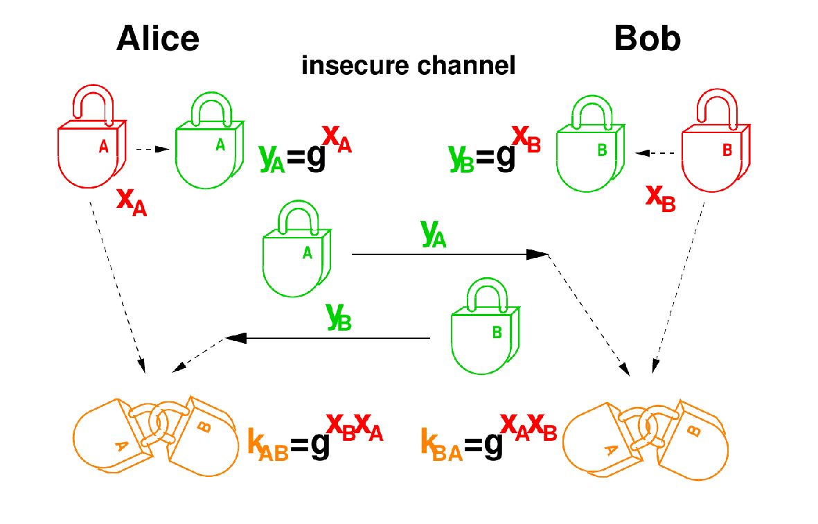
Alice and Bob can exchange their locks (closed) and keep a copy in the open state. Then they can both generate the same configuration, namely the two locks interlocked. For the adversary, this is impossible without breaking open one of the locks.
Current
Note has been deleted
Field-by-field Comparison
| Field | Before | After |
|---|---|---|
| Front | ||
| Back |
Note 934: ETH::1. Semester::DiskMat
Deck: ETH::1. Semester::DiskMat
Note Type: Horvath Classic
GUID:
deleted
Note Type: Horvath Classic
GUID:
uFE6t!4Hr%
Deleted Note
Front
A field has the following properties:
Back
A field has the following properties:
Additive Group:
- closure
- associativity
- identity
- inverse
- commutative
Multiplicative group:
- closure
- associativity
- distributivity
- identity
- no zero-divisor
- inverse
Current
Note has been deleted
Field-by-field Comparison
| Field | Before | After |
|---|---|---|
| Front | ||
| Back |
Note 935: ETH::1. Semester::DiskMat
Deck: ETH::1. Semester::DiskMat
Note Type: Horvath Classic
GUID:
deleted
Note Type: Horvath Classic
GUID:
uFN2l+&cfr
Deleted Note
Front
Can there be more than one neutral element?
Back
Can there be more than one neutral element?
No, \(\langle S; * \rangle\) can have at most one neutral element.
There can be a distinct left and right neutral though.
Example: \(3 \times 4\) matrices
There can be a distinct left and right neutral though.
Example: \(3 \times 4\) matrices
Current
Note has been deleted
Field-by-field Comparison
| Field | Before | After |
|---|---|---|
| Front | ||
| Back |
Note 936: ETH::1. Semester::DiskMat
Deck: ETH::1. Semester::DiskMat
Note Type: Horvath Cloze
GUID:
deleted
Note Type: Horvath Cloze
GUID:
uK|j,XZw5[
Deleted Note
Front
For Diffie-Hellman key agreement, both Alice and Bob choose \(x_A, x_B\) (their private keys) at random.
They then compute {{c2:: \(y_A := R_p(g^{x_A})\) and \(y_B\) analogously, which are their public keys}} which is sent over the network to their partner.
The other {{c3:: then exponentiates by their private key to get the shared key \(k_{AB} \equiv_p y_B^{x_A} \equiv_p g^{x_B \cdot x_A} \equiv_p y_A^{x_B}\)}}.
Back
For Diffie-Hellman key agreement, both Alice and Bob choose \(x_A, x_B\) (their private keys) at random.
They then compute {{c2:: \(y_A := R_p(g^{x_A})\) and \(y_B\) analogously, which are their public keys}} which is sent over the network to their partner.
The other {{c3:: then exponentiates by their private key to get the shared key \(k_{AB} \equiv_p y_B^{x_A} \equiv_p g^{x_B \cdot x_A} \equiv_p y_A^{x_B}\)}}.
They then compute {{c2:: \(y_A := R_p(g^{x_A})\) and \(y_B\) analogously, which are their public keys}} which is sent over the network to their partner.
The other {{c3:: then exponentiates by their private key to get the shared key \(k_{AB} \equiv_p y_B^{x_A} \equiv_p g^{x_B \cdot x_A} \equiv_p y_A^{x_B}\)}}.
Current
Note has been deleted
Field-by-field Comparison
| Field | Before | After |
|---|---|---|
| Text |
Note 937: ETH::1. Semester::DiskMat
Deck: ETH::1. Semester::DiskMat
Note Type: Horvath Classic
GUID:
deleted
Note Type: Horvath Classic
GUID:
uO0tm0+UFa
Deleted Note
Front
Proof method: Pigeonhole Principle
Back
Proof method: Pigeonhole Principle
If a set of \( n \) objects is divided into \( k < n\) sets, then at least one of the sets contains at least \( \left \lceil{\frac{n}{k}}\right \rceil\) objects.
Informally: If there are more objects than sets, there is a set with more than one object in it.
Current
Note has been deleted
Field-by-field Comparison
| Field | Before | After |
|---|---|---|
| Front | ||
| Back |
Note 938: ETH::1. Semester::DiskMat
Deck: ETH::1. Semester::DiskMat
Note Type: Horvath Cloze
GUID:
deleted
Note Type: Horvath Cloze
GUID:
uO>&}CGJV*
Deleted Note
Front
In a group's operation table, every row and every column must contain every element exactly once.
Back
In a group's operation table, every row and every column must contain every element exactly once.
Current
Note has been deleted
Field-by-field Comparison
| Field | Before | After |
|---|---|---|
| Text |
Note 939: ETH::1. Semester::DiskMat
Deck: ETH::1. Semester::DiskMat
Note Type: Horvath Cloze
GUID:
deleted
Note Type: Horvath Cloze
GUID:
u`Y+W
Deleted Note
Front
A left inverse element of \(a\) in \(\langle S; *, e \rangle\) is an element \(b\) such that \(b * a = e\).
Back
A left inverse element of \(a\) in \(\langle S; *, e \rangle\) is an element \(b\) such that \(b * a = e\).
Current
Note has been deleted
Field-by-field Comparison
| Field | Before | After |
|---|---|---|
| Text |
Note 940: ETH::1. Semester::DiskMat
Deck: ETH::1. Semester::DiskMat
Note Type: Horvath Cloze
GUID:
deleted
Note Type: Horvath Cloze
GUID:
uaVso1SVrk
Deleted Note
Front
If no \(m>0\) exists, such that \(a^m = e\) in a group, the order \(\text{ord}(a)\) of \(a\) is {{c1:: said to be infinite, written \(\text{ord}(a) = \infty\)}}.
Back
If no \(m>0\) exists, such that \(a^m = e\) in a group, the order \(\text{ord}(a)\) of \(a\) is {{c1:: said to be infinite, written \(\text{ord}(a) = \infty\)}}.
Current
Note has been deleted
Field-by-field Comparison
| Field | Before | After |
|---|---|---|
| Text |
Note 941: ETH::1. Semester::DiskMat
Deck: ETH::1. Semester::DiskMat
Note Type: Horvath Classic
GUID:
deleted
Note Type: Horvath Classic
GUID:
ucznaYpcB%
Deleted Note
Front
What does it mean for a function to be bijective?
Back
What does it mean for a function to be bijective?
It is both injective and surjective.
Current
Note has been deleted
Field-by-field Comparison
| Field | Before | After |
|---|---|---|
| Front | ||
| Back |
Note 942: ETH::1. Semester::DiskMat
Deck: ETH::1. Semester::DiskMat
Note Type: Horvath Cloze
GUID:
deleted
Note Type: Horvath Cloze
GUID:
udpmH`a[=Y
Deleted Note
Front
The subset \(f(A)\) of \(B\) is called the image (also: range) of \(f\) and is also denoted \(Im(f)\).
Back
The subset \(f(A)\) of \(B\) is called the image (also: range) of \(f\) and is also denoted \(Im(f)\).
Example: \(f(x) = x^2\), the range of \(f\) is \(\mathbb{R}^{\ge 0}\)
Current
Note has been deleted
Field-by-field Comparison
| Field | Before | After |
|---|---|---|
| Text | ||
| Extra |
Note 943: ETH::1. Semester::DiskMat
Deck: ETH::1. Semester::DiskMat
Note Type: Horvath Cloze
GUID:
deleted
Note Type: Horvath Cloze
GUID:
ui6=/w5,Pi
Deleted Note
Front
An element \(p \in \mathcal{P}\) is either a valid proof for a statement \(s \in \mathcal{S}\) or it's not. This is defined by the {{c1::verification function \(\phi : \mathcal{S} \times \mathcal{P} \rightarrow \{0, 1\}\)}}.
Back
An element \(p \in \mathcal{P}\) is either a valid proof for a statement \(s \in \mathcal{S}\) or it's not. This is defined by the {{c1::verification function \(\phi : \mathcal{S} \times \mathcal{P} \rightarrow \{0, 1\}\)}}.
\(\phi(s, p) = 1\) means that \(p\) is a valid proof for \(s\).
Current
Note has been deleted
Field-by-field Comparison
| Field | Before | After |
|---|---|---|
| Text | ||
| Extra |
Note 944: ETH::1. Semester::DiskMat
Deck: ETH::1. Semester::DiskMat
Note Type: Horvath Cloze
GUID:
deleted
Note Type: Horvath Cloze
GUID:
ujCuoEmotl
Deleted Note
Front
If \(p\) is a prime which divides the product \(x_1 x_2 \dots x_n\) of some integers, then \(p\) divides at least one of them: \[p | (x_1 x_2 \dots x_n) \Rightarrow \exists i \ p | x_i\]
Back
If \(p\) is a prime which divides the product \(x_1 x_2 \dots x_n\) of some integers, then \(p\) divides at least one of them: \[p | (x_1 x_2 \dots x_n) \Rightarrow \exists i \ p | x_i\]
Current
Note has been deleted
Field-by-field Comparison
| Field | Before | After |
|---|---|---|
| Text |
Note 945: ETH::1. Semester::DiskMat
Deck: ETH::1. Semester::DiskMat
Note Type: Horvath Classic
GUID:
deleted
Note Type: Horvath Classic
GUID:
ujG*JDz|2[
Deleted Note
Front
If we take the direct product of two posets, what do we get?
Back
If we take the direct product of two posets, what do we get?
\((A; \preceq) \times (B;\sqsubseteq)\) is also a poset.
(The direct product preserves the poset structure)
(The direct product preserves the poset structure)
Current
Note has been deleted
Field-by-field Comparison
| Field | Before | After |
|---|---|---|
| Front | ||
| Back |
Note 946: ETH::1. Semester::DiskMat
Deck: ETH::1. Semester::DiskMat
Note Type: Horvath Cloze
GUID:
deleted
Note Type: Horvath Cloze
GUID:
ul?W)H}T|L
Deleted Note
Front
An expression using the propositional symbols \(A, B, C, \dots\) and logical operators \(\land, \lor, \lnot, \ldots\) is called a formula (of propositional logic).
Back
An expression using the propositional symbols \(A, B, C, \dots\) and logical operators \(\land, \lor, \lnot, \ldots\) is called a formula (of propositional logic).
Current
Note has been deleted
Field-by-field Comparison
| Field | Before | After |
|---|---|---|
| Text |
Note 947: ETH::1. Semester::DiskMat
Deck: ETH::1. Semester::DiskMat
Note Type: Horvath Classic
GUID:
deleted
Note Type: Horvath Classic
GUID:
u}}Ht+=)aT
Deleted Note
Front
What does the Hasse diagram of a poset \((A; \preceq)\) look like?
Back
What does the Hasse diagram of a poset \((A; \preceq)\) look like?
A directed graph whose vertices are labeled with elements of \(A\) and where there is an edge from \(a\) to \(b\) if and only if \(b\) covers \(a\).
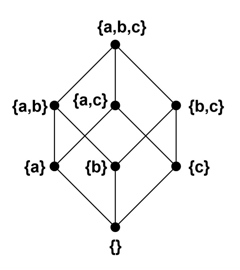
Current
Note has been deleted
Field-by-field Comparison
| Field | Before | After |
|---|---|---|
| Front | ||
| Back |
Note 948: ETH::1. Semester::DiskMat
Deck: ETH::1. Semester::DiskMat
Note Type: Horvath Classic
GUID:
deleted
Note Type: Horvath Classic
GUID:
v2<,m(`1YY
Deleted Note
Front
When are two elements \(a\) and \(b\) comparable in a poset \((A; \preceq)\)?
Back
When are two elements \(a\) and \(b\) comparable in a poset \((A; \preceq)\)?
When \(a \preceq b\) or \(b \preceq a\). Otherwise they are incomparable.
Current
Note has been deleted
Field-by-field Comparison
| Field | Before | After |
|---|---|---|
| Front | ||
| Back |
Note 949: ETH::1. Semester::DiskMat
Deck: ETH::1. Semester::DiskMat
Note Type: Horvath Classic
GUID:
deleted
Note Type: Horvath Classic
GUID:
v9=<1hp!B8
Deleted Note
Front
What is a zerodivisor?
Back
What is a zerodivisor?
A zerodivisor \(a \in R, a \neq 0\) in a commutative ring such that \(ab = ba = 0\) for \(b \neq 0\).
Current
Note has been deleted
Field-by-field Comparison
| Field | Before | After |
|---|---|---|
| Front | ||
| Back |
Note 950: ETH::1. Semester::DiskMat
Deck: ETH::1. Semester::DiskMat
Note Type: Horvath Cloze
GUID:
deleted
Note Type: Horvath Cloze
GUID:
v
Deleted Note
Front
What two properties must a relation \(f: A \to B\) have to be a function?
- Total-definedness: \(\forall a \in A \ \exists b \in B : a \ f \ b\)
- Well-definedness: \(\forall a \in A \ \forall b, b' \in B : (a \ f \ b \land a \ f \ b' \rightarrow b = b')\)
Back
What two properties must a relation \(f: A \to B\) have to be a function?
- Total-definedness: \(\forall a \in A \ \exists b \in B : a \ f \ b\)
- Well-definedness: \(\forall a \in A \ \forall b, b' \in B : (a \ f \ b \land a \ f \ b' \rightarrow b = b')\)
Current
Note has been deleted
Field-by-field Comparison
| Field | Before | After |
|---|---|---|
| Text |
Note 951: ETH::1. Semester::DiskMat
Deck: ETH::1. Semester::DiskMat
Note Type: Horvath Classic
GUID:
deleted
Note Type: Horvath Classic
GUID:
vD12#kM5/-
Deleted Note
Front
Number of subgroups of \(\langle \mathbb{Z}_m \times \mathbb{Z}_n \rangle\)
Back
Number of subgroups of \(\langle \mathbb{Z}_m \times \mathbb{Z}_n \rangle\)
\(\sum_{a \mid m \land b \mid n} \gcd(a, b)\)
Current
Note has been deleted
Field-by-field Comparison
| Field | Before | After |
|---|---|---|
| Front | ||
| Back |
Note 952: ETH::1. Semester::DiskMat
Deck: ETH::1. Semester::DiskMat
Note Type: Horvath Classic
GUID:
deleted
Note Type: Horvath Classic
GUID:
vH;[>&}OXg
Deleted Note
Front
Conjunction
Back
Conjunction
\(\land\)
Current
Note has been deleted
Field-by-field Comparison
| Field | Before | After |
|---|---|---|
| Front | ||
| Back |
Note 953: ETH::1. Semester::DiskMat
Deck: ETH::1. Semester::DiskMat
Note Type: Horvath Classic
GUID:
deleted
Note Type: Horvath Classic
GUID:
vHNwBT2PnJ
Deleted Note
Front
What is the transitive closure \(\rho^*\) of a relation \(\rho\)?
Back
What is the transitive closure \(\rho^*\) of a relation \(\rho\)?
\[\rho^{*} = \bigcup_{n \in \mathbb{N} \setminus \{0\}} \rho^n\]
The "reachability relation" - \((a,b) \in \rho^*\) iff there's a path of finite length from \(a\) to \(b\) in \(\rho\).
Current
Note has been deleted
Field-by-field Comparison
| Field | Before | After |
|---|---|---|
| Front | ||
| Back |
Note 954: ETH::1. Semester::DiskMat
Deck: ETH::1. Semester::DiskMat
Note Type: Horvath Cloze
GUID:
deleted
Note Type: Horvath Cloze
GUID:
vKeo,n,kS
Deleted Note
Front
The group \(\langle \mathbb{Z}_n; \oplus \rangle\) is cyclic for every \(n\), where 1 is always a generator.
Back
The group \(\langle \mathbb{Z}_n; \oplus \rangle\) is cyclic for every \(n\), where 1 is always a generator.
Current
Note has been deleted
Field-by-field Comparison
| Field | Before | After |
|---|---|---|
| Text |
Note 955: ETH::1. Semester::DiskMat
Deck: ETH::1. Semester::DiskMat
Note Type: Horvath Cloze
GUID:
deleted
Note Type: Horvath Cloze
GUID:
vRto[%;el{
Deleted Note
Front
The smallest subgroup of a group \(G\) containing \(a \in G\) is the group generated by \(a\), \(\langle a \rangle\).
Back
The smallest subgroup of a group \(G\) containing \(a \in G\) is the group generated by \(a\), \(\langle a \rangle\).
Current
Note has been deleted
Field-by-field Comparison
| Field | Before | After |
|---|---|---|
| Text |
Note 956: ETH::1. Semester::DiskMat
Deck: ETH::1. Semester::DiskMat
Note Type: Horvath Cloze
GUID:
deleted
Note Type: Horvath Cloze
GUID:
v[{@yotn>*
Deleted Note
Front
In a field F, \(y \in F\) is a root of \(a(x)\) if and only if \(x - y\) divides \(a(x)\) or \(a(y) = 0\)
Back
In a field F, \(y \in F\) is a root of \(a(x)\) if and only if \(x - y\) divides \(a(x)\) or \(a(y) = 0\)
Current
Note has been deleted
Field-by-field Comparison
| Field | Before | After |
|---|---|---|
| Text |
Note 957: ETH::1. Semester::DiskMat
Deck: ETH::1. Semester::DiskMat
Note Type: Horvath Classic
GUID:
deleted
Note Type: Horvath Classic
GUID:
v]O5De@N,S
Deleted Note
Front
How is the GCD related to ideals? (Lemma 4.4)
Back
How is the GCD related to ideals? (Lemma 4.4)
Let \(a, b \in \mathbb{Z}\) (not both 0).
If \((a, b) = (d)\), then \(d\) is a greatest common divisor of \(a\) and \(b\).
If \((a, b) = (d)\), then \(d\) is a greatest common divisor of \(a\) and \(b\).
Current
Note has been deleted
Field-by-field Comparison
| Field | Before | After |
|---|---|---|
| Front | ||
| Back |
Note 958: ETH::1. Semester::DiskMat
Deck: ETH::1. Semester::DiskMat
Note Type: Horvath Cloze
GUID:
deleted
Note Type: Horvath Cloze
GUID:
vi7xPhAi#`
Deleted Note
Front
If \(e * a = a * e = a\) for all \(a \in S\), then \(e\) is simply called a neutral element or identity element.
Back
If \(e * a = a * e = a\) for all \(a \in S\), then \(e\) is simply called a neutral element or identity element.
Current
Note has been deleted
Field-by-field Comparison
| Field | Before | After |
|---|---|---|
| Text |
Note 959: ETH::1. Semester::DiskMat
Deck: ETH::1. Semester::DiskMat
Note Type: Horvath Cloze
GUID:
deleted
Note Type: Horvath Cloze
GUID:
vnO
Deleted Note
Front
Equivalence relation is a relation on a set \(A\) that is
* reflexive
* symmetric
* transitive
Back
Equivalence relation is a relation on a set \(A\) that is
* reflexive
* symmetric
* transitive
Example: \(\equiv_m \)
Current
Note has been deleted
Field-by-field Comparison
| Field | Before | After |
|---|---|---|
| Text | ||
| Extra |
Note 960: ETH::1. Semester::DiskMat
Deck: ETH::1. Semester::DiskMat
Note Type: Horvath Cloze
GUID:
deleted
Note Type: Horvath Cloze
GUID:
vpgCC{U)O3
Deleted Note
Front
A cyclic group of order \(n\) {{c1::is isomorphic to \(\langle \mathbb{Z}_n,\oplus)\), and hence commutative.::has which useful property?}}
Back
A cyclic group of order \(n\) {{c1::is isomorphic to \(\langle \mathbb{Z}_n,\oplus)\), and hence commutative.::has which useful property?}}
Current
Note has been deleted
Field-by-field Comparison
| Field | Before | After |
|---|---|---|
| Text |
Note 961: ETH::1. Semester::DiskMat
Deck: ETH::1. Semester::DiskMat
Note Type: Horvath Cloze
GUID:
deleted
Note Type: Horvath Cloze
GUID:
vt:Wqzxx@@
Deleted Note
Front
A subgroup \(H\) of a group \(G\) is a subset \(H \subseteq G\) which is a group in itself (closed with respect to all operations, includes neutral element, inverses exist).
Back
A subgroup \(H\) of a group \(G\) is a subset \(H \subseteq G\) which is a group in itself (closed with respect to all operations, includes neutral element, inverses exist).
Trivial subgroups: \(\{e\}, G\)
Current
Note has been deleted
Field-by-field Comparison
| Field | Before | After |
|---|---|---|
| Text | ||
| Extra |
Note 962: ETH::1. Semester::DiskMat
Deck: ETH::1. Semester::DiskMat
Note Type: Horvath Classic
GUID:
deleted
Note Type: Horvath Classic
GUID:
vx[#sC8q?V
Deleted Note
Front
What property does every finite field \(\text{GF}(q)\) have (and what does \(q\) satisfy)?
Back
What property does every finite field \(\text{GF}(q)\) have (and what does \(q\) satisfy)?
Theorem 5.40: The multiplicative group of every finite field \(\text{GF}(q)\) is cyclic (as \(q\) is a power of a prime, if \(\text{GF}(q)\) is cyclic).
This group has order \(q - 1\) and \(\varphi(q-1)\) generators.
Note that even though q is not prime thus not every integer is coprime, GF(q) is not Z_q.
Current
Note has been deleted
Field-by-field Comparison
| Field | Before | After |
|---|---|---|
| Front | ||
| Back |
Note 963: ETH::1. Semester::DiskMat
Deck: ETH::1. Semester::DiskMat
Note Type: Horvath Classic
GUID:
deleted
Note Type: Horvath Classic
GUID:
w%|YnPf>o2
Deleted Note
Front
When is a poset \((A; \preceq)\) totally ordered (linearly ordered)?
Back
When is a poset \((A; \preceq)\) totally ordered (linearly ordered)?
When any two elements of \(A\) are comparable.
Current
Note has been deleted
Field-by-field Comparison
| Field | Before | After |
|---|---|---|
| Front | ||
| Back |
Note 964: ETH::1. Semester::DiskMat
Deck: ETH::1. Semester::DiskMat
Note Type: Horvath Cloze
GUID:
deleted
Note Type: Horvath Cloze
GUID:
w99%AgTdDZ
Deleted Note
Front
Rectified form:
- no variable occurs both as a bound and as a free variable
- all quantifiers use distinct variable names
Back
Rectified form:
- no variable occurs both as a bound and as a free variable
- all quantifiers use distinct variable names
Current
Note has been deleted
Field-by-field Comparison
| Field | Before | After |
|---|---|---|
| Text |
Note 965: ETH::1. Semester::DiskMat
Deck: ETH::1. Semester::DiskMat
Note Type: Horvath Classic
GUID:
deleted
Note Type: Horvath Classic
GUID:
wJ,ON3lFCv
Deleted Note
Front
Give an example of an extension field constructed from polynomials.
Back
Give an example of an extension field constructed from polynomials.
\(\mathbb{R}[x]_{x^2+1}\) is a field, isomorphic to \(\mathbb{C}\) (the complex numbers).
Explanation: \(x^2 + 1\) is irreducible over \(\mathbb{R}\) (no real roots). Elements of \(\mathbb{R}[x]_{x^2+1}\) are of the form \(a + bx\) where \(x^2 = -1\), which corresponds exactly to complex numbers \(a + bi\).
Every proper finite extension field of \(\mathbb{R}\) is isomorphic to \(\mathbb{C}\).
Current
Note has been deleted
Field-by-field Comparison
| Field | Before | After |
|---|---|---|
| Front | ||
| Back |
Note 966: ETH::1. Semester::DiskMat
Deck: ETH::1. Semester::DiskMat
Note Type: Horvath Cloze
GUID:
deleted
Note Type: Horvath Cloze
GUID:
wJPBh5aLN<
Deleted Note
Front
\(F[x]^*_{(m(x))}\) is a field.
Back
\(F[x]^*_{(m(x))}\) is a field.
Current
Note has been deleted
Field-by-field Comparison
| Field | Before | After |
|---|---|---|
| Text |
Note 967: ETH::1. Semester::DiskMat
Deck: ETH::1. Semester::DiskMat
Note Type: Horvath Cloze
GUID:
deleted
Note Type: Horvath Cloze
GUID:
wN=e)I[rpJ
Deleted Note
Front
Every polynomial of degree 1 is irreducible.
Back
Every polynomial of degree 1 is irreducible.
Current
Note has been deleted
Field-by-field Comparison
| Field | Before | After |
|---|---|---|
| Text |
Note 968: ETH::1. Semester::DiskMat
Deck: ETH::1. Semester::DiskMat
Note Type: Horvath Classic
GUID:
deleted
Note Type: Horvath Classic
GUID:
wV8=4Xrwg1
Deleted Note
Front
\(F[x]_{m(x)}^*\) is defined as:
Back
\(F[x]_{m(x)}^*\) is defined as:
\[\{ a(x) \in F[x]_{m(x)} \ | \ \gcd(a(x), m(x)) = 1 \}\]
Current
Note has been deleted
Field-by-field Comparison
| Field | Before | After |
|---|---|---|
| Front | ||
| Back |
Note 969: ETH::1. Semester::DiskMat
Deck: ETH::1. Semester::DiskMat
Note Type: Horvath Cloze
GUID:
deleted
Note Type: Horvath Cloze
GUID:
wV8Y&j0xY.
Deleted Note
Front
Name the binding strengths of PL tokens in order:
- unary operators (NOT)
- quantifiers (for all and exists)
- operators (AND, OR)
- Implication
Back
Name the binding strengths of PL tokens in order:
- unary operators (NOT)
- quantifiers (for all and exists)
- operators (AND, OR)
- Implication
Current
Note has been deleted
Field-by-field Comparison
| Field | Before | After |
|---|---|---|
| Text |
Note 970: ETH::1. Semester::DiskMat
Deck: ETH::1. Semester::DiskMat
Note Type: Horvath Classic
GUID:
deleted
Note Type: Horvath Classic
GUID:
wY#5P^[
Deleted Note
Front
State Lemma 5.20 about division in integral domains: (The quotient has what property?)
Back
State Lemma 5.20 about division in integral domains: (The quotient has what property?)
Lemma 5.20: In an integral domain, if \(a \mid b\) (i.e., \(b = ac\) for some \(c\)), then \(c\) is unique and is denoted by \(c = b/a\) (the quotient).
Explanation: If \(b = ac_1\) and \(b = ac_2\), then \(a(c_1 - c_2) = 0\). Since \(a \neq 0\) in an integral domain, we must have \(c_1 - c_2 = 0\)\(\implies c_1 = c_2\).
Current
Note has been deleted
Field-by-field Comparison
| Field | Before | After |
|---|---|---|
| Front | ||
| Back |
Note 971: ETH::1. Semester::DiskMat
Deck: ETH::1. Semester::DiskMat
Note Type: Horvath Classic
GUID:
deleted
Note Type: Horvath Classic
GUID:
wv2_);uy$2
Deleted Note
Front
When is \(a \in A\) a lower bound of subset \(S \subseteq A\) in poset \((A; \preceq)\)?
Back
When is \(a \in A\) a lower bound of subset \(S \subseteq A\) in poset \((A; \preceq)\)?
When \(a \preceq b\) for all \(b \in S\).
Current
Note has been deleted
Field-by-field Comparison
| Field | Before | After |
|---|---|---|
| Front | ||
| Back |
Note 972: ETH::1. Semester::DiskMat
Deck: ETH::1. Semester::DiskMat
Note Type: Horvath Cloze
GUID:
deleted
Note Type: Horvath Cloze
GUID:
wxOSFQju/Y
Deleted Note
Front
For any prime \(p\), the Euler totient function \(\varphi(p)\) is equal to \(p-1\).
Back
For any prime \(p\), the Euler totient function \(\varphi(p)\) is equal to \(p-1\).
Current
Note has been deleted
Field-by-field Comparison
| Field | Before | After |
|---|---|---|
| Text |
Note 973: ETH::1. Semester::DiskMat
Deck: ETH::1. Semester::DiskMat
Note Type: Horvath Classic
GUID:
deleted
Note Type: Horvath Classic
GUID:
x-z%Jc>A>g
Deleted Note
Front
How does the GCD change when we subtract a multiple? (Lemma 4.2)
Back
How does the GCD change when we subtract a multiple? (Lemma 4.2)
Not at all.
For any integers \(m, n\) and \(q\): \[\text{gcd}(m, n - qm) = \text{gcd}(m, n)\] This is the key property for Euclid's algorithm: \[\text{gcd}(m, R_m(n)) = \text{gcd}(m, n)\]
For any integers \(m, n\) and \(q\): \[\text{gcd}(m, n - qm) = \text{gcd}(m, n)\] This is the key property for Euclid's algorithm: \[\text{gcd}(m, R_m(n)) = \text{gcd}(m, n)\]
Current
Note has been deleted
Field-by-field Comparison
| Field | Before | After |
|---|---|---|
| Front | ||
| Back |
Note 974: ETH::1. Semester::DiskMat
Deck: ETH::1. Semester::DiskMat
Note Type: Horvath Cloze
GUID:
deleted
Note Type: Horvath Cloze
GUID:
x/&wX)sTYn
Deleted Note
Front
An algebra (also: algebraic structure, \( \Omega\)-algebra) is a pair \(\langle S, \Omega \rangle\) where S is a set and \(\Omega = (\omega_1, \ldots, \omega_n)\) is a list of operations on S.
Back
An algebra (also: algebraic structure, \( \Omega\)-algebra) is a pair \(\langle S, \Omega \rangle\) where S is a set and \(\Omega = (\omega_1, \ldots, \omega_n)\) is a list of operations on S.
Current
Note has been deleted
Field-by-field Comparison
| Field | Before | After |
|---|---|---|
| Text |
Note 975: ETH::1. Semester::DiskMat
Deck: ETH::1. Semester::DiskMat
Note Type: Horvath Classic
GUID:
deleted
Note Type: Horvath Classic
GUID:
x9H_WtVg+E
Deleted Note
Front
Is function composition associative?
Back
Is function composition associative?
Yes: \((h \circ g) \circ f = h \circ (g \circ f)\)
Current
Note has been deleted
Field-by-field Comparison
| Field | Before | After |
|---|---|---|
| Front | ||
| Back |
Note 976: ETH::1. Semester::DiskMat
Deck: ETH::1. Semester::DiskMat
Note Type: Horvath Classic
GUID:
deleted
Note Type: Horvath Classic
GUID:
x9yn[)SlRq
Deleted Note
Front
What is the cardinality of \(A \times B\) for finite sets?
Back
What is the cardinality of \(A \times B\) for finite sets?
\(|A \times B| = |A| \cdot |B|\)
Current
Note has been deleted
Field-by-field Comparison
| Field | Before | After |
|---|---|---|
| Front | ||
| Back |
Note 977: ETH::1. Semester::DiskMat
Deck: ETH::1. Semester::DiskMat
Note Type: Horvath Cloze
GUID:
deleted
Note Type: Horvath Cloze
GUID:
xDDC{82KOB
Deleted Note
Front
Proof method: Proof by Contradiction
1. Find a suitable statement \( T\).
1. Find a suitable statement \( T\).
2. Prove that \( T \) is false.
3. Assume that \( S \) is false and prove that \( T \) is true (-> contradiction).
Back
Proof method: Proof by Contradiction
1. Find a suitable statement \( T\).
1. Find a suitable statement \( T\).
2. Prove that \( T \) is false.
3. Assume that \( S \) is false and prove that \( T \) is true (-> contradiction).
Current
Note has been deleted
Field-by-field Comparison
| Field | Before | After |
|---|---|---|
| Text |
Note 978: ETH::1. Semester::DiskMat
Deck: ETH::1. Semester::DiskMat
Note Type: Horvath Cloze
GUID:
deleted
Note Type: Horvath Cloze
GUID:
xH`d$W-97_
Deleted Note
Front
In a Group:
\(\widehat{(\widehat{a})} =\) \(a\) (inverse of inverse is the original element).
Back
In a Group:
\(\widehat{(\widehat{a})} =\) \(a\) (inverse of inverse is the original element).
This is a property from Lemma 5.3.
Current
Note has been deleted
Field-by-field Comparison
| Field | Before | After |
|---|---|---|
| Text | ||
| Extra |
Note 979: ETH::1. Semester::DiskMat
Deck: ETH::1. Semester::DiskMat
Note Type: Horvath Cloze
GUID:
deleted
Note Type: Horvath Cloze
GUID:
xWhw%ncc|4
Deleted Note
Front
Verify that \(\equiv_m\) is reflexive, symmetric, and transitive.
- Reflexive: \(a \equiv_m a\) since \(m \mid (a - a) = 0\) ✓
- Symmetric: \(a \equiv_m b \Rightarrow m \mid (a-b) \Rightarrow m \mid (b-a) \Rightarrow b \equiv_m a\) ✓
- Transitive: If \(m \mid (a-b)\) and \(m \mid (b-c)\), then \(m \mid (a-b+b-c) = (a-c)\) ✓
Back
Verify that \(\equiv_m\) is reflexive, symmetric, and transitive.
- Reflexive: \(a \equiv_m a\) since \(m \mid (a - a) = 0\) ✓
- Symmetric: \(a \equiv_m b \Rightarrow m \mid (a-b) \Rightarrow m \mid (b-a) \Rightarrow b \equiv_m a\) ✓
- Transitive: If \(m \mid (a-b)\) and \(m \mid (b-c)\), then \(m \mid (a-b+b-c) = (a-c)\) ✓
Current
Note has been deleted
Field-by-field Comparison
| Field | Before | After |
|---|---|---|
| Text |
Note 980: ETH::1. Semester::DiskMat
Deck: ETH::1. Semester::DiskMat
Note Type: Horvath Classic
GUID:
deleted
Note Type: Horvath Classic
GUID:
xZLvO#5j~[
Deleted Note
Front
When does element \(b\) cover element \(a\) in a poset \((A; \preceq)\)?
Back
When does element \(b\) cover element \(a\) in a poset \((A; \preceq)\)?
When \(a \prec b\) and there exists no \(c\) with \(a \prec c \prec b\) (i.e., \(b\) is the direct successor of \(a\)).
Current
Note has been deleted
Field-by-field Comparison
| Field | Before | After |
|---|---|---|
| Front | ||
| Back |
Note 981: ETH::1. Semester::DiskMat
Deck: ETH::1. Semester::DiskMat
Note Type: Horvath Classic
GUID:
deleted
Note Type: Horvath Classic
GUID:
x^Wv3;n[%Q
Deleted Note
Front
What is the equivalence class \([a]_\theta\) of element \(a\) under equivalence relation \(\theta\)?
Back
What is the equivalence class \([a]_\theta\) of element \(a\) under equivalence relation \(\theta\)?
\[[a]_{\theta} \overset{\text{def}}{=} \{b \in A \ | \ b \ \theta \ a\}\]
The set of all elements equivalent to \(a\).
Current
Note has been deleted
Field-by-field Comparison
| Field | Before | After |
|---|---|---|
| Front | ||
| Back |
Note 982: ETH::1. Semester::DiskMat
Deck: ETH::1. Semester::DiskMat
Note Type: Horvath Classic
GUID:
deleted
Note Type: Horvath Classic
GUID:
x`!R>+ily=
Deleted Note
Front
What is a lattice?
Back
What is a lattice?
A poset \((A; \preceq)\) in which every pair of elements has a meet and join.
Current
Note has been deleted
Field-by-field Comparison
| Field | Before | After |
|---|---|---|
| Front | ||
| Back |
Note 983: ETH::1. Semester::DiskMat
Deck: ETH::1. Semester::DiskMat
Note Type: Horvath Cloze
GUID:
deleted
Note Type: Horvath Cloze
GUID:
xelDz|Gp*?
Deleted Note
Front
A right (left) neutral element is an element such that for all \(a \in G\), \(a*e = a\) (\(e*a = a\)).
Back
A right (left) neutral element is an element such that for all \(a \in G\), \(a*e = a\) (\(e*a = a\)).
Current
Note has been deleted
Field-by-field Comparison
| Field | Before | After |
|---|---|---|
| Text |
Note 984: ETH::1. Semester::DiskMat
Deck: ETH::1. Semester::DiskMat
Note Type: Horvath Classic
GUID:
deleted
Note Type: Horvath Classic
GUID:
xkr{;Hl0wh
Deleted Note
Front
How do you find the GCD of two polynomials?
Back
How do you find the GCD of two polynomials?
To find \(\gcd(a(x), b(x))\):
- Find a common factor \((x - \alpha)\) using the roots method:
- Try all possible elements of the field to find roots
- If \(\alpha\) is a root of both, then \((x - \alpha)\) is a common factor
- Use division with remainder to reduce to smaller polynomials
- Repeat the process on the smaller polynomials
- After they have no roots anymore, try all monic polynomials up to degree d/2 to find irreducible factors.
- Important: Don't just find all roots and multiply! A root might be repeated (e.g., \((x+1)^2\)), and you'd miss the higher multiplicity
Example: For \(a(x) = (x+1)(x+1)(x+2)\), the GCD with another polynomial might be \((x+1)^2\), not just \((x+1)\).
Current
Note has been deleted
Field-by-field Comparison
| Field | Before | After |
|---|---|---|
| Front | ||
| Back |
Note 985: ETH::1. Semester::DiskMat
Deck: ETH::1. Semester::DiskMat
Note Type: Horvath Classic
GUID:
deleted
Note Type: Horvath Classic
GUID:
xp_U|[rM*4
Deleted Note
Front
List all subgroups of \(\mathbb{Z}_{12}\).
Back
List all subgroups of \(\mathbb{Z}_{12}\).
The subgroups of \(\mathbb{Z}_{12}\) are:
- \(\{0\}\) (trivial subgroup)
- \(\{0, 6\}\)
- \(\{0, 4, 8\}\)
- \(\{0, 3, 6, 9\}\)
- \(\{0, 2, 4, 6, 8, 10\}\)
- \(\mathbb{Z}_{12}\) (trivial subgroup - the whole group)
Current
Note has been deleted
Field-by-field Comparison
| Field | Before | After |
|---|---|---|
| Front | ||
| Back |
Note 986: ETH::1. Semester::DiskMat
Deck: ETH::1. Semester::DiskMat
Note Type: Horvath Cloze
GUID:
deleted
Note Type: Horvath Cloze
GUID:
y&2ryUB}aI
Deleted Note
Front
A ring \(R\) is a field if and only if {{c1:: \(\langle R \setminus \{0\}; \cdot, \text{ }^{-1}, 1 \rangle\) is an abelian group}}.
Back
A ring \(R\) is a field if and only if {{c1:: \(\langle R \setminus \{0\}; \cdot, \text{ }^{-1}, 1 \rangle\) is an abelian group}}.
Current
Note has been deleted
Field-by-field Comparison
| Field | Before | After |
|---|---|---|
| Text |
Note 987: ETH::1. Semester::DiskMat
Deck: ETH::1. Semester::DiskMat
Note Type: Horvath Classic
GUID:
deleted
Note Type: Horvath Classic
GUID:
y)
Deleted Note
Front
Proof method: "Direct Proof of an Implication"
Back
Proof method: "Direct Proof of an Implication"
Assume \(S\) and prove \(T\) under that assumption.
Current
Note has been deleted
Field-by-field Comparison
| Field | Before | After |
|---|---|---|
| Front | ||
| Back |
Note 988: ETH::1. Semester::DiskMat
Deck: ETH::1. Semester::DiskMat
Note Type: Horvath Classic
GUID:
deleted
Note Type: Horvath Classic
GUID:
y+%Du@ss=x
Deleted Note
Front
If we intersect two equivalence relations, what do we get?
Back
If we intersect two equivalence relations, what do we get?
Another equivalence relation.
Current
Note has been deleted
Field-by-field Comparison
| Field | Before | After |
|---|---|---|
| Front | ||
| Back |
Note 989: ETH::1. Semester::DiskMat
Deck: ETH::1. Semester::DiskMat
Note Type: Horvath Classic
GUID:
deleted
Note Type: Horvath Classic
GUID:
y+DFM]G]@{
Deleted Note
Front
Proof method: Existence Proof
Back
Proof method: Existence Proof
We just want to prove that there exists a \( x \) such that a statement \( S_x \) is true. (e.g. There exists a prime number such that \( n - 10\) and \( n + 10\) are also prime.)
constructive: We know the x.
non-constructive: We know that x has to exist, but we don't know its value.
Current
Note has been deleted
Field-by-field Comparison
| Field | Before | After |
|---|---|---|
| Front | ||
| Back |
Note 990: ETH::1. Semester::DiskMat
Deck: ETH::1. Semester::DiskMat
Note Type: Horvath Classic
GUID:
deleted
Note Type: Horvath Classic
GUID:
y,yASV&n3a
Deleted Note
Front
What kind of relation is equinumerosity (\(\sim\))?
Back
What kind of relation is equinumerosity (\(\sim\))?
The relation \(\sim\) (equinumerous) is an equivalence relation.
(It is reflexive, symmetric, and transitive)
(It is reflexive, symmetric, and transitive)
Current
Note has been deleted
Field-by-field Comparison
| Field | Before | After |
|---|---|---|
| Front | ||
| Back |
Note 991: ETH::1. Semester::DiskMat
Deck: ETH::1. Semester::DiskMat
Note Type: Horvath Cloze
GUID:
deleted
Note Type: Horvath Cloze
GUID:
y4s0XCy@A
Deleted Note
Front
Consider the poset \((A; \preceq)\).
\(a \in A\) is the least (greatest) element of \(A\) if \(a \preceq b\) (\(a \succeq b) \) for all \(b \in A\)
Back
Consider the poset \((A; \preceq)\).
\(a \in A\) is the least (greatest) element of \(A\) if \(a \preceq b\) (\(a \succeq b) \) for all \(b \in A\)
Note that a least or a greatest element need not exist. However, there can be at most one least element, as suggested by the word “the” in the definition.
This follows directly from the antisymmetry of \(\preceq\). If there were two least elements, they would be mutually comparable, and hence must be equal.
This follows directly from the antisymmetry of \(\preceq\). If there were two least elements, they would be mutually comparable, and hence must be equal.
Current
Note has been deleted
Field-by-field Comparison
| Field | Before | After |
|---|---|---|
| Text | ||
| Extra |
Note 992: ETH::1. Semester::DiskMat
Deck: ETH::1. Semester::DiskMat
Note Type: Horvath Classic
GUID:
deleted
Note Type: Horvath Classic
GUID:
y7i@2u]aPf
Deleted Note
Front
What properties does the relation \(=\) satisfy?
Back
What properties does the relation \(=\) satisfy?
- Reflexivity
- Symmetry
- Antisymmetry
- Transitivity
Thus, it's both an equivalence and a partial order relation!
Current
Note has been deleted
Field-by-field Comparison
| Field | Before | After |
|---|---|---|
| Front | ||
| Back |
Note 993: ETH::1. Semester::DiskMat
Deck: ETH::1. Semester::DiskMat
Note Type: Horvath Classic
GUID:
deleted
Note Type: Horvath Classic
GUID:
y;`2Cs<0nK
Deleted Note
Front
What is the modus ponens logical rule?
Back
What is the modus ponens logical rule?
\(A \land (A \rightarrow B) \models B\)
(If \(A\) is true and \(A\) implies \(B\), then \(B\) is true)
(If \(A\) is true and \(A\) implies \(B\), then \(B\) is true)
Current
Note has been deleted
Field-by-field Comparison
| Field | Before | After |
|---|---|---|
| Front | ||
| Back |
Note 994: ETH::1. Semester::DiskMat
Deck: ETH::1. Semester::DiskMat
Note Type: Horvath Cloze
GUID:
deleted
Note Type: Horvath Cloze
GUID:
yAP=DE#~t<
Deleted Note
Front
An abelian group has the following properties:
- Closure
- Associativity
- Identity
- Inverse
- Commutativity
Back
An abelian group has the following properties:
- Closure
- Associativity
- Identity
- Inverse
- Commutativity
Current
Note has been deleted
Field-by-field Comparison
| Field | Before | After |
|---|---|---|
| Text |
Note 995: ETH::1. Semester::DiskMat
Deck: ETH::1. Semester::DiskMat
Note Type: Horvath Classic
GUID:
deleted
Note Type: Horvath Classic
GUID:
yBtcC{e:]{
Deleted Note
Front
What does it mean for a set \(A\) to be countable?
Back
What does it mean for a set \(A\) to be countable?
\(A \preceq \mathbb{N}\) (i.e., there exists an injection \(A \to \mathbb{N}\))
Current
Note has been deleted
Field-by-field Comparison
| Field | Before | After |
|---|---|---|
| Front | ||
| Back |
Note 996: ETH::1. Semester::DiskMat
Deck: ETH::1. Semester::DiskMat
Note Type: Horvath Cloze
GUID:
deleted
Note Type: Horvath Cloze
GUID:
yF7brLJQxE
Deleted Note
Front
Consider the poset \((A; \preceq)\) and \( S \subseteq A\).
\(a \in A\) is the greatest lower (least upper) bound of \(S\) if \(a\) is the greatest (least) element of the set of all lower (upper) bounds of \(S\).
Back
Consider the poset \((A; \preceq)\) and \( S \subseteq A\).
\(a \in A\) is the greatest lower (least upper) bound of \(S\) if \(a\) is the greatest (least) element of the set of all lower (upper) bounds of \(S\).
Note that greatest (least) refers to the operation \(\preceq\) and not to order by \(>\) or \(<\) (smaller, bigger).
Current
Note has been deleted
Field-by-field Comparison
| Field | Before | After |
|---|---|---|
| Text | ||
| Extra |
Note 997: ETH::1. Semester::DiskMat
Deck: ETH::1. Semester::DiskMat
Note Type: Horvath Cloze
GUID:
deleted
Note Type: Horvath Cloze
GUID:
yIRK71/G/r
Deleted Note
Front
A mathematical statement not known, but believed, to be true or false is called a conjecture.
Back
A mathematical statement not known, but believed, to be true or false is called a conjecture.
Example: Collatz conjecture.
Current
Note has been deleted
Field-by-field Comparison
| Field | Before | After |
|---|---|---|
| Text | ||
| Extra |
Note 998: ETH::1. Semester::DiskMat
Deck: ETH::1. Semester::DiskMat
Note Type: Horvath Cloze
GUID:
deleted
Note Type: Horvath Cloze
GUID:
yJ}kX&Y9Od
Deleted Note
Front
A relation ρ on a set A is called symmetric if {{c2::\( a \ \rho \ b \iff b \ \rho \ a\) is true, i.e. if \( \rho = \hat{\rho}\)}}
Back
A relation ρ on a set A is called symmetric if {{c2::\( a \ \rho \ b \iff b \ \rho \ a\) is true, i.e. if \( \rho = \hat{\rho}\)}}
Examples: \( \equiv_m\), marriage
Current
Note has been deleted
Field-by-field Comparison
| Field | Before | After |
|---|---|---|
| Text | ||
| Extra |
Note 999: ETH::1. Semester::DiskMat
Deck: ETH::1. Semester::DiskMat
Note Type: Horvath Cloze
GUID:
deleted
Note Type: Horvath Cloze
GUID:
yK:4+{Du_V
Deleted Note
Front
A codeword \(c\) of length \(n\) in a polynomial code with degree \(k-1\) can be interpolated from any \(k\) values by Lagrangian interpolation.
Back
A codeword \(c\) of length \(n\) in a polynomial code with degree \(k-1\) can be interpolated from any \(k\) values by Lagrangian interpolation.
Current
Note has been deleted
Field-by-field Comparison
| Field | Before | After |
|---|---|---|
| Text |
Note 1000: ETH::1. Semester::DiskMat
Deck: ETH::1. Semester::DiskMat
Note Type: Horvath Classic
GUID:
deleted
Note Type: Horvath Classic
GUID:
yYxXL_?YQ>
Deleted Note
Front
Why does the Chinese Remainder Theorem require \(m_1, \dots, m_r\) to be pairwise relatively prime?
Back
Why does the Chinese Remainder Theorem require \(m_1, \dots, m_r\) to be pairwise relatively prime?
If \(\text{gcd}(m_i, m_j) = d > 1\), then the system could be inconsistent (e.g., \(x \equiv 0 \pmod{6}\) and \(x \equiv 1 \pmod{4}\) has no solution) or have multiple solutions (destroying uniqueness).
Current
Note has been deleted
Field-by-field Comparison
| Field | Before | After |
|---|---|---|
| Front | ||
| Back |
Note 1001: ETH::1. Semester::DiskMat
Deck: ETH::1. Semester::DiskMat
Note Type: Horvath Cloze
GUID:
deleted
Note Type: Horvath Cloze
GUID:
y`5($Q$d37
Deleted Note
Front
Eine Gruppe ist eine Menge \(G\) mit Operation \( * \) mit folgenden Eigenschaften:
- {{c2::
- Assoziativität: \((a * b) * c = a * (b*c)\)
- Neutrales Element existiert: \( a * e = e * a = a \)
- Jedes Element \(a\in G\) hat eine Inverse: \( a * a^{-1} = a^{-1} * a = e\) }}
Back
Eine Gruppe ist eine Menge \(G\) mit Operation \( * \) mit folgenden Eigenschaften:
- {{c2::
- Assoziativität: \((a * b) * c = a * (b*c)\)
- Neutrales Element existiert: \( a * e = e * a = a \)
- Jedes Element \(a\in G\) hat eine Inverse: \( a * a^{-1} = a^{-1} * a = e\) }}
Current
Note has been deleted
Field-by-field Comparison
| Field | Before | After |
|---|---|---|
| Text |
Note 1002: ETH::1. Semester::DiskMat
Deck: ETH::1. Semester::DiskMat
Note Type: Horvath Cloze
GUID:
deleted
Note Type: Horvath Cloze
GUID:
ykM`*q&]Lu
Deleted Note
Front
\(F \equiv G\) means F and G are equivalent, i.e., their truth values are equal for all truth assignments to the propositional symbols appearing in \(F\) or \(G\).
Back
\(F \equiv G\) means F and G are equivalent, i.e., their truth values are equal for all truth assignments to the propositional symbols appearing in \(F\) or \(G\).
Current
Note has been deleted
Field-by-field Comparison
| Field | Before | After |
|---|---|---|
| Text |
Note 1003: ETH::1. Semester::DiskMat
Deck: ETH::1. Semester::DiskMat
Note Type: Horvath Classic
GUID:
deleted
Note Type: Horvath Classic
GUID:
yl]2udZDYh
Deleted Note
Front
What is a binary relation from set \(A\) to set \(B\)?
Back
What is a binary relation from set \(A\) to set \(B\)?
A subset of \(A \times B\). If \(A = B\), then \(\rho\) is called a relation on \(A\).
Current
Note has been deleted
Field-by-field Comparison
| Field | Before | After |
|---|---|---|
| Front | ||
| Back |
Note 1004: ETH::1. Semester::DiskMat
Deck: ETH::1. Semester::DiskMat
Note Type: Horvath Cloze
GUID:
deleted
Note Type: Horvath Cloze
GUID:
ymyo>YcM?L
Deleted Note
Front
If \(D\) is an integral domain, then \(D[x]\) also is an integral domain.
Back
If \(D\) is an integral domain, then \(D[x]\) also is an integral domain.
Lemma 5.22(1)
Current
Note has been deleted
Field-by-field Comparison
| Field | Before | After |
|---|---|---|
| Text | ||
| Extra |
Note 1005: ETH::1. Semester::DiskMat
Deck: ETH::1. Semester::DiskMat
Note Type: Horvath Classic
GUID:
deleted
Note Type: Horvath Classic
GUID:
yvfeO9PXGk
Deleted Note
Front
How does symmetry of a relation appear in matrix representation?
Back
How does symmetry of a relation appear in matrix representation?
The matrix is symmetric (equals its own transpose).
Current
Note has been deleted
Field-by-field Comparison
| Field | Before | After |
|---|---|---|
| Front | ||
| Back |
Note 1006: ETH::1. Semester::DiskMat
Deck: ETH::1. Semester::DiskMat
Note Type: Horvath Classic
GUID:
deleted
Note Type: Horvath Classic
GUID:
y|z>._M[it
Deleted Note
Front
An integral domain has the following properties:
Back
An integral domain has the following properties:
Additive Group:
- closure
- associativity
- identity
- inverse
- commutative
Multiplicative group:
- closure
- associativity
- distributivity
- identity
- commutative
- no zero-divisors
Current
Note has been deleted
Field-by-field Comparison
| Field | Before | After |
|---|---|---|
| Front | ||
| Back |
Note 1007: ETH::1. Semester::DiskMat
Deck: ETH::1. Semester::DiskMat
Note Type: Horvath Classic
GUID:
deleted
Note Type: Horvath Classic
GUID:
z&#Z_j.A(t
Deleted Note
Front
What is the definition of the identity relation \(\text{id}_A\) on set \(A\)?
Back
What is the definition of the identity relation \(\text{id}_A\) on set \(A\)?
\[\text{id}_A = \{(a, a) \ | \ a \in A\}\]
Current
Note has been deleted
Field-by-field Comparison
| Field | Before | After |
|---|---|---|
| Front | ||
| Back |
Note 1008: ETH::1. Semester::DiskMat
Deck: ETH::1. Semester::DiskMat
Note Type: Horvath Classic
GUID:
deleted
Note Type: Horvath Classic
GUID:
z(I@k-aq<%
Deleted Note
Front
Why is \((\mathbb{N}; |)\) NOT totally ordered?
Back
Why is \((\mathbb{N}; |)\) NOT totally ordered?
Because \(2 \nmid 3\) and \(3 \nmid 2\) (they are incomparable).
Current
Note has been deleted
Field-by-field Comparison
| Field | Before | After |
|---|---|---|
| Front | ||
| Back |
Note 1009: ETH::1. Semester::DiskMat
Deck: ETH::1. Semester::DiskMat
Note Type: Horvath Cloze
GUID:
deleted
Note Type: Horvath Cloze
GUID:
z)u:>M_Ael
Deleted Note
Front
The {{c2::output \((c_0, \dots, c_{n-1})\)}} of an encoding function is called a codeword.
Back
The {{c2::output \((c_0, \dots, c_{n-1})\)}} of an encoding function is called a codeword.
Current
Note has been deleted
Field-by-field Comparison
| Field | Before | After |
|---|---|---|
| Text |
Note 1010: ETH::1. Semester::DiskMat
Deck: ETH::1. Semester::DiskMat
Note Type: Horvath Cloze
GUID:
deleted
Note Type: Horvath Cloze
GUID:
z8F6Pa3U/=
Deleted Note
Front
A \(k\)-ary predicate \(P\) on \(U\) is a {{c1::function \(U^k \to \{0, 1\}\)}}.
Back
A \(k\)-ary predicate \(P\) on \(U\) is a {{c1::function \(U^k \to \{0, 1\}\)}}.
Example: \(\text{prime}(x)=\begin{cases}1 & \text{if } x \text{ is prime}\\0 & \text{else}\end{cases}\)
Current
Note has been deleted
Field-by-field Comparison
| Field | Before | After |
|---|---|---|
| Text | ||
| Extra |
Note 1011: ETH::1. Semester::DiskMat
Deck: ETH::1. Semester::DiskMat
Note Type: Horvath Classic
GUID:
deleted
Note Type: Horvath Classic
GUID:
z;jp`Lcv<(
Deleted Note
Front
What is the difference between propositional and predicate logic?
Back
What is the difference between propositional and predicate logic?
propositional: only values of \(\{0,1\}\), finite
predicate: any values in our universe, infinite
Current
Note has been deleted
Field-by-field Comparison
| Field | Before | After |
|---|---|---|
| Front | ||
| Back |
Note 1012: ETH::1. Semester::DiskMat
Deck: ETH::1. Semester::DiskMat
Note Type: Horvath Classic
GUID:
deleted
Note Type: Horvath Classic
GUID:
z>oucv;uc6
Deleted Note
Front
What are both distributive laws in propositional logic?
Back
What are both distributive laws in propositional logic?
- \(A \land (B \lor C) \equiv (A \land B) \lor (A \land C)\) (distributing \(\land\) over \(\lor\))
- \(A \lor (B \land C) \equiv (A \lor B) \land (A \lor C)\) (distributing \(\lor\) over \(\land\))
Current
Note has been deleted
Field-by-field Comparison
| Field | Before | After |
|---|---|---|
| Front | ||
| Back |
Note 1013: ETH::1. Semester::DiskMat
Deck: ETH::1. Semester::DiskMat
Note Type: Horvath Classic
GUID:
deleted
Note Type: Horvath Classic
GUID:
z?HLQ7,LxY
Deleted Note
Front
Give the formal definition of subset (\(A \subseteq B\)).
Back
Give the formal definition of subset (\(A \subseteq B\)).
\[A \subseteq B \overset{\text{def}}{\Longleftrightarrow} \forall x (x \in A \rightarrow x \in B)\]
Current
Note has been deleted
Field-by-field Comparison
| Field | Before | After |
|---|---|---|
| Front | ||
| Back |
Note 1014: ETH::1. Semester::DiskMat
Deck: ETH::1. Semester::DiskMat
Note Type: Horvath Cloze
GUID:
deleted
Note Type: Horvath Cloze
GUID:
zDSrp9w@De
Deleted Note
Front
In a group, the equation \(a * x = b\) (and \(x*a = b\)) has a unique solution \(x\) for any \(a\) and \(b\).
Back
In a group, the equation \(a * x = b\) (and \(x*a = b\)) has a unique solution \(x\) for any \(a\) and \(b\).
Current
Note has been deleted
Field-by-field Comparison
| Field | Before | After |
|---|---|---|
| Text |
Note 1015: ETH::1. Semester::DiskMat
Deck: ETH::1. Semester::DiskMat
Note Type: Horvath Cloze
GUID:
deleted
Note Type: Horvath Cloze
GUID:
zK!1=,UI{i
Deleted Note
Front
All generators of {{c2:: \(\langle \mathbb{Z}_n; \oplus \rangle\)}} are coprime to \(n\).
Back
All generators of {{c2:: \(\langle \mathbb{Z}_n; \oplus \rangle\)}} are coprime to \(n\).
Current
Note has been deleted
Field-by-field Comparison
| Field | Before | After |
|---|---|---|
| Text |
Note 1016: ETH::1. Semester::DiskMat
Deck: ETH::1. Semester::DiskMat
Note Type: Horvath Classic
GUID:
deleted
Note Type: Horvath Classic
GUID:
zK&m+p6p[M
Deleted Note
Front
Give the formal definitions of union and intersection.
Back
Give the formal definitions of union and intersection.
- \(A \cup B \overset{\text{def}}{=} \{x \ | \ x \in A \lor x \in B\}\)
- \(A \cap B \overset{\text{def}}{=} \{x \ | \ x \in A \land x \in B\}\)
Current
Note has been deleted
Field-by-field Comparison
| Field | Before | After |
|---|---|---|
| Front | ||
| Back |
Note 1017: ETH::1. Semester::DiskMat
Deck: ETH::1. Semester::DiskMat
Note Type: Horvath Classic
GUID:
deleted
Note Type: Horvath Classic
GUID:
zKQ!xV
Deleted Note
Front
What fundamental property distinguishes finite from infinite sets regarding proper subsets?
Back
What fundamental property distinguishes finite from infinite sets regarding proper subsets?
A finite set never has the same cardinality as one of its proper subsets. An infinite set can (e.g., \(\mathbb{N} \sim \mathbb{O}\) where \(\mathbb{O}\) is the set of odd numbers).
Current
Note has been deleted
Field-by-field Comparison
| Field | Before | After |
|---|---|---|
| Front | ||
| Back |
Note 1018: ETH::1. Semester::DiskMat
Deck: ETH::1. Semester::DiskMat
Note Type: Horvath Cloze
GUID:
deleted
Note Type: Horvath Cloze
GUID:
zKcmqH!B|+
Deleted Note
Front
To prove \(\phi: G \rightarrow H\) is an isomorphism, you must verify two main properties:
- \(\phi\) is a homomorphism
- \(\phi\) is a bijection.
Back
To prove \(\phi: G \rightarrow H\) is an isomorphism, you must verify two main properties:
- \(\phi\) is a homomorphism
- \(\phi\) is a bijection.
Current
Note has been deleted
Field-by-field Comparison
| Field | Before | After |
|---|---|---|
| Text |
Note 1019: ETH::1. Semester::DiskMat
Deck: ETH::1. Semester::DiskMat
Note Type: Horvath Classic
GUID:
deleted
Note Type: Horvath Classic
GUID:
zRN1V|E{mK
Deleted Note
Front
Give the formal definition of composition \(\rho \circ \sigma\) where \(\rho: A \to B\) and \(\sigma: B \to C\).
Back
Give the formal definition of composition \(\rho \circ \sigma\) where \(\rho: A \to B\) and \(\sigma: B \to C\).
\[\rho \circ \sigma \overset{\text{def}}{=} \{(a, c) \ | \ \exists b ((a, b) \in \rho \land (b, c) \in \sigma)\}\]
Current
Note has been deleted
Field-by-field Comparison
| Field | Before | After |
|---|---|---|
| Front | ||
| Back |
Note 1020: ETH::1. Semester::DiskMat
Deck: ETH::1. Semester::DiskMat
Note Type: Horvath Cloze
GUID:
deleted
Note Type: Horvath Cloze
GUID:
zT<$3-%Ev[
Deleted Note
Front
We can solve \(R_a(b^c)\) by using the fact that {{c1:: \(R_a(b^c) = R_a(b^{R_{\varphi(a)}(c)})\)}} if \(a, b\) coprime.
Back
We can solve \(R_a(b^c)\) by using the fact that {{c1:: \(R_a(b^c) = R_a(b^{R_{\varphi(a)}(c)})\)}} if \(a, b\) coprime.
Note that we can't simply reduce by \(a\)!
Current
Note has been deleted
Field-by-field Comparison
| Field | Before | After |
|---|---|---|
| Text | ||
| Extra |
Note 1021: ETH::1. Semester::DiskMat
Deck: ETH::1. Semester::DiskMat
Note Type: Horvath Classic
GUID:
deleted
Note Type: Horvath Classic
GUID:
zX4AzKz1,)
Deleted Note
Front
What are the distributive laws for sets?
Back
What are the distributive laws for sets?
- \(A \cap (B \cup C) = (A \cap B) \cup (A \cap C)\)
- \(A \cup (B \cap C) = (A \cup B) \cap (A \cup C)\)
Current
Note has been deleted
Field-by-field Comparison
| Field | Before | After |
|---|---|---|
| Front | ||
| Back |
Note 1022: ETH::1. Semester::DiskMat
Deck: ETH::1. Semester::DiskMat
Note Type: Horvath Cloze
GUID:
deleted
Note Type: Horvath Cloze
GUID:
z`P{~ta];p
Deleted Note
Front
The degree of the polynomial \(0\) is defined as \(-\infty\).
Back
The degree of the polynomial \(0\) is defined as \(-\infty\).
Current
Note has been deleted
Field-by-field Comparison
| Field | Before | After |
|---|---|---|
| Text |
Note 1023: ETH::1. Semester::DiskMat
Deck: ETH::1. Semester::DiskMat
Note Type: Horvath Classic
GUID:
deleted
Note Type: Horvath Classic
GUID:
zic@0yO~I[
Deleted Note
Front
When is a field an integral domain? (Proof included)
Back
When is a field an integral domain? (Proof included)
Theorem 5.24: A field is always an integral domain.
Proof idea: If \(ab = 0\) in a field and \(a \neq 0\), then \(a\) has an inverse \(a^{-1}\). Multiplying both sides by \(a^{-1}\) gives \(b = a^{-1} \cdot 0 = 0\).
Current
Note has been deleted
Field-by-field Comparison
| Field | Before | After |
|---|---|---|
| Front | ||
| Back |
Note 1024: ETH::1. Semester::DiskMat
Deck: ETH::1. Semester::DiskMat
Note Type: Horvath Cloze
GUID:
deleted
Note Type: Horvath Cloze
GUID:
zjw2>4!xI
Deleted Note
Front
\(\mathbb{Z}_m^* \stackrel{\text{def}}{=}\) {{c1::\(\{a\in \mathbb{Z}_m \mid \gcd(a,m) = 1\}\)}}
Back
\(\mathbb{Z}_m^* \stackrel{\text{def}}{=}\) {{c1::\(\{a\in \mathbb{Z}_m \mid \gcd(a,m) = 1\}\)}}
Current
Note has been deleted
Field-by-field Comparison
| Field | Before | After |
|---|---|---|
| Text |
Note 1025: ETH::1. Semester::DiskMat
Deck: ETH::1. Semester::DiskMat
Note Type: Horvath Cloze
GUID:
deleted
Note Type: Horvath Cloze
GUID:
zkj+2s}Km%
Deleted Note
Front
The gcd does not change if we subract a multiple of the first number from the second.
Back
The gcd does not change if we subract a multiple of the first number from the second.
\(\text{gcd}(m, n - qm) = \text{gcd}(m,n) \), which is why reduction modulo \(m\) preserves the gcd, which is what makes Euclid's algorithm work.
Current
Note has been deleted
Field-by-field Comparison
| Field | Before | After |
|---|---|---|
| Text | ||
| Extra |
Note 1026: ETH::1. Semester::DiskMat
Deck: ETH::1. Semester::DiskMat
Note Type: Horvath Cloze
GUID:
deleted
Note Type: Horvath Cloze
GUID:
zqVqxXe~xC
Deleted Note
Front
The group \(\mathbb{Z}_n\) only contains {{c3::the positive numbers up to \(n\) \(\{0, 1, 2, \dots, n-1\}\), as the negatives \(\{-n+1, \dots, -2, -1\}\) are equal to a positive number \(\equiv_n\)}}.
Back
The group \(\mathbb{Z}_n\) only contains {{c3::the positive numbers up to \(n\) \(\{0, 1, 2, \dots, n-1\}\), as the negatives \(\{-n+1, \dots, -2, -1\}\) are equal to a positive number \(\equiv_n\)}}.
Current
Note has been deleted
Field-by-field Comparison
| Field | Before | After |
|---|---|---|
| Text |
Note 1027: ETH::1. Semester::DiskMat
Deck: ETH::1. Semester::DiskMat
Note Type: Horvath Cloze
GUID:
deleted
Note Type: Horvath Cloze
GUID:
ztTfjE7<>>
Deleted Note
Front
Inverse in a group:
- Addition \(-a\)
- Multiplication {{c2::\(a^{-1}\)}}.
Back
Inverse in a group:
- Addition \(-a\)
- Multiplication {{c2::\(a^{-1}\)}}.
Current
Note has been deleted
Field-by-field Comparison
| Field | Before | After |
|---|---|---|
| Text |
Note 1028: ETH::1. Semester::EProg
Deck: ETH::1. Semester::EProg
Note Type: Horvath Classic
GUID:
deleted
Note Type: Horvath Classic
GUID:
9]9*I[U_/
Deleted Note
Front
for (int i = 0; i < list.size(); i++) {
list.remove(i);
}
evaluates to ???
list.remove(i);
}
evaluates to ???
Back
for (int i = 0; i < list.size(); i++) {
list.remove(i);
}
evaluates to ???
list.remove(i);
}
evaluates to ???
It's fine, as the i < list.size() condition is evaluated every loop and thus it stops if it would remove something out of range.
Current
Note has been deleted
Field-by-field Comparison
| Field | Before | After |
|---|---|---|
| Front | ||
| Back |
Note 1029: ETH::1. Semester::EProg
Deck: ETH::1. Semester::EProg
Note Type: Horvath Cloze
GUID:
deleted
Note Type: Horvath Cloze
GUID:
Ap->IRX#;C
Deleted Note
Front
If "String obj = null" then "obj instanceof String" returns false (never an exception).Back
If "String obj = null" then "obj instanceof String" returns false (never an exception).Current
Note has been deleted
Field-by-field Comparison
| Field | Before | After |
|---|---|---|
| Text |
Note 1030: ETH::1. Semester::EProg
Deck: ETH::1. Semester::EProg
Note Type: Horvath Cloze
GUID:
deleted
Note Type: Horvath Cloze
GUID:
A{O/tsn?N%
Deleted Note
Front
Upcasting is automatic.
Back
Upcasting is automatic.
Current
Note has been deleted
Field-by-field Comparison
| Field | Before | After |
|---|---|---|
| Text |
Note 1031: ETH::1. Semester::EProg
Deck: ETH::1. Semester::EProg
Note Type: Horvath Classic
GUID:
deleted
Note Type: Horvath Classic
GUID:
B/KY8#269=
Deleted Note
Front
EBNF: Optional literal can be expressed using:
Back
EBNF: Optional literal can be expressed using:
- Option [ E1 ]
- Selection E1 | \(\epsilon\)
Current
Note has been deleted
Field-by-field Comparison
| Field | Before | After |
|---|---|---|
| Front | ||
| Back |
Note 1032: ETH::1. Semester::EProg
Deck: ETH::1. Semester::EProg
Note Type: Horvath Cloze
GUID:
deleted
Note Type: Horvath Cloze
GUID:
BNF`UuyO%Q
Deleted Note
Front
var is the keyword for a type inferred variable in Java.
Back
var is the keyword for a type inferred variable in Java.
Current
Note has been deleted
Field-by-field Comparison
| Field | Before | After |
|---|---|---|
| Text |
Note 1033: ETH::1. Semester::EProg
Deck: ETH::1. Semester::EProg
Note Type: Horvath Classic
GUID:
deleted
Note Type: Horvath Classic
GUID:
Bx0~E*k+P5
Deleted Note
Front
Does this code snippet work?
a != 0 && b / a == 3
Back
Does this code snippet work?
a != 0 && b / a == 3
Yes, since if a == 0, it shortcircuits and simply returns false.
Current
Note has been deleted
Field-by-field Comparison
| Field | Before | After |
|---|---|---|
| Front | ||
| Back |
Note 1034: ETH::1. Semester::EProg
Deck: ETH::1. Semester::EProg
Note Type: Horvath Cloze
GUID:
deleted
Note Type: Horvath Cloze
GUID:
C)hi{ye`0-
Deleted Note
Front
An
interface defines a set of methods that any class that implements it has to have. We use class Test implements Tester {}; to define such a relationship.Back
An
interface defines a set of methods that any class that implements it has to have. We use class Test implements Tester {}; to define such a relationship.Current
Note has been deleted
Field-by-field Comparison
| Field | Before | After |
|---|---|---|
| Text |
Note 1035: ETH::1. Semester::EProg
Deck: ETH::1. Semester::EProg
Note Type: Horvath Cloze
GUID:
deleted
Note Type: Horvath Cloze
GUID:
CGEw,Tn>.Y
Deleted Note
Front
The static type is the type that the compiler sees as assigned to the variable. The dynamic type is the runtime type.
Back
The static type is the type that the compiler sees as assigned to the variable. The dynamic type is the runtime type.
Current
Note has been deleted
Field-by-field Comparison
| Field | Before | After |
|---|---|---|
| Text |
Note 1036: ETH::1. Semester::EProg
Deck: ETH::1. Semester::EProg
Note Type: Image Occlusion-73a2c
GUID:
deleted
Note Type: Image Occlusion-73a2c
GUID:
CQXH/$kZu4
Deleted Note
Front
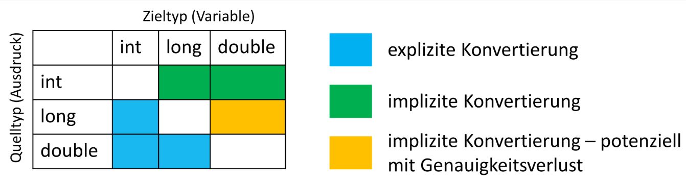
Back
Current
Note has been deleted
Field-by-field Comparison
| Field | Before | After |
|---|---|---|
| Occlusion | ||
| Image |
Note 1037: ETH::1. Semester::EProg
Deck: ETH::1. Semester::EProg
Note Type: Horvath Cloze
GUID:
deleted
Note Type: Horvath Cloze
GUID:
CRW*pWI6~N
Deleted Note
Front
Associativity of +, *, /, %: left-associative
Back
Associativity of +, *, /, %: left-associative
"X op Y op Z" is equivalent to "(X op Y) op Z"
Current
Note has been deleted
Field-by-field Comparison
| Field | Before | After |
|---|---|---|
| Text | ||
| Extra |
Note 1038: ETH::1. Semester::EProg
Deck: ETH::1. Semester::EProg
Note Type: Horvath Cloze
GUID:
deleted
Note Type: Horvath Cloze
GUID:
D,hN!b[~0a
Deleted Note
Front
Dog[] dogs = new Dog[5];
Animal[] animals = dogs; // Allowed! (upcasting)
animals[0] = new Cat(); // Compiles but ArrayStoreException at runtime!
Back
Dog[] dogs = new Dog[5];
Animal[] animals = dogs; // Allowed! (upcasting)
animals[0] = new Cat(); // Compiles but ArrayStoreException at runtime!
Current
Note has been deleted
Field-by-field Comparison
| Field | Before | After |
|---|---|---|
| Text |
Note 1039: ETH::1. Semester::EProg
Deck: ETH::1. Semester::EProg
Note Type: Horvath Cloze
GUID:
deleted
Note Type: Horvath Cloze
GUID:
D3~R~/O`**
Deleted Note
Front
instanceof tests whether an instance has a same dynamic type or if it implements an interface.Back
instanceof tests whether an instance has a same dynamic type or if it implements an interface.Current
Note has been deleted
Field-by-field Comparison
| Field | Before | After |
|---|---|---|
| Text |
Note 1040: ETH::1. Semester::EProg
Deck: ETH::1. Semester::EProg
Note Type: Horvath Cloze
GUID:
deleted
Note Type: Horvath Cloze
GUID:
DL*jz,QL[w
Deleted Note
Front
The weakest precondition for an empty program with postcondition false is false.
Back
The weakest precondition for an empty program with postcondition false is false.
As only false implies false.
Current
Note has been deleted
Field-by-field Comparison
| Field | Before | After |
|---|---|---|
| Text | ||
| Extra |
Note 1041: ETH::1. Semester::EProg
Deck: ETH::1. Semester::EProg
Note Type: Horvath Cloze
GUID:
deleted
Note Type: Horvath Cloze
GUID:
Dz$MyXFn=-
Deleted Note
Front
Casting like (double) binds stronger than +, -, /, %, *, etc...
Back
Casting like (double) binds stronger than +, -, /, %, *, etc...
As it's unary.
Current
Note has been deleted
Field-by-field Comparison
| Field | Before | After |
|---|---|---|
| Text | ||
| Extra |
Note 1042: ETH::1. Semester::EProg
Deck: ETH::1. Semester::EProg
Note Type: Horvath Cloze
GUID:
deleted
Note Type: Horvath Cloze
GUID:
D{XXurJu$`
Deleted Note
Front
short, int, float, double, long can be initialized using hexadecimal.
Back
short, int, float, double, long can be initialized using hexadecimal.
possibly also other types but definitely not boolean and char
Current
Note has been deleted
Field-by-field Comparison
| Field | Before | After |
|---|---|---|
| Text | ||
| Extra |
Note 1043: ETH::1. Semester::EProg
Deck: ETH::1. Semester::EProg
Note Type: Horvath Cloze
GUID:
deleted
Note Type: Horvath Cloze
GUID:
E(5s[CJXSQ
Deleted Note
Front
Casting to an interface only leads to a compile error for final classes.
Back
Casting to an interface only leads to a compile error for final classes.
Then no subclass could implement the interface.
Current
Note has been deleted
Field-by-field Comparison
| Field | Before | After |
|---|---|---|
| Text | ||
| Extra |
Note 1044: ETH::1. Semester::EProg
Deck: ETH::1. Semester::EProg
Note Type: Horvath Cloze
GUID:
deleted
Note Type: Horvath Cloze
GUID:
EYTdZt3/*5
Deleted Note
Front
Checked exceptions have to be announced or handled directly.
Back
Checked exceptions have to be announced or handled directly.
public void throwsStuff() throws CheckedException {
throws CheckedException(); // Allowed
}
public void throwsStuff() {
try {
throwsStuff();
} catch (Exception e) { }; // Allowed
}
Current
Note has been deleted
Field-by-field Comparison
| Field | Before | After |
|---|---|---|
| Text | ||
| Extra |
Note 1045: ETH::1. Semester::EProg
Deck: ETH::1. Semester::EProg
Note Type: Horvath Cloze
GUID:
deleted
Note Type: Horvath Cloze
GUID:
E_A@gwOm;?
Deleted Note
Front
The Arrays class has helper methods that make simple operations quicker:
- Arrays.equals(a, b) to compare arrays
- Arrays.copyOf(arr, l) that returns a new copied array of length l
- Sorting using Arrays.sort(arr)
- toString() and deepToString()
Back
The Arrays class has helper methods that make simple operations quicker:
- Arrays.equals(a, b) to compare arrays
- Arrays.copyOf(arr, l) that returns a new copied array of length l
- Sorting using Arrays.sort(arr)
- toString() and deepToString()
Arrays.deepToString() converts a nested/multidimensional array to a readable string representation, recursively handling inner arrays.
Current
Note has been deleted
Field-by-field Comparison
| Field | Before | After |
|---|---|---|
| Text | ||
| Extra |
Note 1046: ETH::1. Semester::EProg
Deck: ETH::1. Semester::EProg
Note Type: Horvath Classic
GUID:
deleted
Note Type: Horvath Classic
GUID:
E_rcts7/^g
Deleted Note
Front
while (i < n) {
result = result * k;
i = i + 1;
}
For the loop invariant, what bounds hold for i?
result = result * k;
i = i + 1;
}
For the loop invariant, what bounds hold for i?
Back
while (i < n) {
result = result * k;
i = i + 1;
}
For the loop invariant, what bounds hold for i?
result = result * k;
i = i + 1;
}
For the loop invariant, what bounds hold for i?
i <= n (the equality holds as we execute + 1 after the final execution)In general: x < n becomes x <= n and x <= n becomes x <= n + 1
Current
Note has been deleted
Field-by-field Comparison
| Field | Before | After |
|---|---|---|
| Front | ||
| Back |
Note 1047: ETH::1. Semester::EProg
Deck: ETH::1. Semester::EProg
Note Type: Horvath Cloze
GUID:
deleted
Note Type: Horvath Cloze
GUID:
El$[?h8w;k
Deleted Note
Front
Attribute access modifiers:
- default: package scoped, only available in same package.
- public: by everyone
- private: only accessible from within the object itself (not shared with other instances, unlike static)
- static: no initialisation needed, can be accessed through Math.PI
- final: prevents overwriting, like const
- protected: only by this class and subclasses
Back
Attribute access modifiers:
- default: package scoped, only available in same package.
- public: by everyone
- private: only accessible from within the object itself (not shared with other instances, unlike static)
- static: no initialisation needed, can be accessed through Math.PI
- final: prevents overwriting, like const
- protected: only by this class and subclasses
Current
Note has been deleted
Field-by-field Comparison
| Field | Before | After |
|---|---|---|
| Text |
Note 1048: ETH::1. Semester::EProg
Deck: ETH::1. Semester::EProg
Note Type: Horvath Cloze
GUID:
deleted
Note Type: Horvath Cloze
GUID:
E|{Z<-t*y@
Deleted Note
Front
Private attributes are accessible by all objects of this class.
Back
Private attributes are accessible by all objects of this class.
public class Rational {
private int x;
// Copy constructor
public Rational(Rational other) {
this.x = other.x; // We CAN access another objects private attributes
}
}
Current
Note has been deleted
Field-by-field Comparison
| Field | Before | After |
|---|---|---|
| Text | ||
| Extra |
Note 1049: ETH::1. Semester::EProg
Deck: ETH::1. Semester::EProg
Note Type: Horvath Cloze
GUID:
deleted
Note Type: Horvath Cloze
GUID:
F$o5lV^z=H
Deleted Note
Front
Note that a class can implement multiple interfaces.
If a method is defined in multiple of those interfaces, it of course has to be implemented only once.
Back
Note that a class can implement multiple interfaces.
If a method is defined in multiple of those interfaces, it of course has to be implemented only once.
Current
Note has been deleted
Field-by-field Comparison
| Field | Before | After |
|---|---|---|
| Text |
Note 1050: ETH::1. Semester::EProg
Deck: ETH::1. Semester::EProg
Note Type: Horvath Cloze
GUID:
deleted
Note Type: Horvath Cloze
GUID:
F405hHI@j2
Deleted Note
Front
A Java name is called an identifier.
Back
A Java name is called an identifier.
Current
Note has been deleted
Field-by-field Comparison
| Field | Before | After |
|---|---|---|
| Text |
Note 1051: ETH::1. Semester::EProg
Deck: ETH::1. Semester::EProg
Note Type: Horvath Cloze
GUID:
deleted
Note Type: Horvath Cloze
GUID:
FXUR__;!h6
Deleted Note
Front
When a function is called in dynamic dispatch, the attributes of the type in which the actual function is executed will be used.
Back
When a function is called in dynamic dispatch, the attributes of the type in which the actual function is executed will be used.
class T {
int data = 50;
public void s2() {
System.out.println("T " + data);
}
}
class S extends T {
int data = 100;
public void s2() { System.out.println(this.data);
}
}
class R extends S {
int data = 200;
}
T r = new R();
r.s2(); // Prints "100"
Current
Note has been deleted
Field-by-field Comparison
| Field | Before | After |
|---|---|---|
| Text | ||
| Extra |
Note 1052: ETH::1. Semester::EProg
Deck: ETH::1. Semester::EProg
Note Type: Horvath Cloze
GUID:
deleted
Note Type: Horvath Cloze
GUID:
FwBjd_dmb+
Deleted Note
Front
Constructors are not inherited by subclasses.
Back
Constructors are not inherited by subclasses.
Current
Note has been deleted
Field-by-field Comparison
| Field | Before | After |
|---|---|---|
| Text |
Note 1053: ETH::1. Semester::EProg
Deck: ETH::1. Semester::EProg
Note Type: Horvath Classic
GUID:
deleted
Note Type: Horvath Classic
GUID:
G#$#7KW!b}
Deleted Note
Front
instanceof can result in a Compile-/Runtime-/No error?
Back
instanceof can result in a Compile-/Runtime-/No error?
instanceof never throws an exception, just compile errors.Current
Note has been deleted
Field-by-field Comparison
| Field | Before | After |
|---|---|---|
| Front | ||
| Back |
Note 1054: ETH::1. Semester::EProg
Deck: ETH::1. Semester::EProg
Note Type: Horvath Cloze
GUID:
deleted
Note Type: Horvath Cloze
GUID:
G&=W~#L|H<
Deleted Note
Front
There are checked and unchecked exceptions.
Back
There are checked and unchecked exceptions.
Current
Note has been deleted
Field-by-field Comparison
| Field | Before | After |
|---|---|---|
| Text |
Note 1055: ETH::1. Semester::EProg
Deck: ETH::1. Semester::EProg
Note Type: Horvath Cloze
GUID:
deleted
Note Type: Horvath Cloze
GUID:
G]t&7SvtKp
Deleted Note
Front
In a dynamic dispatch, the "this"-keyword still refers to the dynamic type, thus even if the method is in a superclass, it will always try to use the "most overriden" method.
Back
In a dynamic dispatch, the "this"-keyword still refers to the dynamic type, thus even if the method is in a superclass, it will always try to use the "most overriden" method.
Current
Note has been deleted
Field-by-field Comparison
| Field | Before | After |
|---|---|---|
| Text |
Note 1056: ETH::1. Semester::EProg
Deck: ETH::1. Semester::EProg
Note Type: Horvath Cloze
GUID:
deleted
Note Type: Horvath Cloze
GUID:
H%0Tkaz:@S
Deleted Note
Front
Interfaces don't define behaviour, only method signatures.
Back
Interfaces don't define behaviour, only method signatures.
Current
Note has been deleted
Field-by-field Comparison
| Field | Before | After |
|---|---|---|
| Text |
Note 1057: ETH::1. Semester::EProg
Deck: ETH::1. Semester::EProg
Note Type: Horvath Cloze
GUID:
deleted
Note Type: Horvath Cloze
GUID:
H=AHLUgZxW
Deleted Note
Front
Java double can be initialised with
- 32.300 "." seperated numbers
- 1e-2 exponentials
Back
Java double can be initialised with
- 32.300 "." seperated numbers
- 1e-2 exponentials
Current
Note has been deleted
Field-by-field Comparison
| Field | Before | After |
|---|---|---|
| Text |
Note 1058: ETH::1. Semester::EProg
Deck: ETH::1. Semester::EProg
Note Type: Horvath Cloze
GUID:
deleted
Note Type: Horvath Cloze
GUID:
HI3~1]W{fH
Deleted Note
Front
if we have final Cat c = new Cat() the reference is immutable but the attributes of the class are not.
Back
if we have final Cat c = new Cat() the reference is immutable but the attributes of the class are not.
Current
Note has been deleted
Field-by-field Comparison
| Field | Before | After |
|---|---|---|
| Text |
Note 1059: ETH::1. Semester::EProg
Deck: ETH::1. Semester::EProg
Note Type: Horvath Classic
GUID:
deleted
Note Type: Horvath Classic
GUID:
HNxps|u:&w
Deleted Note
Front
How are enums initialized?
Back
How are enums initialized?
public enum Status {
SUBMITTED,
PAID,
...
}
SUBMITTED,
PAID,
...
}
Current
Note has been deleted
Field-by-field Comparison
| Field | Before | After |
|---|---|---|
| Front | ||
| Back |
Note 1060: ETH::1. Semester::EProg
Deck: ETH::1. Semester::EProg
Note Type: Horvath Cloze
GUID:
deleted
Note Type: Horvath Cloze
GUID:
HY!(CO](X8
Deleted Note
Front
Private methods are not inherited from the superclass and cannot be called (same as for private attributes).
Back
Private methods are not inherited from the superclass and cannot be called (same as for private attributes).
Current
Note has been deleted
Field-by-field Comparison
| Field | Before | After |
|---|---|---|
| Text |
Note 1061: ETH::1. Semester::EProg
Deck: ETH::1. Semester::EProg
Note Type: Horvath Cloze
GUID:
deleted
Note Type: Horvath Cloze
GUID:
Hf&j3}sSGT
Deleted Note
Front
== and <, etc... have higher precedence than boolean comparison operators like &&, ||
Back
== and <, etc... have higher precedence than boolean comparison operators like &&, ||
Current
Note has been deleted
Field-by-field Comparison
| Field | Before | After |
|---|---|---|
| Text |
Note 1062: ETH::1. Semester::EProg
Deck: ETH::1. Semester::EProg
Note Type: Horvath Cloze
GUID:
deleted
Note Type: Horvath Cloze
GUID:
Hz_:Sp*X(y
Deleted Note
Front
class A {
public int x = 5;
}
class B extends A {
public int y = 6;
public int test() { return 0; } public B(int i) {
super();
}}
A a1 = new B(1);
a1.y; // leads to a compile error, as A doesn't have x
a1.test(); // leads to a compile error, as A doesn't have test()Back
class A {
public int x = 5;
}
class B extends A {
public int y = 6;
public int test() { return 0; } public B(int i) {
super();
}}
A a1 = new B(1);
a1.y; // leads to a compile error, as A doesn't have x
a1.test(); // leads to a compile error, as A doesn't have test()Current
Note has been deleted
Field-by-field Comparison
| Field | Before | After |
|---|---|---|
| Text |
Note 1063: ETH::1. Semester::EProg
Deck: ETH::1. Semester::EProg
Note Type: Horvath Classic
GUID:
deleted
Note Type: Horvath Classic
GUID:
I0s;#,Wh%?
Deleted Note
Front
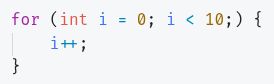
Compile/Runtime/No Error
Back
Compile/Runtime/No Error
No error, valid for loop.
Current
Note has been deleted
Field-by-field Comparison
| Field | Before | After |
|---|---|---|
| Front | ||
| Back |
Note 1064: ETH::1. Semester::EProg
Deck: ETH::1. Semester::EProg
Note Type: Horvath Classic
GUID:
deleted
Note Type: Horvath Classic
GUID:
IKMb!{98`
Deleted Note
Front
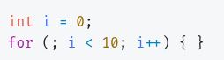
Compile/Runtime/No Error?
Back
Compile/Runtime/No Error?
Valid for-loop.
Current
Note has been deleted
Field-by-field Comparison
| Field | Before | After |
|---|---|---|
| Front | ||
| Back |
Note 1065: ETH::1. Semester::EProg
Deck: ETH::1. Semester::EProg
Note Type: Horvath Cloze
GUID:
deleted
Note Type: Horvath Cloze
GUID:
IQ4$mZs7/D
Deleted Note
Front
The 8 primitve types of Java are:
- byte
- char
- short
- int
- long
- float
- double
- boolean
Back
The 8 primitve types of Java are:
- byte
- char
- short
- int
- long
- float
- double
- boolean
Current
Note has been deleted
Field-by-field Comparison
| Field | Before | After |
|---|---|---|
| Text |
Note 1066: ETH::1. Semester::EProg
Deck: ETH::1. Semester::EProg
Note Type: Image Occlusion-73a2c
GUID:
deleted
Note Type: Image Occlusion-73a2c
GUID:
IdA(dVgMPN
Deleted Note
Front
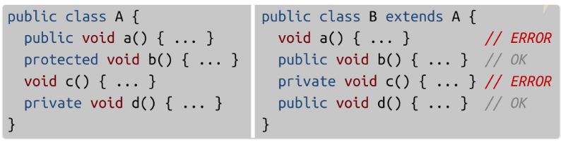
Back
Current
Note has been deleted
Field-by-field Comparison
| Field | Before | After |
|---|---|---|
| Occlusion | ||
| Image |
Note 1067: ETH::1. Semester::EProg
Deck: ETH::1. Semester::EProg
Note Type: Horvath Cloze
GUID:
deleted
Note Type: Horvath Cloze
GUID:
Ih(!XjbZQJ
Deleted Note
Front
Die Sprache einer EBNF-Beschreibung ist die Menge aller legalen Zeichenfolgen.
Back
Die Sprache einer EBNF-Beschreibung ist die Menge aller legalen Zeichenfolgen.
Current
Note has been deleted
Field-by-field Comparison
| Field | Before | After |
|---|---|---|
| Text |
Note 1068: ETH::1. Semester::EProg
Deck: ETH::1. Semester::EProg
Note Type: Horvath Classic
GUID:
deleted
Note Type: Horvath Classic
GUID:
J#D+xVYd4z
Deleted Note
Front
(double) 3 / 2 evaluates to?
(double) (3 / 2) evaluates to?
(double) (3 / 2) evaluates to?
Back
(double) 3 / 2 evaluates to?
(double) (3 / 2) evaluates to?
(double) (3 / 2) evaluates to?
1.5
1.0
As casting has stronger precedence.
1.0
As casting has stronger precedence.
Current
Note has been deleted
Field-by-field Comparison
| Field | Before | After |
|---|---|---|
| Front | ||
| Back |
Note 1069: ETH::1. Semester::EProg
Deck: ETH::1. Semester::EProg
Note Type: Horvath Classic
GUID:
deleted
Note Type: Horvath Classic
GUID:
J)-A!rQ/Od
Deleted Note
Front
int[][] b = new int[3][0]int[] c = new int[3] b[0] = c
Is this fine?
Back
int[][] b = new int[3][0]int[] c = new int[3] b[0] = c
Is this fine?
Yes, it works fine as we just set the pointer of b[0] to c. Java does not typecheck array dimensions.
Current
Note has been deleted
Field-by-field Comparison
| Field | Before | After |
|---|---|---|
| Front | ||
| Back |
Note 1070: ETH::1. Semester::EProg
Deck: ETH::1. Semester::EProg
Note Type: Horvath Classic
GUID:
deleted
Note Type: Horvath Classic
GUID:
JX37U6@Pja
Deleted Note
Front
++x does what?
Back
++x does what?
Pre-Increment: increments x then returns it's value
Current
Note has been deleted
Field-by-field Comparison
| Field | Before | After |
|---|---|---|
| Front | ||
| Back |
Note 1071: ETH::1. Semester::EProg
Deck: ETH::1. Semester::EProg
Note Type: Horvath Cloze
GUID:
deleted
Note Type: Horvath Cloze
GUID:
J`K7cc2By_
Deleted Note
Front
List<Dog> dogs = new ArrayList<>();
List<Animal> animals = (List<Animal>) dogs; // Unchecked cast warningBack
List<Dog> dogs = new ArrayList<>();
List<Animal> animals = (List<Animal>) dogs; // Unchecked cast warningNo Error because of type erasure here.
Current
Note has been deleted
Field-by-field Comparison
| Field | Before | After |
|---|---|---|
| Text | ||
| Extra |
Note 1072: ETH::1. Semester::EProg
Deck: ETH::1. Semester::EProg
Note Type: Horvath Classic
GUID:
deleted
Note Type: Horvath Classic
GUID:
KZF4,Q[f&D
Deleted Note
Front
We can catch exceptions using:
Back
We can catch exceptions using:
try { } catch (ExceptionName e) { };Current
Note has been deleted
Field-by-field Comparison
| Field | Before | After |
|---|---|---|
| Front | ||
| Back |
Note 1073: ETH::1. Semester::EProg
Deck: ETH::1. Semester::EProg
Note Type: Horvath Cloze
GUID:
deleted
Note Type: Horvath Cloze
GUID:
K]ZyP_vxG;
Deleted Note
Front
Inside a class (except static functions) we have access to special variable this and super.
Back
Inside a class (except static functions) we have access to special variable this and super.
Current
Note has been deleted
Field-by-field Comparison
| Field | Before | After |
|---|---|---|
| Text |
Note 1074: ETH::1. Semester::EProg
Deck: ETH::1. Semester::EProg
Note Type: Horvath Cloze
GUID:
deleted
Note Type: Horvath Cloze
GUID:
KhTp)`Z~|8
Deleted Note
Front
Strings are immutable.
Back
Strings are immutable.
Current
Note has been deleted
Field-by-field Comparison
| Field | Before | After |
|---|---|---|
| Text |
Note 1075: ETH::1. Semester::EProg
Deck: ETH::1. Semester::EProg
Note Type: Horvath Cloze
GUID:
deleted
Note Type: Horvath Cloze
GUID:
KnKuMTM<[8
Deleted Note
Front
A protected attribute can also be accessed by subclasses.
Back
A protected attribute can also be accessed by subclasses.
Current
Note has been deleted
Field-by-field Comparison
| Field | Before | After |
|---|---|---|
| Text |
Note 1076: ETH::1. Semester::EProg
Deck: ETH::1. Semester::EProg
Note Type: Horvath Classic
GUID:
deleted
Note Type: Horvath Classic
GUID:
LHfofYY0cF
Deleted Note
Front
Can we use ++ and -- on floats and doubles?
Back
Can we use ++ and -- on floats and doubles?
Yes, that is allowed and increments by 1.0.
Current
Note has been deleted
Field-by-field Comparison
| Field | Before | After |
|---|---|---|
| Front | ||
| Back |
Note 1077: ETH::1. Semester::EProg
Deck: ETH::1. Semester::EProg
Note Type: Horvath Cloze
GUID:
deleted
Note Type: Horvath Cloze
GUID:
LdyT3WH.QQ
Deleted Note
Front
Casting to an interface (if not implemented) leads to a runtime error.
Back
Casting to an interface (if not implemented) leads to a runtime error.
The compiler always assumes a subtype could implement the class.
Current
Note has been deleted
Field-by-field Comparison
| Field | Before | After |
|---|---|---|
| Text | ||
| Extra |
Note 1078: ETH::1. Semester::EProg
Deck: ETH::1. Semester::EProg
Note Type: Horvath Cloze
GUID:
deleted
Note Type: Horvath Cloze
GUID:
MQ0U{K
Deleted Note
Front
We can access the parent's attribute of a subclass by casting to the static type of the parent.
Back
We can access the parent's attribute of a subclass by casting to the static type of the parent.
Current
Note has been deleted
Field-by-field Comparison
| Field | Before | After |
|---|---|---|
| Text |
Note 1079: ETH::1. Semester::EProg
Deck: ETH::1. Semester::EProg
Note Type: Horvath Classic
GUID:
deleted
Note Type: Horvath Classic
GUID:
MlNjJv:07k
Deleted Note
Front
String s1 = "test";
String s2 = "test";
s1 == s2 returns?
String s2 = "test";
s1 == s2 returns?
Back
String s1 = "test";
String s2 = "test";
s1 == s2 returns?
String s2 = "test";
s1 == s2 returns?
Usually false, as we compare references. To compare strings we should use .equals().
Current
Note has been deleted
Field-by-field Comparison
| Field | Before | After |
|---|---|---|
| Front | ||
| Back |
Note 1080: ETH::1. Semester::EProg
Deck: ETH::1. Semester::EProg
Note Type: Horvath Cloze
GUID:
deleted
Note Type: Horvath Cloze
GUID:
MpWDjk%Tfz
Deleted Note
Front
Instance of returns true if:
- Implements the interface
- Is of the same dynamic type
- Is a subtype of the dynamic type
Back
Instance of returns true if:
- Implements the interface
- Is of the same dynamic type
- Is a subtype of the dynamic type
Current
Note has been deleted
Field-by-field Comparison
| Field | Before | After |
|---|---|---|
| Text |
Note 1081: ETH::1. Semester::EProg
Deck: ETH::1. Semester::EProg
Note Type: Horvath Cloze
GUID:
deleted
Note Type: Horvath Cloze
GUID:
MqC&7Qly55
Deleted Note
Front
class A {
public int x = 5;
public void fct1() {
System.out.println(this.x);
}
}
class B extends A {
public B() {
super.x = 10;
}
public B(int a) {
super.x = a;
}
}
A a1 = new B(1);
A a2 = new B(12); // As these are different instances, their attributes are separate
B b1 = new B(1);
B b2 = new B(12);
a1.fct1(); // 1 -> Even though static type is A
a2.fct1(); // 12 -> Different output as a2's instance of A has 12
b1.fct1(); // 1 -> same here, even though it dynamic dispatches
b2.fct1(); // 12
Back
class A {
public int x = 5;
public void fct1() {
System.out.println(this.x);
}
}
class B extends A {
public B() {
super.x = 10;
}
public B(int a) {
super.x = a;
}
}
A a1 = new B(1);
A a2 = new B(12); // As these are different instances, their attributes are separate
B b1 = new B(1);
B b2 = new B(12);
a1.fct1(); // 1 -> Even though static type is A
a2.fct1(); // 12 -> Different output as a2's instance of A has 12
b1.fct1(); // 1 -> same here, even though it dynamic dispatches
b2.fct1(); // 12
Current
Note has been deleted
Field-by-field Comparison
| Field | Before | After |
|---|---|---|
| Text |
Note 1082: ETH::1. Semester::EProg
Deck: ETH::1. Semester::EProg
Note Type: Horvath Classic
GUID:
deleted
Note Type: Horvath Classic
GUID:
N,~U9>@HR@
Deleted Note
Front
How do we implement a subtype in Java?
Back
How do we implement a subtype in Java?
public class Lorenz extends Students {
@Override
public void someMethod() {
...
super.someMethod(); // Can call super's implementation of this
}
}
Current
Note has been deleted
Field-by-field Comparison
| Field | Before | After |
|---|---|---|
| Front | ||
| Back |
Note 1083: ETH::1. Semester::EProg
Deck: ETH::1. Semester::EProg
Note Type: Horvath Classic
GUID:
deleted
Note Type: Horvath Classic
GUID:
N/)4j!wS3C
Deleted Note
Front
Which of the following is (or are) NOT a Java keyword?
- volatile
- mod
- strictfp
- loop
- transient
- do
- use
- volatile
- mod
- strictfp
- loop
- transient
- do
- use
Back
Which of the following is (or are) NOT a Java keyword?
- volatile
- mod
- strictfp
- loop
- transient
- do
- use
- volatile
- mod
- strictfp
- loop
- transient
- do
- use
loop, use and mod
Current
Note has been deleted
Field-by-field Comparison
| Field | Before | After |
|---|---|---|
| Front | ||
| Back |
Note 1084: ETH::1. Semester::EProg
Deck: ETH::1. Semester::EProg
Note Type: Horvath Cloze
GUID:
deleted
Note Type: Horvath Cloze
GUID:
Nz^YQRPVQ2
Deleted Note
Front
Properties of classes declared as public int x; are set to their default values (0, null, false, etc...).
Back
Properties of classes declared as public int x; are set to their default values (0, null, false, etc...).
Current
Note has been deleted
Field-by-field Comparison
| Field | Before | After |
|---|---|---|
| Text |
Note 1085: ETH::1. Semester::EProg
Deck: ETH::1. Semester::EProg
Note Type: Horvath Cloze
GUID:
deleted
Note Type: Horvath Cloze
GUID:
O:PCKgyN)+
Deleted Note
Front
Java uses dynamic dispatch for function calls, we therefore get the method of the dynamic type.
Back
Java uses dynamic dispatch for function calls, we therefore get the method of the dynamic type.
Current
Note has been deleted
Field-by-field Comparison
| Field | Before | After |
|---|---|---|
| Text |
Note 1086: ETH::1. Semester::EProg
Deck: ETH::1. Semester::EProg
Note Type: Horvath Cloze
GUID:
deleted
Note Type: Horvath Cloze
GUID:
O@-k%ZU440
Deleted Note
Front
Accessing the parent's parent's variables in Java is not allowed.
Back
Accessing the parent's parent's variables in Java is not allowed.
Current
Note has been deleted
Field-by-field Comparison
| Field | Before | After |
|---|---|---|
| Text |
Note 1087: ETH::1. Semester::EProg
Deck: ETH::1. Semester::EProg
Note Type: Horvath Cloze
GUID:
deleted
Note Type: Horvath Cloze
GUID:
OGFJDr03D}
Deleted Note
Front
super.super.xxx, or x.super.xxx are not allowed an give a compile error.Back
super.super.xxx, or x.super.xxx are not allowed an give a compile error.Current
Note has been deleted
Field-by-field Comparison
| Field | Before | After |
|---|---|---|
| Text |
Note 1088: ETH::1. Semester::EProg
Deck: ETH::1. Semester::EProg
Note Type: Horvath Cloze
GUID:
deleted
Note Type: Horvath Cloze
GUID:
OGFye&*Y@Y
Deleted Note
Front
The compiler uses the static type to get attributes.
Back
The compiler uses the static type to get attributes.
Current
Note has been deleted
Field-by-field Comparison
| Field | Before | After |
|---|---|---|
| Text |
Note 1089: ETH::1. Semester::EProg
Deck: ETH::1. Semester::EProg
Note Type: Horvath Cloze
GUID:
deleted
Note Type: Horvath Cloze
GUID:
OJ16/M<6a6
Deleted Note
Front
An option in EBNF can be written as [ E ] or E | \(\epsilon\).
Back
An option in EBNF can be written as [ E ] or E | \(\epsilon\).
Current
Note has been deleted
Field-by-field Comparison
| Field | Before | After |
|---|---|---|
| Text |
Note 1090: ETH::1. Semester::EProg
Deck: ETH::1. Semester::EProg
Note Type: Horvath Classic
GUID:
deleted
Note Type: Horvath Classic
GUID:
P6>K30cX4E
Deleted Note
Front
How could someone modify a private variable (aliasing)?
Back
How could someone modify a private variable (aliasing)?
public class AliasingProblem {
private Point center; // Problematic - exposes internal reference
public Point getCenter() {
return center; // Returns alias to internal object
}
}
main() {
Point center = new AliasingProblem().getCenter();
center.setX(2); // Changes private attribute!!
}
If we get a reference to a private object, we can indeed change it's values!
Current
Note has been deleted
Field-by-field Comparison
| Field | Before | After |
|---|---|---|
| Front | ||
| Back |
Note 1091: ETH::1. Semester::EProg
Deck: ETH::1. Semester::EProg
Note Type: Horvath Classic
GUID:
deleted
Note Type: Horvath Classic
GUID:
PReOU!^g*#
Deleted Note
Front
do {
// body
} while (test);
statement;
Does what?
// body
} while (test);
statement;
Does what?
Back
do {
// body
} while (test);
statement;
Does what?
// body
} while (test);
statement;
Does what?
First the body is executed at least a single time, then the condition evaluated.
Current
Note has been deleted
Field-by-field Comparison
| Field | Before | After |
|---|---|---|
| Front | ||
| Back |
Note 1092: ETH::1. Semester::EProg
Deck: ETH::1. Semester::EProg
Note Type: Horvath Cloze
GUID:
deleted
Note Type: Horvath Cloze
GUID:
Pi]A?I0a.)
Deleted Note
Front
In a subclass, we can access the parent's methods and attributes using super.
Back
In a subclass, we can access the parent's methods and attributes using super.
You cannot use
super.super.xxx, nor x.super.xxx to access super methods or attributes. This gives a compile error.Current
Note has been deleted
Field-by-field Comparison
| Field | Before | After |
|---|---|---|
| Text | ||
| Extra |
Note 1093: ETH::1. Semester::EProg
Deck: ETH::1. Semester::EProg
Note Type: Horvath Classic
GUID:
deleted
Note Type: Horvath Classic
GUID:
Q=BFp=(vY3
Deleted Note
Front
The ternary operator has the following syntax:
Back
The ternary operator has the following syntax:
test ? valueTrue : valueFalse
Current
Note has been deleted
Field-by-field Comparison
| Field | Before | After |
|---|---|---|
| Front | ||
| Back |
Note 1094: ETH::1. Semester::EProg
Deck: ETH::1. Semester::EProg
Note Type: Horvath Cloze
GUID:
deleted
Note Type: Horvath Cloze
GUID:
QEMy5L&
Deleted Note
Front
class A { int x; }
class B extends A { boolean x; }
A a = new A();
a.x = 6; // OK
a.x = true; // Compile error, type mismatch
A a = new B();
a.x = 6; // OK
a.x = true; // Compile error, type mismatch because static type is used
B b = new B();
b.x = 6; // Type Error
b.x = true; // OK!
Back
class A { int x; }
class B extends A { boolean x; }
A a = new A();
a.x = 6; // OK
a.x = true; // Compile error, type mismatch
A a = new B();
a.x = 6; // OK
a.x = true; // Compile error, type mismatch because static type is used
B b = new B();
b.x = 6; // Type Error
b.x = true; // OK!
Current
Note has been deleted
Field-by-field Comparison
| Field | Before | After |
|---|---|---|
| Text |
Note 1095: ETH::1. Semester::EProg
Deck: ETH::1. Semester::EProg
Note Type: Horvath Cloze
GUID:
deleted
Note Type: Horvath Cloze
GUID:
bxDOHVL#p]
Deleted Note
Front
The cases where instanceof causes a compile error:
- Primitives - instanceof only works with reference types
- Generics - type erasure means List<String> becomes just List at runtime, so the check is impossible
t instanceof List<String> - Unrelated types:
Animal -> DogandAnimal -> Cat.
Check foranimal instanceof Dog/Catallowed, butdog = new Dog(); dog instanceof Catthrows compile error. - Final class - if a class is final and doesn't implement an interface, no subclass could ever implement it, so the check is provably always false.
Back
The cases where instanceof causes a compile error:
- Primitives - instanceof only works with reference types
- Generics - type erasure means List<String> becomes just List at runtime, so the check is impossible
t instanceof List<String> - Unrelated types:
Animal -> DogandAnimal -> Cat.
Check foranimal instanceof Dog/Catallowed, butdog = new Dog(); dog instanceof Catthrows compile error. - Final class - if a class is final and doesn't implement an interface, no subclass could ever implement it, so the check is provably always false.
However:
Animal a = getanimal() could get a Dog which might implement List thus a instanceof List is not a compile error.Current
Note has been deleted
Field-by-field Comparison
| Field | Before | After |
|---|---|---|
| Text | ||
| Extra |
Note 1096: ETH::1. Semester::EProg
Deck: ETH::1. Semester::EProg
Note Type: Horvath Cloze
GUID:
deleted
Note Type: Horvath Cloze
GUID:
c>xF]nJjL8
Deleted Note
Front
Animal cat = null; (Cat) cat; Leads to a no error, this is always allowed.
Back
Animal cat = null; (Cat) cat; Leads to a no error, this is always allowed.
Current
Note has been deleted
Field-by-field Comparison
| Field | Before | After |
|---|---|---|
| Text |
Note 1097: ETH::1. Semester::EProg
Deck: ETH::1. Semester::EProg
Note Type: Horvath Classic
GUID:
deleted
Note Type: Horvath Classic
GUID:
cT=vzGuBpg
Deleted Note
Front
5 == 5 || String.yourStupidAss() evaluates to ???
Back
5 == 5 || String.yourStupidAss() evaluates to ???
Compile Error, even if it shortcircuits.
Current
Note has been deleted
Field-by-field Comparison
| Field | Before | After |
|---|---|---|
| Front | ||
| Back |
Note 1098: ETH::1. Semester::EProg
Deck: ETH::1. Semester::EProg
Note Type: Horvath Cloze
GUID:
deleted
Note Type: Horvath Cloze
GUID:
dBkAd*&?D6
Deleted Note
Front
The dynamic type is always a subtype of the static type.
Back
The dynamic type is always a subtype of the static type.
Current
Note has been deleted
Field-by-field Comparison
| Field | Before | After |
|---|---|---|
| Text |
Note 1099: ETH::1. Semester::EProg
Deck: ETH::1. Semester::EProg
Note Type: Horvath Classic
GUID:
deleted
Note Type: Horvath Classic
GUID:
dE4W+,!/H<
Deleted Note
Front
5++ evaluates to ???
Back
5++ evaluates to ???
compile error, 5 is not a variable.
Current
Note has been deleted
Field-by-field Comparison
| Field | Before | After |
|---|---|---|
| Front | ||
| Back |
Note 1100: ETH::1. Semester::EProg
Deck: ETH::1. Semester::EProg
Note Type: Horvath Cloze
GUID:
deleted
Note Type: Horvath Cloze
GUID:
dW?TP?RI{A
Deleted Note
Front
The dynamic type of a variable can be changed by reassigning the reference to another instance.
Back
The dynamic type of a variable can be changed by reassigning the reference to another instance.
Current
Note has been deleted
Field-by-field Comparison
| Field | Before | After |
|---|---|---|
| Text |
Note 1101: ETH::1. Semester::EProg
Deck: ETH::1. Semester::EProg
Note Type: Horvath Cloze
GUID:
deleted
Note Type: Horvath Cloze
GUID:
e>j3maYE+y
Deleted Note
Front
Every primitive variable must be both declared and initialized before being used.
Back
Every primitive variable must be both declared and initialized before being used.
This is only true for local variables! Instance variables can be left uninitialised.
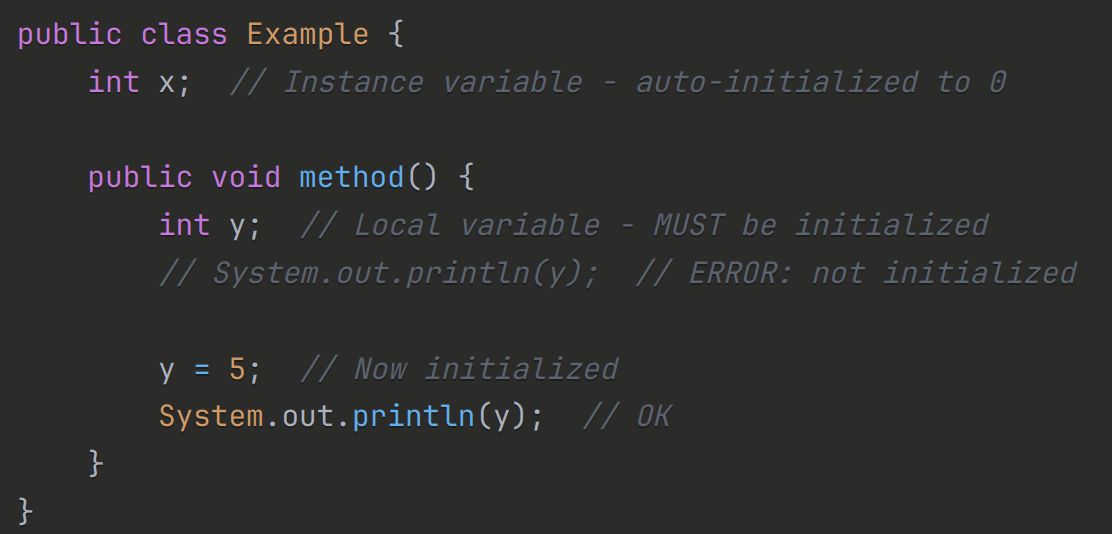
Current
Note has been deleted
Field-by-field Comparison
| Field | Before | After |
|---|---|---|
| Text | ||
| Extra |
Note 1102: ETH::1. Semester::EProg
Deck: ETH::1. Semester::EProg
Note Type: Horvath Classic
GUID:
deleted
Note Type: Horvath Classic
GUID:
eEx@10sK[?
Deleted Note
Front
What is the difference between i++ and ++i in Java?
Back
What is the difference between i++ and ++i in Java?
i++ returns the current value of i and then increments i by 1
++i first increments value of i by 1 and then returns the value
++i first increments value of i by 1 and then returns the value
Current
Note has been deleted
Field-by-field Comparison
| Field | Before | After |
|---|---|---|
| Front | ||
| Back |
Note 1103: ETH::1. Semester::EProg
Deck: ETH::1. Semester::EProg
Note Type: Horvath Cloze
GUID:
deleted
Note Type: Horvath Cloze
GUID:
f2vR,E9IiI
Deleted Note
Front
Unary operators bind stronger than binary ones.
Back
Unary operators bind stronger than binary ones.
Current
Note has been deleted
Field-by-field Comparison
| Field | Before | After |
|---|---|---|
| Text |
Note 1104: ETH::1. Semester::EProg
Deck: ETH::1. Semester::EProg
Note Type: Horvath Cloze
GUID:
deleted
Note Type: Horvath Cloze
GUID:
f3eqMn1(f/
Deleted Note
Front
Trying to access a method or attribute on a class with a different dynamic than static type leads to a compile error if the static type doesn't define that attribute or method.
Back
Trying to access a method or attribute on a class with a different dynamic than static type leads to a compile error if the static type doesn't define that attribute or method.
Current
Note has been deleted
Field-by-field Comparison
| Field | Before | After |
|---|---|---|
| Text |
Note 1105: ETH::1. Semester::EProg
Deck: ETH::1. Semester::EProg
Note Type: Horvath Classic
GUID:
deleted
Note Type: Horvath Classic
GUID:
fJL&tF*QW&
Deleted Note
Front
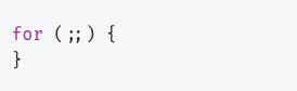
Compile/Runtime/no Error
Back
Compile/Runtime/no Error
No error, valid for loop
Current
Note has been deleted
Field-by-field Comparison
| Field | Before | After |
|---|---|---|
| Front | ||
| Back |
Note 1106: ETH::1. Semester::EProg
Deck: ETH::1. Semester::EProg
Note Type: Horvath Cloze
GUID:
deleted
Note Type: Horvath Cloze
GUID:
fx//I5}Q?7
Deleted Note
Front
Runtime Errors for Casting:
(Husky) dog;Casting further down than dynamic type(Cat) dog;Casting into sibling type
Back
Runtime Errors for Casting:
(Husky) dog;Casting further down than dynamic type(Cat) dog;Casting into sibling type
Current
Note has been deleted
Field-by-field Comparison
| Field | Before | After |
|---|---|---|
| Text |
Note 1107: ETH::1. Semester::EProg
Deck: ETH::1. Semester::EProg
Note Type: Horvath Cloze
GUID:
deleted
Note Type: Horvath Cloze
GUID:
g%YZ@`35DU
Deleted Note
Front
In a subclass, we can only make methods more visible .
Back
In a subclass, we can only make methods more visible .
- protected -> public is okay
- private -> public okay
public to default or default to private are not possible.
Current
Note has been deleted
Field-by-field Comparison
| Field | Before | After |
|---|---|---|
| Text | ||
| Extra |
Note 1108: ETH::1. Semester::EProg
Deck: ETH::1. Semester::EProg
Note Type: Horvath Cloze
GUID:
deleted
Note Type: Horvath Cloze
GUID:
g
Deleted Note
Front
A selection from several elements is written as A | B | C.
Back
A selection from several elements is written as A | B | C.
Current
Note has been deleted
Field-by-field Comparison
| Field | Before | After |
|---|---|---|
| Text |
Note 1109: ETH::1. Semester::EProg
Deck: ETH::1. Semester::EProg
Note Type: Horvath Cloze
GUID:
deleted
Note Type: Horvath Cloze
GUID:
gAXH/(0;9S
Deleted Note
Front
Class Cat should be declared in the file Cat.java.
Back
Class Cat should be declared in the file Cat.java.
But it does not HAVE TO be declared there, as long as it is not declared as public.
Current
Note has been deleted
Field-by-field Comparison
| Field | Before | After |
|---|---|---|
| Text | ||
| Extra |
Note 1110: ETH::1. Semester::EProg
Deck: ETH::1. Semester::EProg
Note Type: Horvath Classic
GUID:
deleted
Note Type: Horvath Classic
GUID:
gK8R,r`Ne1
Deleted Note
Front
How is a % b defined in Java?
Back
How is a % b defined in Java?
(a / b) * b + (a % b) = a (with a / b being division with rest)
In general, if the a is negative, the result is negative.
Current
Note has been deleted
Field-by-field Comparison
| Field | Before | After |
|---|---|---|
| Front | ||
| Back |
Note 1111: ETH::1. Semester::EProg
Deck: ETH::1. Semester::EProg
Note Type: Horvath Cloze
GUID:
deleted
Note Type: Horvath Cloze
GUID:
g_DbKK.&&1
Deleted Note
Front
Downcasting like (B) A will lead to runtime errors if A is not of type or subtype B.
Back
Downcasting like (B) A will lead to runtime errors if A is not of type or subtype B.
Current
Note has been deleted
Field-by-field Comparison
| Field | Before | After |
|---|---|---|
| Text |
Note 1112: ETH::1. Semester::EProg
Deck: ETH::1. Semester::EProg
Note Type: Horvath Cloze
GUID:
deleted
Note Type: Horvath Cloze
GUID:
gc|oK]2yr^
Deleted Note
Front
We cannot override attributes inside a subclass, they are shadowed.
Back
We cannot override attributes inside a subclass, they are shadowed.
class Animal {
String name = "Animal";
String getName() {
return "Animal";
}
}
class Dog extends Animal {
String name = "Dog"; // Shadows Animal.name (doesn't override it)
@Override String getName() { return Dog"; } // Overrides Animal.getName()
}
Animal a = new Dog();
System.out.println(a.name); // "Animal" — field access uses static type
System.out.println(a.getName()); // "Dog" — method call uses dynamic type
Current
Note has been deleted
Field-by-field Comparison
| Field | Before | After |
|---|---|---|
| Text | ||
| Extra |
Note 1113: ETH::1. Semester::EProg
Deck: ETH::1. Semester::EProg
Note Type: Image Occlusion-73a2c
GUID:
deleted
Note Type: Image Occlusion-73a2c
GUID:
gef_5DD5?n
Deleted Note
Front
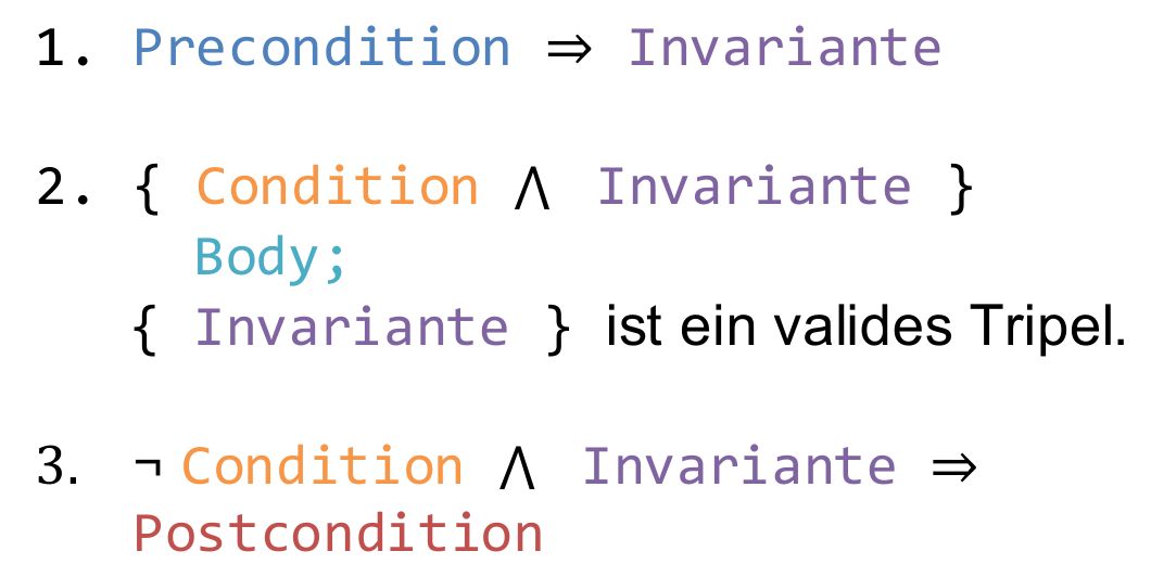
Back
Current
Note has been deleted
Field-by-field Comparison
| Field | Before | After |
|---|---|---|
| Occlusion | ||
| Image |
Note 1114: ETH::1. Semester::EProg
Deck: ETH::1. Semester::EProg
Note Type: Horvath Cloze
GUID:
deleted
Note Type: Horvath Cloze
GUID:
go.nl_(PCT
Deleted Note
Front
The weakest precondition is
true since true only implies true.Back
The weakest precondition is
true since true only implies true.Current
Note has been deleted
Field-by-field Comparison
| Field | Before | After |
|---|---|---|
| Text |
Note 1115: ETH::1. Semester::EProg
Deck: ETH::1. Semester::EProg
Note Type: Horvath Classic
GUID:
deleted
Note Type: Horvath Classic
GUID:
h8y9Gj^3Oz
Deleted Note
Front
Operator precedence in Java for *, /, %, +, -
Back
Operator precedence in Java for *, /, %, +, -
*, /, % bind stronger than +, -
Current
Note has been deleted
Field-by-field Comparison
| Field | Before | After |
|---|---|---|
| Front | ||
| Back |
Note 1116: ETH::1. Semester::EProg
Deck: ETH::1. Semester::EProg
Note Type: Horvath Cloze
GUID:
deleted
Note Type: Horvath Cloze
GUID:
i2g|!nNV|m
Deleted Note
Front
We can omit everything but the semicolons in a for-loop.
Back
We can omit everything but the semicolons in a for-loop.
Current
Note has been deleted
Field-by-field Comparison
| Field | Before | After |
|---|---|---|
| Text |
Note 1117: ETH::1. Semester::EProg
Deck: ETH::1. Semester::EProg
Note Type: Horvath Cloze
GUID:
deleted
Note Type: Horvath Cloze
GUID:
io,]_+ZcUp
Deleted Note
Front
What is the result of:
void test(Integer k) {
k = Integer.valueOf(1); This only changes it locally! (Shadowing)
//
k.value = 1; This changes the value for the caller as well
}
void test(Integer k) {
k = Integer.valueOf(1); This only changes it locally! (Shadowing)
//
k.value = 1; This changes the value for the caller as well
}
Back
What is the result of:
void test(Integer k) {
k = Integer.valueOf(1); This only changes it locally! (Shadowing)
//
k.value = 1; This changes the value for the caller as well
}
void test(Integer k) {
k = Integer.valueOf(1); This only changes it locally! (Shadowing)
//
k.value = 1; This changes the value for the caller as well
}
Current
Note has been deleted
Field-by-field Comparison
| Field | Before | After |
|---|---|---|
| Text |
Note 1118: ETH::1. Semester::EProg
Deck: ETH::1. Semester::EProg
Note Type: Horvath Cloze
GUID:
deleted
Note Type: Horvath Cloze
GUID:
iyK[p{ZDF+
Deleted Note
Front
A a = new B() when calling a.test we get A’s test attribute.Back
A a = new B() when calling a.test we get A’s test attribute.The compiler uses the static type to get attributes.
Current
Note has been deleted
Field-by-field Comparison
| Field | Before | After |
|---|---|---|
| Text | ||
| Extra |
Note 1119: ETH::1. Semester::EProg
Deck: ETH::1. Semester::EProg
Note Type: Horvath Cloze
GUID:
deleted
Note Type: Horvath Cloze
GUID:
iz]M]${2
Deleted Note
Front
Enums have some convenient features:
- can compare using
== - use
.name()to get string representation - go from string to enum using
Status.valueOf("PAID") - Ordering using order in declaration
Status.SUBMITTED < Status.PAID
Back
Enums have some convenient features:
- can compare using
== - use
.name()to get string representation - go from string to enum using
Status.valueOf("PAID") - Ordering using order in declaration
Status.SUBMITTED < Status.PAID
Current
Note has been deleted
Field-by-field Comparison
| Field | Before | After |
|---|---|---|
| Text |
Note 1120: ETH::1. Semester::EProg
Deck: ETH::1. Semester::EProg
Note Type: Horvath Cloze
GUID:
deleted
Note Type: Horvath Cloze
GUID:
j>`+}@t/`y
Deleted Note
Front
class T {
int data = 50;
public void s2() {
System.out.println("T " + data);
}
}
class S extends T {
int data = 100;
public void s2() {
System.out.println(this.data);
}
}
class R extends S {
int data = 200;
}
T r = new R();
r.s2(); // Prints "100"
Back
class T {
int data = 50;
public void s2() {
System.out.println("T " + data);
}
}
class S extends T {
int data = 100;
public void s2() {
System.out.println(this.data);
}
}
class R extends S {
int data = 200;
}
T r = new R();
r.s2(); // Prints "100"
Current
Note has been deleted
Field-by-field Comparison
| Field | Before | After |
|---|---|---|
| Text |
Note 1121: ETH::1. Semester::EProg
Deck: ETH::1. Semester::EProg
Note Type: Horvath Cloze
GUID:
deleted
Note Type: Horvath Cloze
GUID:
jPX[=ewS~@
Deleted Note
Front
EBNF Recursion: Every recursion needs a stop condition.
Back
EBNF Recursion: Every recursion needs a stop condition.
Current
Note has been deleted
Field-by-field Comparison
| Field | Before | After |
|---|---|---|
| Text |
Note 1122: ETH::1. Semester::EProg
Deck: ETH::1. Semester::EProg
Note Type: Horvath Cloze
GUID:
deleted
Note Type: Horvath Cloze
GUID:
m%x4[`&]1%
Deleted Note
Front
Only names and input types determine the signature of a method in Java.
Back
Only names and input types determine the signature of a method in Java.
Current
Note has been deleted
Field-by-field Comparison
| Field | Before | After |
|---|---|---|
| Text |
Note 1123: ETH::1. Semester::EProg
Deck: ETH::1. Semester::EProg
Note Type: Horvath Cloze
GUID:
deleted
Note Type: Horvath Cloze
GUID:
m)$PxVQ^IS
Deleted Note
Front
Zwei EBNF-Beschreibungen sind äquivalent falls ihre Sprachen gleich sind.
Back
Zwei EBNF-Beschreibungen sind äquivalent falls ihre Sprachen gleich sind.
Current
Note has been deleted
Field-by-field Comparison
| Field | Before | After |
|---|---|---|
| Text |
Note 1124: ETH::1. Semester::EProg
Deck: ETH::1. Semester::EProg
Note Type: Horvath Cloze
GUID:
deleted
Note Type: Horvath Cloze
GUID:
m5.*#}3,2{
Deleted Note
Front
Possible casting problems:
- String s = (String) new Integer(5); Casting between unrelated classes
- Animal a2 = new Cat(); Dog d2 = (Dog) a2; ClassCastException!
Back
Possible casting problems:
- String s = (String) new Integer(5); Casting between unrelated classes
- Animal a2 = new Cat(); Dog d2 = (Dog) a2; ClassCastException!
Current
Note has been deleted
Field-by-field Comparison
| Field | Before | After |
|---|---|---|
| Text |
Note 1125: ETH::1. Semester::EProg
Deck: ETH::1. Semester::EProg
Note Type: Horvath Cloze
GUID:
deleted
Note Type: Horvath Cloze
GUID:
mxWnHn=6?K
Deleted Note
Front
Unchecked exceptions can but don't have to be caught.
Back
Unchecked exceptions can but don't have to be caught.
Current
Note has been deleted
Field-by-field Comparison
| Field | Before | After |
|---|---|---|
| Text |
Note 1126: ETH::1. Semester::EProg
Deck: ETH::1. Semester::EProg
Note Type: Horvath Cloze
GUID:
deleted
Note Type: Horvath Cloze
GUID:
m{lpYbESok
Deleted Note
Front
If we set the reference to an array to null inside a function, the caller still has the reference, as it's copied.
Back
If we set the reference to an array to null inside a function, the caller still has the reference, as it's copied.
Current
Note has been deleted
Field-by-field Comparison
| Field | Before | After |
|---|---|---|
| Text |
Note 1127: ETH::1. Semester::EProg
Deck: ETH::1. Semester::EProg
Note Type: Horvath Cloze
GUID:
deleted
Note Type: Horvath Cloze
GUID:
o!E/h>2m7B
Deleted Note
Front
Private attributes cannot be accessed in subclasses, but we can still access them as a user through non-overriden methods.
Back
Private attributes cannot be accessed in subclasses, but we can still access them as a user through non-overriden methods.
Current
Note has been deleted
Field-by-field Comparison
| Field | Before | After |
|---|---|---|
| Text |
Note 1128: ETH::1. Semester::EProg
Deck: ETH::1. Semester::EProg
Note Type: Horvath Cloze
GUID:
deleted
Note Type: Horvath Cloze
GUID:
o#o/7wH;E.
Deleted Note
Front
The convention for EBNF is that the rule being considered is written last.
Back
The convention for EBNF is that the rule being considered is written last.
Current
Note has been deleted
Field-by-field Comparison
| Field | Before | After |
|---|---|---|
| Text |
Note 1129: ETH::1. Semester::EProg
Deck: ETH::1. Semester::EProg
Note Type: Horvath Cloze
GUID:
deleted
Note Type: Horvath Cloze
GUID:
o2_oVlzFE[
Deleted Note
Front
To compare two strings (or any non-primite type) we use .equals() .
Back
To compare two strings (or any non-primite type) we use .equals() .
== compares the references, not the values.
Current
Note has been deleted
Field-by-field Comparison
| Field | Before | After |
|---|---|---|
| Text | ||
| Extra |
Note 1130: ETH::1. Semester::EProg
Deck: ETH::1. Semester::EProg
Note Type: Horvath Classic
GUID:
deleted
Note Type: Horvath Classic
GUID:
o5fc<3#h._
Deleted Note
Front
What does 5 % 0 produce in Java?
Back
What does 5 % 0 produce in Java?
Runtime error, division by 0
Current
Note has been deleted
Field-by-field Comparison
| Field | Before | After |
|---|---|---|
| Front | ||
| Back |
Note 1131: ETH::1. Semester::EProg
Deck: ETH::1. Semester::EProg
Note Type: Horvath Classic
GUID:
deleted
Note Type: Horvath Classic
GUID:
oCoi_,?<4<
Deleted Note
Front
x++ does what?
Back
x++ does what?
Returns x then increments by one.
Current
Note has been deleted
Field-by-field Comparison
| Field | Before | After |
|---|---|---|
| Front | ||
| Back |
Note 1132: ETH::1. Semester::EProg
Deck: ETH::1. Semester::EProg
Note Type: Horvath Cloze
GUID:
deleted
Note Type: Horvath Cloze
GUID:
oE~TL)}ZNN
Deleted Note
Front
In Java a class cannot inherit from multiple super-classes.
Back
In Java a class cannot inherit from multiple super-classes.
This works only for interfaces.
Current
Note has been deleted
Field-by-field Comparison
| Field | Before | After |
|---|---|---|
| Text | ||
| Extra |
Note 1133: ETH::1. Semester::EProg
Deck: ETH::1. Semester::EProg
Note Type: Horvath Cloze
GUID:
deleted
Note Type: Horvath Cloze
GUID:
oWLG{z90=/
Deleted Note
Front
To initialise an array directly we use int[] test = {{c1:: {1, 2, 3 ...};}}.
Back
To initialise an array directly we use int[] test = {{c1:: {1, 2, 3 ...};}}.
Current
Note has been deleted
Field-by-field Comparison
| Field | Before | After |
|---|---|---|
| Text |
Note 1134: ETH::1. Semester::EProg
Deck: ETH::1. Semester::EProg
Note Type: Horvath Classic
GUID:
deleted
Note Type: Horvath Classic
GUID:
osPOmm:i4.
Deleted Note
Front
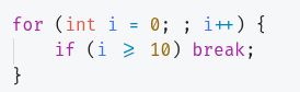
Compile/Runtime/No Error
Back
Compile/Runtime/No Error
No error, valid for-loop.
Current
Note has been deleted
Field-by-field Comparison
| Field | Before | After |
|---|---|---|
| Front | ||
| Back |
Note 1135: ETH::1. Semester::EProg
Deck: ETH::1. Semester::EProg
Note Type: Horvath Cloze
GUID:
deleted
Note Type: Horvath Cloze
GUID:
p$+y{A-`_b
Deleted Note
Front
Casts from int to long and double can always be implicit.
Back
Casts from int to long and double can always be implicit.
Current
Note has been deleted
Field-by-field Comparison
| Field | Before | After |
|---|---|---|
| Text |
Note 1136: ETH::1. Semester::EProg
Deck: ETH::1. Semester::EProg
Note Type: Horvath Cloze
GUID:
deleted
Note Type: Horvath Cloze
GUID:
p,3.jh@oZC
Deleted Note
Front
Shadowing is when an inner scope variable makes an outer scope one inaccessible.
Back
Shadowing is when an inner scope variable makes an outer scope one inaccessible.
public class Person {
private String name; // instance variable
public void setName(String name) { // parameter shadows instance variable
this.name = name; // use 'this' to access the instance variable
}
}
private String name; // instance variable
public void setName(String name) { // parameter shadows instance variable
this.name = name; // use 'this' to access the instance variable
}
}
Current
Note has been deleted
Field-by-field Comparison
| Field | Before | After |
|---|---|---|
| Text | ||
| Extra |
Note 1137: ETH::1. Semester::EProg
Deck: ETH::1. Semester::EProg
Note Type: Horvath Cloze
GUID:
deleted
Note Type: Horvath Cloze
GUID:
p1.Wet4$5I
Deleted Note
Front
If we see "((C) D).something()" as a cast we can assume that D is a subtype of C.
Back
If we see "((C) D).something()" as a cast we can assume that D is a subtype of C.
This is relevant for EProg theory exercises in which we have to reconstruct a class hierarchy.
Current
Note has been deleted
Field-by-field Comparison
| Field | Before | After |
|---|---|---|
| Text | ||
| Extra |
Note 1138: ETH::1. Semester::EProg
Deck: ETH::1. Semester::EProg
Note Type: Horvath Cloze
GUID:
deleted
Note Type: Horvath Cloze
GUID:
p9%v,4EY(!
Deleted Note
Front
Values given to a method in Java are always copied.
Back
Values given to a method in Java are always copied.
Current
Note has been deleted
Field-by-field Comparison
| Field | Before | After |
|---|---|---|
| Text |
Note 1139: ETH::1. Semester::EProg
Deck: ETH::1. Semester::EProg
Note Type: Horvath Classic
GUID:
deleted
Note Type: Horvath Classic
GUID:
pD;qk4geEz
Deleted Note
Front
The output of this code snippet is:
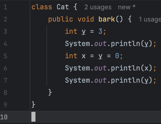
Back
The output of this code snippet is:
3
0
0
0
0
Current
Note has been deleted
Field-by-field Comparison
| Field | Before | After |
|---|---|---|
| Front | ||
| Back |
Note 1140: ETH::1. Semester::EProg
Deck: ETH::1. Semester::EProg
Note Type: Horvath Classic
GUID:
deleted
Note Type: Horvath Classic
GUID:
pycoxP)lJk
Deleted Note
Front
10 / -2 in Java gives the result 5 or -5?
Back
10 / -2 in Java gives the result 5 or -5?
-5 as integer division also supports negatives.
Current
Note has been deleted
Field-by-field Comparison
| Field | Before | After |
|---|---|---|
| Front | ||
| Back |
Note 1141: ETH::1. Semester::EProg
Deck: ETH::1. Semester::EProg
Note Type: Horvath Cloze
GUID:
deleted
Note Type: Horvath Cloze
GUID:
q+A$0CHp#W
Deleted Note
Front
If we override an attribute inherited from the parentclass, it will override the parents attribute.
Back
If we override an attribute inherited from the parentclass, it will override the parents attribute.
class A {
public int x = 5;
public void fct1() {
System.out.println(this.x);
}
}
class B extends A {
public B() {
super.x = 10;
}
public B(int a) {
super.x = a;
}
}
A a1 = new B(1);
A a2 = new B(12); // As these are different instances, their attributes are separate
B b1 = new B(1);
B b2 = new B(12);
a1.fct1(); // 1 -> Even though static type is A
a2.fct1(); // 12 -> Different output as a2's instance of A has 12
b1.fct1(); // 1 -> same here, even though it dynamic dispatches
b2.fct1(); // 12
Current
Note has been deleted
Field-by-field Comparison
| Field | Before | After |
|---|---|---|
| Text | ||
| Extra |
Note 1142: ETH::1. Semester::EProg
Deck: ETH::1. Semester::EProg
Note Type: Horvath Cloze
GUID:
deleted
Note Type: Horvath Cloze
GUID:
qj}+Vy$^iX
Deleted Note
Front
In an interface:
- All methods are public (doesn’t have to be explicit).
- Any attributes must be public and final.
Back
In an interface:
- All methods are public (doesn’t have to be explicit).
- Any attributes must be public and final.
Current
Note has been deleted
Field-by-field Comparison
| Field | Before | After |
|---|---|---|
| Text |
Note 1143: ETH::1. Semester::EProg
Deck: ETH::1. Semester::EProg
Note Type: Horvath Classic
GUID:
deleted
Note Type: Horvath Classic
GUID:
q|N{Bb]-?+
Deleted Note
Front
// {P}
if (a) {
S1;
} else {
S2;
}
// {Q}
Back
// {P}
if (a) {
S1;
} else {
S2;
}
// {Q}
Man muss zwei Fälle checken:
- \(P \land a \implies Q\) when S1; is executed.
- \(P \land \lnot a \implies Q\) when S2; is executed.
a && precondition1 OR !a && precondition2Current
Note has been deleted
Field-by-field Comparison
| Field | Before | After |
|---|---|---|
| Front | ||
| Back |
Note 1144: ETH::1. Semester::EProg
Deck: ETH::1. Semester::EProg
Note Type: Horvath Cloze
GUID:
deleted
Note Type: Horvath Cloze
GUID:
rcu~6HwhWg
Deleted Note
Front
Static methods can only access static attributes.
Back
Static methods can only access static attributes.
Current
Note has been deleted
Field-by-field Comparison
| Field | Before | After |
|---|---|---|
| Text |
Note 1145: ETH::1. Semester::EProg
Deck: ETH::1. Semester::EProg
Note Type: Horvath Cloze
GUID:
deleted
Note Type: Horvath Cloze
GUID:
rd5%P7v`6L
Deleted Note
Front
If
P_1 implies P_2 then we can say that P_1 is a stronger precondition than P_2.Back
If
P_1 implies P_2 then we can say that P_1 is a stronger precondition than P_2.Current
Note has been deleted
Field-by-field Comparison
| Field | Before | After |
|---|---|---|
| Text |
Note 1146: ETH::1. Semester::EProg
Deck: ETH::1. Semester::EProg
Note Type: Horvath Cloze
GUID:
deleted
Note Type: Horvath Cloze
GUID:
rz>>y0Yl@}
Deleted Note
Front
An unchecked exception extends RuntimeException and does not need to be announced nor caught.
Back
An unchecked exception extends RuntimeException and does not need to be announced nor caught.
Current
Note has been deleted
Field-by-field Comparison
| Field | Before | After |
|---|---|---|
| Text |
Note 1147: ETH::1. Semester::EProg
Deck: ETH::1. Semester::EProg
Note Type: Horvath Classic
GUID:
deleted
Note Type: Horvath Classic
GUID:
s*V3JSYg7q
Deleted Note
Front
Name the EBNF Precedence rules
Back
Name the EBNF Precedence rules
- selection / option / repetition
- sequence (weaker than everything else)
Current
Note has been deleted
Field-by-field Comparison
| Field | Before | After |
|---|---|---|
| Front | ||
| Back |
Note 1148: ETH::1. Semester::EProg
Deck: ETH::1. Semester::EProg
Note Type: Horvath Cloze
GUID:
deleted
Note Type: Horvath Cloze
GUID:
sC;1?2R2yM
Deleted Note
Front
String s = "test"; to acces the first character we use s.charAt(0).
Back
String s = "test"; to acces the first character we use s.charAt(0).
Current
Note has been deleted
Field-by-field Comparison
| Field | Before | After |
|---|---|---|
| Text |
Note 1149: ETH::1. Semester::EProg
Deck: ETH::1. Semester::EProg
Note Type: Horvath Cloze
GUID:
deleted
Note Type: Horvath Cloze
GUID:
sV73UB+t=%
Deleted Note
Front
An interface can extend another interface.
Back
An interface can extend another interface.
Note that it extends not implements it.
Current
Note has been deleted
Field-by-field Comparison
| Field | Before | After |
|---|---|---|
| Text | ||
| Extra |
Note 1150: ETH::1. Semester::EProg
Deck: ETH::1. Semester::EProg
Note Type: Horvath Cloze
GUID:
deleted
Note Type: Horvath Cloze
GUID:
s[]2mb-kIp
Deleted Note
Front
We can change the static type of a variable by casting.
Back
We can change the static type of a variable by casting.
Current
Note has been deleted
Field-by-field Comparison
| Field | Before | After |
|---|---|---|
| Text |
Note 1151: ETH::1. Semester::EProg
Deck: ETH::1. Semester::EProg
Note Type: Horvath Cloze
GUID:
deleted
Note Type: Horvath Cloze
GUID:
t;7tcil{&|
Deleted Note
Front
An EBNF rule is defined by writing a variable name wrapped in < >.
Back
An EBNF rule is defined by writing a variable name wrapped in < >.
Current
Note has been deleted
Field-by-field Comparison
| Field | Before | After |
|---|---|---|
| Text |
Note 1152: ETH::1. Semester::EProg
Deck: ETH::1. Semester::EProg
Note Type: Horvath Classic
GUID:
deleted
Note Type: Horvath Classic
GUID:
t=MANr.EfE
Deleted Note
Front
What is the weakest precondition for an empty program with postcondition
true?Back
What is the weakest precondition for an empty program with postcondition
true?true.
Everything implies true and true implies true.
Everything implies true and true implies true.
Current
Note has been deleted
Field-by-field Comparison
| Field | Before | After |
|---|---|---|
| Front | ||
| Back |
Note 1153: ETH::1. Semester::EProg
Deck: ETH::1. Semester::EProg
Note Type: Horvath Classic
GUID:
deleted
Note Type: Horvath Classic
GUID:
tja~6C@vsv
Deleted Note
Front
Does Java enforce array dimensions using type- or runtime-checks?
Back
Does Java enforce array dimensions using type- or runtime-checks?
No, this is fine:
int[][] b = new int[3][0];int[] c = new int[3]; b[0] = c;Current
Note has been deleted
Field-by-field Comparison
| Field | Before | After |
|---|---|---|
| Front | ||
| Back |
Note 1154: ETH::1. Semester::EProg
Deck: ETH::1. Semester::EProg
Note Type: Horvath Cloze
GUID:
deleted
Note Type: Horvath Cloze
GUID:
uD7<2m5W}k
Deleted Note
Front
Java has short circuiting for the && and || operators.
This means that if the left of
- && is false then the right isn't even executed
- || is true then the right isn't even executed
Keep this in mind if there's a runtime error on the right.
Back
Java has short circuiting for the && and || operators.
This means that if the left of
- && is false then the right isn't even executed
- || is true then the right isn't even executed
Keep this in mind if there's a runtime error on the right.
Current
Note has been deleted
Field-by-field Comparison
| Field | Before | After |
|---|---|---|
| Text |
Note 1155: ETH::1. Semester::EProg
Deck: ETH::1. Semester::EProg
Note Type: Horvath Cloze
GUID:
deleted
Note Type: Horvath Cloze
GUID:
uG5r)XSwb;
Deleted Note
Front
Java "=" is right-associative
Back
Java "=" is right-associative
a = b = c = 5 means all are equal to 5.
Current
Note has been deleted
Field-by-field Comparison
| Field | Before | After |
|---|---|---|
| Text | ||
| Extra |
Note 1156: ETH::1. Semester::EProg
Deck: ETH::1. Semester::EProg
Note Type: Horvath Cloze
GUID:
deleted
Note Type: Horvath Cloze
GUID:
v:4|0s-7ML
Deleted Note
Front
All implementations of an interface using
implements must instantiate all methods declared by the interface , otherwise we get a compiler error.Back
All implementations of an interface using
implements must instantiate all methods declared by the interface , otherwise we get a compiler error.(except if the class is abstract, then we don't have to implement them)
Current
Note has been deleted
Field-by-field Comparison
| Field | Before | After |
|---|---|---|
| Text | ||
| Extra |
Note 1157: ETH::1. Semester::EProg
Deck: ETH::1. Semester::EProg
Note Type: Horvath Cloze
GUID:
deleted
Note Type: Horvath Cloze
GUID:
v]c0VE0GBF
Deleted Note
Front
1 + "" results in "1" in Java.
Back
1 + "" results in "1" in Java.
+ "" will cast anything via .toString().
Current
Note has been deleted
Field-by-field Comparison
| Field | Before | After |
|---|---|---|
| Text | ||
| Extra |
Note 1158: ETH::1. Semester::EProg
Deck: ETH::1. Semester::EProg
Note Type: Horvath Cloze
GUID:
deleted
Note Type: Horvath Cloze
GUID:
vzp2j2|98!
Deleted Note
Front
Order of EBNF rules does not matter.
Back
Order of EBNF rules does not matter.
Current
Note has been deleted
Field-by-field Comparison
| Field | Before | After |
|---|---|---|
| Text |
Note 1159: ETH::1. Semester::EProg
Deck: ETH::1. Semester::EProg
Note Type: Horvath Cloze
GUID:
deleted
Note Type: Horvath Cloze
GUID:
w3Z$4;rQou
Deleted Note
Front
We cannot instantiate abstract classes and interfaces.
Back
We cannot instantiate abstract classes and interfaces.
Current
Note has been deleted
Field-by-field Comparison
| Field | Before | After |
|---|---|---|
| Text |
Note 1160: ETH::1. Semester::EProg
Deck: ETH::1. Semester::EProg
Note Type: Horvath Cloze
GUID:
deleted
Note Type: Horvath Cloze
GUID:
w5QXs;%q{4
Deleted Note
Front
Ein Symbol (auf der RHS) wie z.B. 1, a, A in EBNF wird Terminal oder auch Literal gennant.
Back
Ein Symbol (auf der RHS) wie z.B. 1, a, A in EBNF wird Terminal oder auch Literal gennant.
Current
Note has been deleted
Field-by-field Comparison
| Field | Before | After |
|---|---|---|
| Text |
Note 1161: ETH::1. Semester::EProg
Deck: ETH::1. Semester::EProg
Note Type: Horvath Cloze
GUID:
deleted
Note Type: Horvath Cloze
GUID:
wT:
Deleted Note
Front
In EBNF we can write a recursive rule by writing the rule name on both sides e.g. <A> \(\leftarrow\) A[<A>] or by writing a series of rules that result in the same.
Back
In EBNF we can write a recursive rule by writing the rule name on both sides e.g. <A> \(\leftarrow\) A[<A>] or by writing a series of rules that result in the same.
Current
Note has been deleted
Field-by-field Comparison
| Field | Before | After |
|---|---|---|
| Text |
Note 1162: ETH::1. Semester::EProg
Deck: ETH::1. Semester::EProg
Note Type: Horvath Cloze
GUID:
deleted
Note Type: Horvath Cloze
GUID:
xnz4`TH(j}
Deleted Note
Front
What methods cannot be overriden in a subclass:
staticfinalprivateare not inherited eitherconstructors
Back
What methods cannot be overriden in a subclass:
staticfinalprivateare not inherited eitherconstructors
Current
Note has been deleted
Field-by-field Comparison
| Field | Before | After |
|---|---|---|
| Text |
Note 1163: ETH::1. Semester::EProg
Deck: ETH::1. Semester::EProg
Note Type: Horvath Classic
GUID:
deleted
Note Type: Horvath Classic
GUID:
x}m)l,UDD1
Deleted Note
Front
int x = 2;
++x + x++;
evaluates to ???
++x + x++;
evaluates to ???
Back
int x = 2;
++x + x++;
evaluates to ???
++x + x++;
evaluates to ???
x = 6
Current
Note has been deleted
Field-by-field Comparison
| Field | Before | After |
|---|---|---|
| Front | ||
| Back |
Note 1164: ETH::1. Semester::EProg
Deck: ETH::1. Semester::EProg
Note Type: Horvath Cloze
GUID:
deleted
Note Type: Horvath Cloze
GUID:
yNOkeWyJB3
Deleted Note
Front
The strongest precondition is
false since it implies everything.Back
The strongest precondition is
false since it implies everything.Current
Note has been deleted
Field-by-field Comparison
| Field | Before | After |
|---|---|---|
| Text |
Note 1165: ETH::1. Semester::EProg
Deck: ETH::1. Semester::EProg
Note Type: Horvath Classic
GUID:
deleted
Note Type: Horvath Classic
GUID:
yf1!;I`$7~
Deleted Note
Front
What does -11 % 4 evaluate to in Java?
Back
What does -11 % 4 evaluate to in Java?
-3
Current
Note has been deleted
Field-by-field Comparison
| Field | Before | After |
|---|---|---|
| Front | ||
| Back |
Note 1166: ETH::1. Semester::EProg
Deck: ETH::1. Semester::EProg
Note Type: Horvath Cloze
GUID:
deleted
Note Type: Horvath Cloze
GUID:
yj/5Ksg%P1
Deleted Note
Front
A static attribute is unique amongst all imports. If we don't make it final it can be changed globally.
Back
A static attribute is unique amongst all imports. If we don't make it final it can be changed globally.
This means someone could change Math.PI for example.
Current
Note has been deleted
Field-by-field Comparison
| Field | Before | After |
|---|---|---|
| Text | ||
| Extra |
Note 1167: ETH::1. Semester::EProg
Deck: ETH::1. Semester::EProg
Note Type: Horvath Cloze
GUID:
deleted
Note Type: Horvath Cloze
GUID:
yrm.]7QjhX
Deleted Note
Front
A static method cannot access this or other non-static class methods.
Back
A static method cannot access this or other non-static class methods.
Current
Note has been deleted
Field-by-field Comparison
| Field | Before | After |
|---|---|---|
| Text |
Note 1168: ETH::1. Semester::EProg
Deck: ETH::1. Semester::EProg
Note Type: Horvath Cloze
GUID:
deleted
Note Type: Horvath Cloze
GUID:
y}<[=^7@`S
Deleted Note
Front
interface B {
Object getValue();
void process() throws IOException;
}
interface A extends B {
// 1. Covariant return type - more specific than Object
String getValue();
// Valid override
// 2. Can reduce or eliminate exceptions
void process();
// Valid - removes IOException
// 3. Can add default implementation
default String getValue() {
return "default";
}
}
Back
interface B {
Object getValue();
void process() throws IOException;
}
interface A extends B {
// 1. Covariant return type - more specific than Object
String getValue();
// Valid override
// 2. Can reduce or eliminate exceptions
void process();
// Valid - removes IOException
// 3. Can add default implementation
default String getValue() {
return "default";
}
}
Current
Note has been deleted
Field-by-field Comparison
| Field | Before | After |
|---|---|---|
| Text |
Note 1169: ETH::1. Semester::EProg
Deck: ETH::1. Semester::EProg
Note Type: Horvath Cloze
GUID:
deleted
Note Type: Horvath Cloze
GUID:
z*_4p
Deleted Note
Front
The Object type defines:
- .equals(Object o)
- .toString()
Back
The Object type defines:
- .equals(Object o)
- .toString()
Current
Note has been deleted
Field-by-field Comparison
| Field | Before | After |
|---|---|---|
| Text |
Note 1170: ETH::1. Semester::EProg
Deck: ETH::1. Semester::EProg
Note Type: Horvath Cloze
GUID:
deleted
Note Type: Horvath Cloze
GUID:
z3M|&J1r.r
Deleted Note
Front
Not every EBNF language (Sprache) can be described just with repetition (Wiederholung).
Back
Not every EBNF language (Sprache) can be described just with repetition (Wiederholung).
Current
Note has been deleted
Field-by-field Comparison
| Field | Before | After |
|---|---|---|
| Text |
Note 1171: ETH::1. Semester::EProg
Deck: ETH::1. Semester::EProg
Note Type: Horvath Cloze
GUID:
deleted
Note Type: Horvath Cloze
GUID:
z=94+q]*#%
Deleted Note
Front
Any type is a subtype of the Object type.
Back
Any type is a subtype of the Object type.
Current
Note has been deleted
Field-by-field Comparison
| Field | Before | After |
|---|---|---|
| Text |
Note 1172: ETH::1. Semester::EProg
Deck: ETH::1. Semester::EProg
Note Type: Horvath Cloze
GUID:
deleted
Note Type: Horvath Cloze
GUID:
zCPO7,.L4T
Deleted Note
Front
A Java identifier can only include lower- and uppercase letters and digits and may never start with digits.
Back
A Java identifier can only include lower- and uppercase letters and digits and may never start with digits.
Current
Note has been deleted
Field-by-field Comparison
| Field | Before | After |
|---|---|---|
| Text |
Note 1173: ETH::1. Semester::LinAlg
Deck: ETH::1. Semester::LinAlg
Note Type: Horvath Cloze
GUID:
deleted
Note Type: Horvath Cloze
GUID:
(scS~v1D#
Deleted Note
Front
\((AB)^{\top}=\)\(B^\top A^\top\)
Back
\((AB)^{\top}=\)\(B^\top A^\top\)
Current
Note has been deleted
Field-by-field Comparison
| Field | Before | After |
|---|---|---|
| Text |
Note 1174: ETH::1. Semester::LinAlg
Deck: ETH::1. Semester::LinAlg
Note Type: Horvath Classic
GUID:
deleted
Note Type: Horvath Classic
GUID:
(wR19U.@d
Deleted Note
Front
What is the result of \(\textbf{0} \cdot \textbf{v}\)
Back
What is the result of \(\textbf{0} \cdot \textbf{v}\)
It is 0, thus 0 is orthogonal to all vectors.
Current
Note has been deleted
Field-by-field Comparison
| Field | Before | After |
|---|---|---|
| Front | ||
| Back |
Note 1175: ETH::1. Semester::LinAlg
Deck: ETH::1. Semester::LinAlg
Note Type: Horvath Cloze
GUID:
deleted
Note Type: Horvath Cloze
GUID:
A.Z_4&Nx-g
Deleted Note
Front
Given \(A \in \mathbb{R}^{n \times n}\) we say \(\lambda \in \mathbb{C}\) is an eigenvalue of \(A\) and \(v \in \mathbb{C}^{n} \setminus \{0\}\) is an eigenvector of \(A\) associated with the eigenvalue \(\lambda\) when the following holds: \[ Av = \lambda v \]
Back
Given \(A \in \mathbb{R}^{n \times n}\) we say \(\lambda \in \mathbb{C}\) is an eigenvalue of \(A\) and \(v \in \mathbb{C}^{n} \setminus \{0\}\) is an eigenvector of \(A\) associated with the eigenvalue \(\lambda\) when the following holds: \[ Av = \lambda v \]
Current
Note has been deleted
Field-by-field Comparison
| Field | Before | After |
|---|---|---|
| Text |
Note 1176: ETH::1. Semester::LinAlg
Deck: ETH::1. Semester::LinAlg
Note Type: Horvath Cloze
GUID:
deleted
Note Type: Horvath Cloze
GUID:
A7le9*7QY+
Deleted Note
Front
The eigenvectors of \(A^{-1}\) are the same as those of \(A\).
Back
The eigenvectors of \(A^{-1}\) are the same as those of \(A\).
Current
Note has been deleted
Field-by-field Comparison
| Field | Before | After |
|---|---|---|
| Text |
Note 1177: ETH::1. Semester::LinAlg
Deck: ETH::1. Semester::LinAlg
Note Type: Horvath Cloze
GUID:
deleted
Note Type: Horvath Cloze
GUID:
AA?D}V$bUJ
Deleted Note
Front
The output of Gauss-Jordan on a matrix \(A\) is unique.
Back
The output of Gauss-Jordan on a matrix \(A\) is unique.
Current
Note has been deleted
Field-by-field Comparison
| Field | Before | After |
|---|---|---|
| Text |
Note 1178: ETH::1. Semester::LinAlg
Deck: ETH::1. Semester::LinAlg
Note Type: Horvath Cloze
GUID:
deleted
Note Type: Horvath Cloze
GUID:
AG3+NsB]T%
Deleted Note
Front
\(\mathbb{R}^{m \times n}\) is not actually a new vector space, it is isomorphic to {{c1::\(\mathbb{R}^{m \cdot n}\)}}.
Back
\(\mathbb{R}^{m \times n}\) is not actually a new vector space, it is isomorphic to {{c1::\(\mathbb{R}^{m \cdot n}\)}}.
Current
Note has been deleted
Field-by-field Comparison
| Field | Before | After |
|---|---|---|
| Text |
Note 1179: ETH::1. Semester::LinAlg
Deck: ETH::1. Semester::LinAlg
Note Type: Horvath Cloze
GUID:
deleted
Note Type: Horvath Cloze
GUID:
AN(F>bO#!5
Deleted Note
Front
The matrix \(A^k\) has EW-EV pair \(\lambda^k\) and \(v\) if \(A\) has \(\lambda, v\) as an EW-EV pair.
Back
The matrix \(A^k\) has EW-EV pair \(\lambda^k\) and \(v\) if \(A\) has \(\lambda, v\) as an EW-EV pair.
Intuitively, \(A\) on \(v\) scales it by \(\lambda\). Then scaling that already scaled \(\lambda v\) by \(A\) again gives us \(\lambda^2 v\), etc...
Current
Note has been deleted
Field-by-field Comparison
| Field | Before | After |
|---|---|---|
| Text | ||
| Extra |
Note 1180: ETH::1. Semester::LinAlg
Deck: ETH::1. Semester::LinAlg
Note Type: Horvath Cloze
GUID:
deleted
Note Type: Horvath Cloze
GUID:
AR!ygs@:}2
Deleted Note
Front
The error vector is orthogonal to the projection.
Back
The error vector is orthogonal to the projection.
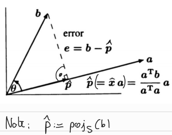
Current
Note has been deleted
Field-by-field Comparison
| Field | Before | After |
|---|---|---|
| Text | ||
| Extra |
Note 1181: ETH::1. Semester::LinAlg
Deck: ETH::1. Semester::LinAlg
Note Type: Horvath Classic
GUID:
deleted
Note Type: Horvath Classic
GUID:
AXk(.4O|pc
Deleted Note
Front
Why is \(R\) upper triangular in the QR decomposition?
Back
Why is \(R\) upper triangular in the QR decomposition?
\(R\) is upper triangular because each \(q_k\) is orthogonal to every \(a_i\) for \(i < k\) (all after it), thus they are \(0\).
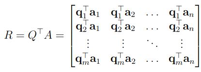
You can see here, since \(q_2, \dots, q_m\) are by construction orthogonal to \(q_1\) thus \(a_1\), all entries below \(1\) in the first column are \(0\). The same goes for all entries below \(2\) in the second column.
You can see here, since \(q_2, \dots, q_m\) are by construction orthogonal to \(q_1\) thus \(a_1\), all entries below \(1\) in the first column are \(0\). The same goes for all entries below \(2\) in the second column.
Current
Note has been deleted
Field-by-field Comparison
| Field | Before | After |
|---|---|---|
| Front | ||
| Back |
Note 1182: ETH::1. Semester::LinAlg
Deck: ETH::1. Semester::LinAlg
Note Type: Horvath Cloze
GUID:
deleted
Note Type: Horvath Cloze
GUID:
AZx@62[!CP
Deleted Note
Front
Let \(A\) be an invertible matrix. If \(\lambda\) and \(v\) are an EW-EV pair, then {{c1:: \(\frac{1}{\lambda}\) and \(v\)}} are an EW-EV pair of the matrix \(A^{-1}\). Proof Included
Back
Let \(A\) be an invertible matrix. If \(\lambda\) and \(v\) are an EW-EV pair, then {{c1:: \(\frac{1}{\lambda}\) and \(v\)}} are an EW-EV pair of the matrix \(A^{-1}\). Proof Included
Proof: We have \(Av = \lambda v\) thus \(A^{-1}Av = \lambda A^{-1}v\) thus \(\frac{1}{\lambda} v = \frac{1}{\lambda} \lambda A^{-1}v\) and we get \(A^{-1}v = \frac{1}{\lambda} v\).
Current
Note has been deleted
Field-by-field Comparison
| Field | Before | After |
|---|---|---|
| Text | ||
| Extra |
Note 1183: ETH::1. Semester::LinAlg
Deck: ETH::1. Semester::LinAlg
Note Type: Horvath Cloze
GUID:
deleted
Note Type: Horvath Cloze
GUID:
A[sn#o|@++
Deleted Note
Front
A vector space \(V\) over a field \(F\) is a set with vector addition (\(V \times V \mapsto V)\) and scalar multiplication (\(F \times V \mapsto V\)) being defined. The elements of \(V\) are then usually called vectors and the elements of \(F\) scalars.
Back
A vector space \(V\) over a field \(F\) is a set with vector addition (\(V \times V \mapsto V)\) and scalar multiplication (\(F \times V \mapsto V\)) being defined. The elements of \(V\) are then usually called vectors and the elements of \(F\) scalars.
Example: \(\mathbb{R}^2\) with the usual definitions of \(+, \cdot\) (cartesian vectors)
Current
Note has been deleted
Field-by-field Comparison
| Field | Before | After |
|---|---|---|
| Text | ||
| Extra |
Note 1184: ETH::1. Semester::LinAlg
Deck: ETH::1. Semester::LinAlg
Note Type: Horvath Classic
GUID:
deleted
Note Type: Horvath Classic
GUID:
Ai8Yhc45CL
Deleted Note
Front
How do we compute a basis for \(C(A)\)?
Back
How do we compute a basis for \(C(A)\)?
The independent columns in the RREF form of matrix \(A\) are a basis of the column space and in particular: \(\dim(\textbf{C}(A)) = \textbf{rank}(A) = r\)
Current
Note has been deleted
Field-by-field Comparison
| Field | Before | After |
|---|---|---|
| Front | ||
| Back |
Note 1185: ETH::1. Semester::LinAlg
Deck: ETH::1. Semester::LinAlg
Note Type: Horvath Cloze
GUID:
deleted
Note Type: Horvath Cloze
GUID:
Ap,1=OrtVQ
Deleted Note
Front
\[ P(z) = (-1)^n \det(A - z I) = \det(z I - A) = (z - \lambda_1)(z - \lambda_2) \dots (z - \lambda_n) \]
The polynomial \(P(z)\) is called the characteristic polynomial of the matrix \(A\).
Back
\[ P(z) = (-1)^n \det(A - z I) = \det(z I - A) = (z - \lambda_1)(z - \lambda_2) \dots (z - \lambda_n) \]
The polynomial \(P(z)\) is called the characteristic polynomial of the matrix \(A\).
The eigenvalues \(\lambda_1, \dots, \lambda_n\) as they show up in the polynomial are not all distinct in general.
The number of times an eigenvalue shows up is called the algebraic multiplicity of the eigenvalue.
Current
Note has been deleted
Field-by-field Comparison
| Field | Before | After |
|---|---|---|
| Text | ||
| Extra |
Note 1186: ETH::1. Semester::LinAlg
Deck: ETH::1. Semester::LinAlg
Note Type: Horvath Cloze
GUID:
deleted
Note Type: Horvath Cloze
GUID:
Ar}c<-r5#~
Deleted Note
Front
Orthogonal matrices preserve the norm and inner product of vectors.
Back
Orthogonal matrices preserve the norm and inner product of vectors.
In other words, if \(Q \in \mathbb{R}^{n \times n}\) is orthogonal, then, for all \(x, y \in \mathbb{R}^n\):
\[ ||Qx|| = ||x|| \text{ and } (Qx)^\top(Qy) = x^\top y \]
\[ ||Qx|| = ||x|| \text{ and } (Qx)^\top(Qy) = x^\top y \]
Current
Note has been deleted
Field-by-field Comparison
| Field | Before | After |
|---|---|---|
| Text | ||
| Extra |
Note 1187: ETH::1. Semester::LinAlg
Deck: ETH::1. Semester::LinAlg
Note Type: Horvath Cloze
GUID:
deleted
Note Type: Horvath Cloze
GUID:
Az@K^QzYw.
Deleted Note
Front
A symmetric matrix \(A \in \mathbb{R}^{n \times n}\) is positive semidefinite if and only if {{c2::\(x^\top A x \geq 0\) for all \(x \in \mathbb{R}^n\)}}.
Back
A symmetric matrix \(A \in \mathbb{R}^{n \times n}\) is positive semidefinite if and only if {{c2::\(x^\top A x \geq 0\) for all \(x \in \mathbb{R}^n\)}}.
Current
Note has been deleted
Field-by-field Comparison
| Field | Before | After |
|---|---|---|
| Text |
Note 1188: ETH::1. Semester::LinAlg
Deck: ETH::1. Semester::LinAlg
Note Type: Horvath Cloze
GUID:
deleted
Note Type: Horvath Cloze
GUID:
B6tpB{LW9<
Deleted Note
Front
\(A\), \(B\) invertible matrices \(m \times m\).
Then \(AB\) is also invertible and \[ (AB)^{-1} = {{c1::B^{-1}A^{-1} }}\]
Then \(AB\) is also invertible and \[ (AB)^{-1} = {{c1::B^{-1}A^{-1} }}\]
Back
\(A\), \(B\) invertible matrices \(m \times m\).
Then \(AB\) is also invertible and \[ (AB)^{-1} = {{c1::B^{-1}A^{-1} }}\]
Then \(AB\) is also invertible and \[ (AB)^{-1} = {{c1::B^{-1}A^{-1} }}\]
Current
Note has been deleted
Field-by-field Comparison
| Field | Before | After |
|---|---|---|
| Text |
Note 1189: ETH::1. Semester::LinAlg
Deck: ETH::1. Semester::LinAlg
Note Type: Horvath Cloze
GUID:
deleted
Note Type: Horvath Cloze
GUID:
B:N,l}NO-6
Deleted Note
Front
The rank of \(A\) is \(0\) if and only if \(A\) is the zero matrix.
Back
The rank of \(A\) is \(0\) if and only if \(A\) is the zero matrix.
Current
Note has been deleted
Field-by-field Comparison
| Field | Before | After |
|---|---|---|
| Text |
Note 1190: ETH::1. Semester::LinAlg
Deck: ETH::1. Semester::LinAlg
Note Type: Horvath Classic
GUID:
deleted
Note Type: Horvath Classic
GUID:
BU!`Y!K.>R
Deleted Note
Front
What is the sign of \(\pi\), defined as \(\pi(1) = 1\), \(\pi(2) = 3\) , \(\pi(3) = 2\) , \(\pi(4) = 4\)?
Back
What is the sign of \(\pi\), defined as \(\pi(1) = 1\), \(\pi(2) = 3\) , \(\pi(3) = 2\) , \(\pi(4) = 4\)?
We have the pairs \((1, 2), (1, 3), (1, 4), (2, 3), (2, 4), (3, 4)\) for \(i < j\).
For all these pairs \((i, j)\), \(\pi(i) < \pi(j)\) except for \((2, 3)\) which gives \((\pi(2), \pi(3)) = (3, 2)\).
Thus \(\text{sgn}(\pi) = -1\)
For all these pairs \((i, j)\), \(\pi(i) < \pi(j)\) except for \((2, 3)\) which gives \((\pi(2), \pi(3)) = (3, 2)\).
Thus \(\text{sgn}(\pi) = -1\)
Current
Note has been deleted
Field-by-field Comparison
| Field | Before | After |
|---|---|---|
| Front | ||
| Back |
Note 1191: ETH::1. Semester::LinAlg
Deck: ETH::1. Semester::LinAlg
Note Type: Horvath Classic
GUID:
deleted
Note Type: Horvath Classic
GUID:
Br>vM#El56
Deleted Note
Front
For the co-factor formula for the determinant what's the pattern of signs to multiply by?
Back
For the co-factor formula for the determinant what's the pattern of signs to multiply by?
\(\begin{bmatrix} + & - & + & - & + & \dots \\ - & + & - & + & - & \dots \\ + & - & + & - & + & \dots \\ \vdots & \vdots & \vdots & \vdots & \vdots & \vdots & \end{bmatrix}\)
Current
Note has been deleted
Field-by-field Comparison
| Field | Before | After |
|---|---|---|
| Front | ||
| Back |
Note 1192: ETH::1. Semester::LinAlg
Deck: ETH::1. Semester::LinAlg
Note Type: Horvath Cloze
GUID:
deleted
Note Type: Horvath Cloze
GUID:
Bs.wqkt>9r
Deleted Note
Front
Every set of \(n\) linearly independent vectors spans {{c1::\(\mathbb{R}^n\)}}.
Back
Every set of \(n\) linearly independent vectors spans {{c1::\(\mathbb{R}^n\)}}.
This is from the script.
Current
Note has been deleted
Field-by-field Comparison
| Field | Before | After |
|---|---|---|
| Text | ||
| Extra |
Note 1193: ETH::1. Semester::LinAlg
Deck: ETH::1. Semester::LinAlg
Note Type: Horvath Cloze
GUID:
deleted
Note Type: Horvath Cloze
GUID:
Bxm
Deleted Note
Front
Notation: A matrix \(R\) in \(\text{RREF}(j_1, j_2, \dots, j_r)\) has independent columns \(j_1, j_2, \dots, j_r\) and therefore rank \(r\).
Back
Notation: A matrix \(R\) in \(\text{RREF}(j_1, j_2, \dots, j_r)\) has independent columns \(j_1, j_2, \dots, j_r\) and therefore rank \(r\).
Here the \(j_1, j_2, \dots, j_r\) are the indices of the independent columns.
Example: The identity matrix is in \(\text{RREF}(1, 2, \dots, m)\).
Current
Note has been deleted
Field-by-field Comparison
| Field | Before | After |
|---|---|---|
| Text | ||
| Extra |
Note 1194: ETH::1. Semester::LinAlg
Deck: ETH::1. Semester::LinAlg
Note Type: Horvath Cloze
GUID:
deleted
Note Type: Horvath Cloze
GUID:
B~w={<:u.n
Deleted Note
Front
For \(A \in \mathbb{R}^{n \times n}\) and \(\lambda \in \mathbb{R}\) we have \(\det(\lambda A) = \lambda^n \det(A) \).
Back
For \(A \in \mathbb{R}^{n \times n}\) and \(\lambda \in \mathbb{R}\) we have \(\det(\lambda A) = \lambda^n \det(A) \).
Each row is scaled by \(\lambda\) and by multi-linearity we have to take it out of each one (n times).
Current
Note has been deleted
Field-by-field Comparison
| Field | Before | After |
|---|---|---|
| Text | ||
| Extra |
Note 1195: ETH::1. Semester::LinAlg
Deck: ETH::1. Semester::LinAlg
Note Type: Horvath Cloze
GUID:
deleted
Note Type: Horvath Cloze
GUID:
C%s}g6HGxU
Deleted Note
Front
The algebraic multiplicity of a root is the number of times it appears in the factorisation \(P(z) = a_n (z-\lambda_1)(z - \lambda_2) \dots (z - \lambda_n)\).
Back
The algebraic multiplicity of a root is the number of times it appears in the factorisation \(P(z) = a_n (z-\lambda_1)(z - \lambda_2) \dots (z - \lambda_n)\).
Example: If the algebraic multiplicity of \(\lambda_2\) is \(3\) then \((z - \lambda_2)^3 \ | \ P(z)\).
Current
Note has been deleted
Field-by-field Comparison
| Field | Before | After |
|---|---|---|
| Text | ||
| Extra |
Note 1196: ETH::1. Semester::LinAlg
Deck: ETH::1. Semester::LinAlg
Note Type: Horvath Cloze
GUID:
deleted
Note Type: Horvath Cloze
GUID:
C0VH)T^.1n
Deleted Note
Front
Using SVD we can decompose any matrix \(A \in \mathbb{R}^{n \times m}\) into \(A =\) \(U \Sigma V^\top\).
Back
Using SVD we can decompose any matrix \(A \in \mathbb{R}^{n \times m}\) into \(A =\) \(U \Sigma V^\top\).
Current
Note has been deleted
Field-by-field Comparison
| Field | Before | After |
|---|---|---|
| Text |
Note 1197: ETH::1. Semester::LinAlg
Deck: ETH::1. Semester::LinAlg
Note Type: Horvath Cloze
GUID:
deleted
Note Type: Horvath Cloze
GUID:
CPAR6ayFL2
Deleted Note
Front
\(A \in \mathbb{R}^{n \times n}\) needs to {{c1:: have \(n\) eigenvectors that form a basis of \(\mathbb{R}^n\)}} to be diagonalisable.
Back
\(A \in \mathbb{R}^{n \times n}\) needs to {{c1:: have \(n\) eigenvectors that form a basis of \(\mathbb{R}^n\)}} to be diagonalisable.
\[ A = V \Lambda V^{-1} \]where \(\Lambda\) is a diagonal matrix with \(\Lambda_{ii} = \lambda_i\) (and \(\Lambda_{ij} = 0\) for all \(i \neq j\)).
Current
Note has been deleted
Field-by-field Comparison
| Field | Before | After |
|---|---|---|
| Text | ||
| Extra |
Note 1198: ETH::1. Semester::LinAlg
Deck: ETH::1. Semester::LinAlg
Note Type: Horvath Classic
GUID:
deleted
Note Type: Horvath Classic
GUID:
CXkeb-2S`g
Deleted Note
Front
Let \(T : \mathbb{R}^n \rightarrow \mathbb{R}^m\) be a linear transformation. There is a?
Back
Let \(T : \mathbb{R}^n \rightarrow \mathbb{R}^m\) be a linear transformation. There is a?
There is a unique \(m \times n\) matrix A such that \(T = T_A\) meaning that \(T(x) = T_A(x) = Ax\) for all \(x \in \mathbb{R}^n\).
Current
Note has been deleted
Field-by-field Comparison
| Field | Before | After |
|---|---|---|
| Front | ||
| Back |
Note 1199: ETH::1. Semester::LinAlg
Deck: ETH::1. Semester::LinAlg
Note Type: Horvath Cloze
GUID:
deleted
Note Type: Horvath Cloze
GUID:
C_tB}#%6?a
Deleted Note
Front
Fundamental Subspaces:
Let \(A \in \mathbb{R}^{m \times n}\). \[ N(A^\top) = C(A)^\perp\]
Let \(A \in \mathbb{R}^{m \times n}\). \[ N(A^\top) = C(A)^\perp\]
Back
Fundamental Subspaces:
Let \(A \in \mathbb{R}^{m \times n}\). \[ N(A^\top) = C(A)^\perp\]
Let \(A \in \mathbb{R}^{m \times n}\). \[ N(A^\top) = C(A)^\perp\]
Current
Note has been deleted
Field-by-field Comparison
| Field | Before | After |
|---|---|---|
| Text |
Note 1200: ETH::1. Semester::LinAlg
Deck: ETH::1. Semester::LinAlg
Note Type: Horvath Classic
GUID:
deleted
Note Type: Horvath Classic
GUID:
Cgr<-cSai|
Deleted Note
Front
Which element is in all subspaces?
Back
Which element is in all subspaces?
\(0 \in U\) is always true.
This is because for \(\lambda = 0\), \(\lambda v = 0\cdot v = 0 \in U\).
This is because for \(\lambda = 0\), \(\lambda v = 0\cdot v = 0 \in U\).
Current
Note has been deleted
Field-by-field Comparison
| Field | Before | After |
|---|---|---|
| Front | ||
| Back |
Note 1201: ETH::1. Semester::LinAlg
Deck: ETH::1. Semester::LinAlg
Note Type: Horvath Classic
GUID:
deleted
Note Type: Horvath Classic
GUID:
D&_[T~I?f`
Deleted Note
Front
Which vector is always in the nullspace of \(A\)?
Back
Which vector is always in the nullspace of \(A\)?
The zero vector \(0\).
Current
Note has been deleted
Field-by-field Comparison
| Field | Before | After |
|---|---|---|
| Front | ||
| Back |
Note 1202: ETH::1. Semester::LinAlg
Deck: ETH::1. Semester::LinAlg
Note Type: Horvath Cloze
GUID:
deleted
Note Type: Horvath Cloze
GUID:
DKXF70U5i$
Deleted Note
Front
Let \(Q\) be an orthogonal matrix. If \(\lambda \in \mathbb{C}\) is an eigenvalue of \(Q\) then \(|\lambda| =\)\(1\).
Back
Let \(Q\) be an orthogonal matrix. If \(\lambda \in \mathbb{C}\) is an eigenvalue of \(Q\) then \(|\lambda| =\)\(1\).
The possible values for \(\lambda\) are then \(1, -1\) and all conjugate complex values with modulus \(1\) for example \(i, -i\).
This makes sense as \(Q\) orthogonal only turns and doesn't scale.
This makes sense as \(Q\) orthogonal only turns and doesn't scale.
Current
Note has been deleted
Field-by-field Comparison
| Field | Before | After |
|---|---|---|
| Text | ||
| Extra |
Note 1203: ETH::1. Semester::LinAlg
Deck: ETH::1. Semester::LinAlg
Note Type: Horvath Cloze
GUID:
deleted
Note Type: Horvath Cloze
GUID:
Dd-0>Kd049
Deleted Note
Front
The columns of \(A\) are independent if and only if \(x = 0\) is the only vector for which \(Ax = 0\).
Back
The columns of \(A\) are independent if and only if \(x = 0\) is the only vector for which \(Ax = 0\).
Current
Note has been deleted
Field-by-field Comparison
| Field | Before | After |
|---|---|---|
| Text |
Note 1204: ETH::1. Semester::LinAlg
Deck: ETH::1. Semester::LinAlg
Note Type: Horvath Cloze
GUID:
deleted
Note Type: Horvath Cloze
GUID:
DnDRP_uA~N
Deleted Note
Front
\(\overline{z_1 + z_2} = {{c1:: \overline{z_1} + \overline{z_2} }}\)
Back
\(\overline{z_1 + z_2} = {{c1:: \overline{z_1} + \overline{z_2} }}\)
Current
Note has been deleted
Field-by-field Comparison
| Field | Before | After |
|---|---|---|
| Text |
Note 1205: ETH::1. Semester::LinAlg
Deck: ETH::1. Semester::LinAlg
Note Type: Horvath Cloze
GUID:
deleted
Note Type: Horvath Cloze
GUID:
Dst?W?YSO^
Deleted Note
Front
A matrix \(A\) that is not invertible is called singular.
Back
A matrix \(A\) that is not invertible is called singular.
Current
Note has been deleted
Field-by-field Comparison
| Field | Before | After |
|---|---|---|
| Text |
Note 1206: ETH::1. Semester::LinAlg
Deck: ETH::1. Semester::LinAlg
Note Type: Horvath Classic
GUID:
deleted
Note Type: Horvath Classic
GUID:
DzlMCHq[Im
Deleted Note
Front
Prove some \(x \in \mathbb{C}\) is actually in \(\mathbb{R}\)?
Back
Prove some \(x \in \mathbb{C}\) is actually in \(\mathbb{R}\)?
Show that \(x = \overline{x} \implies x \in \mathbb{R}\)
Current
Note has been deleted
Field-by-field Comparison
| Field | Before | After |
|---|---|---|
| Front | ||
| Back |
Note 1207: ETH::1. Semester::LinAlg
Deck: ETH::1. Semester::LinAlg
Note Type: Horvath Cloze
GUID:
deleted
Note Type: Horvath Cloze
GUID:
D|B,=vwf}e
Deleted Note
Front
For matrices \(A\), \(B\), \(C\):
\(A(B+C)=AB + AC\)
\(A(B+C)=AB + AC\)
Back
For matrices \(A\), \(B\), \(C\):
\(A(B+C)=AB + AC\)
\(A(B+C)=AB + AC\)
(Distributivity)
Current
Note has been deleted
Field-by-field Comparison
| Field | Before | After |
|---|---|---|
| Text | ||
| Extra |
Note 1208: ETH::1. Semester::LinAlg
Deck: ETH::1. Semester::LinAlg
Note Type: Horvath Classic
GUID:
deleted
Note Type: Horvath Classic
GUID:
E.Y/B(ySb^
Deleted Note
Front
What is the pseudoinverse in the case where \(A \in \mathbb{R}^{n \times m}\) has neither full column nor full row rank?
Back
What is the pseudoinverse in the case where \(A \in \mathbb{R}^{n \times m}\) has neither full column nor full row rank?
We have to solve both projecting and finding \(||x||^2\) with the smallest norm at once.
We decompose \(A = CR'\) where \(C\) has full column and \(R'\) full row-rank.
Then \(A^\dagger = R^\dagger C^\dagger\).
We decompose \(A = CR'\) where \(C\) has full column and \(R'\) full row-rank.
Then \(A^\dagger = R^\dagger C^\dagger\).
Current
Note has been deleted
Field-by-field Comparison
| Field | Before | After |
|---|---|---|
| Front | ||
| Back |
Note 1209: ETH::1. Semester::LinAlg
Deck: ETH::1. Semester::LinAlg
Note Type: Horvath Cloze
GUID:
deleted
Note Type: Horvath Cloze
GUID:
E0@|nN|Yt
Deleted Note
Front
Let \(V\) be a finitely generated vector space. Let \(G \subseteq V\) be a finite subset of size \(|G| < \dim(V)\). Then {{c1::\(\textbf{Span}(G) \neq V\)}}.
Using this lemma we can now state that computing a vector space means finding a basis.
Using this lemma we can now state that computing a vector space means finding a basis.
Back
Let \(V\) be a finitely generated vector space. Let \(G \subseteq V\) be a finite subset of size \(|G| < \dim(V)\). Then {{c1::\(\textbf{Span}(G) \neq V\)}}.
Using this lemma we can now state that computing a vector space means finding a basis.
Using this lemma we can now state that computing a vector space means finding a basis.
No smaller set of vectors can fully describe a vector space.
Current
Note has been deleted
Field-by-field Comparison
| Field | Before | After |
|---|---|---|
| Text | ||
| Extra |
Note 1210: ETH::1. Semester::LinAlg
Deck: ETH::1. Semester::LinAlg
Note Type: Horvath Cloze
GUID:
deleted
Note Type: Horvath Cloze
GUID:
EH@<57]j
Deleted Note
Front
The eigenvalues of \(AB\) and \(BA\) are not correlated.
Back
The eigenvalues of \(AB\) and \(BA\) are not correlated.
Current
Note has been deleted
Field-by-field Comparison
| Field | Before | After |
|---|---|---|
| Text |
Note 1211: ETH::1. Semester::LinAlg
Deck: ETH::1. Semester::LinAlg
Note Type: Horvath Cloze
GUID:
deleted
Note Type: Horvath Cloze
GUID:
ET+-y#7t6G
Deleted Note
Front
For \(A\) a matrix and \(M\) an invertible matrix:
Back
For \(A\) a matrix and \(M\) an invertible matrix:
Current
Note has been deleted
Field-by-field Comparison
| Field | Before | After |
|---|---|---|
| Text |
Note 1212: ETH::1. Semester::LinAlg
Deck: ETH::1. Semester::LinAlg
Note Type: Horvath Classic
GUID:
deleted
Note Type: Horvath Classic
GUID:
ET4.27ur]h
Deleted Note
Front
What is special about the characteristic polynomial?
Back
What is special about the characteristic polynomial?
The characteristic polynomial is always monic.
The polynomial \(\det(A - zI)\) has a leading \((-1)\) if the degree is odd. Therefore working with the characteristic one is easier.
The polynomial \(\det(A - zI)\) has a leading \((-1)\) if the degree is odd. Therefore working with the characteristic one is easier.
Current
Note has been deleted
Field-by-field Comparison
| Field | Before | After |
|---|---|---|
| Front | ||
| Back |
Note 1213: ETH::1. Semester::LinAlg
Deck: ETH::1. Semester::LinAlg
Note Type: Horvath Cloze
GUID:
deleted
Note Type: Horvath Cloze
GUID:
EVK,*aoX3m
Deleted Note
Front
The eigenvectors of an eigenvalue are those and exactly those vectors \(v \neq 0\) in \(v \in N(A - \lambda I)\).
Back
The eigenvectors of an eigenvalue are those and exactly those vectors \(v \neq 0\) in \(v \in N(A - \lambda I)\).
Current
Note has been deleted
Field-by-field Comparison
| Field | Before | After |
|---|---|---|
| Text |
Note 1214: ETH::1. Semester::LinAlg
Deck: ETH::1. Semester::LinAlg
Note Type: Horvath Cloze
GUID:
deleted
Note Type: Horvath Cloze
GUID:
EWg`h{&V?F
Deleted Note
Front
The orthogonal complement of a subspace is also a subspace.
Back
The orthogonal complement of a subspace is also a subspace.
Thus we can decompose the space \(\mathbb{R}^n\) into subspace and complement.
Current
Note has been deleted
Field-by-field Comparison
| Field | Before | After |
|---|---|---|
| Text | ||
| Extra |
Note 1215: ETH::1. Semester::LinAlg
Deck: ETH::1. Semester::LinAlg
Note Type: Horvath Cloze
GUID:
deleted
Note Type: Horvath Cloze
GUID:
E^P>,?epi|
Deleted Note
Front
If \(Q\) orthogonal is not square does:
- \(Q^\top Q = I\) hold? Yes.
- \(QQ^\top = I\) hold? No, the identity has holes on the diagonal.
Back
If \(Q\) orthogonal is not square does:
- \(Q^\top Q = I\) hold? Yes.
- \(QQ^\top = I\) hold? No, the identity has holes on the diagonal.
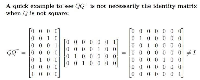
Current
Note has been deleted
Field-by-field Comparison
| Field | Before | After |
|---|---|---|
| Text | ||
| Extra |
Note 1216: ETH::1. Semester::LinAlg
Deck: ETH::1. Semester::LinAlg
Note Type: Horvath Cloze
GUID:
deleted
Note Type: Horvath Cloze
GUID:
Ep]9V3~H?2
Deleted Note
Front
Let \(A \in \mathbb{R}^{m \times n}\). Then \(C(A^\top) = C(A^\top A)\). Proof Included
Back
Let \(A \in \mathbb{R}^{m \times n}\). Then \(C(A^\top) = C(A^\top A)\). Proof Included
\(C(A^\top) = C(A^\top A)\) holds because:
- if \(x \in C(A^\top A)\) then let \(\exists y \ A^\top Ay = x\) and if we set \(z = Ay\) then \(A^\top z = x\) thus \(x \in C(A^\top)\).
- \(C(A^\top) = N(A)^\bot = N(A^\top A )^\bot\) as (\(N(A^\top A) = N(A)\)).
Then \(N(A^\top A)^\bot = C((A^\top A)^\top)\) (by \(N(B)^\bot = C(B^\top)\))
and \((A^\top A)^\top = A^\top A\) thus \(C(A^\top) = C(A^\top A)\).
Current
Note has been deleted
Field-by-field Comparison
| Field | Before | After |
|---|---|---|
| Text | ||
| Extra |
Note 1217: ETH::1. Semester::LinAlg
Deck: ETH::1. Semester::LinAlg
Note Type: Horvath Cloze
GUID:
deleted
Note Type: Horvath Cloze
GUID:
Eq^?6E3]XJ
Deleted Note
Front
The rank of a real symmetric matrix \(A\) is the number of non-zero eigenvalues (counting repetitions).
Back
The rank of a real symmetric matrix \(A\) is the number of non-zero eigenvalues (counting repetitions).
Current
Note has been deleted
Field-by-field Comparison
| Field | Before | After |
|---|---|---|
| Text |
Note 1218: ETH::1. Semester::LinAlg
Deck: ETH::1. Semester::LinAlg
Note Type: Horvath Cloze
GUID:
deleted
Note Type: Horvath Cloze
GUID:
F@!OqZ7#Kb
Deleted Note
Front
For Least Squares, \(A\) needs to have linearly independent columns which they are if \(t_i = t_j\) for all \(i \not = j\) .
This is guaranteed if all datapoints are unique in time.
This is guaranteed if all datapoints are unique in time.
Back
For Least Squares, \(A\) needs to have linearly independent columns which they are if \(t_i = t_j\) for all \(i \not = j\) .
This is guaranteed if all datapoints are unique in time.
This is guaranteed if all datapoints are unique in time.
Otherwise the projection is not defined, i.e. there's no unique solution to the normal equations.
Current
Note has been deleted
Field-by-field Comparison
| Field | Before | After |
|---|---|---|
| Text | ||
| Extra |
Note 1219: ETH::1. Semester::LinAlg
Deck: ETH::1. Semester::LinAlg
Note Type: Horvath Cloze
GUID:
deleted
Note Type: Horvath Cloze
GUID:
FAD$sgwJY?
Deleted Note
Front
Let \(A \in \mathbb{R}^{n \times n}\). If \((\lambda, v)\) is an eigenvalue, eigenvector pair, then {{c1::\((\overline{\lambda}, \overline{v})\) }} is an eigenvalue, eigenvector pair.
Back
Let \(A \in \mathbb{R}^{n \times n}\). If \((\lambda, v)\) is an eigenvalue, eigenvector pair, then {{c1::\((\overline{\lambda}, \overline{v})\) }} is an eigenvalue, eigenvector pair.
The conjugate is always also an EW, EV pair.
Current
Note has been deleted
Field-by-field Comparison
| Field | Before | After |
|---|---|---|
| Text | ||
| Extra |
Note 1220: ETH::1. Semester::LinAlg
Deck: ETH::1. Semester::LinAlg
Note Type: Horvath Cloze
GUID:
deleted
Note Type: Horvath Cloze
GUID:
FTH7rOs5Fz
Deleted Note
Front
Every polynomial \(P(z) = a_n z^n + a_{n - 1} z^{n - 1} + \dots + a_1 z + a_0\) with \(a_n \neq 0\) has {{c1:: a zero \(\lambda \in \mathbb{C} \)}}.
Back
Every polynomial \(P(z) = a_n z^n + a_{n - 1} z^{n - 1} + \dots + a_1 z + a_0\) with \(a_n \neq 0\) has {{c1:: a zero \(\lambda \in \mathbb{C} \)}}.
Fundamental theorem of algebra
Current
Note has been deleted
Field-by-field Comparison
| Field | Before | After |
|---|---|---|
| Text | ||
| Extra |
Note 1221: ETH::1. Semester::LinAlg
Deck: ETH::1. Semester::LinAlg
Note Type: Horvath Classic
GUID:
deleted
Note Type: Horvath Classic
GUID:
FX{E
Deleted Note
Front
SVD from rank 1 matrices with \(\sigma_1, \dots, \sigma_r\) be the non-zero singular values of \(A\), \(u_1, \dots, u_r\) the corresponding left singular vectors and \(v_1, \dots, v_r\) the corresponding right singular vectors.
Back
SVD from rank 1 matrices with \(\sigma_1, \dots, \sigma_r\) be the non-zero singular values of \(A\), \(u_1, \dots, u_r\) the corresponding left singular vectors and \(v_1, \dots, v_r\) the corresponding right singular vectors.
We have:\[ A = \sum_{k = 1}^r \sigma_k u_k v_k^\top \]
This follows directly from the compact SVD:
\[A = U_r \Sigma_r V_r^T = \begin{bmatrix} | & & | \\ \mathbf{u}_1 & \cdots & \mathbf{u}_r \\ | & & | \end{bmatrix} \begin{bmatrix} \sigma_1 & & \\ & \ddots & \\ & & \sigma_r \end{bmatrix} \begin{bmatrix} - & \mathbf{v}_1^T & - \\ & \vdots & \\ - & \mathbf{v}_r^T & - \end{bmatrix}\]
Expanding the matrix multiplication, we get:
\[A = \sigma_1 \mathbf{u}_1 \mathbf{v}_1^T + \sigma_2 \mathbf{u}_2 \mathbf{v}_2^T + \dots + \sigma_r \mathbf{u}_r \mathbf{v}_r^T = \sum_{i=1}^r \sigma_i \mathbf{u}_i \mathbf{v}_i^T\]
Each term \(\sigma_i \mathbf{u}_i \mathbf{v}_i^T\) is a rank-1 matrix because it is the outer product of two vectors, \(\mathbf{u}_i\) and \(\mathbf{v}_i\), scaled by the singular value \(\sigma_i\).
Current
Note has been deleted
Field-by-field Comparison
| Field | Before | After |
|---|---|---|
| Front | ||
| Back |
Note 1222: ETH::1. Semester::LinAlg
Deck: ETH::1. Semester::LinAlg
Note Type: Horvath Cloze
GUID:
deleted
Note Type: Horvath Cloze
GUID:
F]H_)uK%+@
Deleted Note
Front
Express the Fibonacci formula \(f_n = f_{n - 1} + f_{n - 2}\) as a matrix equation?
- {{c1::Let \(\mathbf{g}_{n+1} = M\mathbf{g}_n\), where \(M = \begin{bmatrix} 1 & 1 \\ 1 & 0 \end{bmatrix} \)(matrix version of the recursion)}}
- {{c2::The eigenvalues \(\lambda_1 = \frac{1+\sqrt{5} }{2}\) (golden ratio \(\phi\)) and \(\lambda_2 = \frac{1-\sqrt{5} }{2}\) are found, along with their eigenvectors \(v_1 = \begin{pmatrix} \lambda_1 \\ 1 \end{pmatrix}\) and \(v_2 = \begin{pmatrix} \lambda_2 \\ 1 \end{pmatrix}\) . These eigenvectors are independent since \(\lambda_1 \neq \lambda_2\) and thus they form a basis for \(\mathbb{R}^2\).}}
- {{c3::The initial state \(\mathbf{g}_0\) is written as a linear combination of eigenvectors with coefficients \(\pm\frac{1}{\sqrt{5} }\): \(g_0 = \frac{1}{\sqrt{5} }v_1 - \frac{1}{\sqrt{5} }v_2\).}}
- {{c4::Since \(M^n\mathbf{v}_i = \lambda_i^n\mathbf{v}_i\), we get the closed form: \[F_n = \frac{1}{\sqrt{5} } \left[\left(\frac{1+\sqrt{5} } {2}\right)^n - \left(\frac{1-\sqrt{5} } {2}\right)^n\right] \] }}
Back
Express the Fibonacci formula \(f_n = f_{n - 1} + f_{n - 2}\) as a matrix equation?
- {{c1::Let \(\mathbf{g}_{n+1} = M\mathbf{g}_n\), where \(M = \begin{bmatrix} 1 & 1 \\ 1 & 0 \end{bmatrix} \)(matrix version of the recursion)}}
- {{c2::The eigenvalues \(\lambda_1 = \frac{1+\sqrt{5} }{2}\) (golden ratio \(\phi\)) and \(\lambda_2 = \frac{1-\sqrt{5} }{2}\) are found, along with their eigenvectors \(v_1 = \begin{pmatrix} \lambda_1 \\ 1 \end{pmatrix}\) and \(v_2 = \begin{pmatrix} \lambda_2 \\ 1 \end{pmatrix}\) . These eigenvectors are independent since \(\lambda_1 \neq \lambda_2\) and thus they form a basis for \(\mathbb{R}^2\).}}
- {{c3::The initial state \(\mathbf{g}_0\) is written as a linear combination of eigenvectors with coefficients \(\pm\frac{1}{\sqrt{5} }\): \(g_0 = \frac{1}{\sqrt{5} }v_1 - \frac{1}{\sqrt{5} }v_2\).}}
- {{c4::Since \(M^n\mathbf{v}_i = \lambda_i^n\mathbf{v}_i\), we get the closed form: \[F_n = \frac{1}{\sqrt{5} } \left[\left(\frac{1+\sqrt{5} } {2}\right)^n - \left(\frac{1-\sqrt{5} } {2}\right)^n\right] \] }}
Current
Note has been deleted
Field-by-field Comparison
| Field | Before | After |
|---|---|---|
| Text |
Note 1223: ETH::1. Semester::LinAlg
Deck: ETH::1. Semester::LinAlg
Note Type: Horvath Cloze
GUID:
deleted
Note Type: Horvath Cloze
GUID:
Fb-7Ek~j3;
Deleted Note
Front
The eigenvalues of \(A^{-1}\) are \(1/\lambda_i\) if \(\lambda_i\)'s are the eigenvalues of \(A\).
Back
The eigenvalues of \(A^{-1}\) are \(1/\lambda_i\) if \(\lambda_i\)'s are the eigenvalues of \(A\).
Current
Note has been deleted
Field-by-field Comparison
| Field | Before | After |
|---|---|---|
| Text |
Note 1224: ETH::1. Semester::LinAlg
Deck: ETH::1. Semester::LinAlg
Note Type: Horvath Cloze
GUID:
deleted
Note Type: Horvath Cloze
GUID:
Fdf#%+wdU#
Deleted Note
Front
In the SVD the diagonal elements of \(\Sigma\), \(\sigma_i = \Sigma_{ii}\) are called the singular values of \(A\) and are {{c1:: ordered as \(\sigma_1 \geq \dots \sigma_{\min\{m, n\} }\)}}.
Back
In the SVD the diagonal elements of \(\Sigma\), \(\sigma_i = \Sigma_{ii}\) are called the singular values of \(A\) and are {{c1:: ordered as \(\sigma_1 \geq \dots \sigma_{\min\{m, n\} }\)}}.
Current
Note has been deleted
Field-by-field Comparison
| Field | Before | After |
|---|---|---|
| Text |
Note 1225: ETH::1. Semester::LinAlg
Deck: ETH::1. Semester::LinAlg
Note Type: Horvath Cloze
GUID:
deleted
Note Type: Horvath Cloze
GUID:
FjSbP7PsTQ
Deleted Note
Front
\(A^\dagger A\) is the projection matrix onto \(C(A^\top)\).
Back
\(A^\dagger A\) is the projection matrix onto \(C(A^\top)\).
Current
Note has been deleted
Field-by-field Comparison
| Field | Before | After |
|---|---|---|
| Text |
Note 1226: ETH::1. Semester::LinAlg
Deck: ETH::1. Semester::LinAlg
Note Type: Horvath Cloze
GUID:
deleted
Note Type: Horvath Cloze
GUID:
Fp:$8m1l7(
Deleted Note
Front
A vector space \(V\) is called finitely generated if {{c2::there exists a finite subset \(G \subseteq V\) with \(\textbf{Span}(G) = V\)}}.
Back
A vector space \(V\) is called finitely generated if {{c2::there exists a finite subset \(G \subseteq V\) with \(\textbf{Span}(G) = V\)}}.
Current
Note has been deleted
Field-by-field Comparison
| Field | Before | After |
|---|---|---|
| Text |
Note 1227: ETH::1. Semester::LinAlg
Deck: ETH::1. Semester::LinAlg
Note Type: Horvath Cloze
GUID:
deleted
Note Type: Horvath Cloze
GUID:
F{P9Py-@Ws
Deleted Note
Front
The singular values are the square-root of the eigenvalues of \(A^\top A\) (or \(AA^\top\)). Proof Included
Back
The singular values are the square-root of the eigenvalues of \(A^\top A\) (or \(AA^\top\)). Proof Included
Note that \(A^\top A\) and \(AA^\top\) share all non-zero eigenvalues. This can be seen easily as \(A^\top A\) is symmetric thus \(A^\top A = V^\top \Lambda V V(\Sigma^\top \Sigma) V^\top\) which implies that \(\Lambda = \Sigma^\top \Sigma\) and thus \(\lambda_i = \sigma_i^2\).
Current
Note has been deleted
Field-by-field Comparison
| Field | Before | After |
|---|---|---|
| Text | ||
| Extra |
Note 1228: ETH::1. Semester::LinAlg
Deck: ETH::1. Semester::LinAlg
Note Type: Horvath Cloze
GUID:
deleted
Note Type: Horvath Cloze
GUID:
F~GapB(@u;
Deleted Note
Front
If \(A \in \mathbb{R}^{m \times n}\) has rank \(r = m\), then \(Ax = b\) has a solution for {{c1::every \(b \in \mathbb{R}^m\) (equivalent to saying that \(\textbf{C}(A) = \mathbb{R}^m\))}}.
We call \(A\) solvable (invertible \(A\) is a special case of this).
We call \(A\) solvable (invertible \(A\) is a special case of this).
Back
If \(A \in \mathbb{R}^{m \times n}\) has rank \(r = m\), then \(Ax = b\) has a solution for {{c1::every \(b \in \mathbb{R}^m\) (equivalent to saying that \(\textbf{C}(A) = \mathbb{R}^m\))}}.
We call \(A\) solvable (invertible \(A\) is a special case of this).
We call \(A\) solvable (invertible \(A\) is a special case of this).
Current
Note has been deleted
Field-by-field Comparison
| Field | Before | After |
|---|---|---|
| Text |
Note 1229: ETH::1. Semester::LinAlg
Deck: ETH::1. Semester::LinAlg
Note Type: Horvath Classic
GUID:
deleted
Note Type: Horvath Classic
GUID:
G(7.sQ=i_?
Deleted Note
Front
Proof that the Rayleigh Quotient has it's maximum and minimum at the largest/smallest EWs?
Back
Proof that the Rayleigh Quotient has it's maximum and minimum at the largest/smallest EWs?
It is easy to see that \(R(v_{\max}) = \lambda_{\max}\) and \(R(v_{\min}) = \lambda_{\min}\).
See:
\(R(v_{\text{max}}) = \frac{v_{\text{max}}^\top A v_{\text{max}}}{v_{\text{max}}^\top v_{\text{max}}} = \frac{v_{\text{max}}^\top (\lambda_{\text{max}} v_{\text{max}})}{v_{\text{max}}^\top v_{\text{max}}} = \lambda_{\text{max}}\)
Current
Note has been deleted
Field-by-field Comparison
| Field | Before | After |
|---|---|---|
| Front | ||
| Back |
Note 1230: ETH::1. Semester::LinAlg
Deck: ETH::1. Semester::LinAlg
Note Type: Horvath Cloze
GUID:
deleted
Note Type: Horvath Cloze
GUID:
G1|bG=ffVu
Deleted Note
Front
Let \(Q\) be the \(m \times n\) matrix whose columns are an orthonormal basis of \(C(A)\).
Then the projection matrix that projects to \(C(A)\) is given by \(QQ^\top\). Proof Included
Back
Let \(Q\) be the \(m \times n\) matrix whose columns are an orthonormal basis of \(C(A)\).
Then the projection matrix that projects to \(C(A)\) is given by \(QQ^\top\). Proof Included
\(Q^\top Q\) simplifies to \(I\) in the case where our \(Q\) is orthogonal.
Thus \(P = Q (Q^\top Q)^{-1} Q^\top\) simplifies to \(P = QQ^\top\).
Thus \(P = Q (Q^\top Q)^{-1} Q^\top\) simplifies to \(P = QQ^\top\).
Current
Note has been deleted
Field-by-field Comparison
| Field | Before | After |
|---|---|---|
| Text | ||
| Extra |
Note 1231: ETH::1. Semester::LinAlg
Deck: ETH::1. Semester::LinAlg
Note Type: Horvath Classic
GUID:
deleted
Note Type: Horvath Classic
GUID:
G2Hf{n(RiQ
Deleted Note
Front
How do we get the \(QR\) decomposition for \(A\) with linearly independent columns?
Back
How do we get the \(QR\) decomposition for \(A\) with linearly independent columns?
- \(Q\) is the result of Gram-Schmidt on \(A\)
- \(R = Q^\top A\)
Current
Note has been deleted
Field-by-field Comparison
| Field | Before | After |
|---|---|---|
| Front | ||
| Back |
Note 1232: ETH::1. Semester::LinAlg
Deck: ETH::1. Semester::LinAlg
Note Type: Horvath Cloze
GUID:
deleted
Note Type: Horvath Cloze
GUID:
G9![k&wZRU
Deleted Note
Front
Given a symmetric matrix \(A \in \mathbb{R}^{n \times n}\) the Rayleigh Quotient defined for \(x \in \mathbb{R}^n \setminus {0}\), as \[ R(x) = {{c1::\frac{x^\top Ax}{x^\top x} }}\]attains it’s
- maximum at {{c2::\(R(v_{\text{max} }) = \lambda_{\text{max} }\)}}
- minimum at {{c2::\(R(v_{\text{min} }) = \lambda_{\text{min} } \)}}
where {{c2::\(\lambda_{\text{max} }\) and \(\lambda_{\text{min} }\) are respectively the largest and smallest eigenvalues of \(A\) and \(v_{\text{max} }\) and \(v_{\text{min} }\) their associated eigenvectors}}.
Back
Given a symmetric matrix \(A \in \mathbb{R}^{n \times n}\) the Rayleigh Quotient defined for \(x \in \mathbb{R}^n \setminus {0}\), as \[ R(x) = {{c1::\frac{x^\top Ax}{x^\top x} }}\]attains it’s
- maximum at {{c2::\(R(v_{\text{max} }) = \lambda_{\text{max} }\)}}
- minimum at {{c2::\(R(v_{\text{min} }) = \lambda_{\text{min} } \)}}
where {{c2::\(\lambda_{\text{max} }\) and \(\lambda_{\text{min} }\) are respectively the largest and smallest eigenvalues of \(A\) and \(v_{\text{max} }\) and \(v_{\text{min} }\) their associated eigenvectors}}.
Current
Note has been deleted
Field-by-field Comparison
| Field | Before | After |
|---|---|---|
| Text |
Note 1233: ETH::1. Semester::LinAlg
Deck: ETH::1. Semester::LinAlg
Note Type: Horvath Cloze
GUID:
deleted
Note Type: Horvath Cloze
GUID:
G^)Gmk^Z%6
Deleted Note
Front
Every matrix \(A \in \mathbb{R}^{m \times n}\) has an SVD decomposition. In other words:
Every linear transformation is diagonal when viewed in the bases of the singular vectors.
Back
Every matrix \(A \in \mathbb{R}^{m \times n}\) has an SVD decomposition. In other words:
Every linear transformation is diagonal when viewed in the bases of the singular vectors.
Current
Note has been deleted
Field-by-field Comparison
| Field | Before | After |
|---|---|---|
| Text |
Note 1234: ETH::1. Semester::LinAlg
Deck: ETH::1. Semester::LinAlg
Note Type: Horvath Classic
GUID:
deleted
Note Type: Horvath Classic
GUID:
Gp{ARt+OX,
Deleted Note
Front
If you have some expression \(x_1 + i x_2 = y_1 + i y_2\) we can separate this into?
Back
If you have some expression \(x_1 + i x_2 = y_1 + i y_2\) we can separate this into?
- \(x_1 = y_1\)
- \(x_2 = y_2\)
Current
Note has been deleted
Field-by-field Comparison
| Field | Before | After |
|---|---|---|
| Front | ||
| Back |
Note 1235: ETH::1. Semester::LinAlg
Deck: ETH::1. Semester::LinAlg
Note Type: Horvath Classic
GUID:
deleted
Note Type: Horvath Classic
GUID:
HM?p0`y8nB
Deleted Note
Front
A matrix \(R\) is in RREF if:
Back
A matrix \(R\) is in RREF if:
- For every \(i \in [r]\), column \(j_i\) of \(R\) is the standard unit vector \(e_i\)
- All entries \(r_{ij}\) “below the staircase” are \(0\).
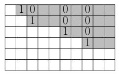
Current
Note has been deleted
Field-by-field Comparison
| Field | Before | After |
|---|---|---|
| Front | ||
| Back |
Note 1236: ETH::1. Semester::LinAlg
Deck: ETH::1. Semester::LinAlg
Note Type: Horvath Classic
GUID:
deleted
Note Type: Horvath Classic
GUID:
HO&p/zi-tL
Deleted Note
Front
How is the scalar product defined on an angle?
Back
How is the scalar product defined on an angle?
\(\textbf{v} \cdot \textbf{w} = ||\textbf{v}|| \ ||\textbf{w}|| \cdot \cos(\alpha)\).
If v and w are unit vectors, we don't need to divide by their norms, see the definition of a scalar product geometrically.
If v and w are unit vectors, we don't need to divide by their norms, see the definition of a scalar product geometrically.
Current
Note has been deleted
Field-by-field Comparison
| Field | Before | After |
|---|---|---|
| Front | ||
| Back |
Note 1237: ETH::1. Semester::LinAlg
Deck: ETH::1. Semester::LinAlg
Note Type: Horvath Cloze
GUID:
deleted
Note Type: Horvath Cloze
GUID:
HVb7^Pa98H
Deleted Note
Front
All eigenvalues are exactly the roots of the polynomial \(\det(A - \lambda I)\).
Back
All eigenvalues are exactly the roots of the polynomial \(\det(A - \lambda I)\).
Current
Note has been deleted
Field-by-field Comparison
| Field | Before | After |
|---|---|---|
| Text |
Note 1238: ETH::1. Semester::LinAlg
Deck: ETH::1. Semester::LinAlg
Note Type: Horvath Classic
GUID:
deleted
Note Type: Horvath Classic
GUID:
Hept`QKpE8
Deleted Note
Front
What is the Kronecker delta?
Back
What is the Kronecker delta?
A function which is described as follows:
\(\delta_{i, j} = \begin{cases} \text{0} &\quad\text{if }i \neq j \\ \text{1} &\quad\text{if }i = j \end{cases}\)
\(\delta_{i, j} = \begin{cases} \text{0} &\quad\text{if }i \neq j \\ \text{1} &\quad\text{if }i = j \end{cases}\)
Current
Note has been deleted
Field-by-field Comparison
| Field | Before | After |
|---|---|---|
| Front | ||
| Back |
Note 1239: ETH::1. Semester::LinAlg
Deck: ETH::1. Semester::LinAlg
Note Type: Horvath Cloze
GUID:
deleted
Note Type: Horvath Cloze
GUID:
HgRNZ)7~Q=
Deleted Note
Front
Dimension of the nullspace \(\dim(N(A)) = \) {{c1:: \(n - r = n - \textbf{rank}(A)\)}}
Back
Dimension of the nullspace \(\dim(N(A)) = \) {{c1:: \(n - r = n - \textbf{rank}(A)\)}}
Current
Note has been deleted
Field-by-field Comparison
| Field | Before | After |
|---|---|---|
| Text |
Note 1240: ETH::1. Semester::LinAlg
Deck: ETH::1. Semester::LinAlg
Note Type: Horvath Cloze
GUID:
deleted
Note Type: Horvath Cloze
GUID:
HnqZA9P|@G
Deleted Note
Front
Given a triangular (either upper or lower) matrix \(T \in \mathbb{R}^{n \times n}\), we have \[ \det(T) = {{c1:: \prod_{k = 1}^n T_{kk} }}\]
Back
Given a triangular (either upper or lower) matrix \(T \in \mathbb{R}^{n \times n}\), we have \[ \det(T) = {{c1:: \prod_{k = 1}^n T_{kk} }}\]
For a triangular matrix, if we choose an element off the diagonal, we are then forced to choose one in the \(0\)s thus making that factor \(0\). The only valid permutation is thus the \(\text{id}\), which means we just multiply the diagonals.
Current
Note has been deleted
Field-by-field Comparison
| Field | Before | After |
|---|---|---|
| Text | ||
| Extra |
Note 1241: ETH::1. Semester::LinAlg
Deck: ETH::1. Semester::LinAlg
Note Type: Horvath Cloze
GUID:
deleted
Note Type: Horvath Cloze
GUID:
I5WrW!E]G<
Deleted Note
Front
The determinant expressed in terms of co-factors is: \[\det(A) = {{c1:: \sum_{j = 1}^n A_{ij}C_{ij} }}\]
Back
The determinant expressed in terms of co-factors is: \[\det(A) = {{c1:: \sum_{j = 1}^n A_{ij}C_{ij} }}\]
in which we multiply the cofactor of every element by the element itself, as is clear in the example for a 3x3.
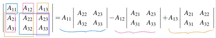
Current
Note has been deleted
Field-by-field Comparison
| Field | Before | After |
|---|---|---|
| Text | ||
| Extra |
Note 1242: ETH::1. Semester::LinAlg
Deck: ETH::1. Semester::LinAlg
Note Type: Horvath Classic
GUID:
deleted
Note Type: Horvath Classic
GUID:
ICEre
Deleted Note
Front
What does \(N(A) = \mathbb{R}^n\) mean?
Back
What does \(N(A) = \mathbb{R}^n\) mean?
it means \(A = \boldsymbol{0}\)
Current
Note has been deleted
Field-by-field Comparison
| Field | Before | After |
|---|---|---|
| Front | ||
| Back |
Note 1243: ETH::1. Semester::LinAlg
Deck: ETH::1. Semester::LinAlg
Note Type: Horvath Cloze
GUID:
deleted
Note Type: Horvath Cloze
GUID:
IX@x0?}8bL
Deleted Note
Front
\(A = \begin{bmatrix} 1 & 1 \\ 0 & 1 \end{bmatrix}\) is invertible but not diagonalisable since the EW \(1\) has algebraic multiplicity 2 but geometric multiplicity 1.
Back
\(A = \begin{bmatrix} 1 & 1 \\ 0 & 1 \end{bmatrix}\) is invertible but not diagonalisable since the EW \(1\) has algebraic multiplicity 2 but geometric multiplicity 1.
Current
Note has been deleted
Field-by-field Comparison
| Field | Before | After |
|---|---|---|
| Text |
Note 1244: ETH::1. Semester::LinAlg
Deck: ETH::1. Semester::LinAlg
Note Type: Horvath Cloze
GUID:
deleted
Note Type: Horvath Cloze
GUID:
I`-{jhD?WK
Deleted Note
Front
If \(Av = \lambda v\) and \(\lambda\) and \(v\) are an EW-EV pair we know \(v \neq 0\) .
Back
If \(Av = \lambda v\) and \(\lambda\) and \(v\) are an EW-EV pair we know \(v \neq 0\) .
Current
Note has been deleted
Field-by-field Comparison
| Field | Before | After |
|---|---|---|
| Text |
Note 1245: ETH::1. Semester::LinAlg
Deck: ETH::1. Semester::LinAlg
Note Type: Horvath Classic
GUID:
deleted
Note Type: Horvath Classic
GUID:
Ie1sVs`1ap
Deleted Note
Front
What is the inverse of \(A = \begin{bmatrix} a & b \\ c & d \end{bmatrix}\)?
Back
What is the inverse of \(A = \begin{bmatrix} a & b \\ c & d \end{bmatrix}\)?
\[A^{-1} = \frac{1}{ad - bc} \begin{bmatrix} d & -c \\ -b & a \end{bmatrix}\]
Current
Note has been deleted
Field-by-field Comparison
| Field | Before | After |
|---|---|---|
| Front | ||
| Back |
Note 1246: ETH::1. Semester::LinAlg
Deck: ETH::1. Semester::LinAlg
Note Type: Horvath Cloze
GUID:
deleted
Note Type: Horvath Cloze
GUID:
Ixx.9h)R+>
Deleted Note
Front
Give two examples of orthogonal matrices:
- 2x2 rotation matrices
- Permutation matrices
Back
Give two examples of orthogonal matrices:
- 2x2 rotation matrices
- Permutation matrices
Current
Note has been deleted
Field-by-field Comparison
| Field | Before | After |
|---|---|---|
| Text |
Note 1247: ETH::1. Semester::LinAlg
Deck: ETH::1. Semester::LinAlg
Note Type: Horvath Classic
GUID:
deleted
Note Type: Horvath Classic
GUID:
J,}qfri4M=
Deleted Note
Front
Was ist eine unitäre Matrix?
Back
Was ist eine unitäre Matrix?
Für eine unitäre Matrix gilt \( \mathbf{A^H A = I}_n\), d.h. die komplex-transponierte von A ist die Inverse von A.
Unitär = regulär & quadratisch
Current
Note has been deleted
Field-by-field Comparison
| Field | Before | After |
|---|---|---|
| Front | ||
| Back |
Note 1248: ETH::1. Semester::LinAlg
Deck: ETH::1. Semester::LinAlg
Note Type: Horvath Cloze
GUID:
deleted
Note Type: Horvath Cloze
GUID:
J0-A1[(zwf
Deleted Note
Front
We know that \(\forall x \in \mathbb{R}^n\), there exist \(x_0 \in N(A)\) and \(x_1 \in R(A)\) such that \(x = x_0 + x_1 \) and \(x_1^\top x_0 = 0\) as \(N(A) = C(A^\top)^\perp\) are orthogonal complements.
Back
We know that \(\forall x \in \mathbb{R}^n\), there exist \(x_0 \in N(A)\) and \(x_1 \in R(A)\) such that \(x = x_0 + x_1 \) and \(x_1^\top x_0 = 0\) as \(N(A) = C(A^\top)^\perp\) are orthogonal complements.
Current
Note has been deleted
Field-by-field Comparison
| Field | Before | After |
|---|---|---|
| Text |
Note 1249: ETH::1. Semester::LinAlg
Deck: ETH::1. Semester::LinAlg
Note Type: Horvath Classic
GUID:
deleted
Note Type: Horvath Classic
GUID:
J1MYsJ:|-Q
Deleted Note
Front
An linear combination of \(\lambda_1\textbf{v}_1 + \lambda_2\textbf{v}_2 + \dots + \lambda_n\textbf{v}_n\) is convex if
Back
An linear combination of \(\lambda_1\textbf{v}_1 + \lambda_2\textbf{v}_2 + \dots + \lambda_n\textbf{v}_n\) is convex if
it is both affine and conic
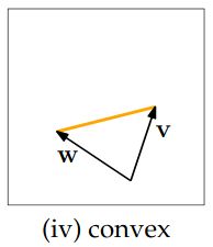
Current
Note has been deleted
Field-by-field Comparison
| Field | Before | After |
|---|---|---|
| Front | ||
| Back |
Note 1250: ETH::1. Semester::LinAlg
Deck: ETH::1. Semester::LinAlg
Note Type: Horvath Classic
GUID:
deleted
Note Type: Horvath Classic
GUID:
J<060JA%BR
Deleted Note
Front
Can a nilpotent matrix have an inverse?
Back
Can a nilpotent matrix have an inverse?
No, as the \(0\) matrix does not have an inverse.
Current
Note has been deleted
Field-by-field Comparison
| Field | Before | After |
|---|---|---|
| Front | ||
| Back |
Note 1251: ETH::1. Semester::LinAlg
Deck: ETH::1. Semester::LinAlg
Note Type: Horvath Classic
GUID:
deleted
Note Type: Horvath Classic
GUID:
JAn~&+e&|!
Deleted Note
Front
The determinant is linear in each row (or each column). In other words for any \(a_0, a_1, a_2, \dots, a_n \in \mathbb{R}^n\) and \(\alpha_0, \alpha_1 \in \mathbb{R}\) we have: (Two linearity properties)
Back
The determinant is linear in each row (or each column). In other words for any \(a_0, a_1, a_2, \dots, a_n \in \mathbb{R}^n\) and \(\alpha_0, \alpha_1 \in \mathbb{R}\) we have: (Two linearity properties)
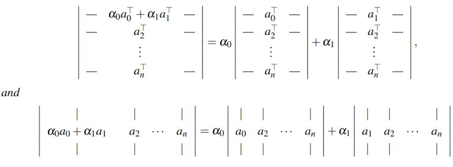
Current
Note has been deleted
Field-by-field Comparison
| Field | Before | After |
|---|---|---|
| Front | ||
| Back |
Note 1252: ETH::1. Semester::LinAlg
Deck: ETH::1. Semester::LinAlg
Note Type: Horvath Cloze
GUID:
deleted
Note Type: Horvath Cloze
GUID:
JG.Pzp,r%b
Deleted Note
Front
Wenn \(A,B\) invertierbar sind, dann ist es {{c1::\((AB)^{-1}=B^{-1}A^{-1}\)}} auch.
Back
Wenn \(A,B\) invertierbar sind, dann ist es {{c1::\((AB)^{-1}=B^{-1}A^{-1}\)}} auch.
Current
Note has been deleted
Field-by-field Comparison
| Field | Before | After |
|---|---|---|
| Text |
Note 1253: ETH::1. Semester::LinAlg
Deck: ETH::1. Semester::LinAlg
Note Type: Horvath Classic
GUID:
deleted
Note Type: Horvath Classic
GUID:
JIi?26WP]C
Deleted Note
Front
What is the triangle inequality?
Back
What is the triangle inequality?

This follows from the geometric interpretation in two dimensions, generalised.
Current
Note has been deleted
Field-by-field Comparison
| Field | Before | After |
|---|---|---|
| Front | ||
| Back |
Note 1254: ETH::1. Semester::LinAlg
Deck: ETH::1. Semester::LinAlg
Note Type: Horvath Classic
GUID:
deleted
Note Type: Horvath Classic
GUID:
JlD}ITLxEy
Deleted Note
Front
What is the composition of two linear transformations \(T_A \circ T_B\)?
Back
What is the composition of two linear transformations \(T_A \circ T_B\)?
\(T_A \circ T_B = T_{AB}\)
Current
Note has been deleted
Field-by-field Comparison
| Field | Before | After |
|---|---|---|
| Front | ||
| Back |
Note 1255: ETH::1. Semester::LinAlg
Deck: ETH::1. Semester::LinAlg
Note Type: Horvath Cloze
GUID:
deleted
Note Type: Horvath Cloze
GUID:
JmsF:FMC~D
Deleted Note
Front
Let \(V\) and \(W\) be orthogonal subspaces.
Then \(V \cap W = \) {{c1:: \(\{0\}\) (as all subspaces contain the \(0\) vector)}}.
Back
Let \(V\) and \(W\) be orthogonal subspaces.
Then \(V \cap W = \) {{c1:: \(\{0\}\) (as all subspaces contain the \(0\) vector)}}.
Current
Note has been deleted
Field-by-field Comparison
| Field | Before | After |
|---|---|---|
| Text |
Note 1256: ETH::1. Semester::LinAlg
Deck: ETH::1. Semester::LinAlg
Note Type: Horvath Cloze
GUID:
deleted
Note Type: Horvath Cloze
GUID:
K-XRXZqOV,
Deleted Note
Front
If \(AB = BA\), then \(A,B\) share an EV.
Back
If \(AB = BA\), then \(A,B\) share an EV.
Assume \(AB = BA\).
If \(\lambda, v\) an EW-EV pair of \(A\) then \(A(Bv) = (AB)v = B(Av) = \lambda Bv\) thus \(Bv\) is an eigenvector of \(A\).
Then \(Bv\) is a multiple of some \(v\) of that EW \(\lambda\) (easiest to see for \(A\) complete set of real EVs) \(\implies\) \(Bv = \lambda'v\) thus that \(v\) is also an EV of \(B\).
Current
Note has been deleted
Field-by-field Comparison
| Field | Before | After |
|---|---|---|
| Text | ||
| Extra |
Note 1257: ETH::1. Semester::LinAlg
Deck: ETH::1. Semester::LinAlg
Note Type: Horvath Cloze
GUID:
deleted
Note Type: Horvath Cloze
GUID:
K4@L>.#ir<
Deleted Note
Front
For all matrices \(A\):
\((A^\top)^\top = \)\(A\)
\((A^\top)^\top = \)\(A\)
Back
For all matrices \(A\):
\((A^\top)^\top = \)\(A\)
\((A^\top)^\top = \)\(A\)
Current
Note has been deleted
Field-by-field Comparison
| Field | Before | After |
|---|---|---|
| Text |
Note 1258: ETH::1. Semester::LinAlg
Deck: ETH::1. Semester::LinAlg
Note Type: Horvath Cloze
GUID:
deleted
Note Type: Horvath Cloze
GUID:
K9{>JhFX!.
Deleted Note
Front
\((A^\top)^\dagger = (A^\dagger)^\top \)
Back
\((A^\top)^\dagger = (A^\dagger)^\top \)
Current
Note has been deleted
Field-by-field Comparison
| Field | Before | After |
|---|---|---|
| Text |
Note 1259: ETH::1. Semester::LinAlg
Deck: ETH::1. Semester::LinAlg
Note Type: Horvath Cloze
GUID:
deleted
Note Type: Horvath Cloze
GUID:
K=a-HUOVwC
Deleted Note
Front
Three equivalent statements:
- {{c1::\(T_A : \mathbb{R}^m \rightarrow \mathbb{R}^m\) is bijective.::Transformation}}
- There is an \(m \times m\) matrix \(B\) such that \(BA = I\).
- The columns of \(A\) are linearly independent.
Back
Three equivalent statements:
- {{c1::\(T_A : \mathbb{R}^m \rightarrow \mathbb{R}^m\) is bijective.::Transformation}}
- There is an \(m \times m\) matrix \(B\) such that \(BA = I\).
- The columns of \(A\) are linearly independent.
The third one can be derived from the fact that if \(BA = I\), there is only a single \(x \in \mathbb{R}^m\) such that \(A \textbf{x} = 0\).
It is also intuitively clear that if not all columns were linearly independent, we'd actually have a tall linear transformation and would be losing information.
It is also intuitively clear that if not all columns were linearly independent, we'd actually have a tall linear transformation and would be losing information.
Current
Note has been deleted
Field-by-field Comparison
| Field | Before | After |
|---|---|---|
| Text | ||
| Extra |
Note 1260: ETH::1. Semester::LinAlg
Deck: ETH::1. Semester::LinAlg
Note Type: Horvath Cloze
GUID:
deleted
Note Type: Horvath Cloze
GUID:
KAa7x3sA#0
Deleted Note
Front
The eigenvalues of \(A + B\) are not correlated.
Back
The eigenvalues of \(A + B\) are not correlated.
Current
Note has been deleted
Field-by-field Comparison
| Field | Before | After |
|---|---|---|
| Text |
Note 1261: ETH::1. Semester::LinAlg
Deck: ETH::1. Semester::LinAlg
Note Type: Horvath Cloze
GUID:
deleted
Note Type: Horvath Cloze
GUID:
KUMMEUP]kH
Deleted Note
Front
In a vector space \(V\) three important properties hold:
- \(0v = 0\) for all \(v\)
- there is only one \(0\)
- one unique inverse \(-v\) for all \(v\)
Back
In a vector space \(V\) three important properties hold:
- \(0v = 0\) for all \(v\)
- there is only one \(0\)
- one unique inverse \(-v\) for all \(v\)
Current
Note has been deleted
Field-by-field Comparison
| Field | Before | After |
|---|---|---|
| Text |
Note 1262: ETH::1. Semester::LinAlg
Deck: ETH::1. Semester::LinAlg
Note Type: Horvath Classic
GUID:
deleted
Note Type: Horvath Classic
GUID:
KW-&%*&l;g
Deleted Note
Front
Was ist eine reguläre Matrix?
Back
Was ist eine reguläre Matrix?
Eine Matrix \( A \) mit \(\text{Rang}(A) = n\).
regulär \( \iff \) invertierbar
Current
Note has been deleted
Field-by-field Comparison
| Field | Before | After |
|---|---|---|
| Front | ||
| Back |
Note 1263: ETH::1. Semester::LinAlg
Deck: ETH::1. Semester::LinAlg
Note Type: Horvath Classic
GUID:
deleted
Note Type: Horvath Classic
GUID:
KZs-,vID&:
Deleted Note
Front
What are kernel and image of a linear transformation?
Back
What are kernel and image of a linear transformation?
The kernel is the nullspace and the image the column space.
Current
Note has been deleted
Field-by-field Comparison
| Field | Before | After |
|---|---|---|
| Front | ||
| Back |
Note 1264: ETH::1. Semester::LinAlg
Deck: ETH::1. Semester::LinAlg
Note Type: Horvath Classic
GUID:
deleted
Note Type: Horvath Classic
GUID:
KvqIdKEm_e
Deleted Note
Front
What happens if \(A\) itself is invertible for the projection matrix?
Back
What happens if \(A\) itself is invertible for the projection matrix?
Since \(A\) is invertible, it spans \(\mathbb{R}^m\) and any projection is simply the point itself.
This is beautifully reflected in the fact that if we simplify \(P = A A^{-1} (A^\top)^{-1} A^\top\) then we simply get \(P = I\).
In general it may look like we can simplify the expression for the projection matrix \(P\), this is however not the case, UNLESS \(A\) is invertible:
\((A^\top A)^{-1} = A^{-1} (A^\top)^{-1}\)
Current
Note has been deleted
Field-by-field Comparison
| Field | Before | After |
|---|---|---|
| Front | ||
| Back |
Note 1265: ETH::1. Semester::LinAlg
Deck: ETH::1. Semester::LinAlg
Note Type: Horvath Cloze
GUID:
deleted
Note Type: Horvath Cloze
GUID:
LEJ$Uw{FC{
Deleted Note
Front
Let \(A\) be an \(m \times n\) matrix and \(b \in \mathbb{R}^m\).
The set \[ \textbf{Sol}(A, b) := \{x \in \mathbb{R}^n : Ax = b\} \subseteq \mathbb{R}^n \] is the solution space of \(Ax = b\).
The set \[ \textbf{Sol}(A, b) := \{x \in \mathbb{R}^n : Ax = b\} \subseteq \mathbb{R}^n \] is the solution space of \(Ax = b\).
Back
Let \(A\) be an \(m \times n\) matrix and \(b \in \mathbb{R}^m\).
The set \[ \textbf{Sol}(A, b) := \{x \in \mathbb{R}^n : Ax = b\} \subseteq \mathbb{R}^n \] is the solution space of \(Ax = b\).
The set \[ \textbf{Sol}(A, b) := \{x \in \mathbb{R}^n : Ax = b\} \subseteq \mathbb{R}^n \] is the solution space of \(Ax = b\).
Current
Note has been deleted
Field-by-field Comparison
| Field | Before | After |
|---|---|---|
| Text |
Note 1266: ETH::1. Semester::LinAlg
Deck: ETH::1. Semester::LinAlg
Note Type: Horvath Cloze
GUID:
deleted
Note Type: Horvath Cloze
GUID:
LIjab7I=97
Deleted Note
Front
Let \(V\) be a vector space. A nonempty set \(U \subseteq V\) is called a subspace of \(V\) if the following two axioms of a subspace are true for all \(v, w \in U\) and all \(\lambda \in \mathbb{R}\):
- \(v + w \in U\) (closure addition)
- \(\lambda v \in U\) (closure multiplication)
Back
Let \(V\) be a vector space. A nonempty set \(U \subseteq V\) is called a subspace of \(V\) if the following two axioms of a subspace are true for all \(v, w \in U\) and all \(\lambda \in \mathbb{R}\):
- \(v + w \in U\) (closure addition)
- \(\lambda v \in U\) (closure multiplication)
Current
Note has been deleted
Field-by-field Comparison
| Field | Before | After |
|---|---|---|
| Text |
Note 1267: ETH::1. Semester::LinAlg
Deck: ETH::1. Semester::LinAlg
Note Type: Horvath Classic
GUID:
deleted
Note Type: Horvath Classic
GUID:
LR3$8)Rp9r
Deleted Note
Front
How can we make projections easier using orthogonality?
Back
How can we make projections easier using orthogonality?
We use Gram-Schmid to convert \(A\) into \(Q\) (the column spaces are equal).
We then project using \(QQ^\top\).
We then project using \(QQ^\top\).
Current
Note has been deleted
Field-by-field Comparison
| Field | Before | After |
|---|---|---|
| Front | ||
| Back |
Note 1268: ETH::1. Semester::LinAlg
Deck: ETH::1. Semester::LinAlg
Note Type: Horvath Cloze
GUID:
deleted
Note Type: Horvath Cloze
GUID:
LR~EpRNX@l
Deleted Note
Front
Intuition on the projection formula (in 2d):
- Assume \(\mathbf{a} \perp \mathbf{e}\) \(\implies\) \(\mathbf{a} \perp (\mathbf{b} - \mathbf{p})\) (define error vector \(\mathbf{e} = \mathbf{b} - \mathbf{p}\)).
- We can write \(\mathbf{p} = \lambda\mathbf{a}, \lambda \in \mathbb{R}\) since we know {{c1::the projection vector is on the line spanned by \(\mathbf{a}\) and hence \(\mathbf{p}\) is a scalar multiple of \(\textbf{a}\)}}.
- \[ \begin{align} \mathbf{a} \perp (\mathbf{b} - \mathbf{p}) &\iff {{c1:: \mathbf{a}^\top(\mathbf{b} - \mathbf{p}) = 0 \\ &\iff \mathbf{a}^\top(\mathbf{b} - \lambda\mathbf{a}) = 0 \\ &\iff \mathbf{a}^\top\mathbf{b} - \mathbf{a}^\top\lambda\mathbf{a} = 0 \\ &\iff \mathbf{a}^\top\mathbf{b} = \mathbf{a}^\top\lambda\mathbf{a} \\ &\iff \mathbf{a}^\top\mathbf{b} = \lambda\mathbf{a}^\top\mathbf{a} \\ &\iff \lambda = \frac{\mathbf{a}^\top\mathbf{b} }{\mathbf{a}^\top\mathbf{a} } }} \end{align} \]
- Where we first used \(\mathbf{v} \perp \mathbf{u} \iff \mathbf{v}^\top\mathbf{u} = 0\), then plugged in for \(\lambda a\) for \(p\), then used the distributivity of the vector multiplication.
- We can divide by \(a^\top a\)(\(a\) is a nonzero real number, as is a nonzero vector)
Back
Intuition on the projection formula (in 2d):
- Assume \(\mathbf{a} \perp \mathbf{e}\) \(\implies\) \(\mathbf{a} \perp (\mathbf{b} - \mathbf{p})\) (define error vector \(\mathbf{e} = \mathbf{b} - \mathbf{p}\)).
- We can write \(\mathbf{p} = \lambda\mathbf{a}, \lambda \in \mathbb{R}\) since we know {{c1::the projection vector is on the line spanned by \(\mathbf{a}\) and hence \(\mathbf{p}\) is a scalar multiple of \(\textbf{a}\)}}.
- \[ \begin{align} \mathbf{a} \perp (\mathbf{b} - \mathbf{p}) &\iff {{c1:: \mathbf{a}^\top(\mathbf{b} - \mathbf{p}) = 0 \\ &\iff \mathbf{a}^\top(\mathbf{b} - \lambda\mathbf{a}) = 0 \\ &\iff \mathbf{a}^\top\mathbf{b} - \mathbf{a}^\top\lambda\mathbf{a} = 0 \\ &\iff \mathbf{a}^\top\mathbf{b} = \mathbf{a}^\top\lambda\mathbf{a} \\ &\iff \mathbf{a}^\top\mathbf{b} = \lambda\mathbf{a}^\top\mathbf{a} \\ &\iff \lambda = \frac{\mathbf{a}^\top\mathbf{b} }{\mathbf{a}^\top\mathbf{a} } }} \end{align} \]
- Where we first used \(\mathbf{v} \perp \mathbf{u} \iff \mathbf{v}^\top\mathbf{u} = 0\), then plugged in for \(\lambda a\) for \(p\), then used the distributivity of the vector multiplication.
- We can divide by \(a^\top a\)(\(a\) is a nonzero real number, as is a nonzero vector)
Current
Note has been deleted
Field-by-field Comparison
| Field | Before | After |
|---|---|---|
| Text |
Note 1269: ETH::1. Semester::LinAlg
Deck: ETH::1. Semester::LinAlg
Note Type: Horvath Cloze
GUID:
deleted
Note Type: Horvath Cloze
GUID:
LXx2V/%q~V
Deleted Note
Front
For a system \(Ax = b\) Gauss-elimination fails only if \(A\) has linearly dependent columns.
Back
For a system \(Ax = b\) Gauss-elimination fails only if \(A\) has linearly dependent columns.
Current
Note has been deleted
Field-by-field Comparison
| Field | Before | After |
|---|---|---|
| Text |
Note 1270: ETH::1. Semester::LinAlg
Deck: ETH::1. Semester::LinAlg
Note Type: Horvath Cloze
GUID:
deleted
Note Type: Horvath Cloze
GUID:
LiA<-d|o$6
Deleted Note
Front
For all \(x\) and an orthogonal matrix \(Q\) we have \((Qx)^\top(Qy) = x^\top y\) Proof Included
Back
For all \(x\) and an orthogonal matrix \(Q\) we have \((Qx)^\top(Qy) = x^\top y\) Proof Included
\((Qx)^\top (Qy) = x^\top Q^\top Q y = x^\top I y = x^\top y\). since \(Q^\top Q = I\).
Current
Note has been deleted
Field-by-field Comparison
| Field | Before | After |
|---|---|---|
| Text | ||
| Extra |
Note 1271: ETH::1. Semester::LinAlg
Deck: ETH::1. Semester::LinAlg
Note Type: Horvath Classic
GUID:
deleted
Note Type: Horvath Classic
GUID:
Lr(&c[;1SI
Deleted Note
Front
A linear combination of \(\lambda_1\textbf{v}_1 + \lambda_2\textbf{v}_2 + \dots + \lambda_n\textbf{v}_n\) is conic if
Back
A linear combination of \(\lambda_1\textbf{v}_1 + \lambda_2\textbf{v}_2 + \dots + \lambda_n\textbf{v}_n\) is conic if
\(\lambda_j \geq 0\) for \(j = 1, 2, \dots, n\)
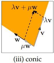
Current
Note has been deleted
Field-by-field Comparison
| Field | Before | After |
|---|---|---|
| Front | ||
| Back |
Note 1272: ETH::1. Semester::LinAlg
Deck: ETH::1. Semester::LinAlg
Note Type: Horvath Cloze
GUID:
deleted
Note Type: Horvath Cloze
GUID:
LvFIoMB!0)
Deleted Note
Front
By the spectral theorem, for any symmetric \(A\) we can write:
\[ A = V \Lambda V^\top \]where \(\Lambda \in \mathbb{R}^{n \times n}\) is a diagonal matrix with the eigenvalues of \(A\) in it's diagonal, and \(V\) orthogonal matrix containing the eigenvectors \(V^\top V = I\).
\[ A = V \Lambda V^\top \]where \(\Lambda \in \mathbb{R}^{n \times n}\) is a diagonal matrix with the eigenvalues of \(A\) in it's diagonal, and \(V\) orthogonal matrix containing the eigenvectors \(V^\top V = I\).
Back
By the spectral theorem, for any symmetric \(A\) we can write:
\[ A = V \Lambda V^\top \]where \(\Lambda \in \mathbb{R}^{n \times n}\) is a diagonal matrix with the eigenvalues of \(A\) in it's diagonal, and \(V\) orthogonal matrix containing the eigenvectors \(V^\top V = I\).
\[ A = V \Lambda V^\top \]where \(\Lambda \in \mathbb{R}^{n \times n}\) is a diagonal matrix with the eigenvalues of \(A\) in it's diagonal, and \(V\) orthogonal matrix containing the eigenvectors \(V^\top V = I\).
This decomposition is called an eigen-decomposition.
Current
Note has been deleted
Field-by-field Comparison
| Field | Before | After |
|---|---|---|
| Text | ||
| Extra |
Note 1273: ETH::1. Semester::LinAlg
Deck: ETH::1. Semester::LinAlg
Note Type: Horvath Cloze
GUID:
deleted
Note Type: Horvath Cloze
GUID:
Lxg{aBX]%>
Deleted Note
Front
Let \(\{v_1, \dots, v_m\}\) be a basis of \(V\). For each \(v \in V\), there are unique scalars \(\lambda_1, \dots, \lambda_n\) such that \[ v = \sum_{j = 1}^{m} \lambda_j v_j \]This means that in a basis each vector can be written as a unique linear combination.
Back
Let \(\{v_1, \dots, v_m\}\) be a basis of \(V\). For each \(v \in V\), there are unique scalars \(\lambda_1, \dots, \lambda_n\) such that \[ v = \sum_{j = 1}^{m} \lambda_j v_j \]This means that in a basis each vector can be written as a unique linear combination.
This holds as all basis vectors are linearly independent by definition.
Current
Note has been deleted
Field-by-field Comparison
| Field | Before | After |
|---|---|---|
| Text | ||
| Extra |
Note 1274: ETH::1. Semester::LinAlg
Deck: ETH::1. Semester::LinAlg
Note Type: Horvath Cloze
GUID:
deleted
Note Type: Horvath Cloze
GUID:
L|Y
Deleted Note
Front
Let \(A\) and \(v_1, \dots, v_k \in \mathbb{R}^n\) be the EVs of \(\lambda_1, \dots, \lambda_k \in \mathbb{R}^n\).
If the \(\lambda_1, \dots, \lambda_k\)s are all distinct then the EVs \(v_1, \dots, v_k\) are all linearly independent.
Back
Let \(A\) and \(v_1, \dots, v_k \in \mathbb{R}^n\) be the EVs of \(\lambda_1, \dots, \lambda_k \in \mathbb{R}^n\).
If the \(\lambda_1, \dots, \lambda_k\)s are all distinct then the EVs \(v_1, \dots, v_k\) are all linearly independent.
Current
Note has been deleted
Field-by-field Comparison
| Field | Before | After |
|---|---|---|
| Text |
Note 1275: ETH::1. Semester::LinAlg
Deck: ETH::1. Semester::LinAlg
Note Type: Horvath Classic
GUID:
deleted
Note Type: Horvath Classic
GUID:
M527x=(6av
Deleted Note
Front
The euclidian norm of \(\textbf{v}\) is defined as?
Back
The euclidian norm of \(\textbf{v}\) is defined as?
\(|| \textbf{v} || := \sqrt{\textbf{v} \cdot \textbf{v}}\)
This is also called the 2-norm.
This is also called the 2-norm.
Current
Note has been deleted
Field-by-field Comparison
| Field | Before | After |
|---|---|---|
| Front | ||
| Back |
Note 1276: ETH::1. Semester::LinAlg
Deck: ETH::1. Semester::LinAlg
Note Type: Horvath Cloze
GUID:
deleted
Note Type: Horvath Cloze
GUID:
M54hx*$}FT
Deleted Note
Front
We can adapt least squares to do more than just linear regression, we could also fit a parabola (or anything else) by changing the entries in \(A\) to match the coefficients of our formula.
Back
We can adapt least squares to do more than just linear regression, we could also fit a parabola (or anything else) by changing the entries in \(A\) to match the coefficients of our formula.
We could have \(A = \begin{bmatrix} 1 & t_1 & t_1^2 \\ 1 & t_2 & t_2^2 \\ \vdots & \vdots & \vdots \\ 1 & t_m & t_m^2 \end{bmatrix}\) for a parabola.
Current
Note has been deleted
Field-by-field Comparison
| Field | Before | After |
|---|---|---|
| Text | ||
| Extra |
Note 1277: ETH::1. Semester::LinAlg
Deck: ETH::1. Semester::LinAlg
Note Type: Horvath Cloze
GUID:
deleted
Note Type: Horvath Cloze
GUID:
M;:>m2mzC#
Deleted Note
Front
Let \(A \in \mathbb{R}^{m \times n}\). Then \(N(A) = {{c1::N(A^\top A)::\text{another nullspace} }}\). Proof Included
Back
Let \(A \in \mathbb{R}^{m \times n}\). Then \(N(A) = {{c1::N(A^\top A)::\text{another nullspace} }}\). Proof Included
\(N(A) = N(A^\top A)\) holds because:
- if \(x \in N(A)\) then \(Ax = 0 \implies A^\top Ax = A \cdot 0 \implies A^\top A x = 0\).
- if \(x \in N(A^\top A)\) then \(A^\top A x = 0\), which means \[ 0 = x^\top 0 = x^\top A^\top Ax = (Ax)^\top(Ax) = ||Ax||^2 \implies Ax = 0 \]
Current
Note has been deleted
Field-by-field Comparison
| Field | Before | After |
|---|---|---|
| Text | ||
| Extra |
Note 1278: ETH::1. Semester::LinAlg
Deck: ETH::1. Semester::LinAlg
Note Type: Horvath Classic
GUID:
deleted
Note Type: Horvath Classic
GUID:
M`sU@`yo=O
Deleted Note
Front
Was ist ein Unterraum?
Back
Was ist ein Unterraum?
Ein Unterraum ist eine Teilmenge \( U \subseteq \mathbb{V}\) falls \( U \) auch die Eigenschaften eines Vektorraums hat (d.h. abgeschlossen bezüglich Vektoraddition & Skalarmultiplikation).
Beispiel: Ebene in \(\mathbb{R}^3\)
Beispiel: Ebene in \(\mathbb{R}^3\)
Current
Note has been deleted
Field-by-field Comparison
| Field | Before | After |
|---|---|---|
| Front | ||
| Back |
Note 1279: ETH::1. Semester::LinAlg
Deck: ETH::1. Semester::LinAlg
Note Type: Horvath Cloze
GUID:
deleted
Note Type: Horvath Cloze
GUID:
Md-#o7w$ub
Deleted Note
Front
For \(A \in \mathbb{R}^{m \times n}\) with \(\text{rank}(A) = m\), the pseudo-inverse \(A^\dagger \in \mathbb{R}^{n \times m}\) is a right inverse of \(A\): \[ A A^\dagger = I \]Proof Included
Back
For \(A \in \mathbb{R}^{m \times n}\) with \(\text{rank}(A) = m\), the pseudo-inverse \(A^\dagger \in \mathbb{R}^{n \times m}\) is a right inverse of \(A\): \[ A A^\dagger = I \]Proof Included
Proof Since \(A^\top\) has full column rank, \(((A^\top)^\top A^\top) = AA^\top\) is invertible: \(AA^\dagger = AA^\top(A A^\top)^{-1} = I\).
Current
Note has been deleted
Field-by-field Comparison
| Field | Before | After |
|---|---|---|
| Text | ||
| Extra |
Note 1280: ETH::1. Semester::LinAlg
Deck: ETH::1. Semester::LinAlg
Note Type: Horvath Cloze
GUID:
deleted
Note Type: Horvath Cloze
GUID:
My,;4A;?fH
Deleted Note
Front
If the columns of \(A\) are pairwise orthogonal, we get \(A^\top A\) a diagonal matrix which is very easy to invert, i.e. makes Least Squares easier.
We can convert any \(A\) to have orthogonal columns by making sure that the sum of all the \(t_k = 0\), which can be achieved by shifting the graph on the x-axis.
Back
If the columns of \(A\) are pairwise orthogonal, we get \(A^\top A\) a diagonal matrix which is very easy to invert, i.e. makes Least Squares easier.
We can convert any \(A\) to have orthogonal columns by making sure that the sum of all the \(t_k = 0\), which can be achieved by shifting the graph on the x-axis.
Current
Note has been deleted
Field-by-field Comparison
| Field | Before | After |
|---|---|---|
| Text |
Note 1281: ETH::1. Semester::LinAlg
Deck: ETH::1. Semester::LinAlg
Note Type: Horvath Cloze
GUID:
deleted
Note Type: Horvath Cloze
GUID:
M~F%.[]]Xl
Deleted Note
Front
The projection of a vector \(b \in \mathbb{R}^m\) to the subspace \(S = C(A)\) is well-defined.
It can be written as \(proj_S(b) = A\hat{x}\) where \(\hat{x}\) satisfies the normal equations{{c1:: \(A^\top A \hat{x} = A^\top b\) }}.
It can be written as \(proj_S(b) = A\hat{x}\) where \(\hat{x}\) satisfies the normal equations{{c1:: \(A^\top A \hat{x} = A^\top b\) }}.
Back
The projection of a vector \(b \in \mathbb{R}^m\) to the subspace \(S = C(A)\) is well-defined.
It can be written as \(proj_S(b) = A\hat{x}\) where \(\hat{x}\) satisfies the normal equations{{c1:: \(A^\top A \hat{x} = A^\top b\) }}.
It can be written as \(proj_S(b) = A\hat{x}\) where \(\hat{x}\) satisfies the normal equations{{c1:: \(A^\top A \hat{x} = A^\top b\) }}.
Current
Note has been deleted
Field-by-field Comparison
| Field | Before | After |
|---|---|---|
| Text |
Note 1282: ETH::1. Semester::LinAlg
Deck: ETH::1. Semester::LinAlg
Note Type: Horvath Cloze
GUID:
deleted
Note Type: Horvath Cloze
GUID:
NJVswNKOd~
Deleted Note
Front
For a permutation \(\sigma\), if \(\sigma(i) \neq i\) then there exists a \(j\) such that \(\sigma(j) \neq j\).
Back
For a permutation \(\sigma\), if \(\sigma(i) \neq i\) then there exists a \(j\) such that \(\sigma(j) \neq j\).
We're going to have to venture off the diagonal for at least one other element.
If we have a matrix \(A = \begin{bmatrix} 1 & 0 & 0 \\ 0 & 1 & 0 \\ 0 & 0 & 1 \end{bmatrix}\), the only permutation that doesn't produce a \(0\) product is the \(\text{id}\) permutation.
If we have a matrix \(A = \begin{bmatrix} 1 & 0 & 0 \\ 0 & 1 & 0 \\ 0 & 0 & 1 \end{bmatrix}\), the only permutation that doesn't produce a \(0\) product is the \(\text{id}\) permutation.
Current
Note has been deleted
Field-by-field Comparison
| Field | Before | After |
|---|---|---|
| Text | ||
| Extra |
Note 1283: ETH::1. Semester::LinAlg
Deck: ETH::1. Semester::LinAlg
Note Type: Horvath Classic
GUID:
deleted
Note Type: Horvath Classic
GUID:
NL]}dmlAJJ
Deleted Note
Front
How do we find the inverse of \(A\) using Gauss-Jordan?
Back
How do we find the inverse of \(A\) using Gauss-Jordan?
We do \(\text{RREF}(A, I)\) which gives us \((R, j_1, \dots, j_r, M)\) where in the case that \(A\) is invertible:
- \(R\) is \(I\) and \(r = n\)
- \(M = A^{-1}\)
Current
Note has been deleted
Field-by-field Comparison
| Field | Before | After |
|---|---|---|
| Front | ||
| Back |
Note 1284: ETH::1. Semester::LinAlg
Deck: ETH::1. Semester::LinAlg
Note Type: Horvath Cloze
GUID:
deleted
Note Type: Horvath Cloze
GUID:
Nj:Z@^])GP
Deleted Note
Front
If we take \(A, B\) PSD (or PD) then \(A + B\) is also PSD (or PD).
Back
If we take \(A, B\) PSD (or PD) then \(A + B\) is also PSD (or PD).
Current
Note has been deleted
Field-by-field Comparison
| Field | Before | After |
|---|---|---|
| Text |
Note 1285: ETH::1. Semester::LinAlg
Deck: ETH::1. Semester::LinAlg
Note Type: Horvath Cloze
GUID:
deleted
Note Type: Horvath Cloze
GUID:
Nu?3UH(7q
Deleted Note
Front
Given \(A \in \mathbb{R}^{m \times n}\) (can have any rank) and a vector \(b \in \mathbb{R}^m\), the unique solution to \[ \min_{x \in \mathbb{R}^n} ||x||^2 \] such that \(A^\top Ax = A^\top b\) is given by {{c2::\(\hat{x} = A^\dagger b\)}}.
Back
Given \(A \in \mathbb{R}^{m \times n}\) (can have any rank) and a vector \(b \in \mathbb{R}^m\), the unique solution to \[ \min_{x \in \mathbb{R}^n} ||x||^2 \] such that \(A^\top Ax = A^\top b\) is given by {{c2::\(\hat{x} = A^\dagger b\)}}.
Current
Note has been deleted
Field-by-field Comparison
| Field | Before | After |
|---|---|---|
| Text |
Note 1286: ETH::1. Semester::LinAlg
Deck: ETH::1. Semester::LinAlg
Note Type: Horvath Cloze
GUID:
deleted
Note Type: Horvath Cloze
GUID:
Ny?NMfTURP
Deleted Note
Front
\(A^\top A\) has full rank when \(A\) has full column rank. Proof Included
Back
\(A^\top A\) has full rank when \(A\) has full column rank. Proof Included
If \(A^\top A x = 0\), then \(x^\top A^\top A x = ||Ax||^2 = 0\), so \(Ax = 0\). If A has full column rank \(N(A) = \{0\}\), thus \(x = 0\), proving \(A^\top A\) is invertible - full rank (as \(A^\top A \in \mathbb{R}^{n \times n}\)).
Current
Note has been deleted
Field-by-field Comparison
| Field | Before | After |
|---|---|---|
| Text | ||
| Extra |
Note 1287: ETH::1. Semester::LinAlg
Deck: ETH::1. Semester::LinAlg
Note Type: Horvath Cloze
GUID:
deleted
Note Type: Horvath Cloze
GUID:
O&ZK/$p?2n
Deleted Note
Front
Let \(V\) be a subspace of \(\mathbb{R}^n\). We define the orthogonal complement of \(V\) as: \[ V^\perp = {{c2:: \{ w \in \mathbb{R}^n \ | \ w^\top v = 0 \ \text{for all } v \in V \} }}\]
Back
Let \(V\) be a subspace of \(\mathbb{R}^n\). We define the orthogonal complement of \(V\) as: \[ V^\perp = {{c2:: \{ w \in \mathbb{R}^n \ | \ w^\top v = 0 \ \text{for all } v \in V \} }}\]
Current
Note has been deleted
Field-by-field Comparison
| Field | Before | After |
|---|---|---|
| Text |
Note 1288: ETH::1. Semester::LinAlg
Deck: ETH::1. Semester::LinAlg
Note Type: Horvath Cloze
GUID:
deleted
Note Type: Horvath Cloze
GUID:
O7M|kGyh}1
Deleted Note
Front
Let \(A\) with \(n\) distinct real eigenvalues (meaning that the zeros of \(\det(A- \lambda I)\) as described in Corollary 8.1.3 are all distinct, algebraic multiplicity \(1\)), then {{c2::there is a basis of \(\mathbb{R}^n\) made up of EVs of \(A\)}}.
Back
Let \(A\) with \(n\) distinct real eigenvalues (meaning that the zeros of \(\det(A- \lambda I)\) as described in Corollary 8.1.3 are all distinct, algebraic multiplicity \(1\)), then {{c2::there is a basis of \(\mathbb{R}^n\) made up of EVs of \(A\)}}.
We also call this the Eigenbasis or a complete set of real EVs, which will come in handy later for Diagonalisation.
Current
Note has been deleted
Field-by-field Comparison
| Field | Before | After |
|---|---|---|
| Text | ||
| Extra |
Note 1289: ETH::1. Semester::LinAlg
Deck: ETH::1. Semester::LinAlg
Note Type: Horvath Cloze
GUID:
deleted
Note Type: Horvath Cloze
GUID:
O?@!`_xk3T
Deleted Note
Front
In a triangular matrix, if one of the diagonals is zero, the determinant is \(0\).
Back
In a triangular matrix, if one of the diagonals is zero, the determinant is \(0\).
Current
Note has been deleted
Field-by-field Comparison
| Field | Before | After |
|---|---|---|
| Text |
Note 1290: ETH::1. Semester::LinAlg
Deck: ETH::1. Semester::LinAlg
Note Type: Horvath Classic
GUID:
deleted
Note Type: Horvath Classic
GUID:
OB6+3`~vyx
Deleted Note
Front
Wann ist eine Matrix skew-symmetric (schiefsymmetrisch)?
Back
Wann ist eine Matrix skew-symmetric (schiefsymmetrisch)?
Falls \( \mathbf{A}^\top = -\mathbf{A}\)
Beispiel:
\( \begin{pmatrix} 0 & -3 & 5 \\ 3 & 0 & -4 \\ -5 & 4 & 0 \end{pmatrix}\)
Current
Note has been deleted
Field-by-field Comparison
| Field | Before | After |
|---|---|---|
| Front | ||
| Back |
Note 1291: ETH::1. Semester::LinAlg
Deck: ETH::1. Semester::LinAlg
Note Type: Horvath Cloze
GUID:
deleted
Note Type: Horvath Cloze
GUID:
OCoZf~cQ!r
Deleted Note
Front
Two bases \(B, B'\) of \(V\) (finitely generated) satisfy \(|B| = |B'|\).
Back
Two bases \(B, B'\) of \(V\) (finitely generated) satisfy \(|B| = |B'|\).
Current
Note has been deleted
Field-by-field Comparison
| Field | Before | After |
|---|---|---|
| Text |
Note 1292: ETH::1. Semester::LinAlg
Deck: ETH::1. Semester::LinAlg
Note Type: Horvath Cloze
GUID:
deleted
Note Type: Horvath Cloze
GUID:
OE;g^EoLnT
Deleted Note
Front
The \(R\) in QR-decomposition is upper triangular and invertible.
Back
The \(R\) in QR-decomposition is upper triangular and invertible.
Current
Note has been deleted
Field-by-field Comparison
| Field | Before | After |
|---|---|---|
| Text |
Note 1293: ETH::1. Semester::LinAlg
Deck: ETH::1. Semester::LinAlg
Note Type: Horvath Cloze
GUID:
deleted
Note Type: Horvath Cloze
GUID:
OKnhmW;U.)
Deleted Note
Front
Multilinearity of the determinant:\[\begin{vmatrix} a + a' & b + b' \\ c & d \end{vmatrix} = {{c1:: \begin{vmatrix} a & b \\ c & d \end{vmatrix} + \begin{vmatrix} a' & b' \\ c & d \end{vmatrix} }}\]
Back
Multilinearity of the determinant:\[\begin{vmatrix} a + a' & b + b' \\ c & d \end{vmatrix} = {{c1:: \begin{vmatrix} a & b \\ c & d \end{vmatrix} + \begin{vmatrix} a' & b' \\ c & d \end{vmatrix} }}\]
Current
Note has been deleted
Field-by-field Comparison
| Field | Before | After |
|---|---|---|
| Text |
Note 1294: ETH::1. Semester::LinAlg
Deck: ETH::1. Semester::LinAlg
Note Type: Horvath Cloze
GUID:
deleted
Note Type: Horvath Cloze
GUID:
OYJ^1jnB1-
Deleted Note
Front
Real antisymmetric matrices always have imaginary (or zero) eigenvalues.
Back
Real antisymmetric matrices always have imaginary (or zero) eigenvalues.
Antisymmetric means \(A^T=-A\).
Current
Note has been deleted
Field-by-field Comparison
| Field | Before | After |
|---|---|---|
| Text | ||
| Extra |
Note 1295: ETH::1. Semester::LinAlg
Deck: ETH::1. Semester::LinAlg
Note Type: Horvath Cloze
GUID:
deleted
Note Type: Horvath Cloze
GUID:
Oc
Deleted Note
Front
Gilt für zwei Matrizen \( \mathbf{A}\) und \( \mathbf{B}\), dass {{c2::\( \mathbf{AB} = \mathbf{BA}\)}}, dann kommutieren diese Matrizen.
Back
Gilt für zwei Matrizen \( \mathbf{A}\) und \( \mathbf{B}\), dass {{c2::\( \mathbf{AB} = \mathbf{BA}\)}}, dann kommutieren diese Matrizen.
Current
Note has been deleted
Field-by-field Comparison
| Field | Before | After |
|---|---|---|
| Text |
Note 1296: ETH::1. Semester::LinAlg
Deck: ETH::1. Semester::LinAlg
Note Type: Horvath Cloze
GUID:
deleted
Note Type: Horvath Cloze
GUID:
OnRIjN~][B
Deleted Note
Front
For \(A\) a matrix and \(M\) an invertible matrix:
Back
For \(A\) a matrix and \(M\) an invertible matrix:
We only add/substract or exchange rows, i.e. take linear combinations of them.
Current
Note has been deleted
Field-by-field Comparison
| Field | Before | After |
|---|---|---|
| Text | ||
| Extra |
Note 1297: ETH::1. Semester::LinAlg
Deck: ETH::1. Semester::LinAlg
Note Type: Horvath Cloze
GUID:
deleted
Note Type: Horvath Cloze
GUID:
Oow<}IKdC,
Deleted Note
Front
Given a matrix \(A \in \mathbb{R}^{n \times n}\), then:
\[ \det(A) = \det(A^\top) \]
\[ \det(A) = \det(A^\top) \]
Back
Given a matrix \(A \in \mathbb{R}^{n \times n}\), then:
\[ \det(A) = \det(A^\top) \]
\[ \det(A) = \det(A^\top) \]
This follows from the fact that the inverse of a permutation has the same sign, and transposing is the same as doing the inverse permutation.
Current
Note has been deleted
Field-by-field Comparison
| Field | Before | After |
|---|---|---|
| Text | ||
| Extra |
Note 1298: ETH::1. Semester::LinAlg
Deck: ETH::1. Semester::LinAlg
Note Type: Horvath Classic
GUID:
deleted
Note Type: Horvath Classic
GUID:
P#%%1.];o:
Deleted Note
Front
How could we use the certificate of no solution to show that a vector \(b\) is linearly independent from a set of vectors \(a_1, \dots, a_n\)?
Back
How could we use the certificate of no solution to show that a vector \(b\) is linearly independent from a set of vectors \(a_1, \dots, a_n\)?
We just put them into the matrix equation \(Ax = b\). If there is no solution, \(b\) is independent.
Current
Note has been deleted
Field-by-field Comparison
| Field | Before | After |
|---|---|---|
| Front | ||
| Back |
Note 1299: ETH::1. Semester::LinAlg
Deck: ETH::1. Semester::LinAlg
Note Type: Horvath Cloze
GUID:
deleted
Note Type: Horvath Cloze
GUID:
P+IBIpS^<+
Deleted Note
Front
\(A^\dagger A\) is symmetric.
Back
\(A^\dagger A\) is symmetric.
Current
Note has been deleted
Field-by-field Comparison
| Field | Before | After |
|---|---|---|
| Text |
Note 1300: ETH::1. Semester::LinAlg
Deck: ETH::1. Semester::LinAlg
Note Type: Horvath Classic
GUID:
deleted
Note Type: Horvath Classic
GUID:
P/y(FM1x:V
Deleted Note
Front
Why is the pseudoinverse (for \(A\) with full row-rank) \(A^\top (AA^\top)^{-1}\)?
Back
Why is the pseudoinverse (for \(A\) with full row-rank) \(A^\top (AA^\top)^{-1}\)?
It uses the multiplication by \(A^\top\) to choose an \(\hat{x}\) that lies in the row-space, thus minimising the norm.
Current
Note has been deleted
Field-by-field Comparison
| Field | Before | After |
|---|---|---|
| Front | ||
| Back |
Note 1301: ETH::1. Semester::LinAlg
Deck: ETH::1. Semester::LinAlg
Note Type: Horvath Cloze
GUID:
deleted
Note Type: Horvath Cloze
GUID:
P0)~~JgL|z
Deleted Note
Front
Given matrices \(A, B \in \mathbb{R}^{n \times n}\), we have \[ \det(AB) = \det(A) \cdot \det(B) \]
Back
Given matrices \(A, B \in \mathbb{R}^{n \times n}\), we have \[ \det(AB) = \det(A) \cdot \det(B) \]
If we multiply first by \(A\) then \(B\) the unit cube will be stretched the same way as if we did both at once.
Current
Note has been deleted
Field-by-field Comparison
| Field | Before | After |
|---|---|---|
| Text | ||
| Extra |
Note 1302: ETH::1. Semester::LinAlg
Deck: ETH::1. Semester::LinAlg
Note Type: Horvath Cloze
GUID:
deleted
Note Type: Horvath Cloze
GUID:
PCBMoNL{vn
Deleted Note
Front
The nullspace of \(N(A) \) is equal to the nullspace of \(N(A^\dagger)\). Proof Included
Back
The nullspace of \(N(A) \) is equal to the nullspace of \(N(A^\dagger)\). Proof Included
Intuitively this holds as \(A^\dagger\) projects onto the \(C(A)\).
Thus anything in \(C(A)^\bot = N(A^\top)\) is projected to \(0\).
In other words, \(\forall x \in C(A^\top)^\bot = N(A^\top)\) we have \(A^\dagger x = 0\).
We conclude that \(N(A) = C(A^\top)^\bot = N(A^\dagger)\).
Thus anything in \(C(A)^\bot = N(A^\top)\) is projected to \(0\).
In other words, \(\forall x \in C(A^\top)^\bot = N(A^\top)\) we have \(A^\dagger x = 0\).
We conclude that \(N(A) = C(A^\top)^\bot = N(A^\dagger)\).
Current
Note has been deleted
Field-by-field Comparison
| Field | Before | After |
|---|---|---|
| Text | ||
| Extra |
Note 1303: ETH::1. Semester::LinAlg
Deck: ETH::1. Semester::LinAlg
Note Type: Horvath Cloze
GUID:
deleted
Note Type: Horvath Cloze
GUID:
PDdrc~!V)N
Deleted Note
Front
\(AA^\top\) has full rank when \(A\) has full row rank.
Back
\(AA^\top\) has full rank when \(A\) has full row rank.
\(AA^\top x = 0\) implies \(x^\top AA^\top x = 0 \implies ||A^\top x||^2 = 0\) thus \(x \in N(A^\top)\). And for \(A\) full row rank, \(N(A^\top) = \{0\}\). Thus \(x = 0\) and \(AA^\top \) has full rank - invertible.
Current
Note has been deleted
Field-by-field Comparison
| Field | Before | After |
|---|---|---|
| Text | ||
| Extra |
Note 1304: ETH::1. Semester::LinAlg
Deck: ETH::1. Semester::LinAlg
Note Type: Horvath Cloze
GUID:
deleted
Note Type: Horvath Cloze
GUID:
PK*1xpYhw8
Deleted Note
Front
Komplexer Kehrwert: {{c1::\( \frac{1}{z}\)}} \( = \) {{c2::\( \frac{x - iy}{x^2 + y^2}\)}}
Back
Komplexer Kehrwert: {{c1::\( \frac{1}{z}\)}} \( = \) {{c2::\( \frac{x - iy}{x^2 + y^2}\)}}
Current
Note has been deleted
Field-by-field Comparison
| Field | Before | After |
|---|---|---|
| Text |
Note 1305: ETH::1. Semester::LinAlg
Deck: ETH::1. Semester::LinAlg
Note Type: Horvath Cloze
GUID:
deleted
Note Type: Horvath Cloze
GUID:
Pa)fnn7&WJ
Deleted Note
Front
\(A \in \mathbb{R}^{n \times n}\) arbitrary non-symmetric has rank \(n - \dim(N(A))\) so it's \(n\) minus the geometric multiplicity of \(\lambda = 0\) .
Back
\(A \in \mathbb{R}^{n \times n}\) arbitrary non-symmetric has rank \(n - \dim(N(A))\) so it's \(n\) minus the geometric multiplicity of \(\lambda = 0\) .
Current
Note has been deleted
Field-by-field Comparison
| Field | Before | After |
|---|---|---|
| Text |
Note 1306: ETH::1. Semester::LinAlg
Deck: ETH::1. Semester::LinAlg
Note Type: Horvath Classic
GUID:
deleted
Note Type: Horvath Classic
GUID:
Pf1R]`4ql<
Deleted Note
Front
How can we find the CR-Decomposition from RREF?
Back
How can we find the CR-Decomposition from RREF?
For \(R\) result of RREF on \(A\), \(R\) in \(\text{RREF}(j_1, j_2, \dots, j_r)\) where \(R = \begin{bmatrix} R’ \in r \times n \\ 0 \in (m - r) \times n \end{bmatrix}\).
- This \(R’\) is the \(R’\) from the CR decomposition (non-zero rows).
- And \(C\) is the submatrix taking only \(j_1, j_2, \dots, j_r\) (independent columns).
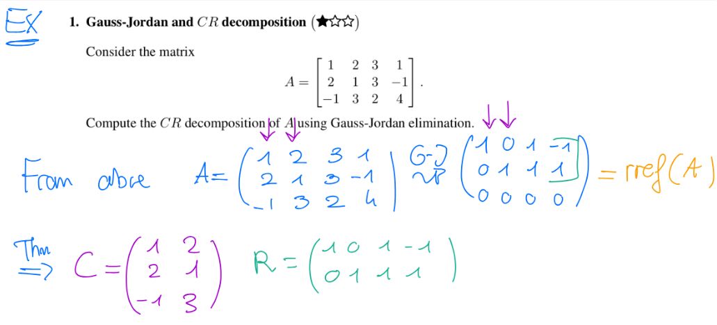
Current
Note has been deleted
Field-by-field Comparison
| Field | Before | After |
|---|---|---|
| Front | ||
| Back |
Note 1307: ETH::1. Semester::LinAlg
Deck: ETH::1. Semester::LinAlg
Note Type: Horvath Cloze
GUID:
deleted
Note Type: Horvath Cloze
GUID:
PtQN)*utrU
Deleted Note
Front
Let \(V, W\) be orthogonal subspaces of \(\mathbb{R}^n\). Then the following statements are equivalent:
- \(W = V^\perp\)
- \(\dim(V) + \dim(W) = n\)
- {{c3::Every \(u \in \mathbb{R}^n\) can be written as \(u = v + w\) with unique vectors \(v \in V\), \(w \in W\)}}
Back
Let \(V, W\) be orthogonal subspaces of \(\mathbb{R}^n\). Then the following statements are equivalent:
- \(W = V^\perp\)
- \(\dim(V) + \dim(W) = n\)
- {{c3::Every \(u \in \mathbb{R}^n\) can be written as \(u = v + w\) with unique vectors \(v \in V\), \(w \in W\)}}
In words, this means that we can combine two orthogonal subspaces and create a new subspace, whose dimension is the sum of the two dimensions.
Current
Note has been deleted
Field-by-field Comparison
| Field | Before | After |
|---|---|---|
| Text | ||
| Extra |
Note 1308: ETH::1. Semester::LinAlg
Deck: ETH::1. Semester::LinAlg
Note Type: Horvath Cloze
GUID:
deleted
Note Type: Horvath Cloze
GUID:
Q!k}HCQCjt
Deleted Note
Front
For all \(n \geq 2\), exactly half of the permutations have sign \(1\) and the rest have sign \(-1\).
Back
For all \(n \geq 2\), exactly half of the permutations have sign \(1\) and the rest have sign \(-1\).
Current
Note has been deleted
Field-by-field Comparison
| Field | Before | After |
|---|---|---|
| Text |
Note 1309: ETH::1. Semester::LinAlg
Deck: ETH::1. Semester::LinAlg
Note Type: Horvath Classic
GUID:
deleted
Note Type: Horvath Classic
GUID:
Q&0Jp*eAqN
Deleted Note
Front
How can we use Gauss-Jordan to simplify the determinant calculations?
Back
How can we use Gauss-Jordan to simplify the determinant calculations?
We can use Gauss-Jordan to make any matrix upper triangular (then the determinant is the product of the diagonals).
We are allowed to use:
We are allowed to use:
- Row addition / substraction
- Exchanging rows (change sign)
- Multiply rows (multiply the determinant at the end)
Current
Note has been deleted
Field-by-field Comparison
| Field | Before | After |
|---|---|---|
| Front | ||
| Back |
Note 1310: ETH::1. Semester::LinAlg
Deck: ETH::1. Semester::LinAlg
Note Type: Horvath Cloze
GUID:
deleted
Note Type: Horvath Cloze
GUID:
Q:@axRgARJ
Deleted Note
Front
Given a square matrix \(A \in \mathbb{R}^{n \times n}\), the determinant \(\det(A)\) is defined as: \[ \det(A) = {{c1:: \sum_{\sigma \in \Pi_n} \text{sgn}(\sigma) \prod_{i = 1}^n A_{i, \sigma(j)} }}\] where \(\Pi_n\) is the set of all permutations of \(n\) elements (of which there are \(n!\)).
Back
Given a square matrix \(A \in \mathbb{R}^{n \times n}\), the determinant \(\det(A)\) is defined as: \[ \det(A) = {{c1:: \sum_{\sigma \in \Pi_n} \text{sgn}(\sigma) \prod_{i = 1}^n A_{i, \sigma(j)} }}\] where \(\Pi_n\) is the set of all permutations of \(n\) elements (of which there are \(n!\)).
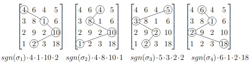
Current
Note has been deleted
Field-by-field Comparison
| Field | Before | After |
|---|---|---|
| Text | ||
| Extra |
Note 1311: ETH::1. Semester::LinAlg
Deck: ETH::1. Semester::LinAlg
Note Type: Horvath Cloze
GUID:
deleted
Note Type: Horvath Cloze
GUID:
Q<9{&+m4lf
Deleted Note
Front
For \(A\) a matrix and \(M\) an invertible matrix:
Back
For \(A\) a matrix and \(M\) an invertible matrix:
\(\begin{bmatrix} 1 & 2 \\ 2 & 4 \end{bmatrix}\) after RREF is \(\begin{bmatrix} 1 & 2 \\ 0 & 0 \end{bmatrix}\) which spans a completely different line.
Current
Note has been deleted
Field-by-field Comparison
| Field | Before | After |
|---|---|---|
| Text | ||
| Extra |
Note 1312: ETH::1. Semester::LinAlg
Deck: ETH::1. Semester::LinAlg
Note Type: Horvath Cloze
GUID:
deleted
Note Type: Horvath Cloze
GUID:
QGIRdw&4iR
Deleted Note
Front
For \(A \in \mathbb{R}^{m \times n}\) with \(\text{rank}(A) = n\), the pseudoinverse \(A^\dagger\) is a left inverse of \(A\), meaning: \[ A^\dagger A = I \]Proof Included
Back
For \(A \in \mathbb{R}^{m \times n}\) with \(\text{rank}(A) = n\), the pseudoinverse \(A^\dagger\) is a left inverse of \(A\), meaning: \[ A^\dagger A = I \]Proof Included
Proof: Since \(A\) has full column rank, \(A^\top A\) invertible and then \(A^\dagger A = ((A^\top A)^{-1} A^\top)A\) \(= (A^\top A)^{-1} (A^\top A) = I\).
Current
Note has been deleted
Field-by-field Comparison
| Field | Before | After |
|---|---|---|
| Text | ||
| Extra |
Note 1313: ETH::1. Semester::LinAlg
Deck: ETH::1. Semester::LinAlg
Note Type: Horvath Classic
GUID:
deleted
Note Type: Horvath Classic
GUID:
QM2twywAT5
Deleted Note
Front
Do the rank or independent columns change if we re-order the columns?
Back
Do the rank or independent columns change if we re-order the columns?
The independent columns change, but not their number and thus not the rank.
Current
Note has been deleted
Field-by-field Comparison
| Field | Before | After |
|---|---|---|
| Front | ||
| Back |
Note 1314: ETH::1. Semester::LinAlg
Deck: ETH::1. Semester::LinAlg
Note Type: Horvath Cloze
GUID:
deleted
Note Type: Horvath Cloze
GUID:
QlPn|vP;}Y
Deleted Note
Front
The Gram matrix of \(V \in \mathbb{R}^{n \times n}\) is \(G = V^\top V\).
Back
The Gram matrix of \(V \in \mathbb{R}^{n \times n}\) is \(G = V^\top V\).
Current
Note has been deleted
Field-by-field Comparison
| Field | Before | After |
|---|---|---|
| Text |
Note 1315: ETH::1. Semester::LinAlg
Deck: ETH::1. Semester::LinAlg
Note Type: Horvath Cloze
GUID:
deleted
Note Type: Horvath Cloze
GUID:
Qn=Bf?WQ4E
Deleted Note
Front
Dimension of the left-nullspace \(\dim(\textbf{N}(A^\top)) = \){{c1::\(m - r = m - \textbf{rank}(A)\)}}.
Back
Dimension of the left-nullspace \(\dim(\textbf{N}(A^\top)) = \){{c1::\(m - r = m - \textbf{rank}(A)\)}}.
Current
Note has been deleted
Field-by-field Comparison
| Field | Before | After |
|---|---|---|
| Text |
Note 1316: ETH::1. Semester::LinAlg
Deck: ETH::1. Semester::LinAlg
Note Type: Horvath Classic
GUID:
deleted
Note Type: Horvath Classic
GUID:
Qp5sodd?T?
Deleted Note
Front
When is a function considered to be a linear transformation or a linear functional?
Back
When is a function considered to be a linear transformation or a linear functional?
If the linearity axiom holds for it:
\(T(\lambda_1x_1 + \lambda_2x_2) = \lambda_1T(x_1) + \lambda_2T(x_2)\)
\(T(\lambda_1x_1 + \lambda_2x_2) = \lambda_1T(x_1) + \lambda_2T(x_2)\)
Current
Note has been deleted
Field-by-field Comparison
| Field | Before | After |
|---|---|---|
| Front | ||
| Back |
Note 1317: ETH::1. Semester::LinAlg
Deck: ETH::1. Semester::LinAlg
Note Type: Horvath Classic
GUID:
deleted
Note Type: Horvath Classic
GUID:
Z|WywzzA)
Deleted Note
Front
We can get the unit vector for every single vector \(\textbf{v}\) by
Back
We can get the unit vector for every single vector \(\textbf{v}\) by
dividing by the norm of the vector: \(\frac{\textbf{v}}{||\textbf{v}||}\).
Current
Note has been deleted
Field-by-field Comparison
| Field | Before | After |
|---|---|---|
| Front | ||
| Back |
Note 1318: ETH::1. Semester::LinAlg
Deck: ETH::1. Semester::LinAlg
Note Type: Horvath Cloze
GUID:
deleted
Note Type: Horvath Cloze
GUID:
b$)8Q]2TlG
Deleted Note
Front
\(A\) is invertible if and only if there exists \(B\) such that \(AB = BA = I\),
Back
\(A\) is invertible if and only if there exists \(B\) such that \(AB = BA = I\),
Current
Note has been deleted
Field-by-field Comparison
| Field | Before | After |
|---|---|---|
| Text |
Note 1319: ETH::1. Semester::LinAlg
Deck: ETH::1. Semester::LinAlg
Note Type: Horvath Cloze
GUID:
deleted
Note Type: Horvath Cloze
GUID:
b-hsvze>Y9
Deleted Note
Front
For \(A \in \mathbb{R}^{m \times n}\) with \(\text{rank}(A) = n\), we define the pseudo-inverse \(A^\dagger \in \mathbb{R}^{n \times m}\) as \[ A^\dagger = {{c1::(A^\top A)^{-1} A^\top }}\]
Back
For \(A \in \mathbb{R}^{m \times n}\) with \(\text{rank}(A) = n\), we define the pseudo-inverse \(A^\dagger \in \mathbb{R}^{n \times m}\) as \[ A^\dagger = {{c1::(A^\top A)^{-1} A^\top }}\]
Current
Note has been deleted
Field-by-field Comparison
| Field | Before | After |
|---|---|---|
| Text |
Note 1320: ETH::1. Semester::LinAlg
Deck: ETH::1. Semester::LinAlg
Note Type: Horvath Cloze
GUID:
deleted
Note Type: Horvath Cloze
GUID:
b84e;HsPv=
Deleted Note
Front
A real valued matrix \(A \in \mathbb{R}^{n \times n}\) has real or complex valued eigenvalues.
Back
A real valued matrix \(A \in \mathbb{R}^{n \times n}\) has real or complex valued eigenvalues.
Current
Note has been deleted
Field-by-field Comparison
| Field | Before | After |
|---|---|---|
| Text |
Note 1321: ETH::1. Semester::LinAlg
Deck: ETH::1. Semester::LinAlg
Note Type: Horvath Cloze
GUID:
deleted
Note Type: Horvath Cloze
GUID:
bE;:bQU7h5
Deleted Note
Front
If \(Ax = b\) has a solution, then \(\textbf{Sol}(A, b)\) has dimension \(n - r\), where \[ \dim(\textbf{Sol}(A, b)) := {{c1::\dim(\textbf{N}(A)) }}\]
Back
If \(Ax = b\) has a solution, then \(\textbf{Sol}(A, b)\) has dimension \(n - r\), where \[ \dim(\textbf{Sol}(A, b)) := {{c1::\dim(\textbf{N}(A)) }}\]
Current
Note has been deleted
Field-by-field Comparison
| Field | Before | After |
|---|---|---|
| Text |
Note 1322: ETH::1. Semester::LinAlg
Deck: ETH::1. Semester::LinAlg
Note Type: Horvath Cloze
GUID:
deleted
Note Type: Horvath Cloze
GUID:
bERVf5Y&x?
Deleted Note
Front
Let \(V\) be a finitely generated vector space and let \(G \subseteq V\) be a finite subset with \(\textbf{Span}(G) = V\).
Then \(V\) has a basis \(B \subseteq G\).
Then \(V\) has a basis \(B \subseteq G\).
Back
Let \(V\) be a finitely generated vector space and let \(G \subseteq V\) be a finite subset with \(\textbf{Span}(G) = V\).
Then \(V\) has a basis \(B \subseteq G\).
Then \(V\) has a basis \(B \subseteq G\).
Current
Note has been deleted
Field-by-field Comparison
| Field | Before | After |
|---|---|---|
| Text |
Note 1323: ETH::1. Semester::LinAlg
Deck: ETH::1. Semester::LinAlg
Note Type: Horvath Cloze
GUID:
deleted
Note Type: Horvath Cloze
GUID:
bJ-+lUD,dW
Deleted Note
Front
Because \(R(A) = C(A^\top)\) and \(N(A)\) are orthogonal, we can decompose any vector \(x \in \mathbb{R}^n\) into \(x = x_r + x_n\) where \(x_r \in R(A) \) is unique and \(x_n \in N(A)\) can be any value.
Back
Because \(R(A) = C(A^\top)\) and \(N(A)\) are orthogonal, we can decompose any vector \(x \in \mathbb{R}^n\) into \(x = x_r + x_n\) where \(x_r \in R(A) \) is unique and \(x_n \in N(A)\) can be any value.
We can take any \(x_n \in N(A)\) because when doing \(Ax = Ax_r + Ax_n = Ax_r\) as \(Ax_n = 0\).
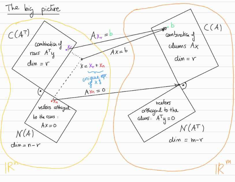
Current
Note has been deleted
Field-by-field Comparison
| Field | Before | After |
|---|---|---|
| Text | ||
| Extra |
Note 1324: ETH::1. Semester::LinAlg
Deck: ETH::1. Semester::LinAlg
Note Type: Horvath Classic
GUID:
deleted
Note Type: Horvath Classic
GUID:
cUvvD`tlgp
Deleted Note
Front
What happens in the case of linearly dependent vectors in \(A\) during Gram-Schmidt?
Back
What happens in the case of linearly dependent vectors in \(A\) during Gram-Schmidt?
Since in a linearly dependent set of vectors one of them is a linear combination of the previous ones, you'd get \(0\) in the subtraction step for it. By excluding those \(0\)'s you'd still get an orthonormal basis.
Current
Note has been deleted
Field-by-field Comparison
| Field | Before | After |
|---|---|---|
| Front | ||
| Back |
Note 1325: ETH::1. Semester::LinAlg
Deck: ETH::1. Semester::LinAlg
Note Type: Horvath Cloze
GUID:
deleted
Note Type: Horvath Cloze
GUID:
cX#._>C>2&
Deleted Note
Front
Certificate of no solutions:\[ \{x \in \mathbb{R}^n \ | \ Ax = b \} = \emptyset\]is equivalent to:
\[{{c1:: \{z \in \mathbb{R}^m \ | \ A^\top z = 0, b^\top z = 1 \} \not = \emptyset }}\]
Note that we don’t need it to be \(1\), it just has to be \(\neq 0\).
Back
Certificate of no solutions:\[ \{x \in \mathbb{R}^n \ | \ Ax = b \} = \emptyset\]is equivalent to:
\[{{c1:: \{z \in \mathbb{R}^m \ | \ A^\top z = 0, b^\top z = 1 \} \not = \emptyset }}\]
Note that we don’t need it to be \(1\), it just has to be \(\neq 0\).
In words: our LSE \(Ax = b\) does not have any solutions if and only if there exists a vector \(z\) that is orthogonal to all columns of \(A\) but not orthogonal to \(b\).
The blue vector \(z\) is orthogonal to all in \(C(A)\), the blue subspace.
If \(b\) is not orthogonal to \(z\), this means that it cannot possibly be in the subspace, it must be slightly above/below it. Therefore \(b \not \in C(A)\) and thus there's no solution.
The blue vector \(z\) is orthogonal to all in \(C(A)\), the blue subspace.
If \(b\) is not orthogonal to \(z\), this means that it cannot possibly be in the subspace, it must be slightly above/below it. Therefore \(b \not \in C(A)\) and thus there's no solution.
Current
Note has been deleted
Field-by-field Comparison
| Field | Before | After |
|---|---|---|
| Text | ||
| Extra |
Note 1326: ETH::1. Semester::LinAlg
Deck: ETH::1. Semester::LinAlg
Note Type: Horvath Cloze
GUID:
deleted
Note Type: Horvath Cloze
GUID:
col^b$YzMt
Deleted Note
Front
\(v^\top v = \) \(||v||^2\)
Back
\(v^\top v = \) \(||v||^2\)
as \(||v|| = \sqrt{v^\top v}\).
Current
Note has been deleted
Field-by-field Comparison
| Field | Before | After |
|---|---|---|
| Text | ||
| Extra |
Note 1327: ETH::1. Semester::LinAlg
Deck: ETH::1. Semester::LinAlg
Note Type: Horvath Classic
GUID:
deleted
Note Type: Horvath Classic
GUID:
d4<]X?O^},
Deleted Note
Front
When is \(0 \in \textbf{Span}(\{v_1, \dots, v_n\})\)?
Back
When is \(0 \in \textbf{Span}(\{v_1, \dots, v_n\})\)?
\(0\) is in the span of any vectors, even in the span of the empty set.
Current
Note has been deleted
Field-by-field Comparison
| Field | Before | After |
|---|---|---|
| Front | ||
| Back |
Note 1328: ETH::1. Semester::LinAlg
Deck: ETH::1. Semester::LinAlg
Note Type: Horvath Classic
GUID:
deleted
Note Type: Horvath Classic
GUID:
d8[ROk!
Deleted Note
Front
To compute the CR decomposition, we:
Back
To compute the CR decomposition, we:
Compute the RREF of \(A\)
- Get \(C\) by taking the independent columns of \(A\) (those corresponding to the pivot columns in RREF)
- Get \(R'\) by removing the \(0\) rows of the RREF form of \(A\).
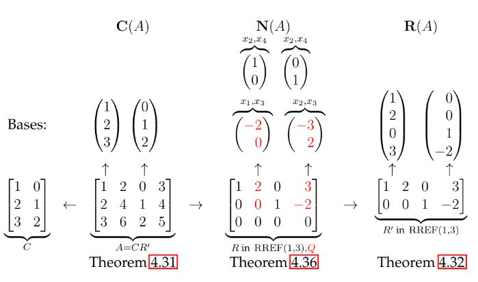
Current
Note has been deleted
Field-by-field Comparison
| Field | Before | After |
|---|---|---|
| Front | ||
| Back |
Note 1329: ETH::1. Semester::LinAlg
Deck: ETH::1. Semester::LinAlg
Note Type: Horvath Cloze
GUID:
deleted
Note Type: Horvath Cloze
GUID:
d8bL*1FU!1
Deleted Note
Front
For \(A\) an \(m \times n\) matrix, we have:
\( \textbf{rank}(A) = \textbf{rank}(A^\top) \)
\( \textbf{rank}(A) = \textbf{rank}(A^\top) \)
Back
For \(A\) an \(m \times n\) matrix, we have:
\( \textbf{rank}(A) = \textbf{rank}(A^\top) \)
\( \textbf{rank}(A) = \textbf{rank}(A^\top) \)
Current
Note has been deleted
Field-by-field Comparison
| Field | Before | After |
|---|---|---|
| Text |
Note 1330: ETH::1. Semester::LinAlg
Deck: ETH::1. Semester::LinAlg
Note Type: Horvath Cloze
GUID:
deleted
Note Type: Horvath Cloze
GUID:
d9#?3c)V#_
Deleted Note
Front
Let \(A \in \mathbb{R}^{n \times n}\) be a symmetric matrix and \(\lambda \in \mathbb{C}\) be an eigenvalue of \(A\), then {{c1::\(\lambda \in \mathbb{R}\)::property of the EW}}. Proof Included
Back
Let \(A \in \mathbb{R}^{n \times n}\) be a symmetric matrix and \(\lambda \in \mathbb{C}\) be an eigenvalue of \(A\), then {{c1::\(\lambda \in \mathbb{R}\)::property of the EW}}. Proof Included
Proof \(v \in \mathbb{C}^n\) be EV of \(\lambda\). Thus we have \(Av = \lambda v\). Since \(A\) is symmetric we have \(A^ = A\). \[\begin{align} \overline{\lambda}||v||^2 &= \overline{\lambda} v^*v \\ &= (\lambda v)^*v \\ &= (Av)^*v = v^*A^*v \\ &= v^* Av \text{ (uses } A^* = A \text{) } \\ &= v^*\lambda v \\ &= \lambda ||v||^2 \end{align}\]Since \(v \neq 0\), then \(||v|| \neq 0\) and so \(\lambda = \overline{\lambda}\) thus \(\lambda \in \mathbb{R}\).
Current
Note has been deleted
Field-by-field Comparison
| Field | Before | After |
|---|---|---|
| Text | ||
| Extra |
Note 1331: ETH::1. Semester::LinAlg
Deck: ETH::1. Semester::LinAlg
Note Type: Horvath Cloze
GUID:
deleted
Note Type: Horvath Cloze
GUID:
d?+tf|$hUH
Deleted Note
Front
\(A\) is invertible if and only if for \(\text{RREF}(A,I) = (R, M)\) we have \(R = I\).
Back
\(A\) is invertible if and only if for \(\text{RREF}(A,I) = (R, M)\) we have \(R = I\).
Since we have \(R = MA\), \(M\) is the inverse of \(A\).
Current
Note has been deleted
Field-by-field Comparison
| Field | Before | After |
|---|---|---|
| Text | ||
| Extra |
Note 1332: ETH::1. Semester::LinAlg
Deck: ETH::1. Semester::LinAlg
Note Type: Horvath Cloze
GUID:
deleted
Note Type: Horvath Cloze
GUID:
dET3O3a8?c
Deleted Note
Front
A minimiser of \(\min_{\hat{x} \in \mathbb{R}^n} || A\hat{x} - b||^2\) is also a solution of \(A^\top A \hat{x} = A^\top b\).
When \(A\) has independent columns the unique minimiser of \(\hat{x}\) is given by: \[ \hat{x} = {{c2::(A^\top A)^{-1} A^\top b }}\]
Back
A minimiser of \(\min_{\hat{x} \in \mathbb{R}^n} || A\hat{x} - b||^2\) is also a solution of \(A^\top A \hat{x} = A^\top b\).
When \(A\) has independent columns the unique minimiser of \(\hat{x}\) is given by: \[ \hat{x} = {{c2::(A^\top A)^{-1} A^\top b }}\]
Current
Note has been deleted
Field-by-field Comparison
| Field | Before | After |
|---|---|---|
| Text |
Note 1333: ETH::1. Semester::LinAlg
Deck: ETH::1. Semester::LinAlg
Note Type: Horvath Cloze
GUID:
deleted
Note Type: Horvath Cloze
GUID:
dZ)aTr>2eb
Deleted Note
Front
Given a real matrix \(A \in \mathbb{R}^{n \times n}\), the non-zero eigenvalues of \(A^\top A\) are the same ones as of \(AA^\top\). Proof Included
Back
Given a real matrix \(A \in \mathbb{R}^{n \times n}\), the non-zero eigenvalues of \(A^\top A\) are the same ones as of \(AA^\top\). Proof Included
Shared EWs: For \((A^\top A)v_k = \lambda_k v_k\) we get \(AA^\top A v_k = \lambda_k Av_k\) and thus \(Av_k\) EV and \(\lambda_k\) is an EW of \(AA^\top\).
Orthogonality: For \(j \neq k\) we have \((Av_j)^\top (Av_k) = v_j^\top A^\top Av_k = v_j^\top \lambda_k v_k = \lambda_k v_j^\top v_k = 0\)
Orthogonality: For \(j \neq k\) we have \((Av_j)^\top (Av_k) = v_j^\top A^\top Av_k = v_j^\top \lambda_k v_k = \lambda_k v_j^\top v_k = 0\)
Current
Note has been deleted
Field-by-field Comparison
| Field | Before | After |
|---|---|---|
| Text | ||
| Extra |
Note 1334: ETH::1. Semester::LinAlg
Deck: ETH::1. Semester::LinAlg
Note Type: Horvath Classic
GUID:
deleted
Note Type: Horvath Classic
GUID:
d[`]Ch#J!c
Deleted Note
Front
What is the fundamental theorem of algebra?
Back
What is the fundamental theorem of algebra?
Any degree \(n\) polynomial \(P(z) = a_n z^n + a_{n-1} z^{n-1} + \dots + a_1 z + a_0\) (with \(n \geq 1\) and \(a_n \neq 0\)) has at least one zero \(\lambda \in \mathbb{C}\) such that \(P(\lambda) = 0\).
Current
Note has been deleted
Field-by-field Comparison
| Field | Before | After |
|---|---|---|
| Front | ||
| Back |
Note 1335: ETH::1. Semester::LinAlg
Deck: ETH::1. Semester::LinAlg
Note Type: Horvath Cloze
GUID:
deleted
Note Type: Horvath Cloze
GUID:
db7R/9=X)q
Deleted Note
Front
Suppose that \(\{x \in \mathbb{R}^n \ | \ Ax = b \} \not = \emptyset\). Then \[ \{x \in \mathbb{R}^n \ | \ Ax = b \} = x_1 + N(A) \] where \(x_1 \in R(A)\) is unique such that \(Ax_1 = b\).
Back
Suppose that \(\{x \in \mathbb{R}^n \ | \ Ax = b \} \not = \emptyset\). Then \[ \{x \in \mathbb{R}^n \ | \ Ax = b \} = x_1 + N(A) \] where \(x_1 \in R(A)\) is unique such that \(Ax_1 = b\).
This means that if there's more than one solution to the system (i.e. the nullspace is not \(= \{0\}\)), then the set of all solutions is a specific solution + the entire nullspace.
Current
Note has been deleted
Field-by-field Comparison
| Field | Before | After |
|---|---|---|
| Text | ||
| Extra |
Note 1336: ETH::1. Semester::LinAlg
Deck: ETH::1. Semester::LinAlg
Note Type: Horvath Cloze
GUID:
deleted
Note Type: Horvath Cloze
GUID:
dkbvj2%i-%
Deleted Note
Front
A real EV always has a real EW associated with it.
Back
A real EV always has a real EW associated with it.
Current
Note has been deleted
Field-by-field Comparison
| Field | Before | After |
|---|---|---|
| Text |
Note 1337: ETH::1. Semester::LinAlg
Deck: ETH::1. Semester::LinAlg
Note Type: Horvath Classic
GUID:
deleted
Note Type: Horvath Classic
GUID:
dle9WT5o|g
Deleted Note
Front
What is the pseudoinverse in the case where \(A \in \mathbb{R}^{n \times m}\) has independent rows?
Back
What is the pseudoinverse in the case where \(A \in \mathbb{R}^{n \times m}\) has independent rows?
Because \(rank(A) = r = m\) and thus \(n \geq m\)
We know \(x = x_r + x_n\) for \(x_r \in R(A)\) and \(x_n \in N(A)\) thus we pick \(x = x_r + 0\) to get the smallest norm.
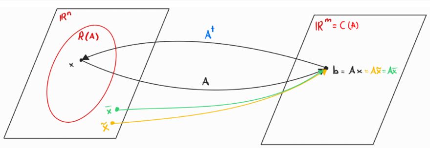
- \(C(A)\) spans \(\mathbb{R}^m\) (columns span the space)
- \(R(A) \subseteq\) \(\mathbb{R}^n\)
We know \(x = x_r + x_n\) for \(x_r \in R(A)\) and \(x_n \in N(A)\) thus we pick \(x = x_r + 0\) to get the smallest norm.
Current
Note has been deleted
Field-by-field Comparison
| Field | Before | After |
|---|---|---|
| Front | ||
| Back |
Note 1338: ETH::1. Semester::LinAlg
Deck: ETH::1. Semester::LinAlg
Note Type: Horvath Cloze
GUID:
deleted
Note Type: Horvath Cloze
GUID:
dmvZr9zGs8
Deleted Note
Front
A diagonal matrix has it's EWs on the diagonal.
Back
A diagonal matrix has it's EWs on the diagonal.
Current
Note has been deleted
Field-by-field Comparison
| Field | Before | After |
|---|---|---|
| Text |
Note 1339: ETH::1. Semester::LinAlg
Deck: ETH::1. Semester::LinAlg
Note Type: Horvath Cloze
GUID:
deleted
Note Type: Horvath Cloze
GUID:
doaX+*9B4:
Deleted Note
Front
For an eigenvalue \(\lambda\) of \(M\), \(\lambda + c\) is a real eigenvalue of the matrix \(M + cI\).
Back
For an eigenvalue \(\lambda\) of \(M\), \(\lambda + c\) is a real eigenvalue of the matrix \(M + cI\).
Intuitively this makes sense as by adding \(cI\) we're increasing the values on the diagonal, meaning we have to increase the value of \(\lambda\) by the same amount so that we get \(0\) again.
Current
Note has been deleted
Field-by-field Comparison
| Field | Before | After |
|---|---|---|
| Text | ||
| Extra |
Note 1340: ETH::1. Semester::LinAlg
Deck: ETH::1. Semester::LinAlg
Note Type: Horvath Classic
GUID:
deleted
Note Type: Horvath Classic
GUID:
dsS2q:x~S{
Deleted Note
Front
Why does \(QR\) give \(A\)?
Back
Why does \(QR\) give \(A\)?
\(QQ^\top\) is the projection on the span of the \(q_i\)'s and thus also on the \(a_i\)'s (\(C(Q) = C(A)\)).
Thus \(QQ^\top A = A\) and therefore \(QR = QQ^\top A = A\).
Thus \(QQ^\top A = A\) and therefore \(QR = QQ^\top A = A\).
Current
Note has been deleted
Field-by-field Comparison
| Field | Before | After |
|---|---|---|
| Front | ||
| Back |
Note 1341: ETH::1. Semester::LinAlg
Deck: ETH::1. Semester::LinAlg
Note Type: Horvath Cloze
GUID:
deleted
Note Type: Horvath Cloze
GUID:
e#C4kgY#N_
Deleted Note
Front
If \(b \neq 0\), \(\textbf{Sol}(A, b)\) is {{c1::not a subspace of \(\mathbb{R}^n\)}}.
Back
If \(b \neq 0\), \(\textbf{Sol}(A, b)\) is {{c1::not a subspace of \(\mathbb{R}^n\)}}.
Because it doesn't contain the zero vector!
If \(b \neq 0\), the the solution space is "shifted" off the origin:
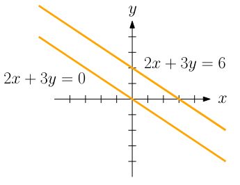
If \(b \neq 0\), the the solution space is "shifted" off the origin:
Current
Note has been deleted
Field-by-field Comparison
| Field | Before | After |
|---|---|---|
| Text | ||
| Extra |
Note 1342: ETH::1. Semester::LinAlg
Deck: ETH::1. Semester::LinAlg
Note Type: Horvath Cloze
GUID:
deleted
Note Type: Horvath Cloze
GUID:
e?j,2#~.l4
Deleted Note
Front
Let \(S\) be a subspace in \(\mathbb{R}^m\) and \(A\) a matrix whose columns are a basis of \(S\).
The projection matrix \(P\) to a matrix \(A\) is given by: {{c1::\(P = A (A^\top A)^{-1} A^\top\)}}
The projection of \(b \in \mathbb{R}^m\) to \(S\) is given by \(\text{proj}_S(b) = Pb\).
The projection matrix \(P\) to a matrix \(A\) is given by: {{c1::\(P = A (A^\top A)^{-1} A^\top\)}}
The projection of \(b \in \mathbb{R}^m\) to \(S\) is given by \(\text{proj}_S(b) = Pb\).
Back
Let \(S\) be a subspace in \(\mathbb{R}^m\) and \(A\) a matrix whose columns are a basis of \(S\).
The projection matrix \(P\) to a matrix \(A\) is given by: {{c1::\(P = A (A^\top A)^{-1} A^\top\)}}
The projection of \(b \in \mathbb{R}^m\) to \(S\) is given by \(\text{proj}_S(b) = Pb\).
The projection matrix \(P\) to a matrix \(A\) is given by: {{c1::\(P = A (A^\top A)^{-1} A^\top\)}}
The projection of \(b \in \mathbb{R}^m\) to \(S\) is given by \(\text{proj}_S(b) = Pb\).
Note the condition for the columns to be a basis - this forces them to be independent, which means \(A^\top A\) invertible by Lemma 5.2.4.
Current
Note has been deleted
Field-by-field Comparison
| Field | Before | After |
|---|---|---|
| Text | ||
| Extra |
Note 1343: ETH::1. Semester::LinAlg
Deck: ETH::1. Semester::LinAlg
Note Type: Horvath Classic
GUID:
deleted
Note Type: Horvath Classic
GUID:
eGgKwc!Y>B
Deleted Note
Front
Was ist eine orthogonale Matrix?
Back
Was ist eine orthogonale Matrix?
Für eine orthogonale Matrix gilt \( \mathbf{A^\top A = I}_n\), d.h. die Inverse von A ist A transponiert. Orthogonal = reell, quadratisch, regulär
Current
Note has been deleted
Field-by-field Comparison
| Field | Before | After |
|---|---|---|
| Front | ||
| Back |
Note 1344: ETH::1. Semester::LinAlg
Deck: ETH::1. Semester::LinAlg
Note Type: Horvath Classic
GUID:
deleted
Note Type: Horvath Classic
GUID:
eUCQYkiYf@
Deleted Note
Front
What is a property that always holds for linear transformations?
Back
What is a property that always holds for linear transformations?
\(T(0) = 0\)
Current
Note has been deleted
Field-by-field Comparison
| Field | Before | After |
|---|---|---|
| Front | ||
| Back |
Note 1345: ETH::1. Semester::LinAlg
Deck: ETH::1. Semester::LinAlg
Note Type: Horvath Cloze
GUID:
deleted
Note Type: Horvath Cloze
GUID:
eY$X2~xJ5/
Deleted Note
Front
Name the three definitions for linear independence:
- None of the vectors is a linear combination of the other ones.
- {{c2::There are no scalars \(\lambda_1, ..., \lambda_n\) besides 0, 0, ..., 0 such that \(\sum_{i = 1}^n \lambda_i v_i = \mathbf{0}\). (\(\mathbf{0}\) can only be written as a trivial combination of the vectors.)}}
- None of the vectors is a linear combination of the previous ones.
Back
Name the three definitions for linear independence:
- None of the vectors is a linear combination of the other ones.
- {{c2::There are no scalars \(\lambda_1, ..., \lambda_n\) besides 0, 0, ..., 0 such that \(\sum_{i = 1}^n \lambda_i v_i = \mathbf{0}\). (\(\mathbf{0}\) can only be written as a trivial combination of the vectors.)}}
- None of the vectors is a linear combination of the previous ones.
Current
Note has been deleted
Field-by-field Comparison
| Field | Before | After |
|---|---|---|
| Text |
Note 1346: ETH::1. Semester::LinAlg
Deck: ETH::1. Semester::LinAlg
Note Type: Horvath Classic
GUID:
deleted
Note Type: Horvath Classic
GUID:
e`7dX^~/:X
Deleted Note
Front
For a function \(T: \mathbb{R}^n \rightarrow \mathbb{R}^m / \ T: \mathbb{R}^n \rightarrow \mathbb{R}\) the linearity axiom is:
Back
For a function \(T: \mathbb{R}^n \rightarrow \mathbb{R}^m / \ T: \mathbb{R}^n \rightarrow \mathbb{R}\) the linearity axiom is:
\(T(\lambda_1x_1 + \lambda_2x_2) = \lambda_1T(x_1) + \lambda_2T(x_2)\)
Current
Note has been deleted
Field-by-field Comparison
| Field | Before | After |
|---|---|---|
| Front | ||
| Back |
Note 1347: ETH::1. Semester::LinAlg
Deck: ETH::1. Semester::LinAlg
Note Type: Horvath Cloze
GUID:
deleted
Note Type: Horvath Cloze
GUID:
eb|cwXEzx`
Deleted Note
Front
A \(m\times 1\) matrix is called a column vector.
Back
A \(m\times 1\) matrix is called a column vector.
Current
Note has been deleted
Field-by-field Comparison
| Field | Before | After |
|---|---|---|
| Text |
Note 1348: ETH::1. Semester::LinAlg
Deck: ETH::1. Semester::LinAlg
Note Type: Horvath Cloze
GUID:
deleted
Note Type: Horvath Cloze
GUID:
er&wX,XKn1
Deleted Note
Front
Every symmetric PSD matrix \(M\) is a Gram matrix of an upper triangular matrix \(C\).
\(M = C^\top C\) is known as the Cholesky decomposition.
Proof Included
\(M = C^\top C\) is known as the Cholesky decomposition.
Proof Included
Back
Every symmetric PSD matrix \(M\) is a Gram matrix of an upper triangular matrix \(C\).
\(M = C^\top C\) is known as the Cholesky decomposition.
Proof Included
\(M = C^\top C\) is known as the Cholesky decomposition.
Proof Included
Thus all PSD matrices are decomposable as \(C^\top C\) with \(C\) upper triangular!
Proof: Since \(M\) is symmetric PSD, we can say \(M = V \Lambda V^\top\) with \(\Lambda\) diagonal matrix with EWs in the diagonal.
- Since \(M\) is PSD, the eigenvalues (the diagonals) of \(\Lambda\) are \(\geq 0\) (non-negative) and thus we can build \(\Lambda^{1/2}\) by taking the square root of each diagonal entry.
- To make them be upper triangular, we take the QR-decomposition (\(V\Lambda^{1/2}\) has linearly independent columns) \((V \Lambda^{1/2})^\top = QR\) with \(Q\) such that \(Q^\top Q = I\) and \(R\) upper triangular.
- We then have \(M = (V \Lambda^{1/2})(V \Lambda^{1/2})^\top\)\( = (QR)^\top (QR) = \)\(R^\top Q^\top Q R = R^\top R\)
Taking \(C = R\) we get \(M = C^\top C\).
Current
Note has been deleted
Field-by-field Comparison
| Field | Before | After |
|---|---|---|
| Text | ||
| Extra |
Note 1349: ETH::1. Semester::LinAlg
Deck: ETH::1. Semester::LinAlg
Note Type: Horvath Cloze
GUID:
deleted
Note Type: Horvath Cloze
GUID:
eybQSQ#Ama
Deleted Note
Front
The eigenvectors of \(A\) are not the same as those of \(A^\top\).
Back
The eigenvectors of \(A\) are not the same as those of \(A^\top\).
Current
Note has been deleted
Field-by-field Comparison
| Field | Before | After |
|---|---|---|
| Text |
Note 1350: ETH::1. Semester::LinAlg
Deck: ETH::1. Semester::LinAlg
Note Type: Horvath Cloze
GUID:
deleted
Note Type: Horvath Cloze
GUID:
f&MFQatooW
Deleted Note
Front
The \(\det\) of \(U\) upper (or lower) triangular is \(\det U = {{c1:: (u_{11})(u_{22}) \dots (u_{nn}) }}\). Intuition included
Back
The \(\det\) of \(U\) upper (or lower) triangular is \(\det U = {{c1:: (u_{11})(u_{22}) \dots (u_{nn}) }}\). Intuition included
(The product of the diagonal entries.)
This is because any permutation except the \(\text{id}\) permutation chooses a \(0\) at least once.
This is because any permutation except the \(\text{id}\) permutation chooses a \(0\) at least once.
Current
Note has been deleted
Field-by-field Comparison
| Field | Before | After |
|---|---|---|
| Text | ||
| Extra |
Note 1351: ETH::1. Semester::LinAlg
Deck: ETH::1. Semester::LinAlg
Note Type: Horvath Classic
GUID:
deleted
Note Type: Horvath Classic
GUID:
f3K7#O4X*v
Deleted Note
Front
Is the empty set of vectors linearly dependent or independent?
Back
Is the empty set of vectors linearly dependent or independent?
It is linearly independent by definition, since there is no vector it could be a combination of.
Current
Note has been deleted
Field-by-field Comparison
| Field | Before | After |
|---|---|---|
| Front | ||
| Back |
Note 1352: ETH::1. Semester::LinAlg
Deck: ETH::1. Semester::LinAlg
Note Type: Horvath Classic
GUID:
deleted
Note Type: Horvath Classic
GUID:
f9O^%9R1}/
Deleted Note
Front
When are two vectors orthogonal?
Back
When are two vectors orthogonal?
When their scalar product is equal to 0.
This means that the projection of v onto w results in a vector v of 0 length.
This means that the projection of v onto w results in a vector v of 0 length.
Current
Note has been deleted
Field-by-field Comparison
| Field | Before | After |
|---|---|---|
| Front | ||
| Back |
Note 1353: ETH::1. Semester::LinAlg
Deck: ETH::1. Semester::LinAlg
Note Type: Horvath Classic
GUID:
deleted
Note Type: Horvath Classic
GUID:
f>Z/u`5f-r
Deleted Note
Front
What does \(N(A) = \{0\}\) mean?
Back
What does \(N(A) = \{0\}\) mean?
That all the columns of the matrix are independent.
Current
Note has been deleted
Field-by-field Comparison
| Field | Before | After |
|---|---|---|
| Front | ||
| Back |
Note 1354: ETH::1. Semester::LinAlg
Deck: ETH::1. Semester::LinAlg
Note Type: Horvath Classic
GUID:
deleted
Note Type: Horvath Classic
GUID:
f?EhyxxJ04
Deleted Note
Front
Rewrite \(A^\dagger = R^\dagger C^\dagger\) in terms of \(A\), \(R\), \(C\):
Back
Rewrite \(A^\dagger = R^\dagger C^\dagger\) in terms of \(A\), \(R\), \(C\):
\(\begin{aligned}
A^\dagger &= R^\top (RR^\top)^{-1} (C^\top C)^{-1} C^\top \\
&= R^\top (C^\top C R R^\top)^{-1} C^\top \\
&= R^\top (C^\top A R^\top)^{-1} C^\top
\end{aligned}\)
Current
Note has been deleted
Field-by-field Comparison
| Field | Before | After |
|---|---|---|
| Front | ||
| Back |
Note 1355: ETH::1. Semester::LinAlg
Deck: ETH::1. Semester::LinAlg
Note Type: Horvath Cloze
GUID:
deleted
Note Type: Horvath Cloze
GUID:
f?VIJc~!G|
Deleted Note
Front
Assume \(Q\) is orthogonal and square. Then:
- \(QQ^\top = I\)
- {{c2::\(Q^{-1} = Q^\top\)}}
- {{c3::The columns form an orthonormal basis for \(\mathbb{R}^n\).}}
Back
Assume \(Q\) is orthogonal and square. Then:
- \(QQ^\top = I\)
- {{c2::\(Q^{-1} = Q^\top\)}}
- {{c3::The columns form an orthonormal basis for \(\mathbb{R}^n\).}}
Current
Note has been deleted
Field-by-field Comparison
| Field | Before | After |
|---|---|---|
| Text |
Note 1356: ETH::1. Semester::LinAlg
Deck: ETH::1. Semester::LinAlg
Note Type: Horvath Cloze
GUID:
deleted
Note Type: Horvath Cloze
GUID:
fILs=r`j+*
Deleted Note
Front
Spectral Theorem: Any symmetric matrix \(A \in \mathbb{R}^{n \times n}\) has \(n\) real eigenvalues and {{c1::an orthonormal basis of \(\mathbb{R}^{n \times n}\) consisting of it's eigenvectors::EV}}.
Back
Spectral Theorem: Any symmetric matrix \(A \in \mathbb{R}^{n \times n}\) has \(n\) real eigenvalues and {{c1::an orthonormal basis of \(\mathbb{R}^{n \times n}\) consisting of it's eigenvectors::EV}}.
Current
Note has been deleted
Field-by-field Comparison
| Field | Before | After |
|---|---|---|
| Text |
Note 1357: ETH::1. Semester::LinAlg
Deck: ETH::1. Semester::LinAlg
Note Type: Horvath Cloze
GUID:
deleted
Note Type: Horvath Cloze
GUID:
fTGz~gZIJt
Deleted Note
Front
If \(A^T A\) is invertible, we have a unique solution \(\hat{x}\) that satisfies the equation: \[ p = A\hat{x} = {{c1:: A (A^\top A)^{-1} A^\top b }}\]
Back
If \(A^T A\) is invertible, we have a unique solution \(\hat{x}\) that satisfies the equation: \[ p = A\hat{x} = {{c1:: A (A^\top A)^{-1} A^\top b }}\]
From \(A^\top A \mathbf{\hat{x}} = A^\top \mathbf{b}\) we can construct a formula for \(\mathbf{p}\):
\((A^\top A)^{-1}(A^\top A) \mathbf{\hat{x}} = (A^\top A)^{-1}A^\top \mathbf{b}\)
(\(A^\top A\) invertible if the columns of \(A\) are independent), which gives us:
\(A \mathbf{\hat{x}} = A (A^\top A)^{-1} A^\top \mathbf{b} = \mathbf{p}\).
\((A^\top A)^{-1}(A^\top A) \mathbf{\hat{x}} = (A^\top A)^{-1}A^\top \mathbf{b}\)
(\(A^\top A\) invertible if the columns of \(A\) are independent), which gives us:
\(A \mathbf{\hat{x}} = A (A^\top A)^{-1} A^\top \mathbf{b} = \mathbf{p}\).
Current
Note has been deleted
Field-by-field Comparison
| Field | Before | After |
|---|---|---|
| Text | ||
| Extra |
Note 1358: ETH::1. Semester::LinAlg
Deck: ETH::1. Semester::LinAlg
Note Type: Horvath Classic
GUID:
deleted
Note Type: Horvath Classic
GUID:
ft&0@=!%Zq
Deleted Note
Front
What property holds for \(T(\lambda X)?\)
Back
What property holds for \(T(\lambda X)?\)
\(=\lambda T(X)\)
Current
Note has been deleted
Field-by-field Comparison
| Field | Before | After |
|---|---|---|
| Front | ||
| Back |
Note 1359: ETH::1. Semester::LinAlg
Deck: ETH::1. Semester::LinAlg
Note Type: Horvath Cloze
GUID:
deleted
Note Type: Horvath Cloze
GUID:
f}{64fa3|!
Deleted Note
Front
A projection matrix is always symmetric (note that this needs to be reproven in the exam, proof included)
Back
A projection matrix is always symmetric (note that this needs to be reproven in the exam, proof included)
\(P^\top = (A(A^\top A)^{-1} A^\top)^\top =\) \((A^\top)^\top {(A^\top A)^{-1}}^\top A^\top = A(A^\top A)^{-1} A^\top = P\)
We use the fact that for invertible matrices \({M^{-1}}^\top = {M^\top}^{-1}\).
We use the fact that for invertible matrices \({M^{-1}}^\top = {M^\top}^{-1}\).
Current
Note has been deleted
Field-by-field Comparison
| Field | Before | After |
|---|---|---|
| Text | ||
| Extra |
Note 1360: ETH::1. Semester::LinAlg
Deck: ETH::1. Semester::LinAlg
Note Type: Horvath Cloze
GUID:
deleted
Note Type: Horvath Cloze
GUID:
g/|!95
Deleted Note
Front
\(\frac{1}{z} = {{c1:: \frac{\overline{z} }{|z|^2} :: \text{in terms of z} }}\)
Back
\(\frac{1}{z} = {{c1:: \frac{\overline{z} }{|z|^2} :: \text{in terms of z} }}\)
Current
Note has been deleted
Field-by-field Comparison
| Field | Before | After |
|---|---|---|
| Text |
Note 1361: ETH::1. Semester::LinAlg
Deck: ETH::1. Semester::LinAlg
Note Type: Horvath Classic
GUID:
deleted
Note Type: Horvath Classic
GUID:
g<1au-}>bh
Deleted Note
Front
What is a linear functional?
Back
What is a linear functional?
A function \(T: \mathbb{R}^n \rightarrow \mathbb{R}\), for which the linearity axiom holds.
Current
Note has been deleted
Field-by-field Comparison
| Field | Before | After |
|---|---|---|
| Front | ||
| Back |
Note 1362: ETH::1. Semester::LinAlg
Deck: ETH::1. Semester::LinAlg
Note Type: Horvath Classic
GUID:
deleted
Note Type: Horvath Classic
GUID:
gC,90MH_~p
Deleted Note
Front
Was ist eine konjugiert-transponierte (auch: Hermitesch-transponierte) Matrix?
Back
Was ist eine konjugiert-transponierte (auch: Hermitesch-transponierte) Matrix?
\( \mathbf{A}^* = (\overline{\mathbf{A}})^\top = \overline{\mathbf{A}^\top}\)
Current
Note has been deleted
Field-by-field Comparison
| Field | Before | After |
|---|---|---|
| Front | ||
| Back |
Note 1363: ETH::1. Semester::LinAlg
Deck: ETH::1. Semester::LinAlg
Note Type: Horvath Cloze
GUID:
deleted
Note Type: Horvath Cloze
GUID:
gRXLRWq0n1
Deleted Note
Front
Let \(A\) be an \(m \times n\) matrix with linearly independent columns. The QR decomposition is given by: \[ A = QR \]where
- \(Q\) is an \(m \times n\) matrix with orthonormal columns (they are the output of Gram-Schmidt)
- \(R\) is an upper triangular matrix given by \(R = Q^\top A\).
Back
Let \(A\) be an \(m \times n\) matrix with linearly independent columns. The QR decomposition is given by: \[ A = QR \]where
- \(Q\) is an \(m \times n\) matrix with orthonormal columns (they are the output of Gram-Schmidt)
- \(R\) is an upper triangular matrix given by \(R = Q^\top A\).
Current
Note has been deleted
Field-by-field Comparison
| Field | Before | After |
|---|---|---|
| Text |
Note 1364: ETH::1. Semester::LinAlg
Deck: ETH::1. Semester::LinAlg
Note Type: Horvath Cloze
GUID:
deleted
Note Type: Horvath Cloze
GUID:
gU%jisb2z3
Deleted Note
Front
Scalar product properties: \(u, v, w \in \mathbb{R}^m\) be vectors and \(\lambda \in \mathbb{R}\) a scalar.
- \(v \cdot w = w \cdot v\) (symmetry / commutatitivity
- \((\lambda v) \cdot w = \lambda (v \cdot w)\) (scalars move freely)
- \(u \cdot (v + w) = u \cdot v + u \cdot w\) and \((u + v) \cdot w = u\cdot w + v \cdot w\) (distributivity)
- \(v \cdot v \geq 0\) with equality if and only if \(v = 0\) (positive definiteness
Back
Scalar product properties: \(u, v, w \in \mathbb{R}^m\) be vectors and \(\lambda \in \mathbb{R}\) a scalar.
- \(v \cdot w = w \cdot v\) (symmetry / commutatitivity
- \((\lambda v) \cdot w = \lambda (v \cdot w)\) (scalars move freely)
- \(u \cdot (v + w) = u \cdot v + u \cdot w\) and \((u + v) \cdot w = u\cdot w + v \cdot w\) (distributivity)
- \(v \cdot v \geq 0\) with equality if and only if \(v = 0\) (positive definiteness
Current
Note has been deleted
Field-by-field Comparison
| Field | Before | After |
|---|---|---|
| Text |
Note 1365: ETH::1. Semester::LinAlg
Deck: ETH::1. Semester::LinAlg
Note Type: Horvath Classic
GUID:
deleted
Note Type: Horvath Classic
GUID:
g[av;3n%%l
Deleted Note
Front
Wann ist eine Matrix hermitesch?
Back
Wann ist eine Matrix hermitesch?
Falls \( \mathbf{A}^* = A\)
Current
Note has been deleted
Field-by-field Comparison
| Field | Before | After |
|---|---|---|
| Front | ||
| Back |
Note 1366: ETH::1. Semester::LinAlg
Deck: ETH::1. Semester::LinAlg
Note Type: Horvath Cloze
GUID:
deleted
Note Type: Horvath Cloze
GUID:
gdRJD#kpm3
Deleted Note
Front
\((A^{-1})^{-1}\) = \(A\)
Back
\((A^{-1})^{-1}\) = \(A\)
This can be used without proof.
Current
Note has been deleted
Field-by-field Comparison
| Field | Before | After |
|---|---|---|
| Text | ||
| Extra |
Note 1367: ETH::1. Semester::LinAlg
Deck: ETH::1. Semester::LinAlg
Note Type: Horvath Cloze
GUID:
deleted
Note Type: Horvath Cloze
GUID:
glVCl00~J+
Deleted Note
Front
The column space, row space and nullspaces (left and right) are subspaces of \(\mathbb{R}^m\)/\(\mathbb{R}^n\).
Back
The column space, row space and nullspaces (left and right) are subspaces of \(\mathbb{R}^m\)/\(\mathbb{R}^n\).
Current
Note has been deleted
Field-by-field Comparison
| Field | Before | After |
|---|---|---|
| Text |
Note 1368: ETH::1. Semester::LinAlg
Deck: ETH::1. Semester::LinAlg
Note Type: Horvath Cloze
GUID:
deleted
Note Type: Horvath Cloze
GUID:
gmHrq^j=e&
Deleted Note
Front
\(QQ^\top A = A\) because \(QQ^\top \) is the projection onto \(A\), and \(C(Q) = C(A)\).
Back
\(QQ^\top A = A\) because \(QQ^\top \) is the projection onto \(A\), and \(C(Q) = C(A)\).
Current
Note has been deleted
Field-by-field Comparison
| Field | Before | After |
|---|---|---|
| Text |
Note 1369: ETH::1. Semester::LinAlg
Deck: ETH::1. Semester::LinAlg
Note Type: Horvath Classic
GUID:
deleted
Note Type: Horvath Classic
GUID:
g|NuPS1+
Deleted Note
Front
Give the definition of a 2x2 rotation matrix.
Back
Give the definition of a 2x2 rotation matrix.
\[A = \begin{bmatrix} \cos \theta & -\sin \theta \\ \sin \theta & \cos \theta \end{bmatrix}\]where \(\theta\) is the rotation angle.
Current
Note has been deleted
Field-by-field Comparison
| Field | Before | After |
|---|---|---|
| Front | ||
| Back |
Note 1370: ETH::1. Semester::LinAlg
Deck: ETH::1. Semester::LinAlg
Note Type: Horvath Classic
GUID:
deleted
Note Type: Horvath Classic
GUID:
h8vM!D=]5*
Deleted Note
Front
Was ist der rank einer full rank matrix \(A \in \mathbb{R}^{m \times n}\)?
Back
Was ist der rank einer full rank matrix \(A \in \mathbb{R}^{m \times n}\)?
\( r \le m, r \le n\), also ist der full / maximal Rank \( r = \text{min}(m,n)\)
Current
Note has been deleted
Field-by-field Comparison
| Field | Before | After |
|---|---|---|
| Front | ||
| Back |
Note 1371: ETH::1. Semester::LinAlg
Deck: ETH::1. Semester::LinAlg
Note Type: Horvath Classic
GUID:
deleted
Note Type: Horvath Classic
GUID:
h>+Ms3X6
Deleted Note
Front
When doing Least Squares we represent our data as \(A\) and \(b\) which are?
Back
When doing Least Squares we represent our data as \(A\) and \(b\) which are?
\(A = \begin{bmatrix} 1 & t_1 \\ 1 & t_2 \\ \vdots & \vdots \\ 1 & t_{m-1} \\ 1 & t_m \end{bmatrix}\) is a matrix containing the coefficients for \(\alpha_0\) and \(\alpha_1\) in our fitting equation, so here \(\alpha_1 t + \alpha_0\).
\(b = \begin{pmatrix} b_1 \\ b_2 \\ \vdots \\ b_m \end{pmatrix}\) is the vector with the result of each equation (the datapoints).
\(b = \begin{pmatrix} b_1 \\ b_2 \\ \vdots \\ b_m \end{pmatrix}\) is the vector with the result of each equation (the datapoints).
Current
Note has been deleted
Field-by-field Comparison
| Field | Before | After |
|---|---|---|
| Front | ||
| Back |
Note 1372: ETH::1. Semester::LinAlg
Deck: ETH::1. Semester::LinAlg
Note Type: Horvath Cloze
GUID:
deleted
Note Type: Horvath Cloze
GUID:
hA*w;Q$Ce1
Deleted Note
Front
Let \(A \in \mathbb{R}^{m \times n}\) and \(x, y \in C(A^\top)\).
We have: \[ Ax = Ay \Leftrightarrow x = y \]
We have: \[ Ax = Ay \Leftrightarrow x = y \]
Back
Let \(A \in \mathbb{R}^{m \times n}\) and \(x, y \in C(A^\top)\).
We have: \[ Ax = Ay \Leftrightarrow x = y \]
We have: \[ Ax = Ay \Leftrightarrow x = y \]
This is because \(x, y\) have unique decompositions into the two fundamental subspaces. \[ Ax = Ay \Leftrightarrow x - y \in N(A) \Leftrightarrow \](this holds as \(\implies A(x - y) = 0\)).
\[x^\top(x - y) = 0 = y^\top(x - y) \Leftrightarrow\]because of orthogonality of the subspaces\[ (x - y)^\top(x - y) = 0 \]and from this follows that \(||x - y||^2 = 0 \implies x - y = 0\).
\[x^\top(x - y) = 0 = y^\top(x - y) \Leftrightarrow\]because of orthogonality of the subspaces\[ (x - y)^\top(x - y) = 0 \]and from this follows that \(||x - y||^2 = 0 \implies x - y = 0\).
Current
Note has been deleted
Field-by-field Comparison
| Field | Before | After |
|---|---|---|
| Text | ||
| Extra |
Note 1373: ETH::1. Semester::LinAlg
Deck: ETH::1. Semester::LinAlg
Note Type: Horvath Cloze
GUID:
deleted
Note Type: Horvath Cloze
GUID:
hy_&_By5dp
Deleted Note
Front
- \(\det(A) = \det(A^T)\)
- \(\det(I) = 1\)
- \(\det(A) = 0\) if linearly dependent columns.
- Exchanging two rows flips the sign of the determinant.
- Subtracting two rows does not change the \(\det\). (we can use Gauss-Jordan (only row substractions) to simplify calculations…)
Back
- \(\det(A) = \det(A^T)\)
- \(\det(I) = 1\)
- \(\det(A) = 0\) if linearly dependent columns.
- Exchanging two rows flips the sign of the determinant.
- Subtracting two rows does not change the \(\det\). (we can use Gauss-Jordan (only row substractions) to simplify calculations…)
Current
Note has been deleted
Field-by-field Comparison
| Field | Before | After |
|---|---|---|
| Text |
Note 1374: ETH::1. Semester::LinAlg
Deck: ETH::1. Semester::LinAlg
Note Type: Horvath Cloze
GUID:
deleted
Note Type: Horvath Cloze
GUID:
i$=u%lLqUM
Deleted Note
Front
All the eigenvectors for \(\lambda_i\) are the vectors \(v \neq 0\), \(v \in N(A - \lambda_i I)\), in the nullspace.
Back
All the eigenvectors for \(\lambda_i\) are the vectors \(v \neq 0\), \(v \in N(A - \lambda_i I)\), in the nullspace.
Current
Note has been deleted
Field-by-field Comparison
| Field | Before | After |
|---|---|---|
| Text |
Note 1375: ETH::1. Semester::LinAlg
Deck: ETH::1. Semester::LinAlg
Note Type: Horvath Cloze
GUID:
deleted
Note Type: Horvath Cloze
GUID:
i+.VTwVf&Z
Deleted Note
Front
Let \(A \in \mathbb{R}^{n \times n}\) and \(\lambda_1, \dots, \lambda_n\) its \(n\) eigenvalues. Then \[ \det(A) = {{c1:: \prod_{i = 1}^n \lambda_i :: \text{in terms of EWs} }}\]
Back
Let \(A \in \mathbb{R}^{n \times n}\) and \(\lambda_1, \dots, \lambda_n\) its \(n\) eigenvalues. Then \[ \det(A) = {{c1:: \prod_{i = 1}^n \lambda_i :: \text{in terms of EWs} }}\]
Be careful to include each eigenvalue as often as their algebraic multiplicity in these sums/products. You can use this to double check calculations.
Intuition: The eigenvalues describe how much each eigenvector is scaled. Thus by multiplying the scaling of each dimension, we can figure out the volume of the unit cube which is the determinant.
Current
Note has been deleted
Field-by-field Comparison
| Field | Before | After |
|---|---|---|
| Text | ||
| Extra |
Note 1376: ETH::1. Semester::LinAlg
Deck: ETH::1. Semester::LinAlg
Note Type: Horvath Cloze
GUID:
deleted
Note Type: Horvath Cloze
GUID:
i8+^S+3p7v
Deleted Note
Front
\(A \in \mathbb{R}^{n \times n}\) and \(B \in \mathbb{R}^{n \times n}\) are similar matrices. The matrix \(A\) has a complete set of real eigenvectors if and only if \(B\) does . Proof Included
Back
\(A \in \mathbb{R}^{n \times n}\) and \(B \in \mathbb{R}^{n \times n}\) are similar matrices. The matrix \(A\) has a complete set of real eigenvectors if and only if \(B\) does . Proof Included
Proof \(\lambda, v\) EW, EV pair for matrix \(A\) iff \(Av = \lambda v \Leftrightarrow \lambda S^{-1}v = S^{-1}Av = S^{-1}ASS^{-1}v = B(S^{-1}v)\).
Current
Note has been deleted
Field-by-field Comparison
| Field | Before | After |
|---|---|---|
| Text | ||
| Extra |
Note 1377: ETH::1. Semester::LinAlg
Deck: ETH::1. Semester::LinAlg
Note Type: Horvath Classic
GUID:
deleted
Note Type: Horvath Classic
GUID:
iGUn`^!2(+
Deleted Note
Front
Express \(\text{Sol}(A, b)\) in standard form:
Back
Express \(\text{Sol}(A, b)\) in standard form:
\(\textbf{Sol}(A, 0) = \textbf{N}(A)\) as we search for the zeros. We thus first find the nullspace, and then shift it by an arbitrary solution of \(Ax = b\).
Let \(s\) be some solution of \(Ax = b\). Then \[ \textbf{Sol}(A, b) = \{s + x : x \in \textbf{N}(A)\} \]
Let \(s\) be some solution of \(Ax = b\). Then \[ \textbf{Sol}(A, b) = \{s + x : x \in \textbf{N}(A)\} \]
Current
Note has been deleted
Field-by-field Comparison
| Field | Before | After |
|---|---|---|
| Front | ||
| Back |
Note 1378: ETH::1. Semester::LinAlg
Deck: ETH::1. Semester::LinAlg
Note Type: Horvath Cloze
GUID:
deleted
Note Type: Horvath Cloze
GUID:
iwDw^,XMof
Deleted Note
Front
For any two arbitrary subspaces \(U, W \) of \(V\), we have {{c1::\(\{0\}\)}} \(\subseteq U \cap W\).
Back
For any two arbitrary subspaces \(U, W \) of \(V\), we have {{c1::\(\{0\}\)}} \(\subseteq U \cap W\).
Current
Note has been deleted
Field-by-field Comparison
| Field | Before | After |
|---|---|---|
| Text |
Note 1379: ETH::1. Semester::LinAlg
Deck: ETH::1. Semester::LinAlg
Note Type: Horvath Cloze
GUID:
deleted
Note Type: Horvath Cloze
GUID:
i{$l0w=V}b
Deleted Note
Front
\(\text{Tr}(AB) = {{c1:: \text{Tr}(BA) }}\) and \(\text{Tr}(ABC) = {{c1:: \text{Tr}(CBA) = \text{Tr}(BAC) }}\)
Back
\(\text{Tr}(AB) = {{c1:: \text{Tr}(BA) }}\) and \(\text{Tr}(ABC) = {{c1:: \text{Tr}(CBA) = \text{Tr}(BAC) }}\)
The trace is commutative.
Current
Note has been deleted
Field-by-field Comparison
| Field | Before | After |
|---|---|---|
| Text | ||
| Extra |
Note 1380: ETH::1. Semester::LinAlg
Deck: ETH::1. Semester::LinAlg
Note Type: Horvath Cloze
GUID:
deleted
Note Type: Horvath Cloze
GUID:
i{D+8us!vH
Deleted Note
Front
Given a matrix \(A\) such that \(\det(A) \neq 0\) then \(A\) is invertible and \[ \det(A^{-1}) = {{c1:: \frac{1}{\det(A)} }}\]
Back
Given a matrix \(A\) such that \(\det(A) \neq 0\) then \(A\) is invertible and \[ \det(A^{-1}) = {{c1:: \frac{1}{\det(A)} }}\]
If \(A\) shrinks the unit cube and \(A^{-1}\) inflates it back to the unit dimensions then the ratio of the changes is \(1\).
Current
Note has been deleted
Field-by-field Comparison
| Field | Before | After |
|---|---|---|
| Text | ||
| Extra |
Note 1381: ETH::1. Semester::LinAlg
Deck: ETH::1. Semester::LinAlg
Note Type: Horvath Classic
GUID:
deleted
Note Type: Horvath Classic
GUID:
j+k13A`QMX
Deleted Note
Front
What does \(A\) need to satisfy for \(QR\) decomposition?
Back
What does \(A\) need to satisfy for \(QR\) decomposition?
\(A\) needs to have linearly independent columns.
Current
Note has been deleted
Field-by-field Comparison
| Field | Before | After |
|---|---|---|
| Front | ||
| Back |
Note 1382: ETH::1. Semester::LinAlg
Deck: ETH::1. Semester::LinAlg
Note Type: Horvath Cloze
GUID:
deleted
Note Type: Horvath Cloze
GUID:
j0~h}Ph2E;
Deleted Note
Front
What does the linearity axiom say and how can it be interpreted for a function \(T: \mathbb{R}^n \rightarrow \mathbb{R}^m / \ T: \mathbb{R}^n \rightarrow \mathbb{R}\):
i) \(T(x+x') = T(x) + T(x')\)
ii) \(T(\lambda x) = \lambda T(x)\)
i) \(T(x+x') = T(x) + T(x')\)
ii) \(T(\lambda x) = \lambda T(x)\)
Back
What does the linearity axiom say and how can it be interpreted for a function \(T: \mathbb{R}^n \rightarrow \mathbb{R}^m / \ T: \mathbb{R}^n \rightarrow \mathbb{R}\):
i) \(T(x+x') = T(x) + T(x')\)
ii) \(T(\lambda x) = \lambda T(x)\)
i) \(T(x+x') = T(x) + T(x')\)
ii) \(T(\lambda x) = \lambda T(x)\)
Current
Note has been deleted
Field-by-field Comparison
| Field | Before | After |
|---|---|---|
| Text |
Note 1383: ETH::1. Semester::LinAlg
Deck: ETH::1. Semester::LinAlg
Note Type: Horvath Cloze
GUID:
deleted
Note Type: Horvath Cloze
GUID:
j1Gn[Gf;7=
Deleted Note
Front
The determinant can be (informally) understood as the signed volume of the unit cube.
Back
The determinant can be (informally) understood as the signed volume of the unit cube.
It can be stretched, squished or be reduced to a zero-volume point/plane (non-invertible matrix).
Current
Note has been deleted
Field-by-field Comparison
| Field | Before | After |
|---|---|---|
| Text | ||
| Extra |
Note 1384: ETH::1. Semester::LinAlg
Deck: ETH::1. Semester::LinAlg
Note Type: Horvath Classic
GUID:
deleted
Note Type: Horvath Classic
GUID:
j:UFFCa:sM
Deleted Note
Front
Using QR decomposition the normal equations \(A^\top A x = A^\top b\) simplify to:
Back
Using QR decomposition the normal equations \(A^\top A x = A^\top b\) simplify to:
\(A^\top A = (QR)^\top (QR) = R^\top Q^\top Q R= R^\top R\) and thus we get:\[ R^\top R \hat{x} = R^\top Q^\top b \]Since \(R\) is invertible we simplify to: \[ R\hat{x} = Q^\top b \]which can efficiently be solved by back substitution since \(R\) is a triangular matrix.
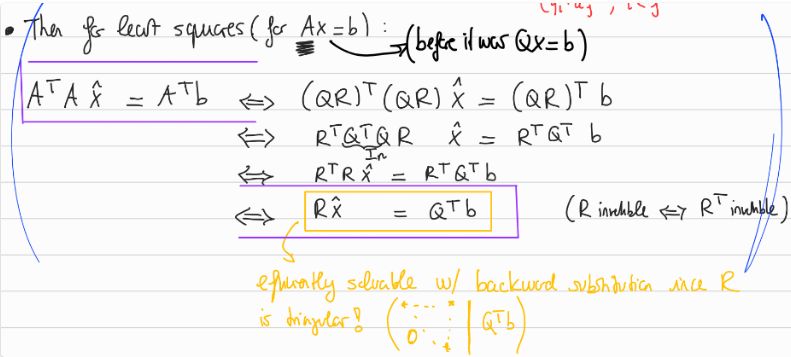
Current
Note has been deleted
Field-by-field Comparison
| Field | Before | After |
|---|---|---|
| Front | ||
| Back |
Note 1385: ETH::1. Semester::LinAlg
Deck: ETH::1. Semester::LinAlg
Note Type: Horvath Cloze
GUID:
deleted
Note Type: Horvath Cloze
GUID:
jGly4b:5@T
Deleted Note
Front
Let \(T :V \rightarrow W\) be a bijective linear transformation between vector spaces \(V\) and \(W\) . Let \(B = {v1, v2, . . . , v_l} \subseteq V\) be a finite set of size \(l\), and let \[ T(B) = {T(v_1), T(v_2), \dots, T(v_l)} \subseteq Q \] be the transformed set.
Then \(|T(B)| = |B|\). Moreover, \(B\) is a basis of \(V\) if and only if \(T(B)\) is a basis of \(W\). We therefore also have \(\dim(V) = \dim(W)\).
Back
Let \(T :V \rightarrow W\) be a bijective linear transformation between vector spaces \(V\) and \(W\) . Let \(B = {v1, v2, . . . , v_l} \subseteq V\) be a finite set of size \(l\), and let \[ T(B) = {T(v_1), T(v_2), \dots, T(v_l)} \subseteq Q \] be the transformed set.
Then \(|T(B)| = |B|\). Moreover, \(B\) is a basis of \(V\) if and only if \(T(B)\) is a basis of \(W\). We therefore also have \(\dim(V) = \dim(W)\).
This holds because of the bijectivity of the linear transformation.
Further, if there is one such bijective transformation, then we call the vector spaces isomorphic and \(T\) an isomorphism between \(V\) and \(W\) (Definition 4.28).
Further, if there is one such bijective transformation, then we call the vector spaces isomorphic and \(T\) an isomorphism between \(V\) and \(W\) (Definition 4.28).
Current
Note has been deleted
Field-by-field Comparison
| Field | Before | After |
|---|---|---|
| Text | ||
| Extra |
Note 1386: ETH::1. Semester::LinAlg
Deck: ETH::1. Semester::LinAlg
Note Type: Horvath Cloze
GUID:
deleted
Note Type: Horvath Cloze
GUID:
je3$vwu2Z6
Deleted Note
Front
Subspaces are orthogonal if their basis-vectors are orthogonal.
Back
Subspaces are orthogonal if their basis-vectors are orthogonal.
We can determine if two subspaces are orthogonal by only comparing their basis vectors, since if they are orthogonal, all their linear combinations will be as well.
Current
Note has been deleted
Field-by-field Comparison
| Field | Before | After |
|---|---|---|
| Text | ||
| Extra |
Note 1387: ETH::1. Semester::LinAlg
Deck: ETH::1. Semester::LinAlg
Note Type: Horvath Cloze
GUID:
deleted
Note Type: Horvath Cloze
GUID:
jfWTLC-Hb%
Deleted Note
Front
Multilinearity of the determinant:\[ \begin{vmatrix} ta & tb \\ c & d \end{vmatrix} = {{c1:: t \cdot \begin{vmatrix} a & b \\ c & d \end{vmatrix} }}\]
Back
Multilinearity of the determinant:\[ \begin{vmatrix} ta & tb \\ c & d \end{vmatrix} = {{c1:: t \cdot \begin{vmatrix} a & b \\ c & d \end{vmatrix} }}\]
Current
Note has been deleted
Field-by-field Comparison
| Field | Before | After |
|---|---|---|
| Text |
Note 1388: ETH::1. Semester::LinAlg
Deck: ETH::1. Semester::LinAlg
Note Type: Horvath Cloze
GUID:
deleted
Note Type: Horvath Cloze
GUID:
jn6
Deleted Note
Front
Let \(A \in \mathbb{R}^{n \times n}\) be a symmetric matrix and \(\lambda_1,\lambda_2 \in \mathbb{R}\) be two distinct eigenvalues of \(A\) with corresponding eigenvectors \(v_1, v_2\):
\(v_1\) and \(v_2\) are orthogonal. Proof Included
Back
Let \(A \in \mathbb{R}^{n \times n}\) be a symmetric matrix and \(\lambda_1,\lambda_2 \in \mathbb{R}\) be two distinct eigenvalues of \(A\) with corresponding eigenvectors \(v_1, v_2\):
\(v_1\) and \(v_2\) are orthogonal. Proof Included
Proof \(\lambda_1 v_1 ^\top v_2 = (Av_1)^\top v_2 = v_1^\top A ^\top v_2 = v_1^\top (Av_2) = \lambda_2 v_1^\top v_2\) Thus \(v_1^\top v_2\) must be \(0\).
Current
Note has been deleted
Field-by-field Comparison
| Field | Before | After |
|---|---|---|
| Text | ||
| Extra |
Note 1389: ETH::1. Semester::LinAlg
Deck: ETH::1. Semester::LinAlg
Note Type: Horvath Cloze
GUID:
deleted
Note Type: Horvath Cloze
GUID:
jo;...VEEI
Deleted Note
Front
A matrix has a complete set of real eigenvectors if all its eigenvalues are real and the geometric multiplicities are the same as the algebraic multiplicities of all it's eigenvalues.
Back
A matrix has a complete set of real eigenvectors if all its eigenvalues are real and the geometric multiplicities are the same as the algebraic multiplicities of all it's eigenvalues.
Example \(I\) has eigenvalue \(1\) with geometric multiplicity \(n\) (\(\dim(N(I - 1 \cdot I)) = n\)) and algebraic multiplicity \(n\) (As the characteristic polynomial of \(I\), \(P(z) = (z - 1)(z - 1) \dots (z - 1)\) with that repeated \(n\) times).
Current
Note has been deleted
Field-by-field Comparison
| Field | Before | After |
|---|---|---|
| Text | ||
| Extra |
Note 1390: ETH::1. Semester::LinAlg
Deck: ETH::1. Semester::LinAlg
Note Type: Horvath Cloze
GUID:
deleted
Note Type: Horvath Cloze
GUID:
ju
Deleted Note
Front
Let \(Q\) be the \(m \times n\) matrix whose columns are an orthonormal basis of \(A\).
Then the least squares solution \(Qx = b\) is given by {{c1:: \(\hat{x} = Q^\top b\)}}.
Back
Let \(Q\) be the \(m \times n\) matrix whose columns are an orthonormal basis of \(A\).
Then the least squares solution \(Qx = b\) is given by {{c1:: \(\hat{x} = Q^\top b\)}}.
Current
Note has been deleted
Field-by-field Comparison
| Field | Before | After |
|---|---|---|
| Text |
Note 1391: ETH::1. Semester::LinAlg
Deck: ETH::1. Semester::LinAlg
Note Type: Horvath Cloze
GUID:
deleted
Note Type: Horvath Cloze
GUID:
juIW6&N76+
Deleted Note
Front
For RREF on \(A, I\) we get \(R, M\) with the property that \(R = MA\) and \(M\) invertible.
Back
For RREF on \(A, I\) we get \(R, M\) with the property that \(R = MA\) and \(M\) invertible.
Current
Note has been deleted
Field-by-field Comparison
| Field | Before | After |
|---|---|---|
| Text |
Note 1392: ETH::1. Semester::LinAlg
Deck: ETH::1. Semester::LinAlg
Note Type: Horvath Classic
GUID:
deleted
Note Type: Horvath Classic
GUID:
kDU~f+!zJB
Deleted Note
Front
Certificate of no solutions:
Given \(P = \{x \in \mathbb{R}^n \mid Ax = b \}\) we have:
\(P = \left\{ x \in \mathbb{R}^3 \;\middle|\; \begin{aligned} x_1 + 2x_2 - x_3 &= 1 \\ 2x_1 + 4x_2 - 2x_3 &= 0 \end{aligned} \right\}\)
Provide the system \(D\) and the answer.
Given \(P = \{x \in \mathbb{R}^n \mid Ax = b \}\) we have:
\(P = \left\{ x \in \mathbb{R}^3 \;\middle|\; \begin{aligned} x_1 + 2x_2 - x_3 &= 1 \\ 2x_1 + 4x_2 - 2x_3 &= 0 \end{aligned} \right\}\)
Provide the system \(D\) and the answer.
Back
Certificate of no solutions:
Given \(P = \{x \in \mathbb{R}^n \mid Ax = b \}\) we have:
\(P = \left\{ x \in \mathbb{R}^3 \;\middle|\; \begin{aligned} x_1 + 2x_2 - x_3 &= 1 \\ 2x_1 + 4x_2 - 2x_3 &= 0 \end{aligned} \right\}\)
Provide the system \(D\) and the answer.
Given \(P = \{x \in \mathbb{R}^n \mid Ax = b \}\) we have:
\(P = \left\{ x \in \mathbb{R}^3 \;\middle|\; \begin{aligned} x_1 + 2x_2 - x_3 &= 1 \\ 2x_1 + 4x_2 - 2x_3 &= 0 \end{aligned} \right\}\)
Provide the system \(D\) and the answer.
The system \(D = \{ z \in \mathbb{R}^m | A^\top z = 0, b^\top z = 1 \}\) then is: \[D = \left\{ z \in \mathbb{R}^2 \;\middle|\; \begin{aligned} z_1 + 2z_2 &= 0 \\ 2z_1 + 4z_2 &= 0 \\ -z_1 - 2z_2 &= 0 \\ z_1 &= 1 \end{aligned} \right\}\]One equation per each column of \(A\).
\(P = \emptyset\) and \(D \neq \emptyset\) because \(z = (1, -\frac{1}{2})^\top \in D\).
\(P = \emptyset\) and \(D \neq \emptyset\) because \(z = (1, -\frac{1}{2})^\top \in D\).
Current
Note has been deleted
Field-by-field Comparison
| Field | Before | After |
|---|---|---|
| Front | ||
| Back |
Note 1393: ETH::1. Semester::LinAlg
Deck: ETH::1. Semester::LinAlg
Note Type: Horvath Classic
GUID:
deleted
Note Type: Horvath Classic
GUID:
kRJ}a-S?@*
Deleted Note
Front
Formula for the cosine of the angle between vectors v and w
Back
Formula for the cosine of the angle between vectors v and w
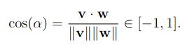
If v and w are unit vectors, we don't need to divide by their norms, see the definition of a scalar product geometrically.
Current
Note has been deleted
Field-by-field Comparison
| Field | Before | After |
|---|---|---|
| Front | ||
| Back |
Note 1394: ETH::1. Semester::LinAlg
Deck: ETH::1. Semester::LinAlg
Note Type: Horvath Classic
GUID:
deleted
Note Type: Horvath Classic
GUID:
kUcA5;!CKY
Deleted Note
Front
Give an example of a matrix with complex valued EWs:
Back
Give an example of a matrix with complex valued EWs:
Eigenvalues of the \(90^\circ\) degree counterclockwise rotation matrix \(A = \begin{bmatrix} 0 & -1 \\ 1 & 0 \end{bmatrix}\).
The solutions to \(0 = \det(A - \lambda I) = -\lambda \cdot -\lambda - 1 \cdot (-1) = \lambda^2 + 1\) which are \(\lambda_1 = i\) and \(\lambda_2 = -i\). The eigenvectors are given by \(v_1 = \begin{pmatrix} i \\ 1 \end{pmatrix}\) \(v_2 = \begin{pmatrix} -i \\ 1 \end{pmatrix}\).
This makes sense because the only vector staying on it's axis in a 2d rotation of a plane by \(90^\circ\) is the vector pointing straight up, out from the plane.
Current
Note has been deleted
Field-by-field Comparison
| Field | Before | After |
|---|---|---|
| Front | ||
| Back |
Note 1395: ETH::1. Semester::LinAlg
Deck: ETH::1. Semester::LinAlg
Note Type: Horvath Cloze
GUID:
deleted
Note Type: Horvath Cloze
GUID:
k_E{8UgRT{
Deleted Note
Front
The dimensions of a hyperplane \(H\) through the origin in \(\mathbb{R}^m\) is \(m - 1\).
Back
The dimensions of a hyperplane \(H\) through the origin in \(\mathbb{R}^m\) is \(m - 1\).
See assignment 6 proof.
Current
Note has been deleted
Field-by-field Comparison
| Field | Before | After |
|---|---|---|
| Text | ||
| Extra |
Note 1396: ETH::1. Semester::LinAlg
Deck: ETH::1. Semester::LinAlg
Note Type: Horvath Cloze
GUID:
deleted
Note Type: Horvath Cloze
GUID:
krdY1rh*f]
Deleted Note
Front
If \(AB = BA\) then they share an EV and thus \(A + B\) also has that EV.
Back
If \(AB = BA\) then they share an EV and thus \(A + B\) also has that EV.
If both \(A\) and \(B\) share an EV:
\((A + B)v = Av + Bv = \lambda v + \lambda' v = (\lambda + \lambda')v\) then \(A + B\) also has that EV.
\((A + B)v = Av + Bv = \lambda v + \lambda' v = (\lambda + \lambda')v\) then \(A + B\) also has that EV.
Current
Note has been deleted
Field-by-field Comparison
| Field | Before | After |
|---|---|---|
| Text | ||
| Extra |
Note 1397: ETH::1. Semester::LinAlg
Deck: ETH::1. Semester::LinAlg
Note Type: Horvath Classic
GUID:
deleted
Note Type: Horvath Classic
GUID:
ku_5}q!4@#
Deleted Note
Front
A linear combination of \(\lambda_1\textbf{v}_1 + \lambda_2\textbf{v}_2 + \dots + \lambda_n\textbf{v}_n\) is affine if
Back
A linear combination of \(\lambda_1\textbf{v}_1 + \lambda_2\textbf{v}_2 + \dots + \lambda_n\textbf{v}_n\) is affine if
\(\lambda_1 + \lambda_2 + \dots + \lambda_n = 1\)
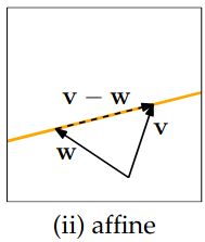
Current
Note has been deleted
Field-by-field Comparison
| Field | Before | After |
|---|---|---|
| Front | ||
| Back |
Note 1398: ETH::1. Semester::LinAlg
Deck: ETH::1. Semester::LinAlg
Note Type: Horvath Cloze
GUID:
deleted
Note Type: Horvath Cloze
GUID:
l4%P|7pgCb
Deleted Note
Front
What are the four Moore-Penrose conditions?
- \(AA^\dagger A = A\)
- \(A^\dagger A A^\dagger = A^\dagger\)
- \((AA^\dagger )^\top = AA^\dagger \)
- \((A^\dagger A)^\top = A^\dagger A\)
Back
What are the four Moore-Penrose conditions?
- \(AA^\dagger A = A\)
- \(A^\dagger A A^\dagger = A^\dagger\)
- \((AA^\dagger )^\top = AA^\dagger \)
- \((A^\dagger A)^\top = A^\dagger A\)
Current
Note has been deleted
Field-by-field Comparison
| Field | Before | After |
|---|---|---|
| Text |
Note 1399: ETH::1. Semester::LinAlg
Deck: ETH::1. Semester::LinAlg
Note Type: Horvath Classic
GUID:
deleted
Note Type: Horvath Classic
GUID:
l
Deleted Note
Front
How do we solve \(Ax = b\) using RREF?
Back
How do we solve \(Ax = b\) using RREF?
We run \(\text{RREF}(A, b)\) and solve the resulting equation using back-substitution.
Current
Note has been deleted
Field-by-field Comparison
| Field | Before | After |
|---|---|---|
| Front | ||
| Back |
Note 1400: ETH::1. Semester::LinAlg
Deck: ETH::1. Semester::LinAlg
Note Type: Horvath Cloze
GUID:
deleted
Note Type: Horvath Cloze
GUID:
l?,e(>h5cQ
Deleted Note
Front
We say that \(A \in \mathbb{R}^{n \times n}\) and \(B \in \mathbb{R}^{n \times n}\) are similar matrices if {{c2::there exists an invertible matrix \(S\) such that \(B = S^{-1}AS\)}}.
Back
We say that \(A \in \mathbb{R}^{n \times n}\) and \(B \in \mathbb{R}^{n \times n}\) are similar matrices if {{c2::there exists an invertible matrix \(S\) such that \(B = S^{-1}AS\)}}.
Current
Note has been deleted
Field-by-field Comparison
| Field | Before | After |
|---|---|---|
| Text |
Note 1401: ETH::1. Semester::LinAlg
Deck: ETH::1. Semester::LinAlg
Note Type: Horvath Cloze
GUID:
deleted
Note Type: Horvath Cloze
GUID:
l@6E)FW9<^
Deleted Note
Front
Let \(A \in \mathbb{R}^{n \times n}\) and \(\lambda_1, \dots, \lambda_n\) its \(n\) eigenvalues. Then \[ \text{Tr}(A) = {{c1:: \sum_{i = 1}^n \lambda_i :: \text{in terms of EWs} }}\]
Back
Let \(A \in \mathbb{R}^{n \times n}\) and \(\lambda_1, \dots, \lambda_n\) its \(n\) eigenvalues. Then \[ \text{Tr}(A) = {{c1:: \sum_{i = 1}^n \lambda_i :: \text{in terms of EWs} }}\]
Quite surprising, since the determinant and trace are \(\in \mathbb{R}\) where the eigenvalues in general must not be?
It holds because complex eigenvalues \(z_1, z_2\) always show up in pairs: \(z_1 = \overline{z_2}\). And because \(z_1 \cdot \overline{z_1} = a^2 + b^2\) and \(z_1 + \overline{z_1} = 2a\).
It holds because complex eigenvalues \(z_1, z_2\) always show up in pairs: \(z_1 = \overline{z_2}\). And because \(z_1 \cdot \overline{z_1} = a^2 + b^2\) and \(z_1 + \overline{z_1} = 2a\).
Current
Note has been deleted
Field-by-field Comparison
| Field | Before | After |
|---|---|---|
| Text | ||
| Extra |
Note 1402: ETH::1. Semester::LinAlg
Deck: ETH::1. Semester::LinAlg
Note Type: Horvath Classic
GUID:
deleted
Note Type: Horvath Classic
GUID:
lG3L]2Sq+d
Deleted Note
Front
Was ist der Rang eines LGS?
Back
Was ist der Rang eines LGS?
Die Anzahl Pivotelemente bzw. die Anzahl Zeilen, welche nicht Nullzeilen sind.
Current
Note has been deleted
Field-by-field Comparison
| Field | Before | After |
|---|---|---|
| Front | ||
| Back |
Note 1403: ETH::1. Semester::LinAlg
Deck: ETH::1. Semester::LinAlg
Note Type: Horvath Classic
GUID:
deleted
Note Type: Horvath Classic
GUID:
lK,rOhy|Tw
Deleted Note
Front
If we have \(A\) with eigenvalues \(0, 1, 2\) then \(I + A^2\) has eigenvalues?
Back
If we have \(A\) with eigenvalues \(0, 1, 2\) then \(I + A^2\) has eigenvalues?
We have \(\lambda^2\) eigenvalues of \(A^2\) by lemma script. Thus \(0, 1, 4\) are EWs.
Then \(1 + \lambda^2\) are the eigenvalues of \(I + A^2\) thus \(1, 2, 5\) are the EWs.
Then \(1 + \lambda^2\) are the eigenvalues of \(I + A^2\) thus \(1, 2, 5\) are the EWs.
Current
Note has been deleted
Field-by-field Comparison
| Field | Before | After |
|---|---|---|
| Front | ||
| Back |
Note 1404: ETH::1. Semester::LinAlg
Deck: ETH::1. Semester::LinAlg
Note Type: Horvath Cloze
GUID:
deleted
Note Type: Horvath Cloze
GUID:
lO6]X2n6eN
Deleted Note
Front
Let \(A\) be an \(m \times m\) invertible matrix.
Then the transpose \(A^T\) is also invertible and: \( (A^T)^{-1} = \) {{c1:: \((A^{-1})^T \)}}
Then the transpose \(A^T\) is also invertible and: \( (A^T)^{-1} = \) {{c1:: \((A^{-1})^T \)}}
Back
Let \(A\) be an \(m \times m\) invertible matrix.
Then the transpose \(A^T\) is also invertible and: \( (A^T)^{-1} = \) {{c1:: \((A^{-1})^T \)}}
Then the transpose \(A^T\) is also invertible and: \( (A^T)^{-1} = \) {{c1:: \((A^{-1})^T \)}}
Current
Note has been deleted
Field-by-field Comparison
| Field | Before | After |
|---|---|---|
| Text |
Note 1405: ETH::1. Semester::LinAlg
Deck: ETH::1. Semester::LinAlg
Note Type: Horvath Classic
GUID:
deleted
Note Type: Horvath Classic
GUID:
lZ8TNAe;8y
Deleted Note
Front
How do we get from \(\det(A - zI)\) to \(\det(zI - A)\)?
Back
How do we get from \(\det(A - zI)\) to \(\det(zI - A)\)?
We can transform \(\det(A - zI) =\) \((-1)^n \det((-1)(A - zI))\) \(= (-1)^n \det(zI - A)\) because \(\det(\lambda A) = \lambda^n \det(A)\).
Current
Note has been deleted
Field-by-field Comparison
| Field | Before | After |
|---|---|---|
| Front | ||
| Back |
Note 1406: ETH::1. Semester::LinAlg
Deck: ETH::1. Semester::LinAlg
Note Type: Horvath Classic
GUID:
deleted
Note Type: Horvath Classic
GUID:
l[e7/3<
Deleted Note
Front
If columns \(v_1, v_2, ..., v_n\) of \(A\) are linearly independent and \(A\lambda = A\mu = x\) are two ways of writing vector x as a linear combination of the vectors v then:
Back
If columns \(v_1, v_2, ..., v_n\) of \(A\) are linearly independent and \(A\lambda = A\mu = x\) are two ways of writing vector x as a linear combination of the vectors v then:
\(\lambda \ \text{and} \ \mu\) are the exact same vector of coefficients.
Linear combinations are unique if all vectors are independent.
Current
Note has been deleted
Field-by-field Comparison
| Field | Before | After |
|---|---|---|
| Front | ||
| Back |
Note 1407: ETH::1. Semester::LinAlg
Deck: ETH::1. Semester::LinAlg
Note Type: Horvath Cloze
GUID:
deleted
Note Type: Horvath Cloze
GUID:
l_;^0p%n!C
Deleted Note
Front
Every matrix transformation is a linear transformation.
Back
Every matrix transformation is a linear transformation.
The inverse is also true.
Current
Note has been deleted
Field-by-field Comparison
| Field | Before | After |
|---|---|---|
| Text | ||
| Extra |
Note 1408: ETH::1. Semester::LinAlg
Deck: ETH::1. Semester::LinAlg
Note Type: Horvath Classic
GUID:
deleted
Note Type: Horvath Classic
GUID:
lgnIL]HR}%
Deleted Note
Front
What can we use to speed up long matrix multiplications, for example \(w^\intercal (vw^\intercal) v\)?
Back
What can we use to speed up long matrix multiplications, for example \(w^\intercal (vw^\intercal) v\)?
We can use associativity: \(w^\intercal (vw^\intercal) v = (w^\intercal v)(w^\intercal v)\).
Current
Note has been deleted
Field-by-field Comparison
| Field | Before | After |
|---|---|---|
| Front | ||
| Back |
Note 1409: ETH::1. Semester::LinAlg
Deck: ETH::1. Semester::LinAlg
Note Type: Horvath Classic
GUID:
deleted
Note Type: Horvath Classic
GUID:
lh.Ty3ypWO
Deleted Note
Front
How do we find a basis for the row space \(R(A) = C(A^\top)\)?
Back
How do we find a basis for the row space \(R(A) = C(A^\top)\)?
The first \(r\) columns of \(R^\top\) where \(R\) is the RREF of \(A\) form a basis of the row space (the non-zero rows). In particular \(\dim(\textbf{R}(A)) = r\)
This works because as noted before, multiplying by an invertible matrix \(M\) does not change the row-space of \(MA\) on the left.
Current
Note has been deleted
Field-by-field Comparison
| Field | Before | After |
|---|---|---|
| Front | ||
| Back |
Note 1410: ETH::1. Semester::LinAlg
Deck: ETH::1. Semester::LinAlg
Note Type: Horvath Classic
GUID:
deleted
Note Type: Horvath Classic
GUID:
ltjw8T1j7K
Deleted Note
Front
The span \(\textbf{Span}(\emptyset)\) is:
Back
The span \(\textbf{Span}(\emptyset)\) is:
\(\{0\}\) only the zero vector, as the empty sum = 0.
Current
Note has been deleted
Field-by-field Comparison
| Field | Before | After |
|---|---|---|
| Front | ||
| Back |
Note 1411: ETH::1. Semester::LinAlg
Deck: ETH::1. Semester::LinAlg
Note Type: Horvath Cloze
GUID:
deleted
Note Type: Horvath Cloze
GUID:
m!}r_v/6N8
Deleted Note
Front
The eigenvalues of \(A\) are the same ones as those of \(A^\top\).
Back
The eigenvalues of \(A\) are the same ones as those of \(A^\top\).
Current
Note has been deleted
Field-by-field Comparison
| Field | Before | After |
|---|---|---|
| Text |
Note 1412: ETH::1. Semester::LinAlg
Deck: ETH::1. Semester::LinAlg
Note Type: Horvath Cloze
GUID:
deleted
Note Type: Horvath Cloze
GUID:
m)DHqZ}2Ss
Deleted Note
Front
Give the three definitions of linear dependence:
- At least one of the vectors is a linear combination of the other ones.
- {{c2::There are scalars \(\lambda_1, ..., \lambda_n\) besides 0, 0, ..., 0 such that \(\sum_{i = 1}^n \lambda_i v_i = \mathbf{0}\). \(\mathbf{0}\) is a nontrivial combination of the vectors.}}
- At least one of the vectors is a linear combination of the previous ones.
Back
Give the three definitions of linear dependence:
- At least one of the vectors is a linear combination of the other ones.
- {{c2::There are scalars \(\lambda_1, ..., \lambda_n\) besides 0, 0, ..., 0 such that \(\sum_{i = 1}^n \lambda_i v_i = \mathbf{0}\). \(\mathbf{0}\) is a nontrivial combination of the vectors.}}
- At least one of the vectors is a linear combination of the previous ones.
Current
Note has been deleted
Field-by-field Comparison
| Field | Before | After |
|---|---|---|
| Text |
Note 1413: ETH::1. Semester::LinAlg
Deck: ETH::1. Semester::LinAlg
Note Type: Horvath Cloze
GUID:
deleted
Note Type: Horvath Cloze
GUID:
m:%R_Tln*C
Deleted Note
Front
Let \(V\) be a subspace of \(\mathbb{R}^n\). Then \(V = (V^\perp)^\perp\)
Back
Let \(V\) be a subspace of \(\mathbb{R}^n\). Then \(V = (V^\perp)^\perp\)
Current
Note has been deleted
Field-by-field Comparison
| Field | Before | After |
|---|---|---|
| Text |
Note 1414: ETH::1. Semester::LinAlg
Deck: ETH::1. Semester::LinAlg
Note Type: Horvath Cloze
GUID:
deleted
Note Type: Horvath Cloze
GUID:
m=XX+5;W*i
Deleted Note
Front
Two subspaces \(V\) and \(W\) are orthogonal if for all \(v \in V\) and \(w \in W\), the vectors \(v\) and \(w\) are orthogonal.
Back
Two subspaces \(V\) and \(W\) are orthogonal if for all \(v \in V\) and \(w \in W\), the vectors \(v\) and \(w\) are orthogonal.
Two vectors \(v, w \in \mathbb{R}^n\) are called orthogonal if \(v^\top w = \sum_{i = 1}^n v_i w_i = 0\).
Current
Note has been deleted
Field-by-field Comparison
| Field | Before | After |
|---|---|---|
| Text | ||
| Extra |
Note 1415: ETH::1. Semester::LinAlg
Deck: ETH::1. Semester::LinAlg
Note Type: Horvath Cloze
GUID:
deleted
Note Type: Horvath Cloze
GUID:
mP8DeYC`=|
Deleted Note
Front
A vector \(v \in \mathbb{R}^n \setminus \{0\}\) is an eigenvector associated with the eigenvalue \(\lambda\) if and only if \(v \in N(A - \lambda I)\).
Back
A vector \(v \in \mathbb{R}^n \setminus \{0\}\) is an eigenvector associated with the eigenvalue \(\lambda\) if and only if \(v \in N(A - \lambda I)\).
Current
Note has been deleted
Field-by-field Comparison
| Field | Before | After |
|---|---|---|
| Text |
Note 1416: ETH::1. Semester::LinAlg
Deck: ETH::1. Semester::LinAlg
Note Type: Horvath Cloze
GUID:
deleted
Note Type: Horvath Cloze
GUID:
mdTBSy$[M4
Deleted Note
Front
Vectors \(q_1, \dots, q_n \in \mathbb{R}^m\) are orthonormal if they are orthogonal and have norm \(1\).
In other words, for all \(i, j \in \{1, \dots, n\}\): \[ q_i^\top q_j = {{c1::\delta_{ij} }}\]
In other words, for all \(i, j \in \{1, \dots, n\}\): \[ q_i^\top q_j = {{c1::\delta_{ij} }}\]
Back
Vectors \(q_1, \dots, q_n \in \mathbb{R}^m\) are orthonormal if they are orthogonal and have norm \(1\).
In other words, for all \(i, j \in \{1, \dots, n\}\): \[ q_i^\top q_j = {{c1::\delta_{ij} }}\]
In other words, for all \(i, j \in \{1, \dots, n\}\): \[ q_i^\top q_j = {{c1::\delta_{ij} }}\]
Current
Note has been deleted
Field-by-field Comparison
| Field | Before | After |
|---|---|---|
| Text |
Note 1417: ETH::1. Semester::LinAlg
Deck: ETH::1. Semester::LinAlg
Note Type: Horvath Classic
GUID:
deleted
Note Type: Horvath Classic
GUID:
moUy5DUi0d
Deleted Note
Front
What is the definition of a hyperplane?
Back
What is the definition of a hyperplane?
given a vector \(\mathbf{d} \in \mathbb{R}^n\) \(\mathbf{d} \neq \mathbf{0}\), \(H_{\mathbf{d}} = \{\mathbf{v} \in \mathbb{R}^n : \mathbf{v} \cdot \mathbf{d} = \mathbf{0} \}\)
or in other words, it is the set of vectors orthogonal to a given vector
Since 0 is orthogonal to every vector \(0 \in H_d\).
or in other words, it is the set of vectors orthogonal to a given vector
Since 0 is orthogonal to every vector \(0 \in H_d\).
Current
Note has been deleted
Field-by-field Comparison
| Field | Before | After |
|---|---|---|
| Front | ||
| Back |
Note 1418: ETH::1. Semester::LinAlg
Deck: ETH::1. Semester::LinAlg
Note Type: Horvath Cloze
GUID:
deleted
Note Type: Horvath Cloze
GUID:
mqSXu9R3oO
Deleted Note
Front
The LU (Lower-Upper, also sometimes called LR) decomposition factors a matrix \(A\) as the product of a lower triangular matrix \(L\) and an upper triangular matrix \(U\).
Back
The LU (Lower-Upper, also sometimes called LR) decomposition factors a matrix \(A\) as the product of a lower triangular matrix \(L\) and an upper triangular matrix \(U\).
(so \(A = LU\))
Current
Note has been deleted
Field-by-field Comparison
| Field | Before | After |
|---|---|---|
| Text | ||
| Extra |
Note 1419: ETH::1. Semester::LinAlg
Deck: ETH::1. Semester::LinAlg
Note Type: Horvath Cloze
GUID:
deleted
Note Type: Horvath Cloze
GUID:
n.vpbl!(Kk
Deleted Note
Front
For \(A \in \mathbb{R}^{m \times n}\) with \(\text{rank}(A) = r\), let {{c1:: \(S \in \mathbb{R}^{m \times r}\) and \(T \in \mathbb{R}^{r \times n}\)}} such that \(A = ST\). Then \[ A^\dagger = T^\dagger S^\dagger \]
Back
For \(A \in \mathbb{R}^{m \times n}\) with \(\text{rank}(A) = r\), let {{c1:: \(S \in \mathbb{R}^{m \times r}\) and \(T \in \mathbb{R}^{r \times n}\)}} such that \(A = ST\). Then \[ A^\dagger = T^\dagger S^\dagger \]
Current
Note has been deleted
Field-by-field Comparison
| Field | Before | After |
|---|---|---|
| Text |
Note 1420: ETH::1. Semester::LinAlg
Deck: ETH::1. Semester::LinAlg
Note Type: Horvath Classic
GUID:
deleted
Note Type: Horvath Classic
GUID:
n060vly>1q
Deleted Note
Front
The Cauchy-Schwarz Inequality tells us that for \(\textbf{v}, \textbf{w} \in \mathbb{R}^m\)
Back
The Cauchy-Schwarz Inequality tells us that for \(\textbf{v}, \textbf{w} \in \mathbb{R}^m\)
\(|\textbf{v} \cdot \textbf{w}| \leq ||\textbf{v}|| \ ||\textbf{w}||\).
This equality holds exactly if one vector is the scalar multiple of the other.
This essentially means that: the length of the projecton of v onto w is smaller than the both of their lengths multiplied.
This explains the equality part: if they are already aligned, their projection doesn't lose any length...
Current
Note has been deleted
Field-by-field Comparison
| Field | Before | After |
|---|---|---|
| Front | ||
| Back |
Note 1421: ETH::1. Semester::LinAlg
Deck: ETH::1. Semester::LinAlg
Note Type: Horvath Cloze
GUID:
deleted
Note Type: Horvath Cloze
GUID:
n6JsTlECEy
Deleted Note
Front
Let \(V\) and \(W\) be orthogonal subspaces. If \(\dim(V) = k\) and \(\dim(W) = l\), then:
\(\dim(V + W) = k + l \leq n\).
Back
Let \(V\) and \(W\) be orthogonal subspaces. If \(\dim(V) = k\) and \(\dim(W) = l\), then:
\(\dim(V + W) = k + l \leq n\).
\(\dim(V + W) = \dim(V)+\dim(W)- \dim(V∩W) \)
Current
Note has been deleted
Field-by-field Comparison
| Field | Before | After |
|---|---|---|
| Text | ||
| Extra |
Note 1422: ETH::1. Semester::LinAlg
Deck: ETH::1. Semester::LinAlg
Note Type: Horvath Classic
GUID:
deleted
Note Type: Horvath Classic
GUID:
nCym|+n@l+
Deleted Note
Front
We can view the matrix-vector product \(Ax\) in two ways:
Back
We can view the matrix-vector product \(Ax\) in two ways:
- Row view: The result is a vector where each entry is the scalar product of row \(i\) of \(A\) with \(x\): \((Ax)_{i} = A_i^\top x\).
- Column view: The resulting vector is a linear combination of the columns of \(A\).
Current
Note has been deleted
Field-by-field Comparison
| Field | Before | After |
|---|---|---|
| Front | ||
| Back |
Note 1423: ETH::1. Semester::LinAlg
Deck: ETH::1. Semester::LinAlg
Note Type: Horvath Cloze
GUID:
deleted
Note Type: Horvath Cloze
GUID:
nECE)EKh&n
Deleted Note
Front
When solving Least Squares (asking for a minimiser of \(||Ax - b||^2\)) we are asking \(Ax\) to be the projection of \(b\) onto \(C(A)\).
Back
When solving Least Squares (asking for a minimiser of \(||Ax - b||^2\)) we are asking \(Ax\) to be the projection of \(b\) onto \(C(A)\).
Least Squares is basically projection without multiplying by \(A\) at the end.
It's also basically the Pseudoinverse.
It's also basically the Pseudoinverse.
Current
Note has been deleted
Field-by-field Comparison
| Field | Before | After |
|---|---|---|
| Text | ||
| Extra |
Note 1424: ETH::1. Semester::LinAlg
Deck: ETH::1. Semester::LinAlg
Note Type: Horvath Cloze
GUID:
deleted
Note Type: Horvath Cloze
GUID:
ng]r$T$54^
Deleted Note
Front
By multilinearity, \(\det(\alpha A) = \) \(\alpha^n \det(A)\) Intuition included
Back
By multilinearity, \(\det(\alpha A) = \) \(\alpha^n \det(A)\) Intuition included
the scaling affects all rows equally, thus the unit cube is scaled in all dimensions (power of n).
In other words, we have to extract \(\alpha\) from each row using multilinearity.
In other words, we have to extract \(\alpha\) from each row using multilinearity.
Current
Note has been deleted
Field-by-field Comparison
| Field | Before | After |
|---|---|---|
| Text | ||
| Extra |
Note 1425: ETH::1. Semester::LinAlg
Deck: ETH::1. Semester::LinAlg
Note Type: Horvath Cloze
GUID:
deleted
Note Type: Horvath Cloze
GUID:
nkL&a6|Q;d
Deleted Note
Front
The span of m linearly independent vectors is {{c1::\(\mathbb{R}^m\)}}.
Back
The span of m linearly independent vectors is {{c1::\(\mathbb{R}^m\)}}.
This also means that a matrix in \(\mathbb{R}^{n \times n}\) with rank(A) = n spans the entire space.
Current
Note has been deleted
Field-by-field Comparison
| Field | Before | After |
|---|---|---|
| Text | ||
| Extra |
Note 1426: ETH::1. Semester::LinAlg
Deck: ETH::1. Semester::LinAlg
Note Type: Horvath Classic
GUID:
deleted
Note Type: Horvath Classic
GUID:
nkw:=NZ1ua
Deleted Note
Front
The scalar product of \(\textbf{v} \cdot \textbf{v}\) is \(\leq or \geq\) to what?
Back
The scalar product of \(\textbf{v} \cdot \textbf{v}\) is \(\leq or \geq\) to what?
\(\textbf{v} \cdot \textbf{v} \geq 0\) with equality exactly if \(\textbf{v} = \textbf{0}\).
This is because we essentially square the entries and thus can't get negatives.
This is because we essentially square the entries and thus can't get negatives.
Current
Note has been deleted
Field-by-field Comparison
| Field | Before | After |
|---|---|---|
| Front | ||
| Back |
Note 1427: ETH::1. Semester::LinAlg
Deck: ETH::1. Semester::LinAlg
Note Type: Horvath Cloze
GUID:
deleted
Note Type: Horvath Cloze
GUID:
nte!7ERw=M
Deleted Note
Front
Gram-Schmidt Algorithm:
- {{c2::Normalise \(a_1\) to get \(q_1 = \frac{a_1}{||a_1||}\)}}.
- For \(k = 2, \dots, n\) set {{c1:: \[\begin{align*} q'_k =& a_k - \sum_{i = 1}^{k - 1} (a_k^\top q_i)q_i \\ q_k =& \frac{q_k'}{||q'_k} \end{align*}\]}}
Back
Gram-Schmidt Algorithm:
- {{c2::Normalise \(a_1\) to get \(q_1 = \frac{a_1}{||a_1||}\)}}.
- For \(k = 2, \dots, n\) set {{c1:: \[\begin{align*} q'_k =& a_k - \sum_{i = 1}^{k - 1} (a_k^\top q_i)q_i \\ q_k =& \frac{q_k'}{||q'_k} \end{align*}\]}}
Current
Note has been deleted
Field-by-field Comparison
| Field | Before | After |
|---|---|---|
| Text |
Note 1428: ETH::1. Semester::LinAlg
Deck: ETH::1. Semester::LinAlg
Note Type: Horvath Cloze
GUID:
deleted
Note Type: Horvath Cloze
GUID:
o!YxXMzDp4
Deleted Note
Front
For \(A\) and \(MA\) (\(M\) invertible) they have:
- the independent columns at the same indices
- the same rank
Back
For \(A\) and \(MA\) (\(M\) invertible) they have:
- the independent columns at the same indices
- the same rank
Current
Note has been deleted
Field-by-field Comparison
| Field | Before | After |
|---|---|---|
| Text |
Note 1429: ETH::1. Semester::LinAlg
Deck: ETH::1. Semester::LinAlg
Note Type: Horvath Cloze
GUID:
deleted
Note Type: Horvath Cloze
GUID:
o#.FGP:Yyu
Deleted Note
Front
An EW can have many EVs associated with it.
Back
An EW can have many EVs associated with it.
Current
Note has been deleted
Field-by-field Comparison
| Field | Before | After |
|---|---|---|
| Text |
Note 1430: ETH::1. Semester::LinAlg
Deck: ETH::1. Semester::LinAlg
Note Type: Horvath Cloze
GUID:
deleted
Note Type: Horvath Cloze
GUID:
o1l!C8m&a8
Deleted Note
Front
Theorem: A matrix \(A \in \mathbb{R}^{m \times n}\) of rank \(r\) can be written as the matrix-matrix product \[ A = C R’ \] where \(C\) is the \(m \times r\) submatrix containing the independent columns and the unique \(R’ \in \mathbb{R}^{r \times n}\) matrix.
Back
Theorem: A matrix \(A \in \mathbb{R}^{m \times n}\) of rank \(r\) can be written as the matrix-matrix product \[ A = C R’ \] where \(C\) is the \(m \times r\) submatrix containing the independent columns and the unique \(R’ \in \mathbb{R}^{r \times n}\) matrix.
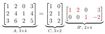
Current
Note has been deleted
Field-by-field Comparison
| Field | Before | After |
|---|---|---|
| Text | ||
| Extra |
Note 1431: ETH::1. Semester::LinAlg
Deck: ETH::1. Semester::LinAlg
Note Type: Horvath Classic
GUID:
deleted
Note Type: Horvath Classic
GUID:
o43^1:-/Cw
Deleted Note
Front
What is the rank of a matrix?
Back
What is the rank of a matrix?
it is the number of independent columns, where independence is defined such that given a column vector \(v_j\) then \(v_j\) is not a linear combination of \(v_1, v_2 ... v_{j-1}\)
Current
Note has been deleted
Field-by-field Comparison
| Field | Before | After |
|---|---|---|
| Front | ||
| Back |
Note 1432: ETH::1. Semester::LinAlg
Deck: ETH::1. Semester::LinAlg
Note Type: Horvath Classic
GUID:
deleted
Note Type: Horvath Classic
GUID:
o5s2_Ks)ET
Deleted Note
Front
Give an example of a non-finitely generated vector space:
Back
Give an example of a non-finitely generated vector space:
\(\mathbb{R}[x]\) is not finitely generated for example.
Current
Note has been deleted
Field-by-field Comparison
| Field | Before | After |
|---|---|---|
| Front | ||
| Back |
Note 1433: ETH::1. Semester::LinAlg
Deck: ETH::1. Semester::LinAlg
Note Type: Horvath Cloze
GUID:
deleted
Note Type: Horvath Cloze
GUID:
o:UCmI*%e|
Deleted Note
Front
Let \(A \in \mathbb{R}^{n \times n}\).
\(\lambda \in \mathbb{R}\) is a real eigenvalue of \(A\) if and only if \(\det(A - \lambda I) = 0\).
Back
Let \(A \in \mathbb{R}^{n \times n}\).
\(\lambda \in \mathbb{R}\) is a real eigenvalue of \(A\) if and only if \(\det(A - \lambda I) = 0\).
Current
Note has been deleted
Field-by-field Comparison
| Field | Before | After |
|---|---|---|
| Text |
Note 1434: ETH::1. Semester::LinAlg
Deck: ETH::1. Semester::LinAlg
Note Type: Horvath Cloze
GUID:
deleted
Note Type: Horvath Cloze
GUID:
oKlE5w/*RH
Deleted Note
Front
If \(Q \in \mathbb{R}^{n \times n}\) is an orthogonal matrix then \(\det(Q) = \) \(1\) or \(-1\).
Back
If \(Q \in \mathbb{R}^{n \times n}\) is an orthogonal matrix then \(\det(Q) = \) \(1\) or \(-1\).
As \(Q\) is orthogonal, we don't scale (preserves \(\top\)) thus the unit cube is just turned, not scaled.
Current
Note has been deleted
Field-by-field Comparison
| Field | Before | After |
|---|---|---|
| Text | ||
| Extra |
Note 1435: ETH::1. Semester::LinAlg
Deck: ETH::1. Semester::LinAlg
Note Type: Horvath Cloze
GUID:
deleted
Note Type: Horvath Cloze
GUID:
oNA@igJ,T/
Deleted Note
Front
\(A\) has a complete set of real eigenvectors if {{c2::we can build a basis of \(\mathbb{R}^n\) with the eigenvectors}}.
Back
\(A\) has a complete set of real eigenvectors if {{c2::we can build a basis of \(\mathbb{R}^n\) with the eigenvectors}}.
Current
Note has been deleted
Field-by-field Comparison
| Field | Before | After |
|---|---|---|
| Text |
Note 1436: ETH::1. Semester::LinAlg
Deck: ETH::1. Semester::LinAlg
Note Type: Horvath Cloze
GUID:
deleted
Note Type: Horvath Cloze
GUID:
oSLQnuRv!X
Deleted Note
Front
Every matrix \(A \in \mathbb{R}^{n \times n}\) has an eigenvalue (perhaps complex-valued).
Back
Every matrix \(A \in \mathbb{R}^{n \times n}\) has an eigenvalue (perhaps complex-valued).
Current
Note has been deleted
Field-by-field Comparison
| Field | Before | After |
|---|---|---|
| Text |
Note 1437: ETH::1. Semester::LinAlg
Deck: ETH::1. Semester::LinAlg
Note Type: Horvath Cloze
GUID:
deleted
Note Type: Horvath Cloze
GUID:
oVmXrU@C,D
Deleted Note
Front
The span of a set of vectors is the set of all possible linear combinations of them.
Back
The span of a set of vectors is the set of all possible linear combinations of them.
The span is a linear subspace.
Current
Note has been deleted
Field-by-field Comparison
| Field | Before | After |
|---|---|---|
| Text | ||
| Extra |
Note 1438: ETH::1. Semester::LinAlg
Deck: ETH::1. Semester::LinAlg
Note Type: Horvath Cloze
GUID:
deleted
Note Type: Horvath Cloze
GUID:
oX/3/jm{Ku
Deleted Note
Front
For a full row rank matrix \(A\), the unique solution to\[{{c1:: \min_{x \in \mathbb{R}^n} ||x||^2 \text{ s.t. } Ax = b}}\] is given by the vector \(\hat{x} = A^\dagger b\). This \(\hat{x}\) is in \(C(A^\top)\). Proof Included
Back
For a full row rank matrix \(A\), the unique solution to\[{{c1:: \min_{x \in \mathbb{R}^n} ||x||^2 \text{ s.t. } Ax = b}}\] is given by the vector \(\hat{x} = A^\dagger b\). This \(\hat{x}\) is in \(C(A^\top)\). Proof Included
Proof
By Lemma 6.4.5 we only need to show that \(\hat{x} = A^\dagger b\) satisfies \(A \hat{x} = b\) and that \(\hat{x} \in C(A^\top)\).
- \(A\hat{x} = AA^\dagger b = AA^\top (AA^\top)^{-1}b = b\)
- \(\hat{x} = A^\dagger b = A^\top ((AA^\top)^{-1} b) = A^\top y\) for some \(y\) thus \(x \in C(A^\top)\).
Current
Note has been deleted
Field-by-field Comparison
| Field | Before | After |
|---|---|---|
| Text | ||
| Extra |
Note 1439: ETH::1. Semester::LinAlg
Deck: ETH::1. Semester::LinAlg
Note Type: Horvath Cloze
GUID:
deleted
Note Type: Horvath Cloze
GUID:
oXvW^EH?&l
Deleted Note
Front
An important difference between a field \(F\) and a vector space \(V\) is that multiplication in the field is \(F\times F\mapsto F\), whereas it is \(F\times V\mapsto V\) in the vector space.
Back
An important difference between a field \(F\) and a vector space \(V\) is that multiplication in the field is \(F\times F\mapsto F\), whereas it is \(F\times V\mapsto V\) in the vector space.
Current
Note has been deleted
Field-by-field Comparison
| Field | Before | After |
|---|---|---|
| Text |
Note 1440: ETH::1. Semester::LinAlg
Deck: ETH::1. Semester::LinAlg
Note Type: Horvath Cloze
GUID:
deleted
Note Type: Horvath Cloze
GUID:
os3Z8p7:x,
Deleted Note
Front
We can compute the pseudoinverse from the any full rank (not just CR) factorisation of \(A\).
Back
We can compute the pseudoinverse from the any full rank (not just CR) factorisation of \(A\).
Note to Lorenz: Leave the "the" in, it's for maximum confusion .
Current
Note has been deleted
Field-by-field Comparison
| Field | Before | After |
|---|---|---|
| Text | ||
| Extra |
Note 1441: ETH::1. Semester::LinAlg
Deck: ETH::1. Semester::LinAlg
Note Type: Horvath Cloze
GUID:
deleted
Note Type: Horvath Cloze
GUID:
p(}O&|&j}p
Deleted Note
Front
The eigenvalues of \(AB\) and \(BA\) are the same.
Back
The eigenvalues of \(AB\) and \(BA\) are the same.
Current
Note has been deleted
Field-by-field Comparison
| Field | Before | After |
|---|---|---|
| Text |
Note 1442: ETH::1. Semester::LinAlg
Deck: ETH::1. Semester::LinAlg
Note Type: Horvath Cloze
GUID:
deleted
Note Type: Horvath Cloze
GUID:
p,i>w2r!)Y
Deleted Note
Front
A matrix \(A\) is nilpotent if {{c1:: there is a \(k \in \mathbb{N}\) such that \(A^k = 0\)}}.
Back
A matrix \(A\) is nilpotent if {{c1:: there is a \(k \in \mathbb{N}\) such that \(A^k = 0\)}}.
In this case, \(A\) cannot have an inverse.
Current
Note has been deleted
Field-by-field Comparison
| Field | Before | After |
|---|---|---|
| Text | ||
| Extra |
Note 1443: ETH::1. Semester::LinAlg
Deck: ETH::1. Semester::LinAlg
Note Type: Horvath Classic
GUID:
deleted
Note Type: Horvath Classic
GUID:
p6e6T6[HIy
Deleted Note
Front
Was ist eine transponierte Matrix?
Back
Was ist eine transponierte Matrix?
Eine entlang der Hauptdiagonale gespiegelte Matrix \(\mathbf{A}^\top\), d.h. \( (\mathbf{A}^\top)_{ij} = (\mathbf{A})_{ji} \)
Current
Note has been deleted
Field-by-field Comparison
| Field | Before | After |
|---|---|---|
| Front | ||
| Back |
Note 1444: ETH::1. Semester::LinAlg
Deck: ETH::1. Semester::LinAlg
Note Type: Horvath Classic
GUID:
deleted
Note Type: Horvath Classic
GUID:
p:TgRlDdKr
Deleted Note
Front
What is the pseudoinverse in the case where \(A \in \mathbb{R}^{n \times m}\) has independent columns?
Back
What is the pseudoinverse in the case where \(A \in \mathbb{R}^{n \times m}\) has independent columns?
Because \(rank(A) = r = n\) and thus \(m \geq n\)
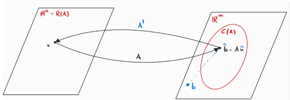
- \(R(A)\) spans \(\mathbb{R}^n\)(rows span the space)
- \(C(A) \subseteq\) \(\mathbb{R}^m\) (as \(A\) is not necessarily square)
We therefore first project \(b\) into \(C(A)\) and then invert, which is Least Squares.
Current
Note has been deleted
Field-by-field Comparison
| Field | Before | After |
|---|---|---|
| Front | ||
| Back |
Note 1445: ETH::1. Semester::LinAlg
Deck: ETH::1. Semester::LinAlg
Note Type: Horvath Cloze
GUID:
deleted
Note Type: Horvath Cloze
GUID:
p>awtIqE5t
Deleted Note
Front
Let \(V\) be a finitely generated vector space.
Then \(\dim(V)\) the dimension of \(V\) is the size of an arbitrary basis \(B\) of \(V\).
Then \(\dim(V)\) the dimension of \(V\) is the size of an arbitrary basis \(B\) of \(V\).
Back
Let \(V\) be a finitely generated vector space.
Then \(\dim(V)\) the dimension of \(V\) is the size of an arbitrary basis \(B\) of \(V\).
Then \(\dim(V)\) the dimension of \(V\) is the size of an arbitrary basis \(B\) of \(V\).
Current
Note has been deleted
Field-by-field Comparison
| Field | Before | After |
|---|---|---|
| Text |
Note 1446: ETH::1. Semester::LinAlg
Deck: ETH::1. Semester::LinAlg
Note Type: Horvath Cloze
GUID:
deleted
Note Type: Horvath Cloze
GUID:
pK()_=6$f)
Deleted Note
Front
Let \(V\) and \(W\) be orthogonal subspaces of \(\mathbb{R}^n\). Let \(v_1, \dots, v_k\) be a basis of subspace \(V\). Let \(w_1, \dots, w_l\) be a basis of subspace \(W\).
The set of vectors \({v_1, \dots, v_k, w_1, \dots, w_l}\) is linearly independent.
Back
Let \(V\) and \(W\) be orthogonal subspaces of \(\mathbb{R}^n\). Let \(v_1, \dots, v_k\) be a basis of subspace \(V\). Let \(w_1, \dots, w_l\) be a basis of subspace \(W\).
The set of vectors \({v_1, \dots, v_k, w_1, \dots, w_l}\) is linearly independent.
As all vectors are pairwise linearly independent, their union is also linearly independent. Therefore the union of two bases is still a basis of the sum of their subspaces:
Current
Note has been deleted
Field-by-field Comparison
| Field | Before | After |
|---|---|---|
| Text | ||
| Extra |
Note 1447: ETH::1. Semester::LinAlg
Deck: ETH::1. Semester::LinAlg
Note Type: Horvath Cloze
GUID:
deleted
Note Type: Horvath Cloze
GUID:
pQ2lENdIXM
Deleted Note
Front
Let \(S^\perp\) be the orthogonal complement of \(S\) and \(P\) the projection matrix onto \(S\).
Then \(I - P\) is the projection matrix that maps {{c2::\(b \in \mathbb{R}^m\) to \(\text{proj}_{S^\perp}(b)\)}}.
Proof Included
Proof Included
Back
Let \(S^\perp\) be the orthogonal complement of \(S\) and \(P\) the projection matrix onto \(S\).
Then \(I - P\) is the projection matrix that maps {{c2::\(b \in \mathbb{R}^m\) to \(\text{proj}_{S^\perp}(b)\)}}.
Proof Included
Proof Included
Since \(b = e + \text{proj}_S(b) = e + Pb\) with \(e \in S^\perp\) Thus \[ (I - P)b = b - Pb = e = \text{proj}_{S^\perp}(b) \]This is true, since it holds that indeed \(I - P\) is also idempotent: \((I - P)^2 = I - 2P + P^2 = I -P - P + P= I - P\)
Current
Note has been deleted
Field-by-field Comparison
| Field | Before | After |
|---|---|---|
| Text | ||
| Extra |
Note 1448: ETH::1. Semester::LinAlg
Deck: ETH::1. Semester::LinAlg
Note Type: Horvath Cloze
GUID:
deleted
Note Type: Horvath Cloze
GUID:
pY4k_Hm,xQ
Deleted Note
Front
The basis of {{c2::\(\{0\}\)}} is \(\emptyset\).
Back
The basis of {{c2::\(\{0\}\)}} is \(\emptyset\).
Since there is no vector, \(\emptyset\) is vacously independent and \(\textbf{Span}(\emptyset) = \{0\}\) since an empty sum yields \(0\).
Current
Note has been deleted
Field-by-field Comparison
| Field | Before | After |
|---|---|---|
| Text | ||
| Extra |
Note 1449: ETH::1. Semester::LinAlg
Deck: ETH::1. Semester::LinAlg
Note Type: Horvath Classic
GUID:
deleted
Note Type: Horvath Classic
GUID:
pbk1h$cWtn
Deleted Note
Front
Let \(A \in \mathbb{R}^{3 \times 3}\) be symmetric with eigenvalues \(−2, 1, 3\).
What are the singular values of \(A\)?
What are the singular values of \(A\)?
Back
Let \(A \in \mathbb{R}^{3 \times 3}\) be symmetric with eigenvalues \(−2, 1, 3\).
What are the singular values of \(A\)?
What are the singular values of \(A\)?
The singular values are the square roots of the eigenvalues of \(A^\top A\)(or \(AA^\top\)).
As \(A^\top = A \), we have the eigenvalues \(\lambda^2\) for \(A^\top A = A^2\). Thus we have \(\sigma_i = \sqrt{\lambda_i^2}\) which is \(2, 1, 3\).
As \(A^\top = A \), we have the eigenvalues \(\lambda^2\) for \(A^\top A = A^2\). Thus we have \(\sigma_i = \sqrt{\lambda_i^2}\) which is \(2, 1, 3\).
Current
Note has been deleted
Field-by-field Comparison
| Field | Before | After |
|---|---|---|
| Front | ||
| Back |
Note 1450: ETH::1. Semester::LinAlg
Deck: ETH::1. Semester::LinAlg
Note Type: Horvath Cloze
GUID:
deleted
Note Type: Horvath Cloze
GUID:
pdv(<_+/|h
Deleted Note
Front
Given a permutation matrix \(P \in \mathbb{R}^{n \times n}\) corresponding to a permutation \(\sigma\), then \(\det(P) = {{c1::\text{sgn}(\sigma)}}\)
Back
Given a permutation matrix \(P \in \mathbb{R}^{n \times n}\) corresponding to a permutation \(\sigma\), then \(\det(P) = {{c1::\text{sgn}(\sigma)}}\)
(this is as \(P\) is also an orthogonal matrix, see 3.). We sometimes write \(\text{sgn}(P)\).
For the permutation matrix, each row contains only one entry: a \(1\). Thus the only permutation \(\sigma\) in the product that doesn't have a \(0\) factor is the permutation corresponding to the matrix \(P\) itself. The product is \(1 \cdot 1 \dots \cdot 1\) thus we get \(\text{sgn}(\sigma) = \text{sgn}(P)\).
For the permutation matrix, each row contains only one entry: a \(1\). Thus the only permutation \(\sigma\) in the product that doesn't have a \(0\) factor is the permutation corresponding to the matrix \(P\) itself. The product is \(1 \cdot 1 \dots \cdot 1\) thus we get \(\text{sgn}(\sigma) = \text{sgn}(P)\).
Current
Note has been deleted
Field-by-field Comparison
| Field | Before | After |
|---|---|---|
| Text | ||
| Extra |
Note 1451: ETH::1. Semester::LinAlg
Deck: ETH::1. Semester::LinAlg
Note Type: Horvath Cloze
GUID:
deleted
Note Type: Horvath Cloze
GUID:
pk}0Q0,75,
Deleted Note
Front
The trace is commutative.
Back
The trace is commutative.
This makes sense as addition is element-wise.
Current
Note has been deleted
Field-by-field Comparison
| Field | Before | After |
|---|---|---|
| Text | ||
| Extra |
Note 1452: ETH::1. Semester::LinAlg
Deck: ETH::1. Semester::LinAlg
Note Type: Horvath Cloze
GUID:
deleted
Note Type: Horvath Cloze
GUID:
pskZUSUMW=
Deleted Note
Front
Applications of the certificate of no solutions:
Assume \(A \in \mathbb{R}^{m \times n}\) has linearly independent rows.
Since the rows are linearly independent, the only solution to \(z^\top A = 0\) is \(z = 0\). Hence \(z^\top b = 0 \neq 1\).
Thus \(P\) always contains a solution.
Assume \(A \in \mathbb{R}^{m \times n}\) has linearly independent rows.
Since the rows are linearly independent, the only solution to \(z^\top A = 0\) is \(z = 0\). Hence \(z^\top b = 0 \neq 1\).
Thus \(P\) always contains a solution.
Back
Applications of the certificate of no solutions:
Assume \(A \in \mathbb{R}^{m \times n}\) has linearly independent rows.
Since the rows are linearly independent, the only solution to \(z^\top A = 0\) is \(z = 0\). Hence \(z^\top b = 0 \neq 1\).
Thus \(P\) always contains a solution.
Assume \(A \in \mathbb{R}^{m \times n}\) has linearly independent rows.
Since the rows are linearly independent, the only solution to \(z^\top A = 0\) is \(z = 0\). Hence \(z^\top b = 0 \neq 1\).
Thus \(P\) always contains a solution.
Current
Note has been deleted
Field-by-field Comparison
| Field | Before | After |
|---|---|---|
| Text |
Note 1453: ETH::1. Semester::LinAlg
Deck: ETH::1. Semester::LinAlg
Note Type: Horvath Classic
GUID:
deleted
Note Type: Horvath Classic
GUID:
pvT-hzO|2S
Deleted Note
Front
What is a hyperplane through the origin?
Back
What is a hyperplane through the origin?
Is called a hyperplane through the origin.
Since 0 is orthogonal to every vector \(0 \in H_d\).
Current
Note has been deleted
Field-by-field Comparison
| Field | Before | After |
|---|---|---|
| Front | ||
| Back |
Note 1454: ETH::1. Semester::LinAlg
Deck: ETH::1. Semester::LinAlg
Note Type: Horvath Classic
GUID:
deleted
Note Type: Horvath Classic
GUID:
p}G;kCHD5f
Deleted Note
Front
Give an example of the compact form of the SVD for \(A \in \mathbb{R}^{4 \times 5}\) with \(\text{rank}(A) = 3\): (name the dimensions)
Back
Give an example of the compact form of the SVD for \(A \in \mathbb{R}^{4 \times 5}\) with \(\text{rank}(A) = 3\): (name the dimensions)
\[A = U_3 \Sigma_3 V_3^T = \begin{bmatrix} | & | & | \\ \mathbf{u}_1 & \mathbf{u}_2 & \mathbf{u}_3 \\ | & | & | \end{bmatrix} \begin{bmatrix} \sigma_1 & 0 & 0 \\ 0 & \sigma_2 & 0 \\ 0 & 0 & \sigma_3 \end{bmatrix} \begin{bmatrix} - & \mathbf{v}_1^T & - \\ - & \mathbf{v}_2^T & - \\ - & \mathbf{v}_3^T & - \end{bmatrix}\]
where \(U_3\) is \(4 \times 3\), \(\Sigma_3\) is \(3 \times 3\), and \(V_3^T\) is \(3 \times 5\).
where \(U_3\) is \(4 \times 3\), \(\Sigma_3\) is \(3 \times 3\), and \(V_3^T\) is \(3 \times 5\).
Current
Note has been deleted
Field-by-field Comparison
| Field | Before | After |
|---|---|---|
| Front | ||
| Back |
Note 1455: ETH::1. Semester::LinAlg
Deck: ETH::1. Semester::LinAlg
Note Type: Horvath Cloze
GUID:
deleted
Note Type: Horvath Cloze
GUID:
q(~wo+WDQg
Deleted Note
Front
The set of independent columns of \(A\) is {{c2::a basis of the column space \(\textbf{C}(A)\)}}.
Back
The set of independent columns of \(A\) is {{c2::a basis of the column space \(\textbf{C}(A)\)}}.
Current
Note has been deleted
Field-by-field Comparison
| Field | Before | After |
|---|---|---|
| Text |
Note 1456: ETH::1. Semester::LinAlg
Deck: ETH::1. Semester::LinAlg
Note Type: Horvath Classic
GUID:
deleted
Note Type: Horvath Classic
GUID:
q+.VNuw?7g
Deleted Note
Front
Pseudoinverse from the SVD: \(A = U \Sigma V^\top\)
Back
Pseudoinverse from the SVD: \(A = U \Sigma V^\top\)
\(A^\dagger = V \Sigma^\dagger U^\top\)where \(\Sigma^\dagger\) is obtained from \(\Sigma\) by taking the reciprocal (\(\frac{1}{\sigma_i}\)) of each non-zero singular value, leaving the zeros in place, and transposing the matrix.
Current
Note has been deleted
Field-by-field Comparison
| Field | Before | After |
|---|---|---|
| Front | ||
| Back |
Note 1457: ETH::1. Semester::LinAlg
Deck: ETH::1. Semester::LinAlg
Note Type: Horvath Classic
GUID:
deleted
Note Type: Horvath Classic
GUID:
q/j)Fn1TO1
Deleted Note
Front
Intuition on where the normal equations \(A^\top A\hat{x} = A^\top b\) come from:
Back
Intuition on where the normal equations \(A^\top A\hat{x} = A^\top b\) come from:
In the previous case, we had \(\mathbf{e} = (\mathbf{b} - proj_S(\mathbf{b})) \ \bot \ \mathbf{a}\). Here, the same orthogonality condition holds for all columns of \(A\) (that we are projecting on).
This is the same as stating \(A^\top (\mathbf{b} - proj_S(\mathbf{b})) = 0\) which by substituting \(proj_S(b) = \mathbf{p} = A \mathbf{\hat{x}}\) gives \(A^\top \mathbf{b} - A^\top A\mathbf{\hat{x}} = 0\) which we can restate as \(A^\top A \mathbf{\hat{x}} = A^\top \mathbf{b}\), which is the normal equation.
Current
Note has been deleted
Field-by-field Comparison
| Field | Before | After |
|---|---|---|
| Front | ||
| Back |
Note 1458: ETH::1. Semester::LinAlg
Deck: ETH::1. Semester::LinAlg
Note Type: Horvath Cloze
GUID:
deleted
Note Type: Horvath Cloze
GUID:
q089%#d~nh
Deleted Note
Front
For all \(x\) and an orthogonal matrix \(Q\) we have \(||Qx|| = ||x||\) Proof included
Back
For all \(x\) and an orthogonal matrix \(Q\) we have \(||Qx|| = ||x||\) Proof included
\(||Qx||^2 = (Qx)^\top(Qx) = x^\top x = ||x||^2\) and note that \(||Qx|| \geq 0\) and \(||x|| \geq 0\) thus it suffices to show that the squares are equal.
Current
Note has been deleted
Field-by-field Comparison
| Field | Before | After |
|---|---|---|
| Text | ||
| Extra |
Note 1459: ETH::1. Semester::LinAlg
Deck: ETH::1. Semester::LinAlg
Note Type: Horvath Cloze
GUID:
deleted
Note Type: Horvath Cloze
GUID:
qGI8y.9F)Z
Deleted Note
Front
If I add vector v, which is a linear combination of \(v_1, v_2, ..., v_n\) to the span it does not change
Back
If I add vector v, which is a linear combination of \(v_1, v_2, ..., v_n\) to the span it does not change
Current
Note has been deleted
Field-by-field Comparison
| Field | Before | After |
|---|---|---|
| Text |
Note 1460: ETH::1. Semester::LinAlg
Deck: ETH::1. Semester::LinAlg
Note Type: Horvath Cloze
GUID:
deleted
Note Type: Horvath Cloze
GUID:
qUNEYA9<2E
Deleted Note
Front
The determinant preserves “multilinearity”. This means that changing only a single row will preserve the rest of the determinant (it’s linear for each row).
Back
The determinant preserves “multilinearity”. This means that changing only a single row will preserve the rest of the determinant (it’s linear for each row).
\[ \begin{vmatrix} ta & tb \\ c & d \end{vmatrix} = t \cdot \begin{vmatrix} a & b \\ c & d \end{vmatrix} \]
\[ \begin{vmatrix} a + a’ & b + b’ \\ c & d \end{vmatrix} = \begin{vmatrix} a & b \\ c & d \end{vmatrix} + \begin{vmatrix} a’ & b’ \\ c & d \end{vmatrix} \]
Current
Note has been deleted
Field-by-field Comparison
| Field | Before | After |
|---|---|---|
| Text | ||
| Extra |
Note 1461: ETH::1. Semester::LinAlg
Deck: ETH::1. Semester::LinAlg
Note Type: Horvath Cloze
GUID:
deleted
Note Type: Horvath Cloze
GUID:
qn2vol8}8V
Deleted Note
Front
Every symmetric matrix \(A \in \mathbb{R}^{n \times n}\) has a real eigenvalue \(\lambda\).
Back
Every symmetric matrix \(A \in \mathbb{R}^{n \times n}\) has a real eigenvalue \(\lambda\).
Current
Note has been deleted
Field-by-field Comparison
| Field | Before | After |
|---|---|---|
| Text |
Note 1462: ETH::1. Semester::LinAlg
Deck: ETH::1. Semester::LinAlg
Note Type: Horvath Cloze
GUID:
deleted
Note Type: Horvath Cloze
GUID:
qr+Ln*lsd_
Deleted Note
Front
Any symmetric matrix has only real eigenvalues.
Back
Any symmetric matrix has only real eigenvalues.
Current
Note has been deleted
Field-by-field Comparison
| Field | Before | After |
|---|---|---|
| Text |
Note 1463: ETH::1. Semester::LinAlg
Deck: ETH::1. Semester::LinAlg
Note Type: Horvath Cloze
GUID:
deleted
Note Type: Horvath Cloze
GUID:
qs3_-P{w4Q
Deleted Note
Front
Similar matrices \(A\) and \(B = S^{-1}AS\) have the same eigenvalues.
Back
Similar matrices \(A\) and \(B = S^{-1}AS\) have the same eigenvalues.
Current
Note has been deleted
Field-by-field Comparison
| Field | Before | After |
|---|---|---|
| Text |
Note 1464: ETH::1. Semester::LinAlg
Deck: ETH::1. Semester::LinAlg
Note Type: Horvath Classic
GUID:
deleted
Note Type: Horvath Classic
GUID:
q})&,~7vB&
Deleted Note
Front
What does Gram-Schmidt actually do? Why do we substract \(\sum^{k - 1}_{i = 1} (a_k^\top q_i) q_i\)?
Back
What does Gram-Schmidt actually do? Why do we substract \(\sum^{k - 1}_{i = 1} (a_k^\top q_i) q_i\)?
For each new vector, Gram-Schmidt projects it onto our current orthogonal basis.
We then substract the components that overlap for each of those basis vectors, to get a \(q_i'\) that is linearly independent. We then normalise it and add it to the basis.
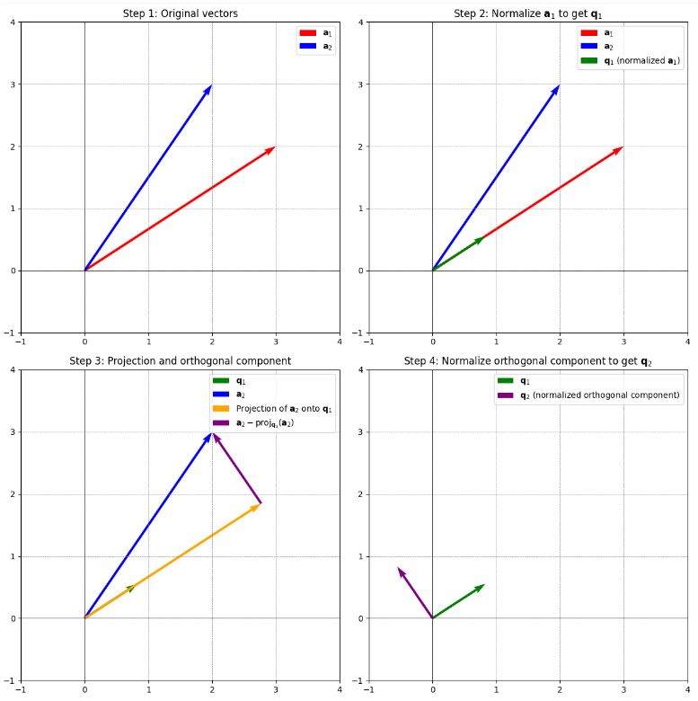
We then substract the components that overlap for each of those basis vectors, to get a \(q_i'\) that is linearly independent. We then normalise it and add it to the basis.
Current
Note has been deleted
Field-by-field Comparison
| Field | Before | After |
|---|---|---|
| Front | ||
| Back |
Note 1465: ETH::1. Semester::LinAlg
Deck: ETH::1. Semester::LinAlg
Note Type: Horvath Cloze
GUID:
deleted
Note Type: Horvath Cloze
GUID:
r,m&
Deleted Note
Front
Fundamental Subspaces:
Let \(A \in \mathbb{R}^{m \times n}\). \[ N(A) = C(A^\top)^\perp\]
Let \(A \in \mathbb{R}^{m \times n}\). \[ N(A) = C(A^\top)^\perp\]
Back
Fundamental Subspaces:
Let \(A \in \mathbb{R}^{m \times n}\). \[ N(A) = C(A^\top)^\perp\]
Let \(A \in \mathbb{R}^{m \times n}\). \[ N(A) = C(A^\top)^\perp\]
Current
Note has been deleted
Field-by-field Comparison
| Field | Before | After |
|---|---|---|
| Text |
Note 1466: ETH::1. Semester::LinAlg
Deck: ETH::1. Semester::LinAlg
Note Type: Horvath Cloze
GUID:
deleted
Note Type: Horvath Cloze
GUID:
rV0)C5{8PB
Deleted Note
Front
For \(A\) a matrix and \(M\) an invertible matrix:
\(\textbf{N}(A) = \){{c1::\(\textbf{N}(MA)\) (nullspace is the same)}}Back
For \(A\) a matrix and \(M\) an invertible matrix:
\(\textbf{N}(A) = \){{c1::\(\textbf{N}(MA)\) (nullspace is the same)}}Current
Note has been deleted
Field-by-field Comparison
| Field | Before | After |
|---|---|---|
| Text |
Note 1467: ETH::1. Semester::LinAlg
Deck: ETH::1. Semester::LinAlg
Note Type: Horvath Cloze
GUID:
deleted
Note Type: Horvath Cloze
GUID:
rX
Deleted Note
Front
Let \(V, W\) be two vector spaces. A function \(T: V \rightarrow W\) is called a linear transformation between vector spaces if the following linearity axiom holds for all \(x_1, x_2 \in V\) and all \(\lambda_1, \lambda_2 \in \mathbb{R}\): \[ T(\lambda_1 x_1 + \lambda_2 x_2) = \lambda_1 T(x_1) + \lambda_2 T(x_2) \]
Back
Let \(V, W\) be two vector spaces. A function \(T: V \rightarrow W\) is called a linear transformation between vector spaces if the following linearity axiom holds for all \(x_1, x_2 \in V\) and all \(\lambda_1, \lambda_2 \in \mathbb{R}\): \[ T(\lambda_1 x_1 + \lambda_2 x_2) = \lambda_1 T(x_1) + \lambda_2 T(x_2) \]
Current
Note has been deleted
Field-by-field Comparison
| Field | Before | After |
|---|---|---|
| Text |
Note 1468: ETH::1. Semester::LinAlg
Deck: ETH::1. Semester::LinAlg
Note Type: Horvath Cloze
GUID:
deleted
Note Type: Horvath Cloze
GUID:
re^L]
Deleted Note
Front
We can decompose \(\mathbb{R}^n = {{c1:: V + V^\bot = \{v + w \mid v \in V, w \in V^\bot\} }}\) using a Minkowsky sum.
Back
We can decompose \(\mathbb{R}^n = {{c1:: V + V^\bot = \{v + w \mid v \in V, w \in V^\bot\} }}\) using a Minkowsky sum.
We can also write \(\mathbb{R}^n = V^\bot + (V^\bot)^\bot\), it's symmetric.
Current
Note has been deleted
Field-by-field Comparison
| Field | Before | After |
|---|---|---|
| Text | ||
| Extra |
Note 1469: ETH::1. Semester::LinAlg
Deck: ETH::1. Semester::LinAlg
Note Type: Horvath Cloze
GUID:
deleted
Note Type: Horvath Cloze
GUID:
rj{~]5a9g*
Deleted Note
Front
Let \(A\) be an \(m \times n\) matrix and \(M\) an invertible \(m \times m\) matrix.
Then the two systems \(Ax = b\) and \(MAx = Mb\) have the same solutions \(x\).
Then the two systems \(Ax = b\) and \(MAx = Mb\) have the same solutions \(x\).
Back
Let \(A\) be an \(m \times n\) matrix and \(M\) an invertible \(m \times m\) matrix.
Then the two systems \(Ax = b\) and \(MAx = Mb\) have the same solutions \(x\).
Then the two systems \(Ax = b\) and \(MAx = Mb\) have the same solutions \(x\).
This is why Gauss-Jordan Elimination works.
Current
Note has been deleted
Field-by-field Comparison
| Field | Before | After |
|---|---|---|
| Text | ||
| Extra |
Note 1470: ETH::1. Semester::LinAlg
Deck: ETH::1. Semester::LinAlg
Note Type: Horvath Cloze
GUID:
deleted
Note Type: Horvath Cloze
GUID:
rn`#u|JmN0
Deleted Note
Front
For \(A\) a matrix and \(M\) an invertible matrix:
Back
For \(A\) a matrix and \(M\) an invertible matrix:
Current
Note has been deleted
Field-by-field Comparison
| Field | Before | After |
|---|---|---|
| Text |
Note 1471: ETH::1. Semester::LinAlg
Deck: ETH::1. Semester::LinAlg
Note Type: Horvath Cloze
GUID:
deleted
Note Type: Horvath Cloze
GUID:
rnuwKzI%R.
Deleted Note
Front
Let \(v_1, \dots, v_k\) be a basis of subspace \(V\). Let \(w_1, \dots, w_l\) be a basis of subspace \(W\).
\(V\) and \(W\) are orthogonal if and only if {{c1::\(v_i\) and \(w_j\) are orthogonal for all \(i \in \{1, \dots, k\}\) and \(j \in \{1, \dots, l\}\)}}.
\(V\) and \(W\) are orthogonal if and only if {{c1::\(v_i\) and \(w_j\) are orthogonal for all \(i \in \{1, \dots, k\}\) and \(j \in \{1, \dots, l\}\)}}.
Back
Let \(v_1, \dots, v_k\) be a basis of subspace \(V\). Let \(w_1, \dots, w_l\) be a basis of subspace \(W\).
\(V\) and \(W\) are orthogonal if and only if {{c1::\(v_i\) and \(w_j\) are orthogonal for all \(i \in \{1, \dots, k\}\) and \(j \in \{1, \dots, l\}\)}}.
\(V\) and \(W\) are orthogonal if and only if {{c1::\(v_i\) and \(w_j\) are orthogonal for all \(i \in \{1, \dots, k\}\) and \(j \in \{1, \dots, l\}\)}}.
Subspaces are orthogonal if their basis-vectors are orthogonal.
Current
Note has been deleted
Field-by-field Comparison
| Field | Before | After |
|---|---|---|
| Text | ||
| Extra |
Note 1472: ETH::1. Semester::LinAlg
Deck: ETH::1. Semester::LinAlg
Note Type: Horvath Cloze
GUID:
deleted
Note Type: Horvath Cloze
GUID:
rs*|Dcb_E|
Deleted Note
Front
For \(A\) written in CR-Decomposition \(A = CR'\), \(R'\) is unique.
Back
For \(A\) written in CR-Decomposition \(A = CR'\), \(R'\) is unique.
\(R'\) is unique because the \(C\) is linearly independent and there's only one way to write a vector (the columns of \(A\)) as the linear combination of independent vectors.
Current
Note has been deleted
Field-by-field Comparison
| Field | Before | After |
|---|---|---|
| Text | ||
| Extra |
Note 1473: ETH::1. Semester::LinAlg
Deck: ETH::1. Semester::LinAlg
Note Type: Horvath Cloze
GUID:
deleted
Note Type: Horvath Cloze
GUID:
rvqzRY-*GX
Deleted Note
Front
A diagonal matrix \(D\) has eigenvalues which are the diagonals and a full set of eigenvectors \(e_1, \dots, e_n\).
Back
A diagonal matrix \(D\) has eigenvalues which are the diagonals and a full set of eigenvectors \(e_1, \dots, e_n\).
Current
Note has been deleted
Field-by-field Comparison
| Field | Before | After |
|---|---|---|
| Text |
Note 1474: ETH::1. Semester::LinAlg
Deck: ETH::1. Semester::LinAlg
Note Type: Horvath Cloze
GUID:
deleted
Note Type: Horvath Cloze
GUID:
s!I_p%w(=W
Deleted Note
Front
Any degree \(n\) polynomial \(P(z)\) (with \(n \geq 1\)) has {{c1::\(n\) zeros \(\lambda_1, \dots, \lambda_n \in \mathbb{C}\)}}, possibly with repetitions, such that \[P(z) = a_n (z-\lambda_1)(z - \lambda_2) \cdots (z - \lambda_n)\]
Back
Any degree \(n\) polynomial \(P(z)\) (with \(n \geq 1\)) has {{c1::\(n\) zeros \(\lambda_1, \dots, \lambda_n \in \mathbb{C}\)}}, possibly with repetitions, such that \[P(z) = a_n (z-\lambda_1)(z - \lambda_2) \cdots (z - \lambda_n)\]
Current
Note has been deleted
Field-by-field Comparison
| Field | Before | After |
|---|---|---|
| Text |
Note 1475: ETH::1. Semester::LinAlg
Deck: ETH::1. Semester::LinAlg
Note Type: Horvath Cloze
GUID:
deleted
Note Type: Horvath Cloze
GUID:
s(K/=VnA_Y
Deleted Note
Front
We can write \(A\) as the sum of rank \(1\) matrices: \[A = {{c2::\sum_{k = 1}^n \lambda_i v_i v_i^\top}}\]where \(v_1, \dots, v_n\) are an orthonormal basis of eigenvectors (the \(V\) in diagonalisation) and \(\lambda_1, \dots, \lambda_n\) the associated eigenvectors.
Back
We can write \(A\) as the sum of rank \(1\) matrices: \[A = {{c2::\sum_{k = 1}^n \lambda_i v_i v_i^\top}}\]where \(v_1, \dots, v_n\) are an orthonormal basis of eigenvectors (the \(V\) in diagonalisation) and \(\lambda_1, \dots, \lambda_n\) the associated eigenvectors.
Current
Note has been deleted
Field-by-field Comparison
| Field | Before | After |
|---|---|---|
| Text |
Note 1476: ETH::1. Semester::LinAlg
Deck: ETH::1. Semester::LinAlg
Note Type: Horvath Cloze
GUID:
deleted
Note Type: Horvath Cloze
GUID:
s,(|c|R^[@
Deleted Note
Front
- If \(m = n\) (\(A\) is square), the system \(Ax = b\) is called square. Typically solvable.
- If \(m < n\) (A is a wide matrix), the system \(Ax = b\) is called underdetermined. These are typically solvable.
- If \(m > n\) (A is a tall matrix) the system \(Ax = b\) is called overdetermined. Typically not solvable.
Back
- If \(m = n\) (\(A\) is square), the system \(Ax = b\) is called square. Typically solvable.
- If \(m < n\) (A is a wide matrix), the system \(Ax = b\) is called underdetermined. These are typically solvable.
- If \(m > n\) (A is a tall matrix) the system \(Ax = b\) is called overdetermined. Typically not solvable.
(Undetermined because there are more variables than equations.)
Current
Note has been deleted
Field-by-field Comparison
| Field | Before | After |
|---|---|---|
| Text | ||
| Extra |
Note 1477: ETH::1. Semester::LinAlg
Deck: ETH::1. Semester::LinAlg
Note Type: Horvath Cloze
GUID:
deleted
Note Type: Horvath Cloze
GUID:
s-`w^:1S}3
Deleted Note
Front
Given \(n\) vectors \(v_1, \dots, v_n \in \mathbb{R}^n\) we call their Gram matrix the {{c2::\(n \times n\) matrix of inner products \(G_{ij} = v_i^\top v_j\)}}.
Back
Given \(n\) vectors \(v_1, \dots, v_n \in \mathbb{R}^n\) we call their Gram matrix the {{c2::\(n \times n\) matrix of inner products \(G_{ij} = v_i^\top v_j\)}}.
Current
Note has been deleted
Field-by-field Comparison
| Field | Before | After |
|---|---|---|
| Text |
Note 1478: ETH::1. Semester::LinAlg
Deck: ETH::1. Semester::LinAlg
Note Type: Horvath Classic
GUID:
deleted
Note Type: Horvath Classic
GUID:
s1Oa?:={wu
Deleted Note
Front
Does \(Av = v\) mean \(1\) is an eigenvalue of \(A\)?
Back
Does \(Av = v\) mean \(1\) is an eigenvalue of \(A\)?
No, we need to have \(v \neq 0\) to have that relationship hold!
Current
Note has been deleted
Field-by-field Comparison
| Field | Before | After |
|---|---|---|
| Front | ||
| Back |
Note 1479: ETH::1. Semester::LinAlg
Deck: ETH::1. Semester::LinAlg
Note Type: Horvath Classic
GUID:
deleted
Note Type: Horvath Classic
GUID:
s@:duB;6%y
Deleted Note
Front
What special conditions (other than the 3 basic conditions) make a set of vectors linearly dependent?
Back
What special conditions (other than the 3 basic conditions) make a set of vectors linearly dependent?
If:
- one of the vectors is 0
- one vector \(\textbf{v}\) is contained twice
Current
Note has been deleted
Field-by-field Comparison
| Field | Before | After |
|---|---|---|
| Front | ||
| Back |
Note 1480: ETH::1. Semester::LinAlg
Deck: ETH::1. Semester::LinAlg
Note Type: Horvath Cloze
GUID:
deleted
Note Type: Horvath Cloze
GUID:
sH/[5Mikuh
Deleted Note
Front
If \(A\) is a matrix and \(P\) is a permutation that swaps two elements (i.e. \(\text{sgn}(P) = -1\)): \[\det(PA) = - \det(A) \]
Back
If \(A\) is a matrix and \(P\) is a permutation that swaps two elements (i.e. \(\text{sgn}(P) = -1\)): \[\det(PA) = - \det(A) \]
\(PA\) corresponds to swapping two rows of \(A\)
Current
Note has been deleted
Field-by-field Comparison
| Field | Before | After |
|---|---|---|
| Text | ||
| Extra |
Note 1481: ETH::1. Semester::LinAlg
Deck: ETH::1. Semester::LinAlg
Note Type: Horvath Cloze
GUID:
deleted
Note Type: Horvath Cloze
GUID:
sQOMX5~Sf=
Deleted Note
Front
Matrix multiplication is not commutative most of the time.
Back
Matrix multiplication is not commutative most of the time.
Current
Note has been deleted
Field-by-field Comparison
| Field | Before | After |
|---|---|---|
| Text |
Note 1482: ETH::1. Semester::LinAlg
Deck: ETH::1. Semester::LinAlg
Note Type: Horvath Classic
GUID:
deleted
Note Type: Horvath Classic
GUID:
s`o%{8yLJx
Deleted Note
Front
How do we find a basis for the nullspace of \(A\)?
Back
How do we find a basis for the nullspace of \(A\)?
- Compute the RREF form \(R\) of \(A\) (\(MA\) has the same nullspace as \(A\): \(\textbf{N}(A) = \textbf{N}(MA)\))
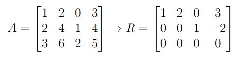
- Remove any zero rows (because \(0^\top x = 0\) regardless of \(x\))
- Solve for \(Rx = 0\):
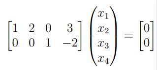
- We seperate the matrix into the identity and the "rest". Note that for this we take columns 1 and 2 as they form the 2x2 identity.
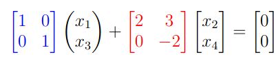
- Which becomes
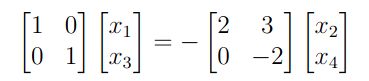
- We reduce this to a system of equations:
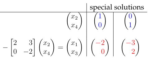 We choose two special solutions (independent) and then plug in the values into our equations to find the rest. This gives us a basis of the nullspace as we get two linearly independent vectors in there and it has dimension 2. We call these particular solutions.
Final nullspace:
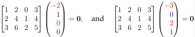
Current
Note has been deleted
Field-by-field Comparison
| Field | Before | After |
|---|---|---|
| Front | ||
| Back |
Note 1483: ETH::1. Semester::LinAlg
Deck: ETH::1. Semester::LinAlg
Note Type: Horvath Cloze
GUID:
deleted
Note Type: Horvath Cloze
GUID:
smJ/avn#*y
Deleted Note
Front
\(A^\top A\) is invertible if and only if \(A\) has linearly independent columns.
Back
\(A^\top A\) is invertible if and only if \(A\) has linearly independent columns.
Current
Note has been deleted
Field-by-field Comparison
| Field | Before | After |
|---|---|---|
| Text |
Note 1484: ETH::1. Semester::LinAlg
Deck: ETH::1. Semester::LinAlg
Note Type: Horvath Classic
GUID:
deleted
Note Type: Horvath Classic
GUID:
sp}Iuo:,06
Deleted Note
Front
How do we express the unit vectors of \(\mathbb{R}^n\)?
Back
How do we express the unit vectors of \(\mathbb{R}^n\)?
\(\{e_1, e_2, ... e_n\}\)
Current
Note has been deleted
Field-by-field Comparison
| Field | Before | After |
|---|---|---|
| Front | ||
| Back |
Note 1485: ETH::1. Semester::LinAlg
Deck: ETH::1. Semester::LinAlg
Note Type: Horvath Cloze
GUID:
deleted
Note Type: Horvath Cloze
GUID:
s},fJ+;VIc
Deleted Note
Front
\(A\) has an EW \(0\) \(\Longleftrightarrow\)\(A\) is not invertible Proof Included
Back
\(A\) has an EW \(0\) \(\Longleftrightarrow\)\(A\) is not invertible Proof Included
We know the EVs are in the \(N(A - \lambda I)\) because they solve the formula \(Av = \lambda v \implies Av - \lambda v \)\(= 0 \implies (A - \lambda I)v = 0\). Thus \(v\) is in the nullspace of \((A - \lambda I)\).
If \(A\) is not invertible, then it will have an EV of \(0\), which means that there is an EV solving \((A - 0 \cdot I)v = 0 \implies Av = 0\). Thus \(v \neq 0\) is in the nullspace of \(A\), i.e. the nullspace is not empty.
Current
Note has been deleted
Field-by-field Comparison
| Field | Before | After |
|---|---|---|
| Text | ||
| Extra |
Note 1486: ETH::1. Semester::LinAlg
Deck: ETH::1. Semester::LinAlg
Note Type: Horvath Cloze
GUID:
deleted
Note Type: Horvath Cloze
GUID:
t2:)I`&X*~
Deleted Note
Front
The projection of a vector \(b \in \mathbb{R}^m\) onto a subspace \(S\) (of \(\mathbb{R}^m\)) is the point in \(S\) that is closest to \(b\). In other words \[ \text{proj}_S(b) = {{c1:: \text{argmin}_{p \in S} ||b - p|| }}\]
Back
The projection of a vector \(b \in \mathbb{R}^m\) onto a subspace \(S\) (of \(\mathbb{R}^m\)) is the point in \(S\) that is closest to \(b\). In other words \[ \text{proj}_S(b) = {{c1:: \text{argmin}_{p \in S} ||b - p|| }}\]
Where \(b = p + e \implies b - p = e\), with \(e\) the error.
Current
Note has been deleted
Field-by-field Comparison
| Field | Before | After |
|---|---|---|
| Text | ||
| Extra |
Note 1487: ETH::1. Semester::LinAlg
Deck: ETH::1. Semester::LinAlg
Note Type: Horvath Cloze
GUID:
deleted
Note Type: Horvath Cloze
GUID:
t8F!:>0%NQ
Deleted Note
Front
The \(QR\) decomposition of an \(A\) with linearly independent columns is \(A = QR\) with \(Q\) orthogonal and \(R\) upper triangular.
Back
The \(QR\) decomposition of an \(A\) with linearly independent columns is \(A = QR\) with \(Q\) orthogonal and \(R\) upper triangular.
Current
Note has been deleted
Field-by-field Comparison
| Field | Before | After |
|---|---|---|
| Text |
Note 1488: ETH::1. Semester::LinAlg
Deck: ETH::1. Semester::LinAlg
Note Type: Horvath Cloze
GUID:
deleted
Note Type: Horvath Cloze
GUID:
tQtZJZ|Ls+
Deleted Note
Front
Given a real matrix \(A \in \mathbb{R}^{n \times n}\), the non-zero eigenvalues of \(A^\top A\) are the same ones as of \(AA^\top\).
Both matrices are symmetric and PSD.
Proof Included
Back
Given a real matrix \(A \in \mathbb{R}^{n \times n}\), the non-zero eigenvalues of \(A^\top A\) are the same ones as of \(AA^\top\).
Both matrices are symmetric and PSD.
Proof Included
Proof \(G = AA^\top\) and \(G = A^\top A\) are PSD.
- \(x^\top G x = x^\top (A^\top A ) x = (Ax)^\top (Ax) = ||Ax||^2 \geq 0\)
- \(x^\top G x = x^\top AA^\top x = (A^\top x)^\top (A^\top x) = ||A^\top x||^2 \geq 0\)
Current
Note has been deleted
Field-by-field Comparison
| Field | Before | After |
|---|---|---|
| Text | ||
| Extra |
Note 1489: ETH::1. Semester::LinAlg
Deck: ETH::1. Semester::LinAlg
Note Type: Horvath Cloze
GUID:
deleted
Note Type: Horvath Cloze
GUID:
tR&oOKzisO
Deleted Note
Front
A matrix decomposition is a factorization of a single matrix into a product of ones with useful properties.
Back
A matrix decomposition is a factorization of a single matrix into a product of ones with useful properties.
Example: LU decomposition (\(A=LU\))
Current
Note has been deleted
Field-by-field Comparison
| Field | Before | After |
|---|---|---|
| Text | ||
| Extra |
Note 1490: ETH::1. Semester::LinAlg
Deck: ETH::1. Semester::LinAlg
Note Type: Horvath Cloze
GUID:
deleted
Note Type: Horvath Cloze
GUID:
tX5`w6cN=$
Deleted Note
Front
Let \(a \in \mathbb{R}^m \ \backslash \ \{0\}\).
The projection of \(b \in \mathbb{R}^m\) on \(S = \{\lambda a \ | \ \lambda \in \mathbb{R} \} = C(a)\) is given by: \[ \text{proj}_S(b) = {{c1:: \frac{aa^\top}{a^\top a}b }}\]
This minimiser is unique.
Back
Let \(a \in \mathbb{R}^m \ \backslash \ \{0\}\).
The projection of \(b \in \mathbb{R}^m\) on \(S = \{\lambda a \ | \ \lambda \in \mathbb{R} \} = C(a)\) is given by: \[ \text{proj}_S(b) = {{c1:: \frac{aa^\top}{a^\top a}b }}\]
This minimiser is unique.
Current
Note has been deleted
Field-by-field Comparison
| Field | Before | After |
|---|---|---|
| Text |
Note 1491: ETH::1. Semester::LinAlg
Deck: ETH::1. Semester::LinAlg
Note Type: Horvath Cloze
GUID:
deleted
Note Type: Horvath Cloze
GUID:
tjub=34aze
Deleted Note
Front
\(AA^\dagger\) is symmetric.
Back
\(AA^\dagger\) is symmetric.
Current
Note has been deleted
Field-by-field Comparison
| Field | Before | After |
|---|---|---|
| Text |
Note 1492: ETH::1. Semester::LinAlg
Deck: ETH::1. Semester::LinAlg
Note Type: Horvath Cloze
GUID:
deleted
Note Type: Horvath Cloze
GUID:
tr&k>HpzdT
Deleted Note
Front
A basis is not always a set of vectors, it could also be a set of matrices.
Back
A basis is not always a set of vectors, it could also be a set of matrices.
Thus for the subspace of diagonal matrices \(D_m\), the basis is made up of diagonal matrices.
Current
Note has been deleted
Field-by-field Comparison
| Field | Before | After |
|---|---|---|
| Text | ||
| Extra |
Note 1493: ETH::1. Semester::LinAlg
Deck: ETH::1. Semester::LinAlg
Note Type: Horvath Classic
GUID:
deleted
Note Type: Horvath Classic
GUID:
u8Qxy,>bCQ
Deleted Note
Front
Let \(A \in \mathbb{R}^{m \times m}\). \(A\) is invertible if:
Back
Let \(A \in \mathbb{R}^{m \times m}\). \(A\) is invertible if:
There is a \(m \times m\) matrix \(B\) such that \(BA = I\).
Exists only if \(A\) has linearly independent columns.
Exists only if \(A\) has linearly independent columns.
Current
Note has been deleted
Field-by-field Comparison
| Field | Before | After |
|---|---|---|
| Front | ||
| Back |
Note 1494: ETH::1. Semester::LinAlg
Deck: ETH::1. Semester::LinAlg
Note Type: Horvath Cloze
GUID:
deleted
Note Type: Horvath Cloze
GUID:
u9EK]1)kgH
Deleted Note
Front
We have \(C(Q) =\) \(C(A)\) for \(Q\) the result of Gram-Schmidt on \(A\).
Back
We have \(C(Q) =\) \(C(A)\) for \(Q\) the result of Gram-Schmidt on \(A\).
Current
Note has been deleted
Field-by-field Comparison
| Field | Before | After |
|---|---|---|
| Text |
Note 1495: ETH::1. Semester::LinAlg
Deck: ETH::1. Semester::LinAlg
Note Type: Horvath Cloze
GUID:
deleted
Note Type: Horvath Cloze
GUID:
u:|nk(8Sda
Deleted Note
Front
The co-factors of \(A\) are \( C_{ij} = {{c1:: (-1)^{i + j} \det(\mathcal{A}_{ij}) }}\) where \(\mathcal{A}_{ij}\) is the \((n - 1)\times (n-1)\) matrix without row \(i\) and column \(j\).
Back
The co-factors of \(A\) are \( C_{ij} = {{c1:: (-1)^{i + j} \det(\mathcal{A}_{ij}) }}\) where \(\mathcal{A}_{ij}\) is the \((n - 1)\times (n-1)\) matrix without row \(i\) and column \(j\).

Current
Note has been deleted
Field-by-field Comparison
| Field | Before | After |
|---|---|---|
| Text | ||
| Extra |
Note 1496: ETH::1. Semester::LinAlg
Deck: ETH::1. Semester::LinAlg
Note Type: Horvath Cloze
GUID:
deleted
Note Type: Horvath Cloze
GUID:
uCC
Deleted Note
Front
The \(\text{sgn}(\sigma)\) where \(\sigma\) is a permutation is {{c1::the parity of the number of elements that are out of order (inversions: \( i < j \text{ and } \sigma(i) > \sigma( j)\)) after applying the permutation::inversions}}.
Back
The \(\text{sgn}(\sigma)\) where \(\sigma\) is a permutation is {{c1::the parity of the number of elements that are out of order (inversions: \( i < j \text{ and } \sigma(i) > \sigma( j)\)) after applying the permutation::inversions}}.
\((1, 3, 2)\) has one inversion.
\(\text{sgn}(\sigma)=(−1)^k\) where \(k\) is the number of transpositions (swaps) needed to obtain \(σ\) from the identity.
\(\text{sgn}(\sigma)=(−1)^k\) where \(k\) is the number of transpositions (swaps) needed to obtain \(σ\) from the identity.
Current
Note has been deleted
Field-by-field Comparison
| Field | Before | After |
|---|---|---|
| Text | ||
| Extra |
Note 1497: ETH::1. Semester::LinAlg
Deck: ETH::1. Semester::LinAlg
Note Type: Horvath Classic
GUID:
deleted
Note Type: Horvath Classic
GUID:
uWwT2a*Vb[
Deleted Note
Front
What is the nullspace of a matrix?
Back
What is the nullspace of a matrix?
The set of vectors that give the 0-vector when multiplied with the given matrix.
\(N(A) := \{x\in \mathbb{R} : Ax = \boldsymbol{0} \}\)
\(N(A) := \{x\in \mathbb{R} : Ax = \boldsymbol{0} \}\)
Current
Note has been deleted
Field-by-field Comparison
| Field | Before | After |
|---|---|---|
| Front | ||
| Back |
Note 1498: ETH::1. Semester::LinAlg
Deck: ETH::1. Semester::LinAlg
Note Type: Horvath Cloze
GUID:
deleted
Note Type: Horvath Cloze
GUID:
u^,*N^?pR/
Deleted Note
Front
A symmetric matrix \(A \in \mathbb{R}^{n \times n}\) is positive definite if and only if {{c2::\(x^\top Ax > 0\) for all \(x \in \mathbb{R}^n \setminus \{0\}\)}}.
Back
A symmetric matrix \(A \in \mathbb{R}^{n \times n}\) is positive definite if and only if {{c2::\(x^\top Ax > 0\) for all \(x \in \mathbb{R}^n \setminus \{0\}\)}}.
Current
Note has been deleted
Field-by-field Comparison
| Field | Before | After |
|---|---|---|
| Text |
Note 1499: ETH::1. Semester::LinAlg
Deck: ETH::1. Semester::LinAlg
Note Type: Horvath Cloze
GUID:
deleted
Note Type: Horvath Cloze
GUID:
uamL=`piJf
Deleted Note
Front
The sign of a permutation is multiplicative:
\(\text{sgn}(\sigma \circ \lambda) = {{c1:: \text{sgn}(\sigma) \cdot \text{sgn}(\lambda)}}\).
\(\text{sgn}(\sigma \circ \lambda) = {{c1:: \text{sgn}(\sigma) \cdot \text{sgn}(\lambda)}}\).
Back
The sign of a permutation is multiplicative:
\(\text{sgn}(\sigma \circ \lambda) = {{c1:: \text{sgn}(\sigma) \cdot \text{sgn}(\lambda)}}\).
\(\text{sgn}(\sigma \circ \lambda) = {{c1:: \text{sgn}(\sigma) \cdot \text{sgn}(\lambda)}}\).
Current
Note has been deleted
Field-by-field Comparison
| Field | Before | After |
|---|---|---|
| Text |
Note 1500: ETH::1. Semester::LinAlg
Deck: ETH::1. Semester::LinAlg
Note Type: Horvath Cloze
GUID:
deleted
Note Type: Horvath Cloze
GUID:
uo#Gn+y8bD
Deleted Note
Front
Für alle Vektorpaare \( \mathbf{x,y} \in \mathbb{E}^n \) gilt die Cauchy-Schwarz-Ungleichung: {{c1::\( | \langle \mathbf{x, y} \rangle | \le ||\mathbf{x}|| \ ||\mathbf{y}||\)}}
Back
Für alle Vektorpaare \( \mathbf{x,y} \in \mathbb{E}^n \) gilt die Cauchy-Schwarz-Ungleichung: {{c1::\( | \langle \mathbf{x, y} \rangle | \le ||\mathbf{x}|| \ ||\mathbf{y}||\)}}
Current
Note has been deleted
Field-by-field Comparison
| Field | Before | After |
|---|---|---|
| Text |
Note 1501: ETH::1. Semester::LinAlg
Deck: ETH::1. Semester::LinAlg
Note Type: Horvath Cloze
GUID:
deleted
Note Type: Horvath Cloze
GUID:
uodougE6kh
Deleted Note
Front
The determinant exists only for square matrices.
Back
The determinant exists only for square matrices.
Current
Note has been deleted
Field-by-field Comparison
| Field | Before | After |
|---|---|---|
| Text |
Note 1502: ETH::1. Semester::LinAlg
Deck: ETH::1. Semester::LinAlg
Note Type: Horvath Cloze
GUID:
deleted
Note Type: Horvath Cloze
GUID:
uqAA$|?Lip
Deleted Note
Front
Let \(A \in \mathbb{R}^{n \times n}\) be a symmetric matrix and \(\lambda_1 \neq \lambda_2 \in \mathbb{R}\) two distinct eigenvalues of \(A\) with corresponding eigenvectors \(v_1, v_2\).
Then \(v_1\) and \(v_2\) are orthogonal. Proof Included
Back
Let \(A \in \mathbb{R}^{n \times n}\) be a symmetric matrix and \(\lambda_1 \neq \lambda_2 \in \mathbb{R}\) two distinct eigenvalues of \(A\) with corresponding eigenvectors \(v_1, v_2\).
Then \(v_1\) and \(v_2\) are orthogonal. Proof Included
\(\lambda_1 v_1 ^\top v_2 = (Av_1)^\top v_2\) \( = v_1^\top A ^\top v_2 = \) \(v_1^\top (Av_2)\) \( = \lambda_2 v_1^\top v_2\)
Current
Note has been deleted
Field-by-field Comparison
| Field | Before | After |
|---|---|---|
| Text | ||
| Extra |
Note 1503: ETH::1. Semester::LinAlg
Deck: ETH::1. Semester::LinAlg
Note Type: Horvath Cloze
GUID:
deleted
Note Type: Horvath Cloze
GUID:
v#FTBh.m{S
Deleted Note
Front
Ein LGS heisst homogen, wenn die rechte Seite Null ist.
Back
Ein LGS heisst homogen, wenn die rechte Seite Null ist.
Besitzt immer triviale Lösung (alles 0).
Current
Note has been deleted
Field-by-field Comparison
| Field | Before | After |
|---|---|---|
| Text | ||
| Extra |
Note 1504: ETH::1. Semester::LinAlg
Deck: ETH::1. Semester::LinAlg
Note Type: Horvath Cloze
GUID:
deleted
Note Type: Horvath Cloze
GUID:
v>PZpE,mn~
Deleted Note
Front
Let \(V\) be a finitely generated vector space, \(F \subseteq V\) a finite set of linearly independent vectors (note that \(F\) does not need to span \(V\)) and \(G \subseteq V\) a finite set of vectors with \(\textbf{Span}(G) = V\) (but they don't all need to be independent). Then the following two statements hold:
- \(|F| \leq |G|\)
- {{c2::There exists a subset \(E \subseteq G\) of size \(|G| - |F|\) such that \(\textbf{Span}(F \cup E) = V\).}}
Back
Let \(V\) be a finitely generated vector space, \(F \subseteq V\) a finite set of linearly independent vectors (note that \(F\) does not need to span \(V\)) and \(G \subseteq V\) a finite set of vectors with \(\textbf{Span}(G) = V\) (but they don't all need to be independent). Then the following two statements hold:
- \(|F| \leq |G|\)
- {{c2::There exists a subset \(E \subseteq G\) of size \(|G| - |F|\) such that \(\textbf{Span}(F \cup E) = V\).}}
We can use the lemma to argue that there can't be more than \(n\) independent vectors in a space of dimension \(n\).
Current
Note has been deleted
Field-by-field Comparison
| Field | Before | After |
|---|---|---|
| Text | ||
| Extra |
Note 1505: ETH::1. Semester::LinAlg
Deck: ETH::1. Semester::LinAlg
Note Type: Horvath Classic
GUID:
deleted
Note Type: Horvath Classic
GUID:
vA(v{*KZt+
Deleted Note
Front
In QR decomposition \(R\) is invertible because?
Back
In QR decomposition \(R\) is invertible because?
\(N(A) = \{0\}\) since \(A\) has independent columns and thus \(N(R) = \{0\}\):
- \(Rx = 0\) then \(Ax = QRx = 0\) thus \(Q\cdot 0 = 0\)
- Thus \(x \in N(A) \implies x = 0\)
Current
Note has been deleted
Field-by-field Comparison
| Field | Before | After |
|---|---|---|
| Front | ||
| Back |
Note 1506: ETH::1. Semester::LinAlg
Deck: ETH::1. Semester::LinAlg
Note Type: Horvath Classic
GUID:
deleted
Note Type: Horvath Classic
GUID:
vFzsuS+[?6
Deleted Note
Front
What is the columnspace of a matrix?
Back
What is the columnspace of a matrix?
The span of all column-vectors.
Current
Note has been deleted
Field-by-field Comparison
| Field | Before | After |
|---|---|---|
| Front | ||
| Back |
Note 1507: ETH::1. Semester::LinAlg
Deck: ETH::1. Semester::LinAlg
Note Type: Horvath Classic
GUID:
deleted
Note Type: Horvath Classic
GUID:
vMw:@b$pAy
Deleted Note
Front
How to recover a matrix \(A\) from it's eigenvectors and eigenvalues (complete set)?
Back
How to recover a matrix \(A\) from it's eigenvectors and eigenvalues (complete set)?
\(V\) the matrix with the eigenvectors of \(A\), orthogonal. Then we know \(AV = VD\) (\(Av_i = \lambda_i v_i\) in matrix form), with \(D = \Lambda\) the matrix with the eigenvalues on the diagonal.
Thus \(AVV^\top = VDV^\top \implies A = VDV^\top\) .
Thus \(AVV^\top = VDV^\top \implies A = VDV^\top\) .
Current
Note has been deleted
Field-by-field Comparison
| Field | Before | After |
|---|---|---|
| Front | ||
| Back |
Note 1508: ETH::1. Semester::LinAlg
Deck: ETH::1. Semester::LinAlg
Note Type: Horvath Classic
GUID:
deleted
Note Type: Horvath Classic
GUID:
v`BTz<1Q{~
Deleted Note
Front
Wann ist eine Matrix invertierbar?
Back
Wann ist eine Matrix invertierbar?
Falls eine Matrix \( \mathbf{X} \) existiert, sodass \( \mathbf{AX} = \mathbf{XA} = \mathbf{I_n}\)
Beispiel: \( \begin{pmatrix} 1 & 2 \\ 0 & 3 \end{pmatrix} * \begin{pmatrix} 1 & -\frac{2}{3} \\ 0 & \frac{1}{3} \end{pmatrix} = \mathbf{I_2}\)
Current
Note has been deleted
Field-by-field Comparison
| Field | Before | After |
|---|---|---|
| Front | ||
| Back |
Note 1509: ETH::1. Semester::LinAlg
Deck: ETH::1. Semester::LinAlg
Note Type: Horvath Cloze
GUID:
deleted
Note Type: Horvath Cloze
GUID:
ve7Q_/^p1y
Deleted Note
Front
For \(A \in \mathbb{R}^{m \times n}\) with \(\text{rank}(A) = m\), we define the pseudo-inverse \(A^\dagger \in \mathbb{R}^{n \times m}\) as:\[ A^\dagger = {{c1::A^\top (A A^\top)^{-1} }}\]
Back
For \(A \in \mathbb{R}^{m \times n}\) with \(\text{rank}(A) = m\), we define the pseudo-inverse \(A^\dagger \in \mathbb{R}^{n \times m}\) as:\[ A^\dagger = {{c1::A^\top (A A^\top)^{-1} }}\]
For an \(A\) with full column-rank, we basically define, \(A^\dagger\) as the transpose of the pseudoinverse of the transpose:
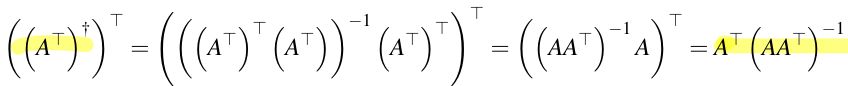
Current
Note has been deleted
Field-by-field Comparison
| Field | Before | After |
|---|---|---|
| Text | ||
| Extra |
Note 1510: ETH::1. Semester::LinAlg
Deck: ETH::1. Semester::LinAlg
Note Type: Horvath Cloze
GUID:
deleted
Note Type: Horvath Cloze
GUID:
ve95W6~[iY
Deleted Note
Front
For a projection to exist using our formula \(P = A (A^\top A)^{-1} A^\top\) we need \(A\) to have independent columns, i.e. they form a basis for \(C(A)\).
Back
For a projection to exist using our formula \(P = A (A^\top A)^{-1} A^\top\) we need \(A\) to have independent columns, i.e. they form a basis for \(C(A)\).
Otherwise the projection is not unique.
Current
Note has been deleted
Field-by-field Comparison
| Field | Before | After |
|---|---|---|
| Text | ||
| Extra |
Note 1511: ETH::1. Semester::LinAlg
Deck: ETH::1. Semester::LinAlg
Note Type: Horvath Classic
GUID:
deleted
Note Type: Horvath Classic
GUID:
vlkuMD-Ica
Deleted Note
Front
Was ist eine konjugiert-komplexe Matrix?
Back
Was ist eine konjugiert-komplexe Matrix?
Wenn \(\mathbf{A}\) eine komplexe Matrix ist, dann ist \(\overline{\mathbf{A}}\) mit \( (\overline{\mathbf{A}})_{ij} = \overline{(\mathbf{A})_{ij}}\) die konjugiert-komplexe Matrix.
Current
Note has been deleted
Field-by-field Comparison
| Field | Before | After |
|---|---|---|
| Front | ||
| Back |
Note 1512: ETH::1. Semester::LinAlg
Deck: ETH::1. Semester::LinAlg
Note Type: Horvath Classic
GUID:
deleted
Note Type: Horvath Classic
GUID:
vo=
Deleted Note
Front
What is a property of symmetrical matrices?
Back
What is a property of symmetrical matrices?
\(A^T = A\)
Current
Note has been deleted
Field-by-field Comparison
| Field | Before | After |
|---|---|---|
| Front | ||
| Back |
Note 1513: ETH::1. Semester::LinAlg
Deck: ETH::1. Semester::LinAlg
Note Type: Horvath Classic
GUID:
deleted
Note Type: Horvath Classic
GUID:
vp8-Q1S6eI
Deleted Note
Front
What holds for \(T(X+Y)?\)
Back
What holds for \(T(X+Y)?\)
\(= T(X) + T(Y)\)
Current
Note has been deleted
Field-by-field Comparison
| Field | Before | After |
|---|---|---|
| Front | ||
| Back |
Note 1514: ETH::1. Semester::LinAlg
Deck: ETH::1. Semester::LinAlg
Note Type: Horvath Cloze
GUID:
deleted
Note Type: Horvath Cloze
GUID:
v~twgkx^)U
Deleted Note
Front
For \(A \in \mathbb{R}^{m \times n}\) with \(\text{rank}(A) = r\) and CR decomposition \(A = CR\), we define the pseudoinverse \(A^\dagger\) as: \[ A^\dagger = R^\dagger C^\dagger \]
Back
For \(A \in \mathbb{R}^{m \times n}\) with \(\text{rank}(A) = r\) and CR decomposition \(A = CR\), we define the pseudoinverse \(A^\dagger\) as: \[ A^\dagger = R^\dagger C^\dagger \]
We can rewrite this as:
\(\begin{aligned} A^\dagger &= R^\top (RR^\top)^{-1} (C^\top C)^{-1} C^\top \\ &= R^\top (C^\top C R R^\top)^{-1} C^\top \\ &= R^\top (C^\top A R^\top)^{-1} C^\top \end{aligned}\)
\(\begin{aligned} A^\dagger &= R^\top (RR^\top)^{-1} (C^\top C)^{-1} C^\top \\ &= R^\top (C^\top C R R^\top)^{-1} C^\top \\ &= R^\top (C^\top A R^\top)^{-1} C^\top \end{aligned}\)
Current
Note has been deleted
Field-by-field Comparison
| Field | Before | After |
|---|---|---|
| Text | ||
| Extra |
Note 1515: ETH::1. Semester::LinAlg
Deck: ETH::1. Semester::LinAlg
Note Type: Horvath Cloze
GUID:
deleted
Note Type: Horvath Cloze
GUID:
w49b;wY}uY
Deleted Note
Front
The {{c2::rank of a matrix \(\textbf{rank}(A), A \in \mathbb{R}^{m \times n}\) is a number between 0 and n}} which counts the number of independent columns.
Back
The {{c2::rank of a matrix \(\textbf{rank}(A), A \in \mathbb{R}^{m \times n}\) is a number between 0 and n}} which counts the number of independent columns.
A column is independent if it is not the linear combination of the previous ones (or the next ones, if you do it the other way round).
Current
Note has been deleted
Field-by-field Comparison
| Field | Before | After |
|---|---|---|
| Text | ||
| Extra |
Note 1516: ETH::1. Semester::LinAlg
Deck: ETH::1. Semester::LinAlg
Note Type: Horvath Cloze
GUID:
deleted
Note Type: Horvath Cloze
GUID:
w6-9Dxu?
Deleted Note
Front
We call the solution space of \(Ax = b\) an affine subspace if \(b \neq 0\).
Back
We call the solution space of \(Ax = b\) an affine subspace if \(b \neq 0\).
Current
Note has been deleted
Field-by-field Comparison
| Field | Before | After |
|---|---|---|
| Text |
Note 1517: ETH::1. Semester::LinAlg
Deck: ETH::1. Semester::LinAlg
Note Type: Horvath Cloze
GUID:
deleted
Note Type: Horvath Cloze
GUID:
w7_|F6Nt!U
Deleted Note
Front
The triangle inequality \(||v|| + ||w|| \geq ||v+w||\) holds exactly if \(w = \lambda v\) for some \(\lambda\geq0\) (i.e., they point in the same direction).
Back
The triangle inequality \(||v|| + ||w|| \geq ||v+w||\) holds exactly if \(w = \lambda v\) for some \(\lambda\geq0\) (i.e., they point in the same direction).
Current
Note has been deleted
Field-by-field Comparison
| Field | Before | After |
|---|---|---|
| Text |
Note 1518: ETH::1. Semester::LinAlg
Deck: ETH::1. Semester::LinAlg
Note Type: Horvath Cloze
GUID:
deleted
Note Type: Horvath Cloze
GUID:
w9]Tx{V20J
Deleted Note
Front
For a complex vector \(v\) we have \(||v|| =\) {{c1:: \(v^*v = \overline{v}^\top v = \sum_{i = 1}^n \overline{v_i}v_i = \sum_{i = 1}^n |v_i|^2\)}}.
Back
For a complex vector \(v\) we have \(||v|| =\) {{c1:: \(v^*v = \overline{v}^\top v = \sum_{i = 1}^n \overline{v_i}v_i = \sum_{i = 1}^n |v_i|^2\)}}.
Current
Note has been deleted
Field-by-field Comparison
| Field | Before | After |
|---|---|---|
| Text |
Note 1519: ETH::1. Semester::LinAlg
Deck: ETH::1. Semester::LinAlg
Note Type: Horvath Classic
GUID:
deleted
Note Type: Horvath Classic
GUID:
w;_;AaM4pf
Deleted Note
Front
Was ist eine symmetrische Matrix?
Back
Was ist eine symmetrische Matrix?
Eine symmetrische Matrix erfüllt \(A^\top = A\) (d.h. eine "Spiegelachse" an der Hauptdiagonale). Hauptdiagonale selber unwichtig!
Beispiel:
\( \begin{pmatrix} 0 & 5 & 1 \\ 5 & 2 & 4 \\ 1 & 4 & 0 \end{pmatrix} \)
Current
Note has been deleted
Field-by-field Comparison
| Field | Before | After |
|---|---|---|
| Front | ||
| Back |
Note 1520: ETH::1. Semester::LinAlg
Deck: ETH::1. Semester::LinAlg
Note Type: Horvath Cloze
GUID:
deleted
Note Type: Horvath Cloze
GUID:
wGNTPZMph;
Deleted Note
Front
The \(\text{sgn}(\sigma)\) where \(\sigma\) is a permutation is the parity of the number of row swaps necessary to get back to the identity .
Back
The \(\text{sgn}(\sigma)\) where \(\sigma\) is a permutation is the parity of the number of row swaps necessary to get back to the identity .
Current
Note has been deleted
Field-by-field Comparison
| Field | Before | After |
|---|---|---|
| Text |
Note 1521: ETH::1. Semester::LinAlg
Deck: ETH::1. Semester::LinAlg
Note Type: Horvath Classic
GUID:
deleted
Note Type: Horvath Classic
GUID:
wl,mf){>,^
Deleted Note
Front
What is the 1-norm of a vector?
Back
What is the 1-norm of a vector?
Given a vector \(\mathbf{v} = (v_1, v_2, ..., v_n)^\top\):
\(||\mathbf{v}||_1 = \sum_{i=1}^n |v_i|\)
\(||\mathbf{v}||_1 = \sum_{i=1}^n |v_i|\)
Current
Note has been deleted
Field-by-field Comparison
| Field | Before | After |
|---|---|---|
| Front | ||
| Back |
Note 1522: ETH::1. Semester::LinAlg
Deck: ETH::1. Semester::LinAlg
Note Type: Horvath Classic
GUID:
deleted
Note Type: Horvath Classic
GUID:
wn-OubLttB
Deleted Note
Front
Is a basis for a vector space unique?
Back
Is a basis for a vector space unique?
No, there are typically many bases for a vector space.
Every set \(B = \{v_1, v_2, \dots, v_m\} \subseteq \mathbb{R}^m\) of linearly independent vectors is a basis of \(\mathbb{R}^m\).
Every set \(B = \{v_1, v_2, \dots, v_m\} \subseteq \mathbb{R}^m\) of linearly independent vectors is a basis of \(\mathbb{R}^m\).
Current
Note has been deleted
Field-by-field Comparison
| Field | Before | After |
|---|---|---|
| Front | ||
| Back |
Note 1523: ETH::1. Semester::LinAlg
Deck: ETH::1. Semester::LinAlg
Note Type: Horvath Cloze
GUID:
deleted
Note Type: Horvath Cloze
GUID:
wsmlD&i>fV
Deleted Note
Front
Projection is idempotent: \(PPb = Pb\) i.e. \(P^2 = P\).
Back
Projection is idempotent: \(PPb = Pb\) i.e. \(P^2 = P\).
When we project a vector already in the subspace, we simply get the same vector out.
Current
Note has been deleted
Field-by-field Comparison
| Field | Before | After |
|---|---|---|
| Text | ||
| Extra |
Note 1524: ETH::1. Semester::LinAlg
Deck: ETH::1. Semester::LinAlg
Note Type: Horvath Cloze
GUID:
deleted
Note Type: Horvath Cloze
GUID:
ww{@M/WDmP
Deleted Note
Front
\(A\) and \(A^\top\) share eigenvalues not eigenvectors.
Back
\(A\) and \(A^\top\) share eigenvalues not eigenvectors.
Current
Note has been deleted
Field-by-field Comparison
| Field | Before | After |
|---|---|---|
| Text |
Note 1525: ETH::1. Semester::LinAlg
Deck: ETH::1. Semester::LinAlg
Note Type: Horvath Classic
GUID:
deleted
Note Type: Horvath Classic
GUID:
w{ro)4tDv:
Deleted Note
Front
Pseudoinverse of \(A = \begin{bmatrix} 3 & 0 & 0 \\ 0 & 2 & 0 \end{bmatrix}\)?
Hint: It's already in SVD-form.
Hint: It's already in SVD-form.
Back
Pseudoinverse of \(A = \begin{bmatrix} 3 & 0 & 0 \\ 0 & 2 & 0 \end{bmatrix}\)?
Hint: It's already in SVD-form.
Hint: It's already in SVD-form.
Already in “SVD form” with \(U = I_2\), \(V = I_3\), and \(\Sigma = \begin{pmatrix} 3 & 0 & 0 \\ 0 & 2 & 0 \end{pmatrix}\).
The pseudoinverse is: \[A^\dagger = \begin{pmatrix} \frac{1}{3} & 0 \\ 0 & \frac{1}{2} \\ 0 & 0 \end{pmatrix}\] Notice:
- Shape flipped: \(A\) is \(2\times3\), so \(A^\dagger\) is \(3\times2\)
- Nonzero values inverted: \(3 \to \frac{1}{3}\), \(2 \to \frac{1}{2}\)
- Zeros stay zero
Current
Note has been deleted
Field-by-field Comparison
| Field | Before | After |
|---|---|---|
| Front | ||
| Back |
Note 1526: ETH::1. Semester::LinAlg
Deck: ETH::1. Semester::LinAlg
Note Type: Horvath Classic
GUID:
deleted
Note Type: Horvath Classic
GUID:
x4{!d?wKd.
Deleted Note
Front
What is the span of a set of vectors?
Back
What is the span of a set of vectors?
The span is defined as the set of all linear combinations:
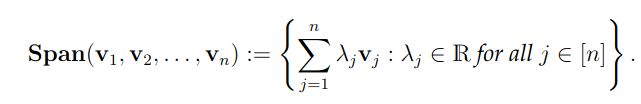
Current
Note has been deleted
Field-by-field Comparison
| Field | Before | After |
|---|---|---|
| Front | ||
| Back |
Note 1527: ETH::1. Semester::LinAlg
Deck: ETH::1. Semester::LinAlg
Note Type: Horvath Classic
GUID:
deleted
Note Type: Horvath Classic
GUID:
x5dCNKqS
Deleted Note
Front
Does a diagonalisable / diagonalised matrix have to be invertible?
Back
Does a diagonalisable / diagonalised matrix have to be invertible?
No it can have \(0\) eigenvalues.
Current
Note has been deleted
Field-by-field Comparison
| Field | Before | After |
|---|---|---|
| Front | ||
| Back |
Note 1528: ETH::1. Semester::LinAlg
Deck: ETH::1. Semester::LinAlg
Note Type: Horvath Cloze
GUID:
deleted
Note Type: Horvath Cloze
GUID:
xBE,c~;Xop
Deleted Note
Front
A \(1\times n\) matrix is called row vector or, in other contexts, tuple.
Back
A \(1\times n\) matrix is called row vector or, in other contexts, tuple.
Current
Note has been deleted
Field-by-field Comparison
| Field | Before | After |
|---|---|---|
| Text |
Note 1529: ETH::1. Semester::LinAlg
Deck: ETH::1. Semester::LinAlg
Note Type: Horvath Cloze
GUID:
deleted
Note Type: Horvath Cloze
GUID:
xFvw{LdP48
Deleted Note
Front
In the SVD:
- \(\Sigma \in \mathbb{R}^{m \times n}\) is {{c1::a diagonal matrix (in the sense that \(\Sigma_{ij} = 0\) when \(i \neq j\) and the diagonal values are non-negative and ordered in descending order)}}.
- \(U^\top U = I\) and \(V^\top V = I\) (\(U, V\) are orthogonal).
- The columns \(u_1, \dots, u_m\) of \(U\) are called the left-singular vectors of \(A\) and are orthonormal.
- The columns \(v_1, \dots, v_n\) of \(V\) are called the right-singular vectors of \(A\) and are orthonormal.
Back
In the SVD:
- \(\Sigma \in \mathbb{R}^{m \times n}\) is {{c1::a diagonal matrix (in the sense that \(\Sigma_{ij} = 0\) when \(i \neq j\) and the diagonal values are non-negative and ordered in descending order)}}.
- \(U^\top U = I\) and \(V^\top V = I\) (\(U, V\) are orthogonal).
- The columns \(u_1, \dots, u_m\) of \(U\) are called the left-singular vectors of \(A\) and are orthonormal.
- The columns \(v_1, \dots, v_n\) of \(V\) are called the right-singular vectors of \(A\) and are orthonormal.
Current
Note has been deleted
Field-by-field Comparison
| Field | Before | After |
|---|---|---|
| Text |
Note 1530: ETH::1. Semester::LinAlg
Deck: ETH::1. Semester::LinAlg
Note Type: Horvath Cloze
GUID:
deleted
Note Type: Horvath Cloze
GUID:
xK>u_ueFdY
Deleted Note
Front
Gaussian Elimination does not preserve EWs or EVs.
Back
Gaussian Elimination does not preserve EWs or EVs.
This means the EVs and EWs depend on the representation of the matrix, not on the subspaces they define.
Current
Note has been deleted
Field-by-field Comparison
| Field | Before | After |
|---|---|---|
| Text | ||
| Extra |
Note 1531: ETH::1. Semester::LinAlg
Deck: ETH::1. Semester::LinAlg
Note Type: Horvath Cloze
GUID:
deleted
Note Type: Horvath Cloze
GUID:
xn@gm`7I_o
Deleted Note
Front
Eine Linearkombination (LK) der Vektoren \( a_1, \ldots, a_n\) ist {{c2::ein Ausdruck der Form \( \alpha_1 a_1 + \cdots + \alpha_n a_n\) wobei \( \alpha_1, \ldots, \alpha_n \in \mathbb{R}\)}}
Back
Eine Linearkombination (LK) der Vektoren \( a_1, \ldots, a_n\) ist {{c2::ein Ausdruck der Form \( \alpha_1 a_1 + \cdots + \alpha_n a_n\) wobei \( \alpha_1, \ldots, \alpha_n \in \mathbb{R}\)}}
Current
Note has been deleted
Field-by-field Comparison
| Field | Before | After |
|---|---|---|
| Text |
Note 1532: ETH::1. Semester::LinAlg
Deck: ETH::1. Semester::LinAlg
Note Type: Horvath Cloze
GUID:
deleted
Note Type: Horvath Cloze
GUID:
xs#S^-Mehy
Deleted Note
Front
\(\det (A^{-1}) =\) {{c1::\((\det (A))^{-1}\)}}
Back
\(\det (A^{-1}) =\) {{c1::\((\det (A))^{-1}\)}}
Current
Note has been deleted
Field-by-field Comparison
| Field | Before | After |
|---|---|---|
| Text |
Note 1533: ETH::1. Semester::LinAlg
Deck: ETH::1. Semester::LinAlg
Note Type: Horvath Cloze
GUID:
deleted
Note Type: Horvath Cloze
GUID:
x|?8Eu84o6
Deleted Note
Front
\(AA^\dagger\) is the projection matrix on \(C(A)\).
Back
\(AA^\dagger\) is the projection matrix on \(C(A)\).
Current
Note has been deleted
Field-by-field Comparison
| Field | Before | After |
|---|---|---|
| Text |
Note 1534: ETH::1. Semester::LinAlg
Deck: ETH::1. Semester::LinAlg
Note Type: Horvath Cloze
GUID:
deleted
Note Type: Horvath Cloze
GUID:
y$qWe[?^:_
Deleted Note
Front
Suppose that \(\{x \in \mathbb{R}^n \ | \ Ax = b \} \not = \emptyset\).
Then there exists a unique vector \(x_1 \in C(A^\top A)\) such that \(Ax_1 = b\).
Then there exists a unique vector \(x_1 \in C(A^\top A)\) such that \(Ax_1 = b\).
Back
Suppose that \(\{x \in \mathbb{R}^n \ | \ Ax = b \} \not = \emptyset\).
Then there exists a unique vector \(x_1 \in C(A^\top A)\) such that \(Ax_1 = b\).
Then there exists a unique vector \(x_1 \in C(A^\top A)\) such that \(Ax_1 = b\).
This holds because \(C(A^\top) = C(A^\top A )\) holds.
Current
Note has been deleted
Field-by-field Comparison
| Field | Before | After |
|---|---|---|
| Text | ||
| Extra |
Note 1535: ETH::1. Semester::LinAlg
Deck: ETH::1. Semester::LinAlg
Note Type: Horvath Cloze
GUID:
deleted
Note Type: Horvath Cloze
GUID:
y9BDY!a~h?
Deleted Note
Front
Given a matrix \(A \in \mathbb{R}^{n \times n}\) and an eigenvalue \(\lambda\) of \(A\) we call the dimension \(\dim(N(A - \lambda I))\) the geometric multiplicity of \(\lambda\).
Back
Given a matrix \(A \in \mathbb{R}^{n \times n}\) and an eigenvalue \(\lambda\) of \(A\) we call the dimension \(\dim(N(A - \lambda I))\) the geometric multiplicity of \(\lambda\).
Current
Note has been deleted
Field-by-field Comparison
| Field | Before | After |
|---|---|---|
| Text |
Note 1536: ETH::1. Semester::LinAlg
Deck: ETH::1. Semester::LinAlg
Note Type: Horvath Cloze
GUID:
deleted
Note Type: Horvath Cloze
GUID:
y;U[Cn>&)o
Deleted Note
Front
Let \(P\) be the projection matrix onto the subspace \(U \subset \mathbb{R}^n\). Then \(P\) has two eigenvalues, \(0\) and \(1\).
Back
Let \(P\) be the projection matrix onto the subspace \(U \subset \mathbb{R}^n\). Then \(P\) has two eigenvalues, \(0\) and \(1\).
Current
Note has been deleted
Field-by-field Comparison
| Field | Before | After |
|---|---|---|
| Text |
Note 1537: ETH::1. Semester::LinAlg
Deck: ETH::1. Semester::LinAlg
Note Type: Horvath Cloze
GUID:
deleted
Note Type: Horvath Cloze
GUID:
yIi4+D4X>;
Deleted Note
Front
The LU decomposition is useful because (among other things) it is computationally more efficient when solving multiple \(Ax = b\) having the same \(A\) and different \(b\) .
Back
The LU decomposition is useful because (among other things) it is computationally more efficient when solving multiple \(Ax = b\) having the same \(A\) and different \(b\) .
Current
Note has been deleted
Field-by-field Comparison
| Field | Before | After |
|---|---|---|
| Text |
Note 1538: ETH::1. Semester::LinAlg
Deck: ETH::1. Semester::LinAlg
Note Type: Horvath Classic
GUID:
deleted
Note Type: Horvath Classic
GUID:
yN#xD80(rp
Deleted Note
Front
Give an example of a non-diagonalisable matrix that does not have a full set of eigenvectors but still is invertible.
Back
Give an example of a non-diagonalisable matrix that does not have a full set of eigenvectors but still is invertible.
\[ A = \begin{bmatrix} 1 & 1 \\ 0 & 1 \end{bmatrix} \]
Current
Note has been deleted
Field-by-field Comparison
| Field | Before | After |
|---|---|---|
| Front | ||
| Back |
Note 1539: ETH::1. Semester::LinAlg
Deck: ETH::1. Semester::LinAlg
Note Type: Horvath Cloze
GUID:
deleted
Note Type: Horvath Cloze
GUID:
ykjbHKfbW]
Deleted Note
Front
Real symmetric matrices always have real eigenvalues.
Back
Real symmetric matrices always have real eigenvalues.
Current
Note has been deleted
Field-by-field Comparison
| Field | Before | After |
|---|---|---|
| Text |
Note 1540: ETH::1. Semester::LinAlg
Deck: ETH::1. Semester::LinAlg
Note Type: Horvath Cloze
GUID:
deleted
Note Type: Horvath Cloze
GUID:
zC(mt0fx<^
Deleted Note
Front
\(z\overline{z} = |z|^2 \)
Back
\(z\overline{z} = |z|^2 \)
Current
Note has been deleted
Field-by-field Comparison
| Field | Before | After |
|---|---|---|
| Text |
Note 1541: ETH::1. Semester::LinAlg
Deck: ETH::1. Semester::LinAlg
Note Type: Horvath Classic
GUID:
deleted
Note Type: Horvath Classic
GUID:
zWR<9*,:U.
Deleted Note
Front
Permitted Operations in Gauss-Jordan-Elimination:
Back
Permitted Operations in Gauss-Jordan-Elimination:
- Swap rows
- Substract / Add rows
- Divide Rows (which you can't in Gauss-Elimination)
Current
Note has been deleted
Field-by-field Comparison
| Field | Before | After |
|---|---|---|
| Front | ||
| Back |
Note 1542: ETH::1. Semester::LinAlg
Deck: ETH::1. Semester::LinAlg
Note Type: Horvath Classic
GUID:
deleted
Note Type: Horvath Classic
GUID:
zXO6NKX&n3
Deleted Note
Front
Prove that the row space of \(A\) and \(MA\) is the same for \(M\) invertible!
Back
Prove that the row space of \(A\) and \(MA\) is the same for \(M\) invertible!
\(\textbf{R}(A) = \textbf{C}(A^\top) \overset{!}{=} \textbf{C}(A^\top M^\top) = \textbf{C}((MA)^\top) = \textbf{R}(MA)\)
where ! holds because:
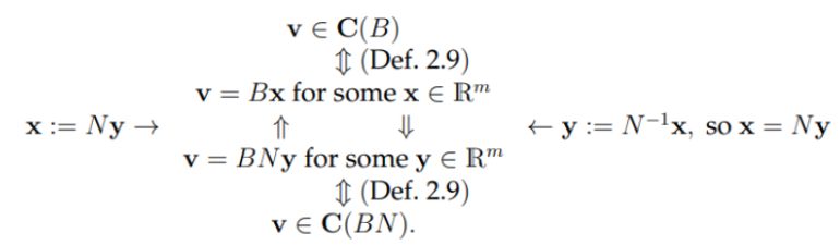
where ! holds because:
Current
Note has been deleted
Field-by-field Comparison
| Field | Before | After |
|---|---|---|
| Front | ||
| Back |
Note 1543: ETH::1. Semester::LinAlg
Deck: ETH::1. Semester::LinAlg
Note Type: Horvath Cloze
GUID:
deleted
Note Type: Horvath Cloze
GUID:
z[vF=azkGx
Deleted Note
Front
The inverse matrix is unique and can be denoted \(A^{-1}\).
Back
The inverse matrix is unique and can be denoted \(A^{-1}\).
Current
Note has been deleted
Field-by-field Comparison
| Field | Before | After |
|---|---|---|
| Text |
Note 1544: ETH::1. Semester::LinAlg
Deck: ETH::1. Semester::LinAlg
Note Type: Horvath Cloze
GUID:
deleted
Note Type: Horvath Cloze
GUID:
zh2KTU;saW
Deleted Note
Front
A matrix \(Q \in \mathbb{R}^{n \times n}\) is orthogonal when \(Q^\top Q = I\).
Back
A matrix \(Q \in \mathbb{R}^{n \times n}\) is orthogonal when \(Q^\top Q = I\).
Current
Note has been deleted
Field-by-field Comparison
| Field | Before | After |
|---|---|---|
| Text |
Note 1545: ETH::1. Semester::LinAlg
Deck: ETH::1. Semester::LinAlg
Note Type: Horvath Cloze
GUID:
deleted
Note Type: Horvath Cloze
GUID:
zz.w6i^0.V
Deleted Note
Front
A matrix \(A \in \mathbb{R}^{n \times n}\) is invertible if and only if \[ \det(A) \neq 0 \]
Back
A matrix \(A \in \mathbb{R}^{n \times n}\) is invertible if and only if \[ \det(A) \neq 0 \]
If the unit cube collapses to have 0 volume (i.e. \(\det(A) = 0\)) then we lost a dimension and \(A\) cannot be invertible.
Current
Note has been deleted
Field-by-field Comparison
| Field | Before | After |
|---|---|---|
| Text | ||
| Extra |
Note 1546: ETH::1. Semester::LinAlg
Deck: ETH::1. Semester::LinAlg
Note Type: Horvath Classic
GUID:
deleted
Note Type: Horvath Classic
GUID:
z{mV]q!JSS
Deleted Note
Front
How do we find the matrix \(A\) associated with a linear transformation \(T_A\)?
Back
How do we find the matrix \(A\) associated with a linear transformation \(T_A\)?
For \(e_1, e_2, \dots, e_n\) we calculate \(T_A(e_k)\) to find the \(k\)-th column of \(A\): \[ A = \begin{bmatrix} | & | & \text{} & | \\ T(e_1) & T(e_2) & \dots & T(e_n) \\ | & | & \text{ } & | \end{bmatrix} \]
Current
Note has been deleted
Field-by-field Comparison
| Field | Before | After |
|---|---|---|
| Front | ||
| Back |
Note 1547: ETH::1. Semester::LinAlg
Deck: ETH::1. Semester::LinAlg
Note Type: Horvath Cloze
GUID:
deleted
Note Type: Horvath Cloze
GUID:
z~{N,b0:-A
Deleted Note
Front
The independent columns of \(A\), {{c1::span the column space \(\textbf{C}(A)\) of \(A\)}}.
Back
The independent columns of \(A\), {{c1::span the column space \(\textbf{C}(A)\) of \(A\)}}.
Proven by induction, adding elements that are a linear combination of other ones doesn't change span, thus we can iteratively remove the dependent columns.
Lemma 2.11
Lemma 2.11
Current
Note has been deleted
Field-by-field Comparison
| Field | Before | After |
|---|---|---|
| Text | ||
| Extra |
Note 1548: ETH::1. Semester::LinAlg
Deck: ETH::1. Semester::LinAlg
Note Type: Horvath Cloze
GUID:
deleted
Note Type: Horvath Cloze
GUID:
}ovjsBoRZ
Deleted Note
Front
Let \(V\) be a vector space. A subset \(B \subseteq V\) is called a basis of \(V\) if
- \(B\) is linearly independent
- {{c1::\(\textbf{Span}(B) = V\).}}
Back
Let \(V\) be a vector space. A subset \(B \subseteq V\) is called a basis of \(V\) if
- \(B\) is linearly independent
- {{c1::\(\textbf{Span}(B) = V\).}}
Current
Note has been deleted
Field-by-field Comparison
| Field | Before | After |
|---|---|---|
| Text |
Note 1549: ETH::1. Semester::A&D
Deck: ETH::1. Semester::A&D
Note Type: Horvath Cloze
GUID:
added
Note Type: Horvath Cloze
GUID:
A!-/#G=){
Previous
Note did not exist
New Note
Front
\(g \geq \Omega(f)\) \( \Leftrightarrow\) \( f \leq O(g)\)
Back
\(g \geq \Omega(f)\) \( \Leftrightarrow\) \( f \leq O(g)\)
Field-by-field Comparison
| Field | Before | After |
|---|---|---|
| Text | {{c2::\(g \geq \Omega(f)\)}} \( \Leftrightarrow\) {{c1::\( f \leq O(g)\)}} |
Note 1550: ETH::1. Semester::A&D
Deck: ETH::1. Semester::A&D
Note Type: Horvath Cloze
GUID:
added
Note Type: Horvath Cloze
GUID:
A+lafWP/s]
Previous
Note did not exist
New Note
Front
In a directed graph we call a (\(\epsilon\)/Eulerian/Hamiltonian) walk/closed walk/path/cycle a directed (gerichtet) (\(\epsilon\)/Eulerian/Hamiltonian) walk/closed walk/path/cycle.
Back
In a directed graph we call a (\(\epsilon\)/Eulerian/Hamiltonian) walk/closed walk/path/cycle a directed (gerichtet) (\(\epsilon\)/Eulerian/Hamiltonian) walk/closed walk/path/cycle.
Field-by-field Comparison
| Field | Before | After |
|---|---|---|
| Text | In a directed graph we call a (\(\epsilon\)/Eulerian/Hamiltonian) walk/closed walk/path/cycle a {{c1::directed (<i>gerichtet</i>)}} (\(\epsilon\)/Eulerian/Hamiltonian) walk/closed walk/path/cycle. |
Note 1551: ETH::1. Semester::A&D
Deck: ETH::1. Semester::A&D
Note Type: Horvath Reverso
GUID:
added
Note Type: Horvath Reverso
GUID:
A1y[0:/g)f
Previous
Note did not exist
New Note
Front
Closed Walk
Back
Closed Walk
Zyklus
Field-by-field Comparison
| Field | Before | After |
|---|---|---|
| Front | Closed Walk | |
| Back | Zyklus |
Note 1552: ETH::1. Semester::A&D
Deck: ETH::1. Semester::A&D
Note Type: Horvath Classic
GUID:
added
Note Type: Horvath Classic
GUID:
A8P;P^G,v4
Previous
Note did not exist
New Note
Front
Runtime of sorting an array containing only \(1, 0\)?
Back
Runtime of sorting an array containing only \(1, 0\)?
Using bucketsort, we can achieve \(O(n)\).
We go through the array once, counting occurences of \(0\) as x. We then add \(x\) zeros in the beginning and fill the rest with 1s.
We go through the array once, counting occurences of \(0\) as x. We then add \(x\) zeros in the beginning and fill the rest with 1s.
Field-by-field Comparison
| Field | Before | After |
|---|---|---|
| Front | Runtime of sorting an array containing only \(1, 0\)? | |
| Back | Using bucketsort, we can achieve \(O(n)\). <br><br>We go through the array once, counting occurences of \(0\) as x. We then add \(x\) zeros in the beginning and fill the rest with 1s. |
Note 1553: ETH::1. Semester::A&D
Deck: ETH::1. Semester::A&D
Note Type: Algorithms
GUID:
added
Note Type: Algorithms
GUID:
AJT5T7qaW3
Previous
Note did not exist
New Note
Front
Runtime of Find Closed Eulerian Path?
Back
Runtime of Find Closed Eulerian Path?
\(O(n+m)\)
In an Adjacency Matrix: runtime is \(O(n^2)\) as looping over all edges is \(O(n)\).
In an Adjacency List: we loop \(n\) times over \(O(1 + \deg(u))\).
Using the handshake lemma: \(\sum_{u \in V} (1 + \deg(u)) = n + \sum_{u \in V} \deg(u) = n + 2m\)
In an Adjacency Matrix: runtime is \(O(n^2)\) as looping over all edges is \(O(n)\).
In an Adjacency List: we loop \(n\) times over \(O(1 + \deg(u))\).
Using the handshake lemma: \(\sum_{u \in V} (1 + \deg(u)) = n + \sum_{u \in V} \deg(u) = n + 2m\)
Field-by-field Comparison
| Field | Before | After |
|---|---|---|
| Name | Find Closed Eulerian Path | |
| Runtime | \(O(n+m)\) | |
| Approach | We want to be able to find closed walks in a graph. We can then merge them together to form a single closed walk, by exploiting shared vertices.<br><br>Algo:<br><ol><li>Start at vertex \(u_0\) arbitrary</li><li>For loop over edges. If not marked, mark and recurse.</li><li>Append vertex to list after execution</li></ol> Returns a list of vertices in order of a closed walk if there is one.<br><br>Example:<br><img src="paste-a669de30c7bc4a38d788fb96b6b5551a4781ec71.jpg"><br>Output:<br><img src="paste-b453826818903aa4da2ac10897e9dc0e177229b6.jpg"> | |
| Pseudocode | <img src="paste-b2cbbb1cb599a09a77bcc0e991ec4bcb83c586fb.jpg"><br><img src="paste-c82a6519899f9b1f1f49c932a2b252ff64a2184a.jpg"> | |
| Extra Info | In an Adjacency Matrix: runtime is \(O(n^2)\) as looping over all edges is \(O(n)\).<br><br>In an Adjacency List: we loop \(n\) times over \(O(1 + \deg(u))\).<br>Using the handshake lemma: \(\sum_{u \in V} (1 + \deg(u)) = n + \sum_{u \in V} \deg(u) = n + 2m\) |
Note 1554: ETH::1. Semester::A&D
Deck: ETH::1. Semester::A&D
Note Type: Horvath Cloze
GUID:
added
Note Type: Horvath Cloze
GUID:
AQQfmx,sQF
Previous
Note did not exist
New Note
Front
A graph \(G\) is acyclic (azyklisch) if it has no cycles (Kreise).
Back
A graph \(G\) is acyclic (azyklisch) if it has no cycles (Kreise).
Field-by-field Comparison
| Field | Before | After |
|---|---|---|
| Text | A graph \(G\) is {{c1::acyclic (<i>azyklisch</i>)}} if it {{c2::has no cycles (<i>Kreise</i>)}}. |
Note 1555: ETH::1. Semester::A&D
Deck: ETH::1. Semester::A&D
Note Type: Horvath Cloze
GUID:
added
Note Type: Horvath Cloze
GUID:
AS{7LiImd:
Previous
Note did not exist
New Note
Front
A graph \(G\) is bipartite if {{c2:: it's possible to partition the vertices into two sets \(V_1\) and \(V_2\) that are disjoint and cover the graph. Any edge \(\{u, v\}\) has to have one endpoint in \(V_1\) and the other in \(V_2\)}}.
Back
A graph \(G\) is bipartite if {{c2:: it's possible to partition the vertices into two sets \(V_1\) and \(V_2\) that are disjoint and cover the graph. Any edge \(\{u, v\}\) has to have one endpoint in \(V_1\) and the other in \(V_2\)}}.
Field-by-field Comparison
| Field | Before | After |
|---|---|---|
| Text | A graph \(G\) is {{c1::<b>bipartite</b>}} if {{c2:: it's possible to partition the vertices into two sets \(V_1\) and \(V_2\) that are disjoint and cover the graph. Any edge \(\{u, v\}\) has to have one endpoint in \(V_1\) and the other in \(V_2\)}}. |
Note 1556: ETH::1. Semester::A&D
Deck: ETH::1. Semester::A&D
Note Type: Horvath Cloze
GUID:
added
Note Type: Horvath Cloze
GUID:
AY}!l[d)1z
Previous
Note did not exist
New Note
Front
Name the impossible cases in DFS pre/post ordering for edge \((u, v)\):
- Overlapping but not nested intervals:
- {{c2:: \(\text{pre}(u)<\text{pre}(v)<\text{post}(u)<\text{post}(v)\): As visit(u) would call visit(v) before the recursive call ends. }}
Back
Name the impossible cases in DFS pre/post ordering for edge \((u, v)\):
- Overlapping but not nested intervals:
- {{c2:: \(\text{pre}(u)<\text{pre}(v)<\text{post}(u)<\text{post}(v)\): As visit(u) would call visit(v) before the recursive call ends. }}
Field-by-field Comparison
| Field | Before | After |
|---|---|---|
| Text | Name the impossible cases in DFS pre/post ordering for edge \((u, v)\):<br><ul><li>{{c1::Overlapping but not nested intervals: <img src="paste-b7976dbbff12de2b44594553e0c91633f59e9c05.jpg">}}</li><li>{{c2:: \(\text{pre}(u)<\text{pre}(v)<\text{post}(u)<\text{post}(v)\): As visit(u) would call visit(v) before the recursive call ends. <img src="paste-a6fc070f96de8bd2b8148e3891cf956fd611a0a2.jpg"> }}</li></ul> |
Note 1557: ETH::1. Semester::A&D
Deck: ETH::1. Semester::A&D
Note Type: Algorithms
GUID:
added
Note Type: Algorithms
GUID:
Ah4U@kYYNJ
Previous
Note did not exist
New Note
Front
Runtime of Linear Search?
Back
Runtime of Linear Search?
\(\Theta(n)\) as we go through the entire list once.
Field-by-field Comparison
| Field | Before | After |
|---|---|---|
| Name | Linear Search | |
| Runtime | \(\Theta(n)\) as we go through the entire list once. | |
| Requirements | Linear search does <i>not</i> require a sorted array, it will perform the same on any array. | |
| Approach | Go through the entire list and compare the current element to the one we are looking for. |
Note 1558: ETH::1. Semester::A&D
Deck: ETH::1. Semester::A&D
Note Type: Horvath Cloze
GUID:
added
Note Type: Horvath Cloze
GUID:
Ah6X9iA&#j
Previous
Note did not exist
New Note
Front
The ADT stack has the following operations:
- push(k, S): push a new object k to the top of the stack S
- pop(S): remove and return the top element of the stack S
- top(S): get the top element of the stack S without deleting it
Back
The ADT stack has the following operations:
- push(k, S): push a new object k to the top of the stack S
- pop(S): remove and return the top element of the stack S
- top(S): get the top element of the stack S without deleting it
Other operations might be isEmpty or emptystack which produces and emtpy stack.
Field-by-field Comparison
| Field | Before | After |
|---|---|---|
| Text | The ADT <b>stack</b> has the following operations:<br><ul><li><b>push(k, S)</b>: {{c1:: push a new object <b>k</b> to the top of the stack <b>S</b>}}</li><li><b>pop(S)</b>: {{c2:: remove and return the top element of the stack <b>S</b>}}</li><li><b>top(S)</b>: {{c3:: get the top element of the stack <b>S</b> without deleting it}}</li></ul> | |
| Extra | Other operations might be <b>isEmpty</b> or <b>emptystack</b> which produces and emtpy stack. |
Note 1559: ETH::1. Semester::A&D
Deck: ETH::1. Semester::A&D
Note Type: Horvath Classic
GUID:
added
Note Type: Horvath Classic
GUID:
AqQ}Ty8GRj
Previous
Note did not exist
New Note
Front
How do we fix the Quicksort worst-case runtime?
Back
How do we fix the Quicksort worst-case runtime?
Chose a random element as the pivot.
Median of medians algo ideal but too complex to implement.
Median of medians algo ideal but too complex to implement.
Field-by-field Comparison
| Field | Before | After |
|---|---|---|
| Front | How do we fix the Quicksort worst-case runtime? | |
| Back | Chose a random element as the pivot.<br><br>Median of medians algo ideal but too complex to implement. |
Note 1560: ETH::1. Semester::A&D
Deck: ETH::1. Semester::A&D
Note Type: Horvath Cloze
GUID:
added
Note Type: Horvath Cloze
GUID:
Au,kdh[/@(
Previous
Note did not exist
New Note
Front
A safe edge is an edge that is included in at all MSTs.
Back
A safe edge is an edge that is included in at all MSTs.
all, If the edge-weights are distinct, which means there is one unique MST.
Field-by-field Comparison
| Field | Before | After |
|---|---|---|
| Text | A {{c1::<b>safe edge</b>}} is an {{c2:: edge that is included in at <i>all</i> MSTs}}. | |
| Extra | <div><i>all, </i>If the edge-weights are distinct, which means there is one unique MST.</div> |
Note 1561: ETH::1. Semester::A&D
Deck: ETH::1. Semester::A&D
Note Type: Horvath Cloze
GUID:
added
Note Type: Horvath Cloze
GUID:
Auw]yKf@xT
Previous
Note did not exist
New Note
Front
Pre-/Post-Ordering Classification for an edge \((u, v)\):
\(\text{pre}(u) < \text{pre}(v) < \text{post}(v) < \text{post}(u)\), but not tree edge: Forward edge
\(\text{pre}(u) < \text{pre}(v) < \text{post}(v) < \text{post}(u)\), but not tree edge: Forward edge
Back
Pre-/Post-Ordering Classification for an edge \((u, v)\):
\(\text{pre}(u) < \text{pre}(v) < \text{post}(v) < \text{post}(u)\), but not tree edge: Forward edge
\(\text{pre}(u) < \text{pre}(v) < \text{post}(v) < \text{post}(u)\), but not tree edge: Forward edge
Field-by-field Comparison
| Field | Before | After |
|---|---|---|
| Text | Pre-/Post-Ordering Classification for an edge \((u, v)\):<br><br>\(\text{pre}(u) < \text{pre}(v) < \text{post}(v) < \text{post}(u)\), but <b>not tree edge</b>: {{c1:: Forward edge}} |
Note 1562: ETH::1. Semester::A&D
Deck: ETH::1. Semester::A&D
Note Type: Horvath Classic
GUID:
added
Note Type: Horvath Classic
GUID:
B#Jj9:E=8j
Previous
Note did not exist
New Note
Front
Cut and Paste Proof of Cut-Property:
Back
Cut and Paste Proof of Cut-Property:
Let \((S, V \setminus S)\) be any cut of a graph \(G\).
Let \(e = (u,v)\) be the minimal edge crossing this cut.
We want to show that \(e \in T\).
- Assume \(e \not \in T\) for contradiction.
- Since \(T\) is a spanning tree, \(T \cup {u}\) contains a cycle, crossing the cut at least twice (once via \(e\) and once via another edge \(e’\).)
- We now construct \(T’= (T \cup {e}) \setminus {e’}\) which breaks the cycle but keeps the MST property.
- Since \(w(e) < w(e’)\), \(w(T’) < w(T)\) and thus \(T\) is not an MST.
Field-by-field Comparison
| Field | Before | After |
|---|---|---|
| Front | Cut and Paste Proof of <b>Cut-Property</b>: | |
| Back | <div>Let \((S, V \setminus S)\) be any cut of a graph \(G\).</div><div><br></div><div>Let \(e = (u,v)\) be the minimal edge crossing this cut. </div><div>We want to show that \(e \in T\). </div><div><br></div><div><ol><li>Assume \(e \not \in T\) for contradiction.</li><li>Since \(T\) is a spanning tree, \(T \cup {u}\) contains a cycle, crossing the cut at least twice (once via \(e\) and once via another edge \(e’\).)</li><li>We now construct \(T’= (T \cup {e}) \setminus {e’}\) which breaks the cycle but keeps the MST property.</li><li>Since \(w(e) < w(e’)\), \(w(T’) < w(T)\) and thus \(T\) is not an MST.</li></ol></div> |
Note 1563: ETH::1. Semester::A&D
Deck: ETH::1. Semester::A&D
Note Type: Horvath Classic
GUID:
added
Note Type: Horvath Classic
GUID:
B)ghZbgf?6
Previous
Note did not exist
New Note
Front
Describe the steps of Prim's Algorithm:
Back
Describe the steps of Prim's Algorithm:
Prim’s algorithm starts with a single vertex and grows the MST outwards from that seed.
- Initialisation:
- Select and arbitrary starting vertex \(s\) and empty set \(F\)
- Set \(S = {s}\) tracks the vertices in the MST
- Each vertex gets a
key[v] =representing the cheapest known connection cost to \(v\):- \(\infty\) if no edge connects \(s\) to \(v\)
- \(w(s, v)\) if edge \((s, v)\) exists
- Use a priority queue \(Q\) (Min-Heap) to store the vertices, in order of lowest
keycost
- Iteration:
- Select and add Extract the vertex \(u\) with the minimum
keyfrom \(Q\). This is the cheapest to connected to the current MST. Add \(u\) to \(S\). - Update Neighbours For each neighbour \(v\) of \(u\) not in \(S\):
- If \(w(u, v) < \text{key}[v]\) update
key[v] = w(u, v)and update the priority in $Q$.- This discovers potentially cheaper connections to vertices outside the current MST. If a cheaper edge to \(v\) is found, the current value in
key[v]cannot be part of the MST
- This discovers potentially cheaper connections to vertices outside the current MST. If a cheaper edge to \(v\) is found, the current value in
- If \(w(u, v) < \text{key}[v]\) update
- Select and add Extract the vertex \(u\) with the minimum
- Termination: When \(Q\) is empty, all vertices are in \(S\) and connected, and the edges chosen are in the MST (tracked in the set \(F\) through updates).
Field-by-field Comparison
| Field | Before | After |
|---|---|---|
| Front | Describe the steps of <b>Prim's Algorithm</b>: | |
| Back | <div>Prim’s algorithm starts with a single vertex and grows the MST outwards from that seed.</div> <ol> <li><strong>Initialisation:</strong><ul> <li>Select and arbitrary starting vertex \(s\) and empty set \(F\)</li> <li>Set \(S = {s}\) tracks the vertices in the MST</li> <li>Each vertex gets a <code>key[v] =</code> representing the cheapest known connection cost to \(v\):<ul> <li>\(\infty\) if no edge connects \(s\) to \(v\)</li> <li>\(w(s, v)\) if edge \((s, v)\) exists</li> </ul> </li> <li>Use a priority queue \(Q\) (<em>Min-Heap</em>) to store the vertices, in order of lowest <code>key</code> cost</li> </ul> </li> <li><strong>Iteration:</strong><ul> <li><em>Select and add</em> Extract the vertex \(u\) with the minimum <code>key</code> from \(Q\). This is the cheapest to connected to the current MST. Add \(u\) to \(S\).</li> <li><em>Update Neighbours</em> For each neighbour <b>\(v\) </b>of \(u\) <em>not</em> in \(S\):<ul> <li>If \(w(u, v) < \text{key}[v]\) update <code>key[v] = w(u, v)</code> and update the priority in $Q$.<ul> <li>This discovers potentially cheaper connections to vertices outside the current MST. If a <em>cheaper edge</em> to \(v\) is found, the current value in <code>key[v]</code> cannot be part of the MST</li> </ul> </li> </ul> </li> </ul> </li> <li><strong>Termination:</strong> When \(Q\) is empty, all vertices are in \(S\) and connected, and the edges chosen are in the MST (tracked in the set \(F\) through updates).</li></ol> |
Note 1564: ETH::1. Semester::A&D
Deck: ETH::1. Semester::A&D
Note Type: Horvath Reverso
GUID:
added
Note Type: Horvath Reverso
GUID:
B+m&Yt;~bM
Previous
Note did not exist
New Note
Front
Path
Back
Path
Pfad
Field-by-field Comparison
| Field | Before | After |
|---|---|---|
| Front | Path | |
| Back | Pfad |
Note 1565: ETH::1. Semester::A&D
Deck: ETH::1. Semester::A&D
Note Type: Horvath Cloze
GUID:
added
Note Type: Horvath Cloze
GUID:
B/7aNL0zYE
Previous
Note did not exist
New Note
Front
Boruvka's Algorithm has a runtime of \(O((|V| + |E|) \log |V|)\).
Back
Boruvka's Algorithm has a runtime of \(O((|V| + |E|) \log |V|)\).
During each iteration, we examine all edges to find the cheapest one: \(O(|V| + |E|)\):
- Run DFS to find the connected components: \(O(|V| + |E|)\)
- Find the cheapest one \(O(|E|)\)
Field-by-field Comparison
| Field | Before | After |
|---|---|---|
| Text | <b>Boruvka's Algorithm</b> has a runtime of {{c1:: \(O((|V| + |E|) \log |V|)\)}}. | |
| Extra | During each iteration, we examine all edges to find the cheapest one: \(O(|V| + |E|)\):<br><ol><li>Run DFS to find the connected components: \(O(|V| + |E|)\)</li><li>Find the cheapest one \(O(|E|)\)</li></ol>We iterate a total of \(\log_2 |V|\) times as each iteration halves the number of connected components. |
Note 1566: ETH::1. Semester::A&D
Deck: ETH::1. Semester::A&D
Note Type: Horvath Cloze
GUID:
added
Note Type: Horvath Cloze
GUID:
B9BorfLC*u
Previous
Note did not exist
New Note
Front
{{c1:: \(\sum_{i = 1}^{n} i\)::Sum}} \(\leq\) \(O(n^2)\)
Back
{{c1:: \(\sum_{i = 1}^{n} i\)::Sum}} \(\leq\) \(O(n^2)\)
Field-by-field Comparison
| Field | Before | After |
|---|---|---|
| Text | {{c1:: \(\sum_{i = 1}^{n} i\)::Sum}} \(\leq\) {{c2::\(O(n^2)\)}} |
Note 1567: ETH::1. Semester::A&D
Deck: ETH::1. Semester::A&D
Note Type: Algorithms
GUID:
added
Note Type: Algorithms
GUID:
BRmyi3>lm%
Previous
Note did not exist
New Note
Front
Back
Runtime of
DFS
Runtime: {{c1::\( \mathcal{O}(|E| + |V|) \)}}
Approach:
Uses:
?Field-by-field Comparison
| Field | Before | After |
|---|---|---|
| Name | <div style="text-align: center;"><b>DFS</b></div><div><br></div><div><b>Runtime</b>: {{c1::\( \mathcal{O}(|E| + |V|) \)}}</div><div><br></div><div><b>Approach</b>: {{c2::Explore as far as possible along each branch before backtracking. Potentially keep track of pre- / post-numbers to make edge classifications.}}</div><div><br></div><div><b>Uses</b>: {{c3::Detect cycles (if backward edge), <b>topological sorting </b>(reverse post-ordering), test if bipartite, mazes, ...}}</div> |
Note 1568: ETH::1. Semester::A&D
Deck: ETH::1. Semester::A&D
Note Type: Horvath Cloze
GUID:
added
Note Type: Horvath Cloze
GUID:
Bb-m%-jtI|
Previous
Note did not exist
New Note
Front
Pre-/Post-Ordering Classification for an edge \((u, v)\):
\(\text{pre}(v) < \text{post}(v) < \text{pre}(u) < \text{post}(u)\): Cross edge, \(u, v\) in different subtrees
\(\text{pre}(v) < \text{post}(v) < \text{pre}(u) < \text{post}(u)\): Cross edge, \(u, v\) in different subtrees
Back
Pre-/Post-Ordering Classification for an edge \((u, v)\):
\(\text{pre}(v) < \text{post}(v) < \text{pre}(u) < \text{post}(u)\): Cross edge, \(u, v\) in different subtrees
\(\text{pre}(v) < \text{post}(v) < \text{pre}(u) < \text{post}(u)\): Cross edge, \(u, v\) in different subtrees
Field-by-field Comparison
| Field | Before | After |
|---|---|---|
| Text | Pre-/Post-Ordering Classification for an edge \((u, v)\):<br><br>\(\text{pre}(v) < \text{post}(v) < \text{pre}(u) < \text{post}(u)\): {{c1:: Cross edge, \(u, v\) in different subtrees}} |
Note 1569: ETH::1. Semester::A&D
Deck: ETH::1. Semester::A&D
Note Type: Horvath Cloze
GUID:
added
Note Type: Horvath Cloze
GUID:
Bgd/GP4-Fq
Previous
Note did not exist
New Note
Front
A graph \(G\) is a tree if it is connected and has no cycles (Kreise).
Back
A graph \(G\) is a tree if it is connected and has no cycles (Kreise).
Field-by-field Comparison
| Field | Before | After |
|---|---|---|
| Text | A graph \(G\) is a {{c1::tree}} if it is {{c2::connected and has no cycles (<i>Kreise</i>)}}. |
Note 1570: ETH::1. Semester::A&D
Deck: ETH::1. Semester::A&D
Note Type: Horvath Classic
GUID:
added
Note Type: Horvath Classic
GUID:
Bq5(?)1v6(
Previous
Note did not exist
New Note
Front
What does \(\prod_{i=1}^n a_i\) mean?
Back
What does \(\prod_{i=1}^n a_i\) mean?
it is the product of all numbers between \(i\) and \(n\), in this specific case it is \(n!\)
Field-by-field Comparison
| Field | Before | After |
|---|---|---|
| Front | What does \(\prod_{i=1}^n a_i\) mean? | |
| Back | it is the product of all numbers between \(i\) and \(n\), in this specific case it is \(n!\) |
Note 1571: ETH::1. Semester::A&D
Deck: ETH::1. Semester::A&D
Note Type: Horvath Cloze
GUID:
added
Note Type: Horvath Cloze
GUID:
Br&58pkCU{
Previous
Note did not exist
New Note
Front
We start counting the height of a tree at \(0\).
Back
We start counting the height of a tree at \(0\).
Field-by-field Comparison
| Field | Before | After |
|---|---|---|
| Text | We start counting the height of a tree at {{c1::\(0\)}}. |
Note 1572: ETH::1. Semester::A&D
Deck: ETH::1. Semester::A&D
Note Type: Horvath Cloze
GUID:
added
Note Type: Horvath Cloze
GUID:
BvQCv]T&c0
Previous
Note did not exist
New Note
Front
Choose a tight bound!
\(O(\log(n!))\leq O(n \log(n))\)
\(O(\log(n!))\leq O(n \log(n))\)
Back
Choose a tight bound!
\(O(\log(n!))\leq O(n \log(n))\)
\(O(\log(n!))\leq O(n \log(n))\)
Field-by-field Comparison
| Field | Before | After |
|---|---|---|
| Text | Choose a tight bound!<br><br>\({{c1::O(\log(n!))}}\leq {{c2::O(n \log(n))}}\) |
Note 1573: ETH::1. Semester::A&D
Deck: ETH::1. Semester::A&D
Note Type: Horvath Cloze
GUID:
added
Note Type: Horvath Cloze
GUID:
BwR)%}KG6h
Previous
Note did not exist
New Note
Front
Boruvka's Algorithm requires an undirected, connected, weighted Graph.
Back
Boruvka's Algorithm requires an undirected, connected, weighted Graph.
Field-by-field Comparison
| Field | Before | After |
|---|---|---|
| Text | <b>Boruvka's Algorithm</b> requires an {{c1:: undirected, connected, weighted}} Graph. |
Note 1574: ETH::1. Semester::A&D
Deck: ETH::1. Semester::A&D
Note Type: Horvath Cloze
GUID:
added
Note Type: Horvath Cloze
GUID:
Bz)mOB:[n-
Previous
Note did not exist
New Note
Front
2-3 Tree: The runtime of search, insertion and deletion is \(O(\log n)\).
Back
2-3 Tree: The runtime of search, insertion and deletion is \(O(\log n)\).
This is because the tree is now forced to be balanced and \(h \leq \log_2 n\).
Field-by-field Comparison
| Field | Before | After |
|---|---|---|
| Text | <b>2-3 Tree</b>: The runtime of search, insertion and deletion is{{c1:: \(O(\log n)\)}}. | |
| Extra | This is because the tree is now forced to be balanced and \(h \leq \log_2 n\). |
Note 1575: ETH::1. Semester::A&D
Deck: ETH::1. Semester::A&D
Note Type: Algorithms
GUID:
added
Note Type: Algorithms
GUID:
C$#TvbwG_l
Previous
Note did not exist
New Note
Front
Runtime of Longest Ascending Subsequence (Längste Aufsteigende Teilfolge)?
Back
Runtime of Longest Ascending Subsequence (Längste Aufsteigende Teilfolge)?
\(\Theta(n \log n)\)
Field-by-field Comparison
| Field | Before | After |
|---|---|---|
| Name | Longest Ascending Subsequence (Längste Aufsteigende Teilfolge) | |
| Runtime | \(\Theta(n \log n)\) | |
| Approach | For an array A[1..n] <b>longest</b> subsequence (non-continuous) that is ascending.<br><br>DP Table with entry \(M(l) = a\) where a ist the smallest possible ending of a LAT with length \(l\).<br><ul><li>Base Cases: \(M[*] = \infty\)</li><li>Recursion: set \(M[k]\) to \(A[i]\) where \(k\) is the index of the next smallest + 1 in \(M\).</li></ul>We can find the smaller with binary search, thus \(\log n \) search for \(n\) elements -> \(\Theta(n \log n)\).<br><img src="paste-1b9069bf0a881a3cd3900a4de699cac89f0498b8.jpg"><br> | |
| Pseudocode | <img src="paste-0cd3692a4a909acf7f7ae0540eb6d714fc346b41.jpg"> |
Note 1576: ETH::1. Semester::A&D
Deck: ETH::1. Semester::A&D
Note Type: Horvath Cloze
GUID:
added
Note Type: Horvath Cloze
GUID:
C1$vvwFoR0
Previous
Note did not exist
New Note
Front
In graph theory, a closed Eulerian walk (Eulerzyklus) is an Eulerian walk (Eulerweg) that ends at the start vertex.
Back
In graph theory, a closed Eulerian walk (Eulerzyklus) is an Eulerian walk (Eulerweg) that ends at the start vertex.
Field-by-field Comparison
| Field | Before | After |
|---|---|---|
| Text | In graph theory, a {{c2::closed Eulerian walk (Eulerzyklus)}} is an {{c1::Eulerian walk (Eulerweg) that ends at the start vertex}}. |
Note 1577: ETH::1. Semester::A&D
Deck: ETH::1. Semester::A&D
Note Type: Horvath Classic
GUID:
added
Note Type: Horvath Classic
GUID:
C5BRbDI3JL
Previous
Note did not exist
New Note
Front
j = 1
while j <= n do
j = 2j
f()
Back
j = 1
while j <= n do
j = 2j
f()
\[\sum_{j = 0}^{\lfloor \log_2 n \rfloor}\]
We go from \(0\) to \(\lfloor \log_2 n \rfloor\) not from \(1\).
Field-by-field Comparison
| Field | Before | After |
|---|---|---|
| Front | <pre><code>j = 1 while j <= n do j = 2j f()<br></code></pre> Sum form of exact calls of f()? | |
| Back | <div></div><div>\[\sum_{j = 0}^{\lfloor \log_2 n \rfloor}\]</div><div>We go from \(0\) to \(\lfloor \log_2 n \rfloor\) not from \(1\).</div> |
Note 1578: ETH::1. Semester::A&D
Deck: ETH::1. Semester::A&D
Note Type: Horvath Cloze
GUID:
added
Note Type: Horvath Cloze
GUID:
C9v-$JhadV
Previous
Note did not exist
New Note
Front
If \(\frac{f(n)}{g(n)}\) tends to 0, then \(f \leq O(g)\) and \(f \neq \Theta(g)\)
Back
If \(\frac{f(n)}{g(n)}\) tends to 0, then \(f \leq O(g)\) and \(f \neq \Theta(g)\)
Field-by-field Comparison
| Field | Before | After |
|---|---|---|
| Text | If \(\frac{f(n)}{g(n)}\) tends to {{c1:: 0}}, then {{c2::\(f \leq O(g)\) and \(f \neq \Theta(g)\)}} |
Note 1579: ETH::1. Semester::A&D
Deck: ETH::1. Semester::A&D
Note Type: Horvath Classic
GUID:
added
Note Type: Horvath Classic
GUID:
CJsa&>C5sO
Previous
Note did not exist
New Note
Front
Can Kruskal's Algorithm be executed in \(O(|E| + |V|\log|V|)\) time?
Back
Can Kruskal's Algorithm be executed in \(O(|E| + |V|\log|V|)\) time?
No, we need to sort the edges which takes at least \(|E| \log |E|\) time.
Field-by-field Comparison
| Field | Before | After |
|---|---|---|
| Front | Can Kruskal's Algorithm be executed in \(O(|E| + |V|\log|V|)\) time? | |
| Back | No, we need to sort the edges which takes at least \(|E| \log |E|\) time. |
Note 1580: ETH::1. Semester::A&D
Deck: ETH::1. Semester::A&D
Note Type: Horvath Cloze
GUID:
added
Note Type: Horvath Cloze
GUID:
CaRvZ82Z-e
Previous
Note did not exist
New Note
Front
{{c1:: \(\sum_{i = 1}^{n} \sum_{i = 1}^{n} \sum_{i = 1}^{n} 1\)::Sum}} \(=\) \(n^3\)
Back
{{c1:: \(\sum_{i = 1}^{n} \sum_{i = 1}^{n} \sum_{i = 1}^{n} 1\)::Sum}} \(=\) \(n^3\)
Field-by-field Comparison
| Field | Before | After |
|---|---|---|
| Text | {{c1:: \(\sum_{i = 1}^{n} \sum_{i = 1}^{n} \sum_{i = 1}^{n} 1\)::Sum}} \(=\) {{c2:: \(n^3\)}} |
Note 1581: ETH::1. Semester::A&D
Deck: ETH::1. Semester::A&D
Note Type: Horvath Cloze
GUID:
added
Note Type: Horvath Cloze
GUID:
Ceyt5d#^?A
Previous
Note did not exist
New Note
Front
\( g = \Theta(f)\) \(\Leftrightarrow\) {{c1:: \(g \leq O(f) \text{ and } f \leq O(g)\)}}
Back
\( g = \Theta(f)\) \(\Leftrightarrow\) {{c1:: \(g \leq O(f) \text{ and } f \leq O(g)\)}}
Field-by-field Comparison
| Field | Before | After |
|---|---|---|
| Text | {{c2::\( g = \Theta(f)\)}} \(\Leftrightarrow\) {{c1:: \(g \leq O(f) \text{ and } f \leq O(g)\)}} |
Note 1582: ETH::1. Semester::A&D
Deck: ETH::1. Semester::A&D
Note Type: Horvath Classic
GUID:
added
Note Type: Horvath Classic
GUID:
Cnkg?3]K
Previous
Note did not exist
New Note
Front
Quicksort space complexity?
Back
Quicksort space complexity?
\(O(n)\)
Field-by-field Comparison
| Field | Before | After |
|---|---|---|
| Front | Quicksort space complexity? | |
| Back | \(O(n)\) |
Note 1583: ETH::1. Semester::A&D
Deck: ETH::1. Semester::A&D
Note Type: Horvath Classic
GUID:
added
Note Type: Horvath Classic
GUID:
Cz/kys?.PN
Previous
Note did not exist
New Note
Front
Every undirected graph that contains a Hamilton path also contains an eulerian walk?
Back
Every undirected graph that contains a Hamilton path also contains an eulerian walk?
No.
Field-by-field Comparison
| Field | Before | After |
|---|---|---|
| Front | Every undirected graph that contains a Hamilton path also contains an eulerian walk? | |
| Back | No.<br><img alt="" src="paste.png"> |
Note 1584: ETH::1. Semester::A&D
Deck: ETH::1. Semester::A&D
Note Type: Horvath Cloze
GUID:
added
Note Type: Horvath Cloze
GUID:
C}:U@+B*;Q
Previous
Note did not exist
New Note
Front
{{c1:: \(\sum_{i = 1}^{n} i^3\)::Sum}} \(\leq\) \(O(n^4)\)
Back
{{c1:: \(\sum_{i = 1}^{n} i^3\)::Sum}} \(\leq\) \(O(n^4)\)
Field-by-field Comparison
| Field | Before | After |
|---|---|---|
| Text | {{c1:: \(\sum_{i = 1}^{n} i^3\)::Sum}} \(\leq\) {{c2::\(O(n^4)\)}} |
Note 1585: ETH::1. Semester::A&D
Deck: ETH::1. Semester::A&D
Note Type: Horvath Cloze
GUID:
added
Note Type: Horvath Cloze
GUID:
D!4=n6GM2_
Previous
Note did not exist
New Note
Front
In a doubly linked list, we store a pointer to the previous and next element for each key.
This increases memory usage as a trade-off for speed.
This increases memory usage as a trade-off for speed.
Back
In a doubly linked list, we store a pointer to the previous and next element for each key.
This increases memory usage as a trade-off for speed.
This increases memory usage as a trade-off for speed.
Field-by-field Comparison
| Field | Before | After |
|---|---|---|
| Text | In a <b>doubly linked list</b>, we store a pointer to the {{c1:: previous and next element}} for each key.<br><br>This increases {{c2::memory usage}} as a trade-off for {{c2:: speed}}. |
Note 1586: ETH::1. Semester::A&D
Deck: ETH::1. Semester::A&D
Note Type: Horvath Classic
GUID:
added
Note Type: Horvath Classic
GUID:
D%cpEp.*I3
Previous
Note did not exist
New Note
Front
What is l'Hôpital's Rule?
Back
What is l'Hôpital's Rule?
If \(\lim_{x \to \infty} f(x) = \lim_{x \to \infty} g(x) = \infty\) (or both \(=0\)), and \(\lim_{x \to \infty} \frac{f'(x)}{g'(x)}\) exists (or is \(\pm\infty\)), then:
\(\lim_{x \to \infty} \frac{f(x)}{g(x)} = \lim_{x \to \infty} \frac{f'(x)}{g'(x)}\)
Field-by-field Comparison
| Field | Before | After |
|---|---|---|
| Front | What is l'Hôpital's Rule? | |
| Back | <div>If \(\lim_{x \to \infty} f(x) = \lim_{x \to \infty} g(x) = \infty\) (or both \(=0\)), and \(\lim_{x \to \infty} \frac{f'(x)}{g'(x)}\) exists (or is \(\pm\infty\)), then:<br></div><div><br></div> <div>\(\lim_{x \to \infty} \frac{f(x)}{g(x)} = \lim_{x \to \infty} \frac{f'(x)}{g'(x)}\)</div> |
Note 1587: ETH::1. Semester::A&D
Deck: ETH::1. Semester::A&D
Note Type: Horvath Cloze
GUID:
added
Note Type: Horvath Cloze
GUID:
D2>~h
Previous
Note did not exist
New Note
Front
The ADT queue has the following operations:
- enqueue(k, S): append at the end of the queue
- dequeue(S): remove and return the first element of the queue
Back
The ADT queue has the following operations:
- enqueue(k, S): append at the end of the queue
- dequeue(S): remove and return the first element of the queue
Field-by-field Comparison
| Field | Before | After |
|---|---|---|
| Text | The ADT <b>queue</b> has the following operations:<br><ul><li><b>enqueue(k, S)</b>: {{c2:: append at the end of the queue}}</li><li><b>dequeue(S)</b>: {{c4:: remove and return the first element of the queue}}</li></ul> |
Note 1588: ETH::1. Semester::A&D
Deck: ETH::1. Semester::A&D
Note Type: Horvath Cloze
GUID:
added
Note Type: Horvath Cloze
GUID:
D9:.N,D17I
Previous
Note did not exist
New Note
Front
A graph \(G\) is called a directed acyclic graph (DAG) (gerichteter azyklischer Graph) if there is no directed cycles (gerichteter Kreis).
Back
A graph \(G\) is called a directed acyclic graph (DAG) (gerichteter azyklischer Graph) if there is no directed cycles (gerichteter Kreis).
Field-by-field Comparison
| Field | Before | After |
|---|---|---|
| Text | A graph \(G\) is called a {{c1::directed acyclic graph (DAG) (<i>gerichteter azyklischer Graph</i>)}} if there is {{c2::no directed cycles (<i>gerichteter Kreis</i>)}}. |
Note 1589: ETH::1. Semester::A&D
Deck: ETH::1. Semester::A&D
Note Type: Algorithms
GUID:
added
Note Type: Algorithms
GUID:
DD]dBe%Sn|
Previous
Note did not exist
New Note
Front
Runtime of Binary Search?
Back
Runtime of Binary Search?
\(O(\log(n))\) (optimal)
Field-by-field Comparison
| Field | Before | After |
|---|---|---|
| Name | Binary Search | |
| Runtime | \(O(\log(n))\) (optimal) | |
| Requirements | Sorted Array | |
| Approach | Start in the middle of the array. <br><br>If the middle element is the target element, return the current index.<br><br>Else if the middle elment is larger (smaller) than the target element, continue recursively on the left (right) half of the array. | |
| Pseudocode | <img src="paste-c63669116a3e862cbe19f556da7b184c6cecc888.jpg"> |
Note 1590: ETH::1. Semester::A&D
Deck: ETH::1. Semester::A&D
Note Type: Horvath Classic
GUID:
added
Note Type: Horvath Classic
GUID:
D]]~[I)jx9
Previous
Note did not exist
New Note
Front
What is the lower limit for sorting algorithms?
Back
What is the lower limit for sorting algorithms?
\(\Omega(n \log n)\) cannot be improved upon.
Field-by-field Comparison
| Field | Before | After |
|---|---|---|
| Front | What is the lower limit for sorting algorithms? | |
| Back | \(\Omega(n \log n)\) cannot be improved upon. |
Note 1591: ETH::1. Semester::A&D
Deck: ETH::1. Semester::A&D
Note Type: Horvath Cloze
GUID:
added
Note Type: Horvath Cloze
GUID:
Dc@O2/=Azj
Previous
Note did not exist
New Note
Front
The number of edges in an MST are \(|V| - 1\).
Back
The number of edges in an MST are \(|V| - 1\).
Otherwise we could remove one and it would still span the edges, thus the cost is not minimal.
Field-by-field Comparison
| Field | Before | After |
|---|---|---|
| Text | The number of edges in an MST are {{c1:: \(|V| - 1\)}}. | |
| Extra | Otherwise we could remove one and it would still span the edges, thus the cost is not minimal. |
Note 1592: ETH::1. Semester::A&D
Deck: ETH::1. Semester::A&D
Note Type: Algorithms
GUID:
added
Note Type: Algorithms
GUID:
DeJ!2ph{Al
Previous
Note did not exist
New Note
Front
Runtime of Johnson's Algorithm?
Back
Runtime of Johnson's Algorithm?
\(O(|V| \cdot (|V| + |E|) \log |V|)\) (running dijkstra's n times, but allows negatives)
Field-by-field Comparison
| Field | Before | After |
|---|---|---|
| Name | Johnson's Algorithm | |
| Runtime | \(O(|V| \cdot (|V| + |E|) \log |V|)\) (running dijkstra's n times, but allows negatives)<br><img src="paste-b0103885454d02688fec99eb8383f57710d89f68.jpg"> | |
| Requirements | No negative cycles | |
| Approach | <ol><li><b>Add a New Vertex:</b><ul><li>Add a new vertex s to the graph and connect it to all vertices with zero-weight edges. </li> </ul></li><li><b>Run Bellman-Ford</b>:<ul><li>Use the Bellman-Ford algorithm starting from s to compute the shortest distance h[v] from s to each vertex v.</li><li>If a negative-weight cycle is detected, stop.</li></ul></li><li><b>Reweight Edges</b>: <ul><li>For each edge u → v with weight w(u, v), reweight it as: w′(u, v) = w(u, v) + h[u] − h[v]</li><li>This ensures all edge weights are non-negative.</li> </ul> </li><li><b>Run Dijkstra’s Algorithm:</b><ul><li>For each vertex v, use Dijkstra’s algorithm to compute the shortest paths to all other vertices.</li> </ul></li><li><b>Adjust Back</b>:<ul><li>Convert the distances back to the original weights using: d′(u, v) = d′(u, v) − h[u] + h[v]</li> </ul></li><li><b>End:</b></li><ul><li>The resulting shortest path distances between all pairs of vertices are valid.</li></ul></ol><div>The overall higher cost allows us to run pre-computation steps like Bellman-Ford for "free".</div> | |
| Use Case | All Pairs Shortest Path |
Note 1593: ETH::1. Semester::A&D
Deck: ETH::1. Semester::A&D
Note Type: Horvath Cloze
GUID:
added
Note Type: Horvath Cloze
GUID:
DhNROhdDaL
Previous
Note did not exist
New Note
Front
A Minimum Spanning Tree is a subgraph of a connected, undirected, weighted graph that fullfills:
- spanning, it connects all vertices
- acylic, it's a tree
- minimal, the sum of all edge weights in the Tree is minimal
Back
A Minimum Spanning Tree is a subgraph of a connected, undirected, weighted graph that fullfills:
- spanning, it connects all vertices
- acylic, it's a tree
- minimal, the sum of all edge weights in the Tree is minimal
Field-by-field Comparison
| Field | Before | After |
|---|---|---|
| Text | A <b>Minimum Spanning Tree</b> is a subgraph of a {{c1:: connected, undirected, weighted}} graph that fullfills:<br><ul><li>{{c2:: spanning, it connects all vertices}}</li><li>{{c3:: acylic, it's a tree}}</li><li>{{c4:: minimal, the sum of all edge weights in the Tree is minimal}}</li></ul> |
Note 1594: ETH::1. Semester::A&D
Deck: ETH::1. Semester::A&D
Note Type: Horvath Classic
GUID:
added
Note Type: Horvath Classic
GUID:
DkT;0O|rUB
Previous
Note did not exist
New Note
Front
What is \(\log x\) in AuD classes?
Back
What is \(\log x\) in AuD classes?
\(\log_2 x\)
Field-by-field Comparison
| Field | Before | After |
|---|---|---|
| Front | What is \(\log x\) in AuD classes? | |
| Back | \(\log_2 x\) |
Note 1595: ETH::1. Semester::A&D
Deck: ETH::1. Semester::A&D
Note Type: Horvath Classic
GUID:
added
Note Type: Horvath Classic
GUID:
Dkf-+^.Z}
Previous
Note did not exist
New Note
Front
What does the Master theorem state when it comes to the upper bound on the asymptotic runtime of a function?
Back
What does the Master theorem state when it comes to the upper bound on the asymptotic runtime of a function?
Let \(a, C > 0\) and \(b \geq 0\) be constants and let \(T: \mathbb{N} \rightarrow \mathbb{R}^+\) a function such that for all even \(n \in \mathbb{N}\)
\(T(n) \leq aT(\frac{n}{2}) + Cn^b\).
Then for all \(n = 2^k\) the following statements hold:
1. if \(b > \log_2a\), \(T(n) \leq O(n^b)\)
2. if \(b = \log_2a\), \(T(n) \leq O(n^{log_2a}\log n)\)
3. if \(b < \log_2a\), \(T(n) \leq O(n^{\log_2a})\)
\(T(n) \leq aT(\frac{n}{2}) + Cn^b\).
Then for all \(n = 2^k\) the following statements hold:
1. if \(b > \log_2a\), \(T(n) \leq O(n^b)\)
2. if \(b = \log_2a\), \(T(n) \leq O(n^{log_2a}\log n)\)
3. if \(b < \log_2a\), \(T(n) \leq O(n^{\log_2a})\)
Field-by-field Comparison
| Field | Before | After |
|---|---|---|
| Front | What does the Master theorem state when it comes to the upper bound on the asymptotic runtime of a function? | |
| Back | Let \(a, C > 0\) and \(b \geq 0\) be constants and let \(T: \mathbb{N} \rightarrow \mathbb{R}^+\) a function such that for all even \(n \in \mathbb{N}\)<br>\(T(n) \leq aT(\frac{n}{2}) + Cn^b\). <br>Then for all \(n = 2^k\) the following statements hold:<br>1. if \(b > \log_2a\), \(T(n) \leq O(n^b)\)<br>2. if \(b = \log_2a\), \(T(n) \leq O(n^{log_2a}\log n)\)<br>3. if \(b < \log_2a\), \(T(n) \leq O(n^{\log_2a})\)<br> |
Note 1596: ETH::1. Semester::A&D
Deck: ETH::1. Semester::A&D
Note Type: Horvath Cloze
GUID:
added
Note Type: Horvath Cloze
GUID:
Dn~?XXlS(X
Previous
Note did not exist
New Note
Front
We can run DFS in \(O(m)\) if we know the graph is connected, i.e. \(m \geq n - 1\).
Back
We can run DFS in \(O(m)\) if we know the graph is connected, i.e. \(m \geq n - 1\).
Field-by-field Comparison
| Field | Before | After |
|---|---|---|
| Text | We can run DFS in \(O(m)\) if {{c1:: we know the graph is connected, i.e. \(m \geq n - 1\)}}. |
Note 1597: ETH::1. Semester::A&D
Deck: ETH::1. Semester::A&D
Note Type: Horvath Cloze
GUID:
added
Note Type: Horvath Cloze
GUID:
D{#5DM:PFn
Previous
Note did not exist
New Note
Front
Choose a tight bound!
\(O(1) \leq O(\log(n))\)
\(O(1) \leq O(\log(n))\)
Back
Choose a tight bound!
\(O(1) \leq O(\log(n))\)
\(O(1) \leq O(\log(n))\)
Field-by-field Comparison
| Field | Before | After |
|---|---|---|
| Text | Choose a tight bound!<br><br>\({{c1::O(1)}} \leq {{c2::O(\log(n))}}\) |
Note 1598: ETH::1. Semester::A&D
Deck: ETH::1. Semester::A&D
Note Type: Horvath Cloze
GUID:
added
Note Type: Horvath Cloze
GUID:
E%2HyUMa`
Previous
Note did not exist
New Note
Front
A graph \(G\) is connected (Zusammenhängend) if it has one connected component.
Back
A graph \(G\) is connected (Zusammenhängend) if it has one connected component.
Field-by-field Comparison
| Field | Before | After |
|---|---|---|
| Text | A graph \(G\) is {{c1::connected (<i>Zusammenhängend</i>)}} if it has {{c2::one connected component}}. |
Note 1599: ETH::1. Semester::A&D
Deck: ETH::1. Semester::A&D
Note Type: Horvath Cloze
GUID:
added
Note Type: Horvath Cloze
GUID:
E>+A_WABT2
Previous
Note did not exist
New Note
Front
{{c1:: \(\sum_{i = 1}^{n} i^3\)::Sum}} \(=\) {{c2::\(\frac{n^2(n + 1)^2}{4}\)}}
Back
{{c1:: \(\sum_{i = 1}^{n} i^3\)::Sum}} \(=\) {{c2::\(\frac{n^2(n + 1)^2}{4}\)}}
Field-by-field Comparison
| Field | Before | After |
|---|---|---|
| Text | {{c1:: \(\sum_{i = 1}^{n} i^3\)::Sum}} \(=\) {{c2::\(\frac{n^2(n + 1)^2}{4}\)}} |
Note 1600: ETH::1. Semester::A&D
Deck: ETH::1. Semester::A&D
Note Type: Image Occlusion-73a2c
GUID:
added
Note Type: Image Occlusion-73a2c
GUID:
EE{ugGOkjL
Previous
Note did not exist
New Note
Front
Back-, forward- or cross-edge?
Back
Back-, forward- or cross-edge?
Magenta: Back
Turquoise: Forward
Yellow: Cross
Turquoise: Forward
Yellow: Cross
Field-by-field Comparison
| Field | Before | After |
|---|---|---|
| Occlusion | {{c2::image-occlusion:rect:left=.5722:top=.7727:width=.2045:height=.0564:oi=1}}<br>{{c0::image-occlusion:text:left=.2943:top=.1886:angle=993:text=B←F:scale=.7864:fs=.1133:oi=1}}<br>{{c0::image-occlusion:text:left=.6445:top=.7008:text=G←H:scale=.5385:fs=.1133:oi=1}}<br>{{c0::image-occlusion:text:left=.2618:top=.5681:angle=989:text=E→G:scale=.6858:fs=.1133:oi=1}}<br>{{c1::image-occlusion:polygon:left=.1879:top=.2465:points=.1883,.2528 .2183,.2471 .2906,.3622 .4248,.4067 .4267,.4432 .3206,.4409 .2165,.3417:oi=1}}<br>{{c3::image-occlusion:polygon:left=.1513:top=.5749:points=.1517,.5846 .177,.5755 .2653,.7123 .4032,.791 .4023,.8377 .3,.8161 .1968,.7169:oi=1}}<br> | |
| Image | <img src="paste-92fb45dcbaee894af9f32d9c2de935b1985dd979.jpg"> | |
| Header | Back-, forward- or cross-edge? | |
| Back Extra | Magenta: Back<br>Turquoise: Forward<br>Yellow: Cross |
Note 1601: ETH::1. Semester::A&D
Deck: ETH::1. Semester::A&D
Note Type: Horvath Cloze
GUID:
added
Note Type: Horvath Cloze
GUID:
Ew6/RqtSN]
Previous
Note did not exist
New Note
Front
The {{c1::in-degree \(\deg_{\text{in} }(v)\) (Eingangsgrad)}} of a vertex in a directed graph is the number of edges that have \(v\) as the end-vertex.
Back
The {{c1::in-degree \(\deg_{\text{in} }(v)\) (Eingangsgrad)}} of a vertex in a directed graph is the number of edges that have \(v\) as the end-vertex.
Field-by-field Comparison
| Field | Before | After |
|---|---|---|
| Text | The {{c1::in-degree \(\deg_{\text{in} }(v)\) (<i>Eingangsgrad</i>)}} of a vertex in a directed graph is the {{c2::number of edges that have \(v\) as the end-vertex}}. |
Note 1602: ETH::1. Semester::A&D
Deck: ETH::1. Semester::A&D
Note Type: Horvath Cloze
GUID:
added
Note Type: Horvath Cloze
GUID:
F*Z7jn}vxk
Previous
Note did not exist
New Note
Front
The ADT List defines the following operations:
- insert(k, L): insert the key K at the end of the list L
- get(i, L): return the memory address of the i-th key in list L
- delete(k, L): remove the key k from the list L
- insertAfter(k, k', L): inserts the key k' after the key k in the list L
Back
The ADT List defines the following operations:
- insert(k, L): insert the key K at the end of the list L
- get(i, L): return the memory address of the i-th key in list L
- delete(k, L): remove the key k from the list L
- insertAfter(k, k', L): inserts the key k' after the key k in the list L
Field-by-field Comparison
| Field | Before | After |
|---|---|---|
| Text | The ADT <b>List</b> defines the following operations:<br><ul><li><b>insert(k, L)</b>: {{c1:: insert the key <b>K</b> at the end of the list <b>L</b>}}</li><li><b>get(i, L)</b>: {{c2:: return the memory address of the i-th key in list <b>L</b>}}</li><li><b>delete(k, L)</b>: {{c3:: remove the key <b>k</b> from the list <b>L</b>}}</li><li><b>insertAfter(k, k', L)</b>: {{c4:: inserts the key <b>k'</b> after the key <b>k</b> in the list <b>L</b>}}</li></ul> |
Note 1603: ETH::1. Semester::A&D
Deck: ETH::1. Semester::A&D
Note Type: Horvath Classic
GUID:
added
Note Type: Horvath Classic
GUID:
FAEpag8L6e
Previous
Note did not exist
New Note
Front
Runtime Determine if Hamiltonian path exists?
Back
Runtime Determine if Hamiltonian path exists?
Hamiltonian walk - exponential, we have to brute-force
Field-by-field Comparison
| Field | Before | After |
|---|---|---|
| Front | <b>Runtime</b> Determine if <b>Hamiltonian path</b> exists? | |
| Back | Hamiltonian walk - <b>exponential</b>, we have to brute-force |
Note 1604: ETH::1. Semester::A&D
Deck: ETH::1. Semester::A&D
Note Type: Horvath Classic
GUID:
added
Note Type: Horvath Classic
GUID:
FG1IbvZ*6[
Previous
Note did not exist
New Note
Front
The depth \(h\) of a seach tree of any comparison-based algorithm satisfies which bound?
Back
The depth \(h\) of a seach tree of any comparison-based algorithm satisfies which bound?
\(h \geq \Omega(\log n)\) this is information theoretically the least amount of comparisons necessary.
Note that \(h \not \leq O(n)\) necessarily as we could have a really stupid algorithm that compares thrice for example.
Note that \(h \not \leq O(n)\) necessarily as we could have a really stupid algorithm that compares thrice for example.
Field-by-field Comparison
| Field | Before | After |
|---|---|---|
| Front | The depth \(h\) of a seach tree of any comparison-based algorithm satisfies which bound? | |
| Back | \(h \geq \Omega(\log n)\) this is information theoretically the least amount of comparisons necessary.<br><br>Note that \(h \not \leq O(n)\) necessarily as we could have a really stupid algorithm that compares thrice for example. |
Note 1605: ETH::1. Semester::A&D
Deck: ETH::1. Semester::A&D
Note Type: Horvath Classic
GUID:
added
Note Type: Horvath Classic
GUID:
FS|421SN1o
Previous
Note did not exist
New Note
Front
Explain how union works in the optimised Union-Find:
Back
Explain how union works in the optimised Union-Find:
Arrays:
We update the reps, then the membership lists and finally the size.
- rep, where rep[v] gives the representative of \(v\).
- members, where members[rep[v]] which contains all members of the ZHK of \(v\)
- rank, where rank[rep[v]] contains the size of the ZHK of \(v\).
We always merge the smaller ZHK into the bigger to minimise updates.
We update the reps, then the membership lists and finally the size.
Field-by-field Comparison
| Field | Before | After |
|---|---|---|
| Front | Explain how union works in the optimised <b>Union-Find:</b> | |
| Back | Arrays:<br><ul><li><b>rep</b>, where <b>rep[v]</b> gives the representative of \(v\).</li><li><b>members</b>, where <b>members[rep[v]] </b>which contains all members of the ZHK of \(v\)<br></li><li><b>rank</b>, where <b>rank[rep[v]]</b> contains the size of the ZHK of \(v\).</li></ul><div>We always merge the smaller ZHK into the bigger to minimise updates.</div><img src="paste-5129796b3ae6c46edebbaae726a47f0c892c2435.jpg"><br>We update the reps, then the membership lists and finally the size. |
Note 1606: ETH::1. Semester::A&D
Deck: ETH::1. Semester::A&D
Note Type: Horvath Classic
GUID:
added
Note Type: Horvath Classic
GUID:
FYr.:eNxT,
Previous
Note did not exist
New Note
Front
Types of 2-3 Tree nodes:
Back
Types of 2-3 Tree nodes:
Keys in left (middle, right) sub-tree \(l\) (\(m, r\) respect.ively):
- 2 children: 1 separator \(s\) s.t. for \(l \leq s < r\).
- 3 children: 2 separators \(s_1, s_2\) s.t. \(l \leq s_1 < m \leq s_2 < r\)
Field-by-field Comparison
| Field | Before | After |
|---|---|---|
| Front | Types of <b>2-3 Tree</b> nodes: | |
| Back | Keys in left (middle, right) sub-tree \(l\) (\(m, r\) respect.ively):<br><ol><li>2 children: 1 separator \(s\) s.t. for \(l \leq s < r\).</li><li>3 children: 2 separators \(s_1, s_2\) s.t. \(l \leq s_1 < m \leq s_2 < r\)</li></ol><img src="paste-099f4518906c93c69e397c80221d3fd5535c17e2.jpg"><br> |
Note 1607: ETH::1. Semester::A&D
Deck: ETH::1. Semester::A&D
Note Type: Horvath Cloze
GUID:
added
Note Type: Horvath Cloze
GUID:
F^&OZQURkx
Previous
Note did not exist
New Note
Front
The ADT queue can be efficiently implemented using a singly linked list with a pointer to the end:
- push: \(O(1)\) insert at the end, with pointer to the end
- pop: \(O(1)\) remove the first element like in a stack
Back
The ADT queue can be efficiently implemented using a singly linked list with a pointer to the end:
- push: \(O(1)\) insert at the end, with pointer to the end
- pop: \(O(1)\) remove the first element like in a stack
Field-by-field Comparison
| Field | Before | After |
|---|---|---|
| Text | The ADT <b>queue</b> can be efficiently implemented using a {{c1::<b>singly linked list with a pointer to the end</b>}}:<br><ul><li><b>push</b>: {{c2:: \(O(1)\) insert at the end, with pointer to the end}}<br></li><li><b>pop</b>: {{c3:: \(O(1)\) remove the first element like in a stack}}</li></ul> |
Note 1608: ETH::1. Semester::A&D
Deck: ETH::1. Semester::A&D
Note Type: Algorithms
GUID:
added
Note Type: Algorithms
GUID:
F^nhYx>fXl
Previous
Note did not exist
New Note
Front
Back
Runtime of
Boruvka
Runtime:
Approach: Add all vertices to the set of components (so every vertex has its own component). As long as the size of the components set is greater than 1, connect each component to the one with the cheapest edge.
Uses: Find MST in weighted, undirected graph
?Field-by-field Comparison
| Field | Before | After |
|---|---|---|
| Name | <div style="text-align: center;"><b>Boruvka</b></div><div><br></div><div><b>Runtime</b>: </div><div><br></div><div><b>Approach</b>: Add all vertices to the set of components (so every vertex has its own component). As long as the size of the components set is greater than 1, connect each component to the one with the cheapest edge.</div><div><br></div><div><b>Uses</b>: Find MST in weighted, undirected graph</div> | |
| Approach | <ol><li>For Boruvka, we start with the set of edges \(F = \emptyset\). We treat each of the <em>isolated vertices</em> of the graph as it’s <em>own connected component</em>.</li><li>Each vertex marks it’s cheapest outgoing edge as a <em>safe edge</em> (making use of the cut property). We add these to \(F\).</li></ol><ul><li>Note that some of the edges might be chosen by both adjacent vertices, we still only add them once.<br><img src="paste-053ccf0acc6d560628bd8518b928a0d6c2687cb1.jpg"></li></ul><ol><li>Now, repeat by finding the cheapest outgoing edge for each component. Do this until all are connected.</li><li>\(F\) constitutes the edges of the MST.</li></ol> |
Note 1609: ETH::1. Semester::A&D
Deck: ETH::1. Semester::A&D
Note Type: Horvath Classic
GUID:
added
Note Type: Horvath Classic
GUID:
Fn+W}!cgj0
Previous
Note did not exist
New Note
Front
If we know that shortest paths have a length of max \(h\), runtime of algo to find them?
Back
If we know that shortest paths have a length of max \(h\), runtime of algo to find them?
We can find them in \(O(h|E|)\) using Bellman-Ford since we only need to relax \(h\) times.
Field-by-field Comparison
| Field | Before | After |
|---|---|---|
| Front | If we know that shortest paths have a length of max \(h\), runtime of algo to find them? | |
| Back | We can find them in \(O(h|E|)\) using Bellman-Ford since we only need to relax \(h\) times. |
Note 1610: ETH::1. Semester::A&D
Deck: ETH::1. Semester::A&D
Note Type: Horvath Cloze
GUID:
added
Note Type: Horvath Cloze
GUID:
Fzt_!E{2Xk
Previous
Note did not exist
New Note
Front
Master Theorem: In \(T(n) \leq aT(n/2) + Cn^b\), \(Cn^b\) is the work done outside the recursive calls (\(\geq 0\)).
Back
Master Theorem: In \(T(n) \leq aT(n/2) + Cn^b\), \(Cn^b\) is the work done outside the recursive calls (\(\geq 0\)).
Field-by-field Comparison
| Field | Before | After |
|---|---|---|
| Text | Master Theorem: In \(T(n) \leq aT(n/2) + Cn^b\), \(Cn^b\) is {{c1:: the work done outside the recursive calls (\(\geq 0\))}}. |
Note 1611: ETH::1. Semester::A&D
Deck: ETH::1. Semester::A&D
Note Type: Horvath Classic
GUID:
added
Note Type: Horvath Classic
GUID:
F{a&v[Q@_W
Previous
Note did not exist
New Note
Front
Let \(W\) be a walk and let \(u\) be a vertex, what is \(\text{deg}_W(u)\)? (generally)
Back
Let \(W\) be a walk and let \(u\) be a vertex, what is \(\text{deg}_W(u)\)? (generally)
The number of edges incident to \(u\) which are part of \(W\) but repetitions are included, therefore it is possible that \(\text{deg}(u) < \text{deg}_W(u)\).
Field-by-field Comparison
| Field | Before | After |
|---|---|---|
| Front | Let \(W\) be a walk and let \(u\) be a vertex, what is \(\text{deg}_W(u)\)? (generally) | |
| Back | The number of edges incident to \(u\) which are part of \(W\) but <b>repetitions are included</b>, therefore it is possible that \(\text{deg}(u) < \text{deg}_W(u)\). |
Note 1612: ETH::1. Semester::A&D
Deck: ETH::1. Semester::A&D
Note Type: Horvath Classic
GUID:
added
Note Type: Horvath Classic
GUID:
G9Xwk@MZZb
Previous
Note did not exist
New Note
Front
What does \(f \leq O(h)\) mean exactly?
Back
What does \(f \leq O(h)\) mean exactly?
\(\forall C > 0\) we have \(c \cdot f \leq O(h)\)
Field-by-field Comparison
| Field | Before | After |
|---|---|---|
| Front | What does \(f \leq O(h)\) mean exactly? | |
| Back | \(\forall C > 0\) we have \(c \cdot f \leq O(h)\) |
Note 1613: ETH::1. Semester::A&D
Deck: ETH::1. Semester::A&D
Note Type: Horvath Cloze
GUID:
added
Note Type: Horvath Cloze
GUID:
G<9txw#|QX
Previous
Note did not exist
New Note
Front
The {{c1::out-degree \(\deg_{\text{out} }(v)\) (Ausgangsgrad)}} of a vertex in a directed graph is the number of edges that have \(v\) as the start-vertex.
Back
The {{c1::out-degree \(\deg_{\text{out} }(v)\) (Ausgangsgrad)}} of a vertex in a directed graph is the number of edges that have \(v\) as the start-vertex.
Field-by-field Comparison
| Field | Before | After |
|---|---|---|
| Text | The {{c1::out-degree \(\deg_{\text{out} }(v)\) (<i>Ausgangsgrad</i>)}} of a vertex in a directed graph is the {{c2::number of edges that have \(v\) as the start-vertex}}. |
Note 1614: ETH::1. Semester::A&D
Deck: ETH::1. Semester::A&D
Note Type: Horvath Classic
GUID:
added
Note Type: Horvath Classic
GUID:
G?trbZc%;
Previous
Note did not exist
New Note
Front
What is a sufficient condition to show that \(f = \Theta(g)\)?
Back
What is a sufficient condition to show that \(f = \Theta(g)\)?
Let \(N\) be an infinite subset of \(\mathbb{N}\) and \(f: \mathbb{N} \rightarrow \mathbb{R}^+\) and \(g: \mathbb{N} \rightarrow \mathbb{R}^+\)
then \(\lim_{n\rightarrow \infty} \frac{f(n)}{g(n)} = C \in \mathbb{R}^+\) then \(f = \Theta(g)\)
then \(\lim_{n\rightarrow \infty} \frac{f(n)}{g(n)} = C \in \mathbb{R}^+\) then \(f = \Theta(g)\)
Field-by-field Comparison
| Field | Before | After |
|---|---|---|
| Front | What is a sufficient condition to show that \(f = \Theta(g)\)? | |
| Back | Let \(N\) be an infinite subset of \(\mathbb{N}\) and \(f: \mathbb{N} \rightarrow \mathbb{R}^+\) and \(g: \mathbb{N} \rightarrow \mathbb{R}^+\)<br>then \(\lim_{n\rightarrow \infty} \frac{f(n)}{g(n)} = C \in \mathbb{R}^+\) then \(f = \Theta(g)\) |
Note 1615: ETH::1. Semester::A&D
Deck: ETH::1. Semester::A&D
Note Type: Horvath Cloze
GUID:
added
Note Type: Horvath Cloze
GUID:
GA*(aETcmb
Previous
Note did not exist
New Note
Front
Which datastructure is best for DFS?
In a sparse graph an adjacency list is better, in a dense graph an adjacency matrix is better.
In a sparse graph an adjacency list is better, in a dense graph an adjacency matrix is better.
Back
Which datastructure is best for DFS?
In a sparse graph an adjacency list is better, in a dense graph an adjacency matrix is better.
In a sparse graph an adjacency list is better, in a dense graph an adjacency matrix is better.
\(|E| \geq |V|^2 / 10\), then DFS has the same runtime in the worst-case using adjacency matrices or lists as \(|V| + |E| \leq |V| + |V|^2 \)which is \(O(n^2)\).
Field-by-field Comparison
| Field | Before | After |
|---|---|---|
| Text | Which datastructure is best for DFS?<br><br>In a sparse graph {{c1:: an adjacency list is better}}, in a dense graph {{c1:: an adjacency matrix is better}}. | |
| Extra | \(|E| \geq |V|^2 / 10\), then DFS has the same runtime in the worst-case using adjacency matrices or lists as \(|V| + |E| \leq |V| + |V|^2 \)which is \(O(n^2)\). |
Note 1616: ETH::1. Semester::A&D
Deck: ETH::1. Semester::A&D
Note Type: Image Occlusion-73a2c
GUID:
added
Note Type: Image Occlusion-73a2c
GUID:
GKG~Tp?e4l
Previous
Note did not exist
New Note
Front
Note that the key parameter of insertAfter and delete in lists refers to the actual node, not it's value.
Back
Note that the key parameter of insertAfter and delete in lists refers to the actual node, not it's value.
Field-by-field Comparison
| Field | Before | After |
|---|---|---|
| Occlusion | {{c5::image-occlusion:rect:left=.592:top=.4403:width=.0786:height=.0963:oi=1}}<br>{{c10::image-occlusion:rect:left=.5847:top=.571:width=.0859:height=.0963:oi=1}}<br>{{c12::image-occlusion:rect:left=.444:top=.6983:width=.0786:height=.0963:oi=1}}<br>{{c3::image-occlusion:rect:left=.7912:top=.313:width=.0859:height=.1101:oi=1}}<br>{{c2::image-occlusion:rect:left=.5884:top=.313:width=.0822:height=.1032:oi=1}}<br>{{c11::image-occlusion:rect:left=.4404:top=.5641:width=.0932:height=.1032:oi=1}}<br>{{c7::image-occlusion:rect:left=.7912:top=.5779:width=.0859:height=.0894:oi=1}}<br>{{c1::image-occlusion:rect:left=.4367:top=.3061:width=.0895:height=.117:oi=1}}<br>{{c4::image-occlusion:rect:left=.4367:top=.4472:width=.0895:height=.0963:oi=1}}<br>{{c8::image-occlusion:rect:left=.7839:top=.6983:width=.0968:height=.0963:oi=1}}<br>{{c9::image-occlusion:rect:left=.5879:top=.6944:width=.0749:height=.1042:oi=1}}<br>{{c6::image-occlusion:rect:left=.7912:top=.4403:width=.0822:height=.1101:oi=1}}<br> | |
| Image | <img src="paste-23c061cb30ffed672306e15e86915df3f8b7d353.jpg"> | |
| Header | Note that the key parameter of insertAfter and delete in lists refers to the actual node, not it's value.<br> |
Note 1617: ETH::1. Semester::A&D
Deck: ETH::1. Semester::A&D
Note Type: Horvath Classic
GUID:
added
Note Type: Horvath Classic
GUID:
Gr6wW?Nt0R
Previous
Note did not exist
New Note
Front
How is a binary tree stored in memory? What are the indices of the children for a parent index \(k\)?
Back
How is a binary tree stored in memory? What are the indices of the children for a parent index \(k\)?
The children of a node k in a tree are at \(2k\) and \(2k + 1\).
This means that the tree is stored in memory by levels.
This means that the tree is stored in memory by levels.
Field-by-field Comparison
| Field | Before | After |
|---|---|---|
| Front | How is a binary tree stored in memory? What are the indices of the children for a parent index \(k\)? | |
| Back | The children of a node k in a tree are at \(2k\) and \(2k + 1\). <br>This means that the tree is stored in memory <b>by levels</b>. |
Note 1618: ETH::1. Semester::A&D
Deck: ETH::1. Semester::A&D
Note Type: Horvath Cloze
GUID:
added
Note Type: Horvath Cloze
GUID:
GsU2XikyZ:
Previous
Note did not exist
New Note
Front
We use Johnsons over Floyd-Warshall, when the graph is sparse, like in a tree.
Back
We use Johnsons over Floyd-Warshall, when the graph is sparse, like in a tree.
Then the \(|E|\) doesn't matter much in comparison to Floyd-Warshall's \(|V|^3\).
Field-by-field Comparison
| Field | Before | After |
|---|---|---|
| Text | We use <b>Johnsons</b> over <b>Floyd-Warshall</b>, when the graph is {{c1:: sparse, like in a tree}}. | |
| Extra | Then the \(|E|\) doesn't matter much in comparison to Floyd-Warshall's \(|V|^3\). |
Note 1619: ETH::1. Semester::A&D
Deck: ETH::1. Semester::A&D
Note Type: Horvath Cloze
GUID:
added
Note Type: Horvath Cloze
GUID:
Gt4c53(i;/
Previous
Note did not exist
New Note
Front
In graph theory, a Hamiltonian path (Hamiltonpfad) is a path (Pfad) that contains every vertex (every vertex exactly once as it's a path).
Back
In graph theory, a Hamiltonian path (Hamiltonpfad) is a path (Pfad) that contains every vertex (every vertex exactly once as it's a path).
Field-by-field Comparison
| Field | Before | After |
|---|---|---|
| Text | In graph theory, a {{c2::Hamiltonian path (<i>Hamiltonpfad</i>)}} is a {{c1::path (<i>Pfad</i>) that contains every vertex (every vertex exactly once as it's a path)}}. |
Note 1620: ETH::1. Semester::A&D
Deck: ETH::1. Semester::A&D
Note Type: Horvath Cloze
GUID:
added
Note Type: Horvath Cloze
GUID:
H0^#YREe-o
Previous
Note did not exist
New Note
Front
The 2-3 Trees we are covering in this course are external search-trees.
Back
The 2-3 Trees we are covering in this course are external search-trees.
This means that the values are stored in the leaves only. The nodes are for "navigation".
Field-by-field Comparison
| Field | Before | After |
|---|---|---|
| Text | The <b>2-3 Trees </b>we are covering in this course are {{c1::external}} search-trees. | |
| Extra | This means that the values are stored in the leaves only. The nodes are for "navigation". |
Note 1621: ETH::1. Semester::A&D
Deck: ETH::1. Semester::A&D
Note Type: Horvath Classic
GUID:
added
Note Type: Horvath Classic
GUID:
H>#zg]RQy9
Previous
Note did not exist
New Note
Front
Do we need positive edges for an MST?
Back
Do we need positive edges for an MST?
No, the algorithms can handle negative edges as there are no distances to compute.
Field-by-field Comparison
| Field | Before | After |
|---|---|---|
| Front | Do we need positive edges for an MST? | |
| Back | No, the algorithms can handle negative edges as there are no distances to compute. |
Note 1622: ETH::1. Semester::A&D
Deck: ETH::1. Semester::A&D
Note Type: Horvath Cloze
GUID:
added
Note Type: Horvath Cloze
GUID:
H?Cs9sT6&{
Previous
Note did not exist
New Note
Front
2-3 Tree: Insertion steps:
- Search for the correct node under which the key is inserted: \(O(\log_2 n)\)
- Insert the new key value (or that of another child, as works) as a separator
- Rebalance (if necessary, i.e. more than 3 keys)
- split node into two nodes (each gets 2 children and 1 seps)
- the middle sep is pushed to the parent level (and propagate)
Back
2-3 Tree: Insertion steps:
- Search for the correct node under which the key is inserted: \(O(\log_2 n)\)
- Insert the new key value (or that of another child, as works) as a separator
- Rebalance (if necessary, i.e. more than 3 keys)
- split node into two nodes (each gets 2 children and 1 seps)
- the middle sep is pushed to the parent level (and propagate)
The rebalancing being recursively pushed to the parent limits the operations at the height \(h\) thus we get \(O(\log n)\).
Field-by-field Comparison
| Field | Before | After |
|---|---|---|
| Text | <b>2-3 Tree</b>: Insertion steps:<br><ol><li>{{c1::Search for the correct node under which the key is inserted: \(O(\log_2 n)\)}}</li><li>{{c2::Insert the new key value (or that of another child, as works) as a <b>separator</b>}}</li><li>{{c3::<b>Rebalance</b> (if necessary, i.e. more than 3 keys)<br></li></ol><ul><li>split node into two nodes (each gets 2 children and 1 seps)</li><li>the middle sep is pushed to the parent level (and propagate)}}</li></ul> | |
| Extra | The rebalancing being recursively pushed to the parent limits the operations at the height \(h\) thus we get \(O(\log n)\). |
Note 1623: ETH::1. Semester::A&D
Deck: ETH::1. Semester::A&D
Note Type: Horvath Cloze
GUID:
added
Note Type: Horvath Cloze
GUID:
HNA(>OC%7u
Previous
Note did not exist
New Note
Front
In an array we can:
- Insert in \(O(1)\) as we know the first empty cell in the array and can just write the key there
- Get in \(O(1)\) as we know the offset for each key
- InsertAfter in \(\Theta(l)\), since we have to shift the entire contents of the array behind the newly inserted element by 1.
- Delete in \(\Theta(l)\) as in the worst case (Delete first element) we need to shift all to the left by 1.
Back
In an array we can:
- Insert in \(O(1)\) as we know the first empty cell in the array and can just write the key there
- Get in \(O(1)\) as we know the offset for each key
- InsertAfter in \(\Theta(l)\), since we have to shift the entire contents of the array behind the newly inserted element by 1.
- Delete in \(\Theta(l)\) as in the worst case (Delete first element) we need to shift all to the left by 1.
Field-by-field Comparison
| Field | Before | After |
|---|---|---|
| Text | In an array we can:<br><ul><li><b>Insert</b> in {{c1:: \(O(1)\) as we know the first empty cell in the array and can just write the key there}}</li><li><b>Get</b> in {{c2::\(O(1)\) as we know the offset for each key}}</li><li><b>InsertAfter</b> in {{c3::\(\Theta(l)\), since we have to shift the entire contents of the array behind the newly inserted element by 1.}}<br></li><li><b>Delete</b> in {{c4::\(\Theta(l)\) as in the worst case (Delete first element) we need to shift all to the left by 1.}}<br></li></ul> |
Note 1624: ETH::1. Semester::A&D
Deck: ETH::1. Semester::A&D
Note Type: Horvath Classic
GUID:
added
Note Type: Horvath Classic
GUID:
HVQq>1?_s&
Previous
Note did not exist
New Note
Front
What is an Invariant?
Back
What is an Invariant?
An invariant holds before, for each iteration and after. We use it to prove an algorithm preserves a certain property.
Field-by-field Comparison
| Field | Before | After |
|---|---|---|
| Front | <b>What is an Invariant?</b> | |
| Back | An invariant holds before, for each iteration and after. We use it to prove an algorithm preserves a certain property. |
Note 1625: ETH::1. Semester::A&D
Deck: ETH::1. Semester::A&D
Note Type: Horvath Classic
GUID:
added
Note Type: Horvath Classic
GUID:
Hw9:{9d7k0
Previous
Note did not exist
New Note
Front
How do we derive a lower limit for a sum?
Back
How do we derive a lower limit for a sum?
Take a limited number of terms, which is then automatically lower than the sum.
\[ \frac{n^4}{2^4} = \frac{n}{2} \cdot (\frac{n}{2})^3 = \sum_{i = \frac{n}{2}}^n (\frac{n}{2})^3 \leq \sum_{i = 1}^n i^3 = 1^3 + \ ... \ + (\frac{n}{2})^3 + \ ... \ + n^3 \]
Here we take only the n/2 term.
\[ \frac{n^4}{2^4} = \frac{n}{2} \cdot (\frac{n}{2})^3 = \sum_{i = \frac{n}{2}}^n (\frac{n}{2})^3 \leq \sum_{i = 1}^n i^3 = 1^3 + \ ... \ + (\frac{n}{2})^3 + \ ... \ + n^3 \]
Here we take only the n/2 term.
Field-by-field Comparison
| Field | Before | After |
|---|---|---|
| Front | How do we derive a <b>lower</b> limit for a sum? | |
| Back | Take a <b>limited number of terms</b>, which is then automatically <b>lower</b> than the sum.<br>\[ \frac{n^4}{2^4} = \frac{n}{2} \cdot (\frac{n}{2})^3 = \sum_{i = \frac{n}{2}}^n (\frac{n}{2})^3 \leq \sum_{i = 1}^n i^3 = 1^3 + \ ... \ + (\frac{n}{2})^3 + \ ... \ + n^3 \]<br>Here we take only the n/2 term. |
Note 1626: ETH::1. Semester::A&D
Deck: ETH::1. Semester::A&D
Note Type: Horvath Classic
GUID:
added
Note Type: Horvath Classic
GUID:
H{hvq(0Rc-
Previous
Note did not exist
New Note
Front
Sei \(G\) ein ungerichteter, gewichteter und zusammenhängender Graph.
Nehmen Sie an, dass es eine eindeutige Kante mit Gewicht \(1\) gibt und, dass das Gewicht aller anderen Kanten strikt größer als \(1\) ist.
Nehmen Sie an, dass es eine eindeutige Kante mit Gewicht \(1\) gibt und, dass das Gewicht aller anderen Kanten strikt größer als \(1\) ist.
Dann enthält jeder minimale Spannbaum von \(G\) die Kante \(e\).
Back
Sei \(G\) ein ungerichteter, gewichteter und zusammenhängender Graph.
Nehmen Sie an, dass es eine eindeutige Kante mit Gewicht \(1\) gibt und, dass das Gewicht aller anderen Kanten strikt größer als \(1\) ist.
Nehmen Sie an, dass es eine eindeutige Kante mit Gewicht \(1\) gibt und, dass das Gewicht aller anderen Kanten strikt größer als \(1\) ist.
Dann enthält jeder minimale Spannbaum von \(G\) die Kante \(e\).
True
Wir wählen immer die Kante \(e\), weil sie die günstigste Art die ZHK's zu verbinden ist.
Siehe Cut Property.
Wir wählen immer die Kante \(e\), weil sie die günstigste Art die ZHK's zu verbinden ist.
Siehe Cut Property.
Field-by-field Comparison
| Field | Before | After |
|---|---|---|
| Front | Sei \(G\) ein ungerichteter, gewichteter und zusammenhängender Graph. <br><br>Nehmen Sie an, dass es eine eindeutige Kante mit Gewicht \(1\) gibt und, dass das Gewicht aller anderen Kanten strikt größer als \(1\) ist.<br><br><div>Dann enthält jeder minimale Spannbaum von \(G\) die Kante \(e\).</div> | |
| Back | True<br><br>Wir wählen immer die Kante \(e\), weil sie die günstigste Art die ZHK's zu verbinden ist.<br><br>Siehe Cut Property. |
Note 1627: ETH::1. Semester::A&D
Deck: ETH::1. Semester::A&D
Note Type: Horvath Classic
GUID:
added
Note Type: Horvath Classic
GUID:
I&{k}F8qaf
Previous
Note did not exist
New Note
Front
What edges cannot appear in a graph?
Back
What edges cannot appear in a graph?
- Self-loops (\(\{v, v\} \in V\))
- Multigraphs, i.e. same edge twice in the same graph
Field-by-field Comparison
| Field | Before | After |
|---|---|---|
| Front | What edges cannot appear in a graph? | |
| Back | <ul><li>Self-loops (\(\{v, v\} \in V\))</li><li>Multigraphs, i.e. same edge twice in the same graph</li></ul> |
Note 1628: ETH::1. Semester::A&D
Deck: ETH::1. Semester::A&D
Note Type: Horvath Cloze
GUID:
added
Note Type: Horvath Cloze
GUID:
IE=7&p8[(7
Previous
Note did not exist
New Note
Front
In an undirected graph, what is special about pre/post-ordering:
- back-edges = forward-edges
- cross edges are not possible
Back
In an undirected graph, what is special about pre/post-ordering:
- back-edges = forward-edges
- cross edges are not possible
Field-by-field Comparison
| Field | Before | After |
|---|---|---|
| Text | In an undirected graph, what is special about pre/post-ordering:<br><ul><li><div>{{c2::back-edges = forward-edges}}</div></li><li><div><div>cross edges {{c1::are not possible}}</div></div></li></ul> |
Note 1629: ETH::1. Semester::A&D
Deck: ETH::1. Semester::A&D
Note Type: Horvath Cloze
GUID:
added
Note Type: Horvath Cloze
GUID:
IV81kgA3~6
Previous
Note did not exist
New Note
Front
Prim's Algorithm Invariants:
\(\forall v \not \in S, v \neq s\), \(d[v] = \) {{c1:: \(\min \{ w(u, v) \ | \ (u, v) \in E, u \in S \}\)(\(\infty\) if no such edge exists)}}.
\(\forall v \not \in S, v \neq s\), \(d[v] = \) {{c1:: \(\min \{ w(u, v) \ | \ (u, v) \in E, u \in S \}\)(\(\infty\) if no such edge exists)}}.
Back
Prim's Algorithm Invariants:
\(\forall v \not \in S, v \neq s\), \(d[v] = \) {{c1:: \(\min \{ w(u, v) \ | \ (u, v) \in E, u \in S \}\)(\(\infty\) if no such edge exists)}}.
\(\forall v \not \in S, v \neq s\), \(d[v] = \) {{c1:: \(\min \{ w(u, v) \ | \ (u, v) \in E, u \in S \}\)(\(\infty\) if no such edge exists)}}.
The 3rd invariant \[d[v] = \begin{cases} 0, & \text{if } v = s \text{ (the starting vertex)} \\ \min_{(u,v) \in E : u \in S} {w(u,v)}, & \text{if } v \in V \setminus S \text{ and } \exists (u,v) \in E \text{ with } u \in S \\ \infty, & \text{if } v \in V \setminus S \text{ and } \nexists (u,v) \in E \text{ with } u \in S \end{cases}\]ensures that d[v] always reflects the minimum cost to reach vertex v from the current MST.
We always want to add the vertex with the cheapest edge connecting it to the MST, thus this invariant has to hold in order for the algorithm to be correct.
Field-by-field Comparison
| Field | Before | After |
|---|---|---|
| Text | Prim's Algorithm Invariants:<br>\(\forall v \not \in S, v \neq s\), \(d[v] = \) {{c1:: \(\min \{ w(u, v) \ | \ (u, v) \in E, u \in S \}\)(\(\infty\) if no such edge exists)}}. | |
| Extra | <div>The 3rd invariant \[d[v] = \begin{cases} 0, & \text{if } v = s \text{ (the starting vertex)} \\ \min_{(u,v) \in E : u \in S} {w(u,v)}, & \text{if } v \in V \setminus S \text{ and } \exists (u,v) \in E \text{ with } u \in S \\ \infty, & \text{if } v \in V \setminus S \text{ and } \nexists (u,v) \in E \text{ with } u \in S \end{cases}\]ensures that d[v] always reflects the minimum cost to reach vertex v from the current MST.</div><div><br></div> <div>We always want to add the vertex with the cheapest edge connecting it to the MST, thus this invariant has to hold in order for the algorithm to be correct.</div> |
Note 1630: ETH::1. Semester::A&D
Deck: ETH::1. Semester::A&D
Note Type: Horvath Cloze
GUID:
added
Note Type: Horvath Cloze
GUID:
IXC|=r,qdR
Previous
Note did not exist
New Note
Front
The distance \(d(u, v)\) in a directed graph is defined as shortest length of a walk from \(u\) to \(v\).
Back
The distance \(d(u, v)\) in a directed graph is defined as shortest length of a walk from \(u\) to \(v\).
Keep in mind in a weighted graph, this might mean the cheapest, which refers to cost not length.
Field-by-field Comparison
| Field | Before | After |
|---|---|---|
| Text | The distance \(d(u, v)\) in a directed graph is defined as {{c1:: shortest length of a walk from \(u\) to \(v\)}}. | |
| Extra | Keep in mind in a weighted graph, this might mean the <b>cheapest</b>, which refers to <b>cost</b> not length. |
Note 1631: ETH::1. Semester::A&D
Deck: ETH::1. Semester::A&D
Note Type: Horvath Classic
GUID:
added
Note Type: Horvath Classic
GUID:
Ip_w|jj[VT
Previous
Note did not exist
New Note
Front
How can we quickly check whether an Eulerian walk exists?
Back
How can we quickly check whether an Eulerian walk exists?
We can check the degrees of the vertices, an Eulerian walk exists only if at most 2 vertices have an odd degree
This is because if a vertex has an odd degree, it must either be the start point or the endpoint as otherwise we would not be able to leave from it
This is because if a vertex has an odd degree, it must either be the start point or the endpoint as otherwise we would not be able to leave from it
Field-by-field Comparison
| Field | Before | After |
|---|---|---|
| Front | How can we quickly check whether an Eulerian walk exists? | |
| Back | We can check the degrees of the vertices, an Eulerian walk exists only if at most 2 vertices have an odd degree<br><br>This is because if a vertex has an odd degree, it must either be the start point or the endpoint as otherwise we would not be able to leave from it |
Note 1632: ETH::1. Semester::A&D
Deck: ETH::1. Semester::A&D
Note Type: Horvath Cloze
GUID:
added
Note Type: Horvath Cloze
GUID:
J!K^!6M$e^
Previous
Note did not exist
New Note
Front
Differences between Subarray vs. Subsequence vs. Subset:
- Subarray: continous partition of the original
- Subsequence: non-continous partition
- Subset: any subset (order does not matter)
Back
Differences between Subarray vs. Subsequence vs. Subset:
- Subarray: continous partition of the original
- Subsequence: non-continous partition
- Subset: any subset (order does not matter)
Field-by-field Comparison
| Field | Before | After |
|---|---|---|
| Text | Differences between Subarray vs. Subsequence vs. Subset:<br><ul><li><b>Subarray</b>: {{c1:: continous partition of the original}}</li><li><b>Subsequence</b>: {{c2:: non-continous partition}}</li><li><b>Subset:</b> {{c3:: any subset (order does not matter)}}</li></ul> |
Note 1633: ETH::1. Semester::A&D
Deck: ETH::1. Semester::A&D
Note Type: Horvath Cloze
GUID:
added
Note Type: Horvath Cloze
GUID:
J%Ue&}vC`>
Previous
Note did not exist
New Note
Front
In a directed graph, for the edge \(e = (u, v)\), \(u\) is the direct predecessor (Vorgänger) of \(v\) and \(v\) the direct successor (Nachfolger of \(u\).
Back
In a directed graph, for the edge \(e = (u, v)\), \(u\) is the direct predecessor (Vorgänger) of \(v\) and \(v\) the direct successor (Nachfolger of \(u\).
Field-by-field Comparison
| Field | Before | After |
|---|---|---|
| Text | In a directed graph, for the edge \(e = (u, v)\), \(u\) is the {{c1::direct predecessor (<i>Vorgänger</i>)}} of \(v\) and \(v\) the {{c1::direct successor (<i>Nachfolger</i>}} of \(u\). |
Note 1634: ETH::1. Semester::A&D
Deck: ETH::1. Semester::A&D
Note Type: Horvath Cloze
GUID:
added
Note Type: Horvath Cloze
GUID:
J5#2&7I#l3
Previous
Note did not exist
New Note
Front
A vertex with {{c1::\(\deg_{\text{out} }(v) = 0\)}} is called a sink (Senke).
Back
A vertex with {{c1::\(\deg_{\text{out} }(v) = 0\)}} is called a sink (Senke).
Field-by-field Comparison
| Field | Before | After |
|---|---|---|
| Text | A vertex with {{c1::\(\deg_{\text{out} }(v) = 0\)}} is called a {{c2::sink (<i>Senke</i>)}}. |
Note 1635: ETH::1. Semester::A&D
Deck: ETH::1. Semester::A&D
Note Type: Horvath Cloze
GUID:
added
Note Type: Horvath Cloze
GUID:
J5>uyKCn19
Previous
Note did not exist
New Note
Front
The ADT Dictionary implements the following methods:
- search(x, W) returns the position of the key x in memory
- insert(x, W) Insert the key x into W, as long as it’s not saved there yet
- delete(x, W) find and delete the key x from W
Back
The ADT Dictionary implements the following methods:
- search(x, W) returns the position of the key x in memory
- insert(x, W) Insert the key x into W, as long as it’s not saved there yet
- delete(x, W) find and delete the key x from W
Field-by-field Comparison
| Field | Before | After |
|---|---|---|
| Text | The ADT Dictionary implements the following methods:<br><ul><li>{{c1::<b>search(x, W)</b> returns the position of the key x in memory}}</li><li>{{c2::<b>insert(x, W)</b> Insert the key <b>x</b> into <b>W</b>, as long as it’s not saved there yet}}<br></li><li>{{c3::<b>delete(x, W)</b> find and delete the key <b>x</b> from <b>W</b>}}<br></li></ul> |
Note 1636: ETH::1. Semester::A&D
Deck: ETH::1. Semester::A&D
Note Type: Horvath Cloze
GUID:
added
Note Type: Horvath Cloze
GUID:
Jm.C(wC@Lp
Previous
Note did not exist
New Note
Front
{{c1:: \(\sum_{i = 1}^{n} i^2\)::Sum}} \(=\) {{c2::\(\frac{n(n + 1)(2n + 1)}{6}\)}}
Back
{{c1:: \(\sum_{i = 1}^{n} i^2\)::Sum}} \(=\) {{c2::\(\frac{n(n + 1)(2n + 1)}{6}\)}}
Field-by-field Comparison
| Field | Before | After |
|---|---|---|
| Text | {{c1:: \(\sum_{i = 1}^{n} i^2\)::Sum}} \(=\) {{c2::\(\frac{n(n + 1)(2n + 1)}{6}\)}} |
Note 1637: ETH::1. Semester::A&D
Deck: ETH::1. Semester::A&D
Note Type: Horvath Cloze
GUID:
added
Note Type: Horvath Cloze
GUID:
Jm{y&aYo^p
Previous
Note did not exist
New Note
Front
For \(u, v \in V\) we say that \(u\) reaches \(v\) (erreicht) if there is a walk with endpoints \(u\) and \(v\) (or a path).
Back
For \(u, v \in V\) we say that \(u\) reaches \(v\) (erreicht) if there is a walk with endpoints \(u\) and \(v\) (or a path).
Reachability is an equivalence relation.
Field-by-field Comparison
| Field | Before | After |
|---|---|---|
| Text | For \(u, v \in V\) we say that {{c1::\(u\) <b>reaches</b> \(v\) (<i>erreicht</i>)}} if {{c2::there is a walk with endpoints \(u\) and \(v\) (or a path)}}. | |
| Extra | Reachability is an <b>equivalence relation</b>. |
Note 1638: ETH::1. Semester::A&D
Deck: ETH::1. Semester::A&D
Note Type: Horvath Cloze
GUID:
added
Note Type: Horvath Cloze
GUID:
Jp{gN:I7yh
Previous
Note did not exist
New Note
Front
{{c1:: \(\sum_{i = 1}^{n} \log(i)\)::Sum}} \(=\) \(\log(n!)\)
Back
{{c1:: \(\sum_{i = 1}^{n} \log(i)\)::Sum}} \(=\) \(\log(n!)\)
Field-by-field Comparison
| Field | Before | After |
|---|---|---|
| Text | {{c1:: \(\sum_{i = 1}^{n} \log(i)\)::Sum}} \(=\) {{c2::\(\log(n!)\)}} |
Note 1639: ETH::1. Semester::A&D
Deck: ETH::1. Semester::A&D
Note Type: Horvath Classic
GUID:
added
Note Type: Horvath Classic
GUID:
K(FaD(&[!I
Previous
Note did not exist
New Note
Front
In an undirected graph, what does \(E\) contain?
Back
In an undirected graph, what does \(E\) contain?
\(E\) is the set of all edges, which are unordered pairs \(e = \{u, v\}\).
Field-by-field Comparison
| Field | Before | After |
|---|---|---|
| Front | In an undirected graph, what does \(E\) contain? | |
| Back | \(E\) is the set of all edges, which are unordered pairs \(e = \{u, v\}\). |
Note 1640: ETH::1. Semester::A&D
Deck: ETH::1. Semester::A&D
Note Type: Horvath Cloze
GUID:
added
Note Type: Horvath Cloze
GUID:
KCjL6r:?jQ
Previous
Note did not exist
New Note
Front
A graph with more than \(n-1\) edges has a cycle if it is undirected.
Back
A graph with more than \(n-1\) edges has a cycle if it is undirected.
Field-by-field Comparison
| Field | Before | After |
|---|---|---|
| Text | A graph with more than \(n-1\) edges has {{c1::a cycle}} if it is {{c1::undirected}}. |
Note 1641: ETH::1. Semester::A&D
Deck: ETH::1. Semester::A&D
Note Type: Algorithms
GUID:
added
Note Type: Algorithms
GUID:
KD23pBO,?%
Previous
Note did not exist
New Note
Front
Back
Runtime of
Johnson
Runtime: {{c1::\( \mathcal{O}(|E| \cdot |V| + |V|^2 \cdot \log|V|)\)}}
Approach:
Uses:
?Field-by-field Comparison
| Field | Before | After |
|---|---|---|
| Name | <div style="text-align: center;"><b>Johnson</b></div><div><br></div><div><b>Runtime</b>: {{c1::\( \mathcal{O}(|E| \cdot |V| + |V|^2 \cdot \log|V|)\)}}</div><div><br></div><div><b>Approach</b>: {{c2::Idea: Make all edges positive and then perform Dijkstra \(n\) times. To do this, create an additional node that is linked to each node with edge weight 0 and store for each node a height \(h(x)\), where \(h(x)\) is equal to the shortest path from the new node n to the node x (might be negative). The new weights are calculated with \(w'(u,v) = w(u,v) + h(u) - h(v)\).}}</div><div><br></div><div><b>Uses</b>: {{c3::All-to-all shortest paths in directed graphs without negative cycles.}}</div> |
Note 1642: ETH::1. Semester::A&D
Deck: ETH::1. Semester::A&D
Note Type: Horvath Cloze
GUID:
added
Note Type: Horvath Cloze
GUID:
KgqO:Z_iT+
Previous
Note did not exist
New Note
Front
Choose a tight bound!
\(\sqrt n \leq O(n)\)
\(\sqrt n \leq O(n)\)
Back
Choose a tight bound!
\(\sqrt n \leq O(n)\)
\(\sqrt n \leq O(n)\)
Field-by-field Comparison
| Field | Before | After |
|---|---|---|
| Text | Choose a tight bound!<br><br>\(\sqrt n \leq {{c1::O(n)}}\) |
Note 1643: ETH::1. Semester::A&D
Deck: ETH::1. Semester::A&D
Note Type: Image Occlusion-73a2c
GUID:
added
Note Type: Image Occlusion-73a2c
GUID:
KoR^|Dl^:[
Previous
Note did not exist
New Note
Front
Back
Field-by-field Comparison
| Field | Before | After |
|---|---|---|
| Occlusion | {{c1::image-occlusion:rect:left=.0993:top=.1668:width=.1045:height=.5974}}<br>{{c2::image-occlusion:rect:left=.2342:top=.1117:width=.0565:height=.6158}}<br>{{c3::image-occlusion:rect:left=.3241:top=.1209:width=.1087:height=.625}}<br>{{c4::image-occlusion:rect:left=.4651:top=.0933:width=.1252:height=.6709}}<br>{{c5::image-occlusion:rect:left=.6206:top=.0933:width=.0687:height=.6618}}<br>{{c6::image-occlusion:rect:left=.7196:top=.1393:width=.0656:height=.6158}}<br>{{c7::image-occlusion:rect:left=.8101:top=.1393:width=.068:height=.579}}<br>{{c8::image-occlusion:rect:left=.908:top=.1393:width=.0711:height=.5515}}<br> | |
| Image | <img src="paste-89cdffb68fa0e6c27975c01b222032a46336dc8d.jpg"> |
Note 1644: ETH::1. Semester::A&D
Deck: ETH::1. Semester::A&D
Note Type: Horvath Classic
GUID:
added
Note Type: Horvath Classic
GUID:
L#@+crYi2-
Previous
Note did not exist
New Note
Front
Bipartite Test with BFS:
Back
Bipartite Test with BFS:
We substitute bipartite for two-colourable.
While traversing the tree, in each layer, we colour all vertices with the same. If we then encounter a vertex with the same colour during traversal, it's not two-colourable.
While traversing the tree, in each layer, we colour all vertices with the same. If we then encounter a vertex with the same colour during traversal, it's not two-colourable.
Field-by-field Comparison
| Field | Before | After |
|---|---|---|
| Front | Bipartite Test with BFS: | |
| Back | We substitute bipartite for two-colourable. <br><br>While traversing the tree, <b>in each layer</b>, we <b>colour all vertices with the same</b>. If we then <b>encounter </b>a vertex with the<b> same colour</b> during traversal, it's <b>not two-colourable</b>.<br><br><img src="paste-c8749f8e54bcf6eb4c7cd1ac37ca03ea43e15fd6.jpg"> |
Note 1645: ETH::1. Semester::A&D
Deck: ETH::1. Semester::A&D
Note Type: Horvath Classic
GUID:
added
Note Type: Horvath Classic
GUID:
L4[cTT%fZ]
Previous
Note did not exist
New Note
Front
Provide the outline of an induction proof.
Back
Provide the outline of an induction proof.
We want to prove that ... for \(n \geq 5\)
Base Case: Let \(n = 5\) .... So the property holds for \(n = 5\).
Induction Hypothesis: We assume the property is true for some \(k \geq 5\)
Induction Step: We must show that the property holds for \(k + 1\).
By the principle of mathematical induction ... is true for all \(n \geq 5\).
Base Case: Let \(n = 5\) .... So the property holds for \(n = 5\).
Induction Hypothesis: We assume the property is true for some \(k \geq 5\)
Induction Step: We must show that the property holds for \(k + 1\).
By the principle of mathematical induction ... is true for all \(n \geq 5\).
Field-by-field Comparison
| Field | Before | After |
|---|---|---|
| Front | Provide the outline of an induction proof. | |
| Back | We want to prove that ... for \(n \geq 5\)<br><br><b>Base Case: </b>Let \(n = 5\) .... So the property holds for \(n = 5\).<br><b>Induction Hypothesis:</b> We assume the property is true for some \(k \geq 5\)<br><b>Induction Step:</b> We must show that the property holds for \(k + 1\).<br><br>By the principle of mathematical induction ... is true for all \(n \geq 5\). |
Note 1646: ETH::1. Semester::A&D
Deck: ETH::1. Semester::A&D
Note Type: Horvath Cloze
GUID:
added
Note Type: Horvath Cloze
GUID:
LGV&:!
Previous
Note did not exist
New Note
Front
Prim's Algorithm requires an undirected, connected, weighted Graph.
Back
Prim's Algorithm requires an undirected, connected, weighted Graph.
Field-by-field Comparison
| Field | Before | After |
|---|---|---|
| Text | <b>Prim's Algorithm</b> requires an {{c1:: undirected, connected, weighted}} Graph. |
Note 1647: ETH::1. Semester::A&D
Deck: ETH::1. Semester::A&D
Note Type: Algorithms
GUID:
added
Note Type: Algorithms
GUID:
L`3Iw:nx:Z
Previous
Note did not exist
New Note
Front
Runtime of Subset Sum (Teilsummenproblem)?
Back
Runtime of Subset Sum (Teilsummenproblem)?
\(\Theta(n \cdot b)\) (Pseudo-Polynomial)
Field-by-field Comparison
| Field | Before | After |
|---|---|---|
| Name | Subset Sum (Teilsummenproblem) | |
| Runtime | \(\Theta(n \cdot b)\) (Pseudo-Polynomial) | |
| Requirements | We want to find the subset \(I \subseteq \{1, \dots, n\}\) such that \(\sum_{i \in I} A[i] = b\) (must not exist for all \(b\)).<br><br>\(T(i,s)\) is 1 if there exists a subset from 1 to i that sums to s<br><ul><li>Base Case: T(0, 0) = 1 as we can use </li><li>Recursion: \( T(i, s) = T(i - 1, s) \ \lor \ T(i - 1, s - A[i]) \)</li></ul><div>Either we use A[i] or we don't.</div> |
Note 1648: ETH::1. Semester::A&D
Deck: ETH::1. Semester::A&D
Note Type: Horvath Cloze
GUID:
added
Note Type: Horvath Cloze
GUID:
Ld,vXkta~C
Previous
Note did not exist
New Note
Front
The ADT priorityQueue has the following operations:
- insert: insert with priority p
- extractMax: removes and returns element with highest priority.
Back
The ADT priorityQueue has the following operations:
- insert: insert with priority p
- extractMax: removes and returns element with highest priority.
Field-by-field Comparison
| Field | Before | After |
|---|---|---|
| Text | The ADT <b>priorityQueue</b> has the following operations:<br><ul><li><b>insert</b>: {{c1::insert with priority <b>p}}</b><br></li><li><b>extractMax:</b> {{c2::removes and returns element with highest priority.}}<br></li></ul> |
Note 1649: ETH::1. Semester::A&D
Deck: ETH::1. Semester::A&D
Note Type: Algorithms
GUID:
added
Note Type: Algorithms
GUID:
LqP`8lU$&o
Previous
Note did not exist
New Note
Front
Runtime of Insertion Sort?
Back
Runtime of Insertion Sort?
Best Case: \(O(n \log n)\)
Worst Case: \(O(n^2)\)
This insertion is not in constant time! We have to swap with each previous element!
Field-by-field Comparison
| Field | Before | After |
|---|---|---|
| Name | Insertion Sort | |
| Runtime | <div>Best Case: \(O(n \log n)\)</div><div>Worst Case: \(O(n^2)\)</div> | |
| Approach | For insertion sort, we start at the left-side and create our sorted array there. We take the next element from the unsorted ones and insert it at the correct place in our sorted array.<br><img src="paste-5c36171852af92d3caae178195f26449be038802.jpg"><br>Insertion sort is slowly sorting in the elements from the right side into the left side sorted array.<br><br><i>This insertion is not constant time! We have to swap it with each previous element!</i> | |
| Pseudocode | <img src="paste-2783fa7cf7c57ffca0fb1baaff2d11ebe0379621.jpg"> | |
| Extra Info | <i>This insertion is not in constant time! We have to swap with each previous element!</i> | |
| Invariant | Nach \(j\) Durchläufen der äusseren Schleife ist das Teilarray \(A[1, \dots, j]\) sortiert (es enthält aber nicht zwangsläufig die \(j\) kleinsten Elemente des Arrays) | |
| Worst Case Scenario | Array sorted in reverse order. | |
| Attributes | In-Place<br>Stable |
Note 1650: ETH::1. Semester::A&D
Deck: ETH::1. Semester::A&D
Note Type: Algorithms
GUID:
added
Note Type: Algorithms
GUID:
L~wgr~ELJV
Previous
Note did not exist
New Note
Front
Runtime of Knapsack Problem (Rucksackproblem)?
Back
Runtime of Knapsack Problem (Rucksackproblem)?
\(\Theta(n\cdot W)\) or \(\Theta(n \cdot P)\) (Pseudopolynomial)
Field-by-field Comparison
| Field | Before | After |
|---|---|---|
| Name | Knapsack Problem (Rucksackproblem) | |
| Runtime | \(\Theta(n\cdot W)\) or \(\Theta(n \cdot P)\) (Pseudopolynomial) | |
| Approach | Subset problem choosing the maximum staying under a weight \(W\).<br>The greedy algorithm fails as a local optimum is not global here.<br><br>Base Cases: \(dp[0][w] = 0, \quad dp[i][0] = 0\)<br>If item weight > max allowed left, don't take it. Otherwise get the max from using it or not:<br>\(dp[i][w] = \begin{cases} dp[i-1][w], & w_i > w \\ \max(dp[i-1][w], dp[i-1][w-w_i] + v_i), & \text{sonst} \end{cases}\) | |
| Pseudocode | <img src="paste-dfd5963f4f4fabfa2ea13e840d1530b8d7fe1a4a.jpg"> |
Note 1651: ETH::1. Semester::A&D
Deck: ETH::1. Semester::A&D
Note Type: Horvath Cloze
GUID:
added
Note Type: Horvath Cloze
GUID:
M,7!v0F$PQ
Previous
Note did not exist
New Note
Front
A connected component of \(G\) is a equivalence class of the relation defined as follows: \(u = v\) if \(u\) reaches \(v\).
Back
A connected component of \(G\) is a equivalence class of the relation defined as follows: \(u = v\) if \(u\) reaches \(v\).
Field-by-field Comparison
| Field | Before | After |
|---|---|---|
| Text | A {{c1::connected component}} of \(G\) is a {{c2::equivalence class of the relation defined as follows: \(u = v\) if \(u\) reaches \(v\)}}. |
Note 1652: ETH::1. Semester::A&D
Deck: ETH::1. Semester::A&D
Note Type: Horvath Cloze
GUID:
added
Note Type: Horvath Cloze
GUID:
M,?u9cw(S%
Previous
Note did not exist
New Note
Front
{{c1:: \(\sum_{i = 1}^{n} i\log(i)\)::Sum}} \(\leq\) \(O(n \log(n))\)
Back
{{c1:: \(\sum_{i = 1}^{n} i\log(i)\)::Sum}} \(\leq\) \(O(n \log(n))\)
Field-by-field Comparison
| Field | Before | After |
|---|---|---|
| Text | {{c1:: \(\sum_{i = 1}^{n} i\log(i)\)::Sum}} \(\leq\) {{c2::\(O(n \log(n))\)::O-notation}} |
Note 1653: ETH::1. Semester::A&D
Deck: ETH::1. Semester::A&D
Note Type: Horvath Cloze
GUID:
added
Note Type: Horvath Cloze
GUID:
M11/nZaHIu
Previous
Note did not exist
New Note
Front
| Search | Insertion | Deletion | |
| Non-sorted array | \(O(n)\) | \(O(1)\) | \(O(n)\) |
| Sorted array | \(O(\log n)\) | \(O(n)\) | \(O(n)\) |
| Doubly linked list | \(O(n)\) | \(O(1)\) | \(O(1)\) |
Back
| Search | Insertion | Deletion | |
| Non-sorted array | \(O(n)\) | \(O(1)\) | \(O(n)\) |
| Sorted array | \(O(\log n)\) | \(O(n)\) | \(O(n)\) |
| Doubly linked list | \(O(n)\) | \(O(1)\) | \(O(1)\) |
Field-by-field Comparison
| Field | Before | After |
|---|---|---|
| Text | <b></b><b></b><b></b><b></b><table> <tbody><tr> <td></td> <td><b>Search </b></td> <td><b>Insertion </b></td> <td><b>Deletion</b></td> </tr> <tr> <td>Non-sorted array </td> <td>{{c1::\(O(n)\)}}</td> <td>{{c2::\(O(1)\)}}</td> <td>{{c3::\(O(n)\)}}</td> </tr> <tr> <td>Sorted array</td> <td>{{c4::\(O(\log n)\)}} </td> <td>{{c5::\(O(n)\)}}</td> <td>{{c6::\(O(n)\)}}</td> </tr> <tr> <td>Doubly linked list </td> <td>{{c7::\(O(n)\)}}</td> <td>{{c8::\(O(1)\)}}</td> <td>{{c9::\(O(1)\)}}</td> </tr> </tbody></table> |
Note 1654: ETH::1. Semester::A&D
Deck: ETH::1. Semester::A&D
Note Type: Horvath Classic
GUID:
added
Note Type: Horvath Classic
GUID:
M?qP8s.,s4
Previous
Note did not exist
New Note
Front
How can we represent a graph?
Back
How can we represent a graph?
1. Adjacency matrix
2. Adjacency lists
2. Adjacency lists
Field-by-field Comparison
| Field | Before | After |
|---|---|---|
| Front | How can we represent a graph? | |
| Back | <b>1. </b>Adjacency<b> matrix<br>2. </b>Adjacency<b> lists</b> |
Note 1655: ETH::1. Semester::A&D
Deck: ETH::1. Semester::A&D
Note Type: Horvath Classic
GUID:
added
Note Type: Horvath Classic
GUID:
MFFs/r0>#}
Previous
Note did not exist
New Note
Front
Can (g, h) ever be in an MST? Prove it:
Back
Can (g, h) ever be in an MST? Prove it:
No, because it's the heaviest edge in the cycle.
If there was an MST containing it, we could remove it and replace it by another edge in the cycle.
Then we preserve the tree property yet it's weight is strictly lower.
If there was an MST containing it, we could remove it and replace it by another edge in the cycle.
Then we preserve the tree property yet it's weight is strictly lower.
Field-by-field Comparison
| Field | Before | After |
|---|---|---|
| Front | Can (g, h) ever be in an MST? Prove it:<br><img src="paste-0451663ce9f1137e81a00020ee38fb0a96908565.jpg"> | |
| Back | No, because it's the heaviest edge in the cycle.<br>If there was an MST containing it, we could remove it and replace it by another edge in the cycle.<br>Then we preserve the tree property yet it's weight is strictly lower. |
Note 1656: ETH::1. Semester::A&D
Deck: ETH::1. Semester::A&D
Note Type: Horvath Classic
GUID:
added
Note Type: Horvath Classic
GUID:
M^6zMs=8ah
Previous
Note did not exist
New Note
Front
What is the sum of all natural numbers between 1 and \(n\)?
Back
What is the sum of all natural numbers between 1 and \(n\)?
\(= \frac{n(n+1)}{2}\)
Field-by-field Comparison
| Field | Before | After |
|---|---|---|
| Front | What is the sum of all natural numbers between 1 and \(n\)? | |
| Back | \(= \frac{n(n+1)}{2}\) |
Note 1657: ETH::1. Semester::A&D
Deck: ETH::1. Semester::A&D
Note Type: Horvath Cloze
GUID:
added
Note Type: Horvath Cloze
GUID:
Mv|.Tnx#vx
Previous
Note did not exist
New Note
Front
A graph with distinct edge weights has one single unique MST.
Back
A graph with distinct edge weights has one single unique MST.
There is one unique safe-edge.
Field-by-field Comparison
| Field | Before | After |
|---|---|---|
| Text | A graph with {{c1::distinct edge weights}} has {{c2::one single unique MST}}. | |
| Extra | There is one unique safe-edge. |
Note 1658: ETH::1. Semester::A&D
Deck: ETH::1. Semester::A&D
Note Type: Horvath Cloze
GUID:
added
Note Type: Horvath Cloze
GUID:
N9}LnE{]~X
Previous
Note did not exist
New Note
Front
In an edge \(e = \{u, v\}\), we call \(u\) adjacent (adjazent oder benachbart) to \(v\) (and the other way around) and \(e\) incident (inzident oder anliegend) to \(u, v\).
Back
In an edge \(e = \{u, v\}\), we call \(u\) adjacent (adjazent oder benachbart) to \(v\) (and the other way around) and \(e\) incident (inzident oder anliegend) to \(u, v\).
Field-by-field Comparison
| Field | Before | After |
|---|---|---|
| Text | In an edge \(e = \{u, v\}\), we call \(u\) {{c1::adjacent (a<i>djazent</i> oder b<i>enachbart</i>)}} to \(v\) (and the other way around) and \(e\) {{c2::incident (i<i>nzident</i> oder a<i>nliegend</i>)}} to \(u, v\). |
Note 1659: ETH::1. Semester::A&D
Deck: ETH::1. Semester::A&D
Note Type: Horvath Classic
GUID:
added
Note Type: Horvath Classic
GUID:
N@-]h|e+xG
Previous
Note did not exist
New Note
Front
Runtime: Operations in an Adjacency List:
Back
Runtime: Operations in an Adjacency List:
1. Check if \(uv \in E \): \(O(1 + \min\{\text{deg}(u), \text{deg}(v) \})\) (we have to check the smaller of the two adjacency lists
2. Vertex \(u\), find all adjacent vertices: \(O(1+\text{deg}(u) )\)
2. Vertex \(u\), find all adjacent vertices: \(O(1+\text{deg}(u) )\)
Field-by-field Comparison
| Field | Before | After |
|---|---|---|
| Front | <b>Runtime</b>: Operations in an Adjacency <b>List</b>: | |
| Back | 1. Check if \(uv \in E \): \(O(1 + \min\{\text{deg}(u), \text{deg}(v) \})\) (we have to check the smaller of the two adjacency lists<br>2. Vertex \(u\), find all adjacent vertices: \(O(1+\text{deg}(u) )\) |
Note 1660: ETH::1. Semester::A&D
Deck: ETH::1. Semester::A&D
Note Type: Algorithms
GUID:
added
Note Type: Algorithms
GUID:
NAHrkHd^ik
Previous
Note did not exist
New Note
Front
Runtime of Merge Sort?
Back
Runtime of Merge Sort?
Best Case: \(O(n \log n)\)
Worst Case: \(O(n \log n)\)
Worst Case: \(O(n \log n)\)
Field-by-field Comparison
| Field | Before | After |
|---|---|---|
| Name | Merge Sort | |
| Runtime | Best Case: \(O(n \log n)\)<br>Worst Case: \(O(n \log n)\) | |
| Approach | Merge sort works by divide-and-conquering the array into smaller chunks. it then merges them together slowly.<br><br>The merging works by having two indices showing the current position in the left and right array that we are merging.<br>We then compare the elements at the indices and take the smaller one. We then increase the counter on that array, while the other stays the same.<br><br>As soon as one array has been merged in completely, we can just append the second one (as it's already sorted).<br><br><img src="merge-sort-example_0.png"> | |
| Pseudocode | <img src="paste-12189c9effe95e34aad497b476fcf9df9bd9d780.jpg"><br><img src="paste-763eaed89740e506f95db48e31e94b234ca72af2.jpg"> | |
| Invariant | <div>For all \(n < r - l + 1\) merge sort correctly sorts any sub-array of length n.</div><div><br></div><div>Assuming the invariant holds, the two recursive calls return sorted halves. </div><div><br></div><div>It remains to show that merge correctly combines two sorted halves into a sorted whole.</div> | |
| Worst Case Scenario | The worst-case scenario for Mergesort is an array that has alternating small and big elements, thus they will always have to be compared during the merge. | |
| Attributes | Not in place, thus the space complexity is \(K(n)\). (Though it can be implemented as such)<br><b>Stable</b> |
Note 1661: ETH::1. Semester::A&D
Deck: ETH::1. Semester::A&D
Note Type: Horvath Cloze
GUID:
added
Note Type: Horvath Cloze
GUID:
NDIo0EK5KX
Previous
Note did not exist
New Note
Front
If \(T(n) \geq aT(n/ 2) + Cn^b\), then the O-Notation gives \(T(n) \geq \) \(\Omega(...)\).
Back
If \(T(n) \geq aT(n/ 2) + Cn^b\), then the O-Notation gives \(T(n) \geq \) \(\Omega(...)\).
Field-by-field Comparison
| Field | Before | After |
|---|---|---|
| Text | If \(T(n) \geq aT(n/ 2) + Cn^b\), then the O-Notation gives \(T(n) \geq \) {{c1::\(\Omega(...)\)}}. |
Note 1662: ETH::1. Semester::A&D
Deck: ETH::1. Semester::A&D
Note Type: Horvath Cloze
GUID:
added
Note Type: Horvath Cloze
GUID:
NGdgt3D+pd
Previous
Note did not exist
New Note
Front
We can ignore the base of a logarithm only if it's not in the exponent.
Back
We can ignore the base of a logarithm only if it's not in the exponent.
\(e^{\log_2 n} \neq \Theta(e^{\log_3 n})\) as \(e^{\log_2 n - \log_3 n} = e^{\ln n (\frac{1}{\ln(2)} - \frac{1}{\ln(3)})}\) goes to \(\infty\)
Field-by-field Comparison
| Field | Before | After |
|---|---|---|
| Text | We can ignore the base of a logarithm only if {{c1::it's not in the exponent}}. | |
| Extra | \(e^{\log_2 n} \neq \Theta(e^{\log_3 n})\) as \(e^{\log_2 n - \log_3 n} = e^{\ln n (\frac{1}{\ln(2)} - \frac{1}{\ln(3)})}\) goes to \(\infty\) |
Note 1663: ETH::1. Semester::A&D
Deck: ETH::1. Semester::A&D
Note Type: Horvath Classic
GUID:
added
Note Type: Horvath Classic
GUID:
NR^|^~o+xa
Previous
Note did not exist
New Note
Front
How do we get a topological sorting from DFS?
Back
How do we get a topological sorting from DFS?
Reversed post order
Field-by-field Comparison
| Field | Before | After |
|---|---|---|
| Front | How do we get a topological sorting from DFS? | |
| Back | Reversed post order |
Note 1664: ETH::1. Semester::A&D
Deck: ETH::1. Semester::A&D
Note Type: Horvath Cloze
GUID:
added
Note Type: Horvath Cloze
GUID:
NU;6ob<^n3
Previous
Note did not exist
New Note
Front
{{c1:: \(\sum_{i = 1}^{n} \sum_{k = 1}^{\textbf{i} } 1\)::Sum}} \(=\) {{c2:: \(\sum_{i = 1}^n i = \frac{n(n + 1)}{2}\)}}
Back
{{c1:: \(\sum_{i = 1}^{n} \sum_{k = 1}^{\textbf{i} } 1\)::Sum}} \(=\) {{c2:: \(\sum_{i = 1}^n i = \frac{n(n + 1)}{2}\)}}
inner loop depends on outer
Field-by-field Comparison
| Field | Before | After |
|---|---|---|
| Text | {{c1:: \(\sum_{i = 1}^{n} \sum_{k = 1}^{\textbf{i} } 1\)::Sum}} \(=\) {{c2:: \(\sum_{i = 1}^n i = \frac{n(n + 1)}{2}\)}} | |
| Extra | inner loop depends on outer |
Note 1665: ETH::1. Semester::A&D
Deck: ETH::1. Semester::A&D
Note Type: Horvath Classic
GUID:
added
Note Type: Horvath Classic
GUID:
Nl}2-%ar31
Previous
Note did not exist
New Note
Front
What is a maxHeap?
Back
What is a maxHeap?
A datastructure that stores the values in a tree form, with the largest element always as the root.
Field-by-field Comparison
| Field | Before | After |
|---|---|---|
| Front | What is a maxHeap? | |
| Back | A datastructure that stores the values in a tree form, with the largest element always as the root. |
Note 1666: ETH::1. Semester::A&D
Deck: ETH::1. Semester::A&D
Note Type: Horvath Cloze
GUID:
added
Note Type: Horvath Cloze
GUID:
O%OM.97hp$
Previous
Note did not exist
New Note
Front
\(\exists\) back edge \(\Longleftrightarrow\)\(\exists\) directed closed walk
Back
\(\exists\) back edge \(\Longleftrightarrow\)\(\exists\) directed closed walk
Field-by-field Comparison
| Field | Before | After |
|---|---|---|
| Text | {{c1::\(\exists\) back edge}} \(\Longleftrightarrow\){{c2::\(\exists\) directed closed walk}} |
Note 1667: ETH::1. Semester::A&D
Deck: ETH::1. Semester::A&D
Note Type: Horvath Cloze
GUID:
added
Note Type: Horvath Cloze
GUID:
O5ty{6nA_*
Previous
Note did not exist
New Note
Front
The degree (Knotengrad) \(\deg(v)\) of a vertex \(v\) is the number of edges that are incident to \(v\).
Back
The degree (Knotengrad) \(\deg(v)\) of a vertex \(v\) is the number of edges that are incident to \(v\).
Field-by-field Comparison
| Field | Before | After |
|---|---|---|
| Text | The {{c1::degree (<i>Knotengrad</i>) \(\deg(v)\)}} of a vertex \(v\) is the number of edges that are {{c2::incident}} to \(v\). |
Note 1668: ETH::1. Semester::A&D
Deck: ETH::1. Semester::A&D
Note Type: Horvath Classic
GUID:
added
Note Type: Horvath Classic
GUID:
O>N2*/v~`q
Previous
Note did not exist
New Note
Front
If a vertex has degree 0, what do we call it?
Back
If a vertex has degree 0, what do we call it?
It is an isolated vertex.
Field-by-field Comparison
| Field | Before | After |
|---|---|---|
| Front | If a vertex has degree 0, what do we call it? | |
| Back | It is an <b>isolated vertex</b>. |
Note 1669: ETH::1. Semester::A&D
Deck: ETH::1. Semester::A&D
Note Type: Horvath Cloze
GUID:
added
Note Type: Horvath Cloze
GUID:
OGBoPi1aY*
Previous
Note did not exist
New Note
Front
The ADTs stack and queue behave similarly to a list, but with more constrained operations that allow more efficient computation.
Back
The ADTs stack and queue behave similarly to a list, but with more constrained operations that allow more efficient computation.
Field-by-field Comparison
| Field | Before | After |
|---|---|---|
| Text | The ADTs {{c2::<b>stack</b> and <b>queue</b>}} behave similarly to a {{c1:: list}}, but with {{c3:: more constrained operations that allow more efficient computation}}. |
Note 1670: ETH::1. Semester::A&D
Deck: ETH::1. Semester::A&D
Note Type: Horvath Classic
GUID:
added
Note Type: Horvath Classic
GUID:
OIsr/vHbhR
Previous
Note did not exist
New Note
Front
What do we have to pay attention to in the I.H. and the I.S. in an induction proof?
Back
What do we have to pay attention to in the I.H. and the I.S. in an induction proof?
We should change the variable name from \(n\) to \(k\) (for example) as not to confuse it.
Field-by-field Comparison
| Field | Before | After |
|---|---|---|
| Front | What do we have to pay attention to in the I.H. and the I.S. in an induction proof? | |
| Back | We should change the variable name from \(n\) to \(k\) (for example) as not to confuse it. |
Note 1671: ETH::1. Semester::A&D
Deck: ETH::1. Semester::A&D
Note Type: Horvath Reverso
GUID:
added
Note Type: Horvath Reverso
GUID:
OW(TL-EP^P
Previous
Note did not exist
New Note
Front
Cycle
Back
Cycle
Kreis
Field-by-field Comparison
| Field | Before | After |
|---|---|---|
| Front | Cycle | |
| Back | Kreis |
Note 1672: ETH::1. Semester::A&D
Deck: ETH::1. Semester::A&D
Note Type: Horvath Cloze
GUID:
added
Note Type: Horvath Cloze
GUID:
OY@2Ay+>4p
Previous
Note did not exist
New Note
Front
2-3 Tree: Deletion steps:
- Search for the correct node under which the key is inserted: \(O(\log_2 n)\)
- Remove the leaf with the value and one separator
- Rebalance (if necessary, i.e. now 1 key)
Back
2-3 Tree: Deletion steps:
- Search for the correct node under which the key is inserted: \(O(\log_2 n)\)
- Remove the leaf with the value and one separator
- Rebalance (if necessary, i.e. now 1 key)
Field-by-field Comparison
| Field | Before | After |
|---|---|---|
| Text | <b>2-3 Tree</b>: Deletion steps:<br><ol><li>{{c1::Search for the correct node under which the key is inserted: \(O(\log_2 n)\)}}</li><li>{{c2::Remove the leaf with the value and one separator}}</li><li>{{c3::<b>Rebalance</b> (if necessary, i.e. now 1 key)}}</li></ol> | |
| Extra | <img src="paste-7d452d931b0485669156a2669de65234617e5eb6.jpg"> |
Note 1673: ETH::1. Semester::A&D
Deck: ETH::1. Semester::A&D
Note Type: Horvath Classic
GUID:
added
Note Type: Horvath Classic
GUID:
OeCuLqI!|5
Previous
Note did not exist
New Note
Front
Extra memory requirements of Heapsort?
Back
Extra memory requirements of Heapsort?
\(O(1)\) as we simply arrange the array into a heap.
Field-by-field Comparison
| Field | Before | After |
|---|---|---|
| Front | Extra memory requirements of Heapsort? | |
| Back | \(O(1)\) as we simply arrange the array into a heap. |
Note 1674: ETH::1. Semester::A&D
Deck: ETH::1. Semester::A&D
Note Type: Horvath Classic
GUID:
added
Note Type: Horvath Classic
GUID:
Otnyr;#TD1
Previous
Note did not exist
New Note
Front
Simplify \(\frac{a^{kn}}{b^{k'n}} =\)
Back
Simplify \(\frac{a^{kn}}{b^{k'n}} =\)
\(\frac{e^{\ln(a^{kn})}}{e^{\ln(b^{k'n})}} = e^{kn \cdot \ln(a) - k'n \cdot ln(b)}\)
Field-by-field Comparison
| Field | Before | After |
|---|---|---|
| Front | Simplify \(\frac{a^{kn}}{b^{k'n}} =\) | |
| Back | \(\frac{e^{\ln(a^{kn})}}{e^{\ln(b^{k'n})}} = e^{kn \cdot \ln(a) - k'n \cdot ln(b)}\) |
Note 1675: ETH::1. Semester::A&D
Deck: ETH::1. Semester::A&D
Note Type: Horvath Classic
GUID:
added
Note Type: Horvath Classic
GUID:
O||9vPX+Y`
Previous
Note did not exist
New Note
Front
When \(f = \Theta(g)\), this means?
Back
When \(f = \Theta(g)\), this means?
\(\exists C_1,C_2 \ge 0 \quad \forall n \in \mathbb{N}\) \(C_1 \cdot g(n) \leq f(n) \leq C_2 \cdot g(n)\)
\(f\) grows asymptotically the same as \(g\).
\(f\) grows asymptotically the same as \(g\).
Field-by-field Comparison
| Field | Before | After |
|---|---|---|
| Front | When \(f = \Theta(g)\), this means? | |
| Back | \(\exists C_1,C_2 \ge 0 \quad \forall n \in \mathbb{N}\) \(C_1 \cdot g(n) \leq f(n) \leq C_2 \cdot g(n)\)<br><br>\(f\) grows asymptotically the <b>same</b> as \(g\). |
Note 1676: ETH::1. Semester::A&D
Deck: ETH::1. Semester::A&D
Note Type: Horvath Cloze
GUID:
added
Note Type: Horvath Cloze
GUID:
P<,uu+Hu
Previous
Note did not exist
New Note
Front
The shortest walk in a directed, weighted graph is always a path.
Back
The shortest walk in a directed, weighted graph is always a path.
If it's a walk, we can remove all edges between the first occurence of the repeated vertex and the last occurence.
Field-by-field Comparison
| Field | Before | After |
|---|---|---|
| Text | The shortest walk in a directed, weighted graph is always a {{c1::<b>path</b>}}. | |
| Extra | If it's a walk, we can remove all edges between the first occurence of the repeated vertex and the last occurence. |
Note 1677: ETH::1. Semester::A&D
Deck: ETH::1. Semester::A&D
Note Type: Horvath Cloze
GUID:
added
Note Type: Horvath Cloze
GUID:
P
Previous
Note did not exist
New Note
Front
A vertex in a connected graph is a cut vertex if the subgraph obtained after removing it and all it's incident edges is disconnected.
Back
A vertex in a connected graph is a cut vertex if the subgraph obtained after removing it and all it's incident edges is disconnected.
Field-by-field Comparison
| Field | Before | After |
|---|---|---|
| Text | A vertex in a connected graph is a {{c1::cut vertex}} if {{c2::the subgraph obtained after removing it and all it's incident edges is <b>disconnected</b>}}. |
Note 1678: ETH::1. Semester::A&D
Deck: ETH::1. Semester::A&D
Note Type: Horvath Classic
GUID:
added
Note Type: Horvath Classic
GUID:
PF|EmWOMd:
Previous
Note did not exist
New Note
Front
Cost of a walk in a weighted graph \(G = (V, E, c)\)?
Back
Cost of a walk in a weighted graph \(G = (V, E, c)\)?
Sum of the weight of it's edges: \(\sum_{i = 0}^{l - 1} c(v_i, v_{i+1})\)
Field-by-field Comparison
| Field | Before | After |
|---|---|---|
| Front | Cost of a walk in a weighted graph \(G = (V, E, c)\)? | |
| Back | Sum of the weight of it's edges: \(\sum_{i = 0}^{l - 1} c(v_i, v_{i+1})\) |
Note 1679: ETH::1. Semester::A&D
Deck: ETH::1. Semester::A&D
Note Type: Horvath Classic
GUID:
added
Note Type: Horvath Classic
GUID:
PU(5RRppkP
Previous
Note did not exist
New Note
Front
When can the condition \(n = 2^k\) be dropped in the Master Theorem?
Back
When can the condition \(n = 2^k\) be dropped in the Master Theorem?
When the function \(T\) is increasing (monotonically non-decreasing).
Field-by-field Comparison
| Field | Before | After |
|---|---|---|
| Front | When can the condition \(n = 2^k\) be dropped in the Master Theorem? | |
| Back | When the function \(T\) is increasing (monotonically non-decreasing). |
Note 1680: ETH::1. Semester::A&D
Deck: ETH::1. Semester::A&D
Note Type: Horvath Cloze
GUID:
added
Note Type: Horvath Cloze
GUID:
Pf|C9|^n[w
Previous
Note did not exist
New Note
Front
In a singly and doubly linked list, the operation:
- Insert is \(\Theta(1)\) as we know the memory address of the final element in the list and just have to set the null pointer to the new keys address. Without this pointer it's \(\Theta(l)\).
- Get is \(\Theta(i)\) very slow as we need to traverse the entire list up to i
- insertAfter is \(O(1)\) if we get the memory address of the element to insert after.
- delete is:
SLL: \(\Theta(l)\) as we need to find the previous element and change it's pointer.
DLL: \(O(1)\) we know the address of the previous element and then just edit it's pointer.
Back
In a singly and doubly linked list, the operation:
- Insert is \(\Theta(1)\) as we know the memory address of the final element in the list and just have to set the null pointer to the new keys address. Without this pointer it's \(\Theta(l)\).
- Get is \(\Theta(i)\) very slow as we need to traverse the entire list up to i
- insertAfter is \(O(1)\) if we get the memory address of the element to insert after.
- delete is:
SLL: \(\Theta(l)\) as we need to find the previous element and change it's pointer.
DLL: \(O(1)\) we know the address of the previous element and then just edit it's pointer.
Field-by-field Comparison
| Field | Before | After |
|---|---|---|
| Text | In a <b>singly</b> and <b>doubly linked list</b>, the operation:<br><ul><li><b>Insert</b> is {{c1::\(\Theta(1)\) as we know the memory address of the final element in the list and just have to set the null pointer to the new keys address. Without this pointer it's \(\Theta(l)\). }}<br></li><li><b>Get</b> is {{c2::\(\Theta(i)\) very slow as we need to traverse the entire list up to <b>i</b>}}<br></li><li><b>insertAfter</b> is {{c3:: \(O(1)\) if we get the memory address of the element to insert after.}}<br></li><li><b>delete</b> is:<br> SLL: {{c4::\(\Theta(l)\) as we need to find the previous element and change it's pointer.}}<br> DLL: {{c5:: \(O(1)\) we know the address of the previous element and then just edit it's pointer.}}</li></ul> |
Note 1681: ETH::1. Semester::A&D
Deck: ETH::1. Semester::A&D
Note Type: Horvath Cloze
GUID:
added
Note Type: Horvath Cloze
GUID:
PhZTjS+XL8
Previous
Note did not exist
New Note
Front
If \(\frac{f(n)}{g(n)}\) tends to \(\infty+\), then \(f \nleq O(g)\) and \(g \leq O(f)\).
Back
If \(\frac{f(n)}{g(n)}\) tends to \(\infty+\), then \(f \nleq O(g)\) and \(g \leq O(f)\).
\(f \geq \Omega(g)\) but \(f \neq \Theta(g)\)
Field-by-field Comparison
| Field | Before | After |
|---|---|---|
| Text | If \(\frac{f(n)}{g(n)}\) tends to {{c1::\(\infty+\)}}, then {{c2::\(f \nleq O(g)\) and \(g \leq O(f)\)}}. | |
| Extra | \(f \geq \Omega(g)\) but \(f \neq \Theta(g)\) |
Note 1682: ETH::1. Semester::A&D
Deck: ETH::1. Semester::A&D
Note Type: Horvath Cloze
GUID:
added
Note Type: Horvath Cloze
GUID:
PvmYSo9Bj_
Previous
Note did not exist
New Note
Front
In the edge \(e = (u, v)\), we call \(u\) the start vertex and \(v\) the end vertex.
Back
In the edge \(e = (u, v)\), we call \(u\) the start vertex and \(v\) the end vertex.
Field-by-field Comparison
| Field | Before | After |
|---|---|---|
| Text | In the edge \(e = (u, v)\), we call \(u\) the {{c1::start}} vertex and \(v\) the {{c1::end}} vertex. |
Note 1683: ETH::1. Semester::A&D
Deck: ETH::1. Semester::A&D
Note Type: Horvath Cloze
GUID:
added
Note Type: Horvath Cloze
GUID:
Q3:!A9V`D,
Previous
Note did not exist
New Note
Front
Steps of giving a DP solution:
- Define the DP table (dimensions, index, range; meaning of entry): ex: DP[1..n+1][1..k+1]
- Computation of entries (Base case, recursive formula, pay attention to bounds!)
- Order of calculation (what depends on what entries, what variable incremented first)
- Extracting the solution
- Runtime
Back
Steps of giving a DP solution:
- Define the DP table (dimensions, index, range; meaning of entry): ex: DP[1..n+1][1..k+1]
- Computation of entries (Base case, recursive formula, pay attention to bounds!)
- Order of calculation (what depends on what entries, what variable incremented first)
- Extracting the solution
- Runtime
SMIROST (Size, Meaning, Initialisation, Recursive Relation, Order, Solution, Time)
Smiling Monkey In Red Overall Steals Tacos
Smiling Monkey In Red Overall Steals Tacos
Field-by-field Comparison
| Field | Before | After |
|---|---|---|
| Text | Steps of giving a DP solution:<br><ol><li>{{c1::Define the DP table (dimensions, index, range; meaning of entry): ex: <b>DP[1..n+1][1..k+1]</b>}}</li><li>{{c2::Computation of entries (Base case, recursive formula, pay attention to bounds!)}}</li><li>{{c3::Order of calculation (what depends on what entries, what variable incremented first)}}</li><li>{{c4::Extracting the solution}}</li><li>{{c5::Runtime}}</li></ol> | |
| Extra | SMIROST (Size, Meaning, Initialisation, Recursive Relation, Order, Solution, Time)<br><br><img alt="" src="https://chatgpt.com/backend-api/estuary/content?id=file_00000000b144722fb24d37aefc63a244&ts=490704&p=fs&cid=1&sig=9139f521032b1f527f402bd9e46aa4fc98c1c346920ce78fa1198c460ce702b0&v=0"><img src="b8ad5128-8b94-4df8-a395-8fcd177c0ef6.png"><br><strong>S</strong>miling <strong>M</strong>onkey <strong>I</strong>n <strong>R</strong>ed <strong>O</strong>verall <strong>S</strong>teals <strong>T</strong>acos<img alt="" src="https://chatgpt.com/backend-api/estuary/content?id=file_00000000b144722fb24d37aefc63a244&ts=490704&p=fs&cid=1&sig=9139f521032b1f527f402bd9e46aa4fc98c1c346920ce78fa1198c460ce702b0&v=0"> |
Note 1684: ETH::1. Semester::A&D
Deck: ETH::1. Semester::A&D
Note Type: Horvath Cloze
GUID:
added
Note Type: Horvath Cloze
GUID:
QA~(,/7jXV
Previous
Note did not exist
New Note
Front
Choose a tight bound!
\(O(k^n) \leq O(n!)\)
\(O(k^n) \leq O(n!)\)
Back
Choose a tight bound!
\(O(k^n) \leq O(n!)\)
\(O(k^n) \leq O(n!)\)
Field-by-field Comparison
| Field | Before | After |
|---|---|---|
| Text | Choose a tight bound!<br><br>\({{c1::O(k^n)}} \leq {{c2::O(n!)}}\) |
Note 1685: ETH::1. Semester::A&D
Deck: ETH::1. Semester::A&D
Note Type: Horvath Classic
GUID:
added
Note Type: Horvath Classic
GUID:
QBdl=YAmG|
Previous
Note did not exist
New Note
Front
How can we check for cycles via DFS?
Back
How can we check for cycles via DFS?
During the recursive call, if we find an adjacent vertex without a post-number, there's a back-edge (\(\implies\)the recursive call for that edge is still active...).
Field-by-field Comparison
| Field | Before | After |
|---|---|---|
| Front | How can we check for cycles via DFS? | |
| Back | During the recursive call, if we find an adjacent vertex <b>without a post-number</b>, there's a back-edge (\(\implies\)the recursive call for that edge is still active...). |
Note 1686: ETH::1. Semester::A&D
Deck: ETH::1. Semester::A&D
Note Type: Image Occlusion-73a2c
GUID:
added
Note Type: Image Occlusion-73a2c
GUID:
QGU[QMk!u8
Previous
Note did not exist
New Note
Front
Back
Field-by-field Comparison
| Field | Before | After |
|---|---|---|
| Occlusion | {{c1::image-occlusion:rect:left=.264:top=.1517:width=.4676:height=.1291:oi=1}}<br>{{c2::image-occlusion:rect:left=.264:top=.3156:width=.4709:height=.1018:oi=1}}<br>{{c3::image-occlusion:rect:left=.264:top=.4472:width=.472:height=.1043:oi=1}}<br>{{c4::image-occlusion:rect:left=.2662:top=.5764:width=.5576:height=.1067:oi=1}}<br>{{c5::image-occlusion:rect:left=.2662:top=.713:width=.4577:height=.1042:oi=1}}<br>{{c6::image-occlusion:rect:left=.2695:top=.8446:width=.5401:height=.1018:oi=1}}<br> | |
| Image | <img src="paste-2824bd050db962505cb0923d86f13e3e696d2efb.jpg"> |
Note 1687: ETH::1. Semester::A&D
Deck: ETH::1. Semester::A&D
Note Type: Horvath Cloze
GUID:
added
Note Type: Horvath Cloze
GUID:
QJ{Y%?s>+w
Previous
Note did not exist
New Note
Front
When writing a recursion which accesses an index that could go out of bounds, make sure to return a neutral value instead of crashing.
Back
When writing a recursion which accesses an index that could go out of bounds, make sure to return a neutral value instead of crashing.
Example: Subset Sum
Recursion: \(DP[i][B] = DP[i-1][B] \lor DP[i-1][B - b_i]\)
The term \(B - b_i\) can become negative. Instead of accessing an invalid index, return "false" (the neutral element for OR), since you can't achieve a negative sum.
Recursion: \(DP[i][B] = DP[i-1][B] \lor DP[i-1][B - b_i]\)
The term \(B - b_i\) can become negative. Instead of accessing an invalid index, return "false" (the neutral element for OR), since you can't achieve a negative sum.
Field-by-field Comparison
| Field | Before | After |
|---|---|---|
| Text | When writing a recursion which accesses an index that could go out of bounds, make sure to {{c1::return a neutral value instead of crashing}}. | |
| Extra | Example: Subset Sum<br><br>Recursion: \(DP[i][B] = DP[i-1][B] \lor DP[i-1][B - b_i]\)<br><br>The term \(B - b_i\) can become negative. Instead of accessing an invalid index, return "false" (the neutral element for OR), since you can't achieve a negative sum. |
Note 1688: ETH::1. Semester::A&D
Deck: ETH::1. Semester::A&D
Note Type: Horvath Classic
GUID:
added
Note Type: Horvath Classic
GUID:
Qv/bX3RU0v
Previous
Note did not exist
New Note
Front
How does the number of ZHK's change in Boruvka's for each round?
Back
How does the number of ZHK's change in Boruvka's for each round?
The number of components halves in each round, thus \(\log |V|\) iterations worst case.
Field-by-field Comparison
| Field | Before | After |
|---|---|---|
| Front | How does the number of ZHK's change in Boruvka's for each round? | |
| Back | The number of components halves in each round, thus \(\log |V|\) iterations worst case. |
Note 1689: ETH::1. Semester::A&D
Deck: ETH::1. Semester::A&D
Note Type: Horvath Classic
GUID:
added
Note Type: Horvath Classic
GUID:
Q|AEYAPg!l
Previous
Note did not exist
New Note
Front
What is a sufficient condition to show that \(f \geq \Omega(g)\)?
Back
What is a sufficient condition to show that \(f \geq \Omega(g)\)?
Let \(N\) be an infinite subset of \(\mathbb{N}\) and \(f: N \rightarrow \mathbb{R}^+\) and \(g: N \rightarrow \mathbb{R}^+\)
then if \(\lim_{n\rightarrow \infty} \frac{f(n)}{g(n)} = \infty\), \(f \geq \Omega(g)\) but \(f \neq \Theta(g)\)
then if \(\lim_{n\rightarrow \infty} \frac{f(n)}{g(n)} = \infty\), \(f \geq \Omega(g)\) but \(f \neq \Theta(g)\)
Field-by-field Comparison
| Field | Before | After |
|---|---|---|
| Front | What is a sufficient condition to show that \(f \geq \Omega(g)\)? | |
| Back | Let \(N\) be an infinite subset of \(\mathbb{N}\) and \(f: N \rightarrow \mathbb{R}^+\) and \(g: N \rightarrow \mathbb{R}^+\)<br>then if \(\lim_{n\rightarrow \infty} \frac{f(n)}{g(n)} = \infty\), \(f \geq \Omega(g)\) but \(f \neq \Theta(g)\) |
Note 1690: ETH::1. Semester::A&D
Deck: ETH::1. Semester::A&D
Note Type: Horvath Classic
GUID:
added
Note Type: Horvath Classic
GUID:
Q}a3<1,J]C
Previous
Note did not exist
New Note
Front
2-3 Tree: We deleted a node and now it's sibling is an only child. What happens if it's neighbor has 2 keys?
Back
2-3 Tree: We deleted a node and now it's sibling is an only child. What happens if it's neighbor has 2 keys?
- The nodes \(u\) and \(v\) are merged to form one new node with 3 children.
- The separator from the parent node is pulled down to be the new \(s_2\).
If root has 1 child -> root replaced by child.
Field-by-field Comparison
| Field | Before | After |
|---|---|---|
| Front | 2-3 Tree: We deleted a node and now it's sibling is an only child. What happens if it's neighbor has 2 keys? | |
| Back | <ol><li>The nodes \(u\) and \(v\) are <b>merged</b> to form one new node with <b>3 children</b>.</li><li>The separator from the parent node is pulled down to be the new \(s_2\).</li></ol>Parent may lose child -> rebalance there (can go up to the root).<br>If root has 1 child -> root replaced by child.<br><img src="paste-fcffee6f619138677fc86eb74beebfaa266c8cfe.jpg"> |
Note 1691: ETH::1. Semester::A&D
Deck: ETH::1. Semester::A&D
Note Type: Horvath Cloze
GUID:
added
Note Type: Horvath Cloze
GUID:
R<,pyG}zC
Previous
Note did not exist
New Note
Front
Choose a tight bound!
\(O(\log(n))\leq O(n)\)
\(O(\log(n))\leq O(n)\)
Back
Choose a tight bound!
\(O(\log(n))\leq O(n)\)
\(O(\log(n))\leq O(n)\)
Field-by-field Comparison
| Field | Before | After |
|---|---|---|
| Text | Choose a tight bound!<br><br>\({{c1::O(\log(n))}}\leq {{c2::O(n)}}\) |
Note 1692: ETH::1. Semester::A&D
Deck: ETH::1. Semester::A&D
Note Type: Algorithms
GUID:
added
Note Type: Algorithms
GUID:
T?I`@dy&K
Previous
Note did not exist
New Note
Front
Runtime of Kruskal's Algorithm?
Back
Runtime of Kruskal's Algorithm?
\(O(|E| \log |E| + |V| \log |V|)\)
Outer loop: Iterate \(|E|\) times at most:
Inner loop: find and union take \(O(\log |V|)\) per call amortised, thus \(O(|V| \log |V|)\) total.
This requires the Union Find datastructure.
Outer loop: Iterate \(|E|\) times at most:
Inner loop: find and union take \(O(\log |V|)\) per call amortised, thus \(O(|V| \log |V|)\) total.
This requires the Union Find datastructure.
Field-by-field Comparison
| Field | Before | After |
|---|---|---|
| Name | Kruskal's Algorithm | |
| Runtime | \(O(|E| \log |E| + |V| \log |V|)\)<br><br><b>Outer loop: </b>Iterate \(|E|\) times at most:<br><b>Inner loop: </b>find and union take \(O(\log |V|)\) per call <b>amortised</b>, thus \(O(|V| \log |V|)\) total. | |
| Requirements | Undirected, weighted and connected graph. | |
| Approach | <ol><li><b>Initialisation</b>: Start with an empty set \(F = \emptyset\) to represent the MST edges. Initially each vertex is it’s own seperate ZHK. </li><li><b>Iteration</b>: Sort all edges in the graphs by weight in increasing order. For each edge \((u, v)\) in sorted order: <br>If adding \((u, v)\) does not create a cycle (i.e. \(u\) and \(v\) in different ZHKs) <br>Add \((u, v)\) to \(F\). Merge the ZHKs of \(u\) and \(v\)</li><li>Stop: once we have \(n-1\) edges</li></ol><div>The operation of checking if there is no cycle can be done efficiently using the check of \(u\) and \(v\) being in different ZHKs. </div><div>This can be done efficiently using the <b>Union-Find datastructure</b>.</div> | |
| Pseudocode | <img src="paste-4f95b1dbfefb25bbfd8327342ed84d0141d63587.jpg"> | |
| Use Case | Find MST | |
| Extra Info | This requires the Union Find datastructure. |
Note 1693: ETH::1. Semester::A&D
Deck: ETH::1. Semester::A&D
Note Type: Horvath Cloze
GUID:
added
Note Type: Horvath Cloze
GUID:
bD%.s|4?hI
Previous
Note did not exist
New Note
Front
Pre-/Post-Ordering Classification for an edge \((u, v)\):
\(\text{pre}(u) < \text{pre}(v) < \text{post}(v) < \text{post}(u)\): tree edge, as \(v\) is a descendant of \(u\)
\(\text{pre}(u) < \text{pre}(v) < \text{post}(v) < \text{post}(u)\): tree edge, as \(v\) is a descendant of \(u\)
Back
Pre-/Post-Ordering Classification for an edge \((u, v)\):
\(\text{pre}(u) < \text{pre}(v) < \text{post}(v) < \text{post}(u)\): tree edge, as \(v\) is a descendant of \(u\)
\(\text{pre}(u) < \text{pre}(v) < \text{post}(v) < \text{post}(u)\): tree edge, as \(v\) is a descendant of \(u\)
Field-by-field Comparison
| Field | Before | After |
|---|---|---|
| Text | Pre-/Post-Ordering Classification for an edge \((u, v)\):<br><br>\(\text{pre}(u) < \text{pre}(v) < \text{post}(v) < \text{post}(u)\): {{c1:: tree edge, as \(v\) is a descendant of \(u\)}} |
Note 1694: ETH::1. Semester::A&D
Deck: ETH::1. Semester::A&D
Note Type: Horvath Cloze
GUID:
added
Note Type: Horvath Cloze
GUID:
bE2IXoJWO/
Previous
Note did not exist
New Note
Front
Master Theorem: In \(T(n) \leq aT(n/2) + Cn^b\), \(a\) is the number of recursive subproblems (must be \(> 0\)).
Back
Master Theorem: In \(T(n) \leq aT(n/2) + Cn^b\), \(a\) is the number of recursive subproblems (must be \(> 0\)).
Field-by-field Comparison
| Field | Before | After |
|---|---|---|
| Text | Master Theorem: In \(T(n) \leq aT(n/2) + Cn^b\), \(a\) is {{c1::the number of <b>recursive subproblems</b> (must be \(> 0\))}}. |
Note 1695: ETH::1. Semester::A&D
Deck: ETH::1. Semester::A&D
Note Type: Horvath Classic
GUID:
added
Note Type: Horvath Classic
GUID:
bNHf:CUBWH
Previous
Note did not exist
New Note
Front
Bellman-Ford optimisation in a DAG?
Back
Bellman-Ford optimisation in a DAG?
In an acyclic graph, topological sorting is already an algorithm that gives us the most-efficient order to calculate the cost in.
Because we can be sure that any predecessors already have the correct \(l\)-good bound distance (guaranteed by topo-sort, no backedges), we can simply relax once.
Thus we can compute the correct cheapest path in one "relaxation": \(O(|E|)\).
Therefore with toposort: \(O(|V| + |E|)\)
Because we can be sure that any predecessors already have the correct \(l\)-good bound distance (guaranteed by topo-sort, no backedges), we can simply relax once.
Thus we can compute the correct cheapest path in one "relaxation": \(O(|E|)\).
Therefore with toposort: \(O(|V| + |E|)\)
Field-by-field Comparison
| Field | Before | After |
|---|---|---|
| Front | Bellman-Ford optimisation in a DAG? | |
| Back | In an acyclic graph, <b>topological sorting</b> is already an algorithm that gives us the most-efficient order to <b>calculate the cost in</b>.<br><br>Because we can be sure that any predecessors already have the correct \(l\)-good bound distance (guaranteed by topo-sort, no backedges), we can simply relax once.<br><br>Thus we can compute the correct cheapest path in one "relaxation": \(O(|E|)\).<br>Therefore with toposort: \(O(|V| + |E|)\) |
Note 1696: ETH::1. Semester::A&D
Deck: ETH::1. Semester::A&D
Note Type: Horvath Classic
GUID:
added
Note Type: Horvath Classic
GUID:
bS
Previous
Note did not exist
New Note
Front
What does the Handshake lemma say?
Back
What does the Handshake lemma say?
It describes the relationship between the number of vertices and edges in a graph:
\(\sum_{v\in V} \text{deg}(v) = 2|E|\)
\(\sum_{v\in V} \text{deg}(v) = 2|E|\)
Field-by-field Comparison
| Field | Before | After |
|---|---|---|
| Front | What does the Handshake lemma say? | |
| Back | It describes the relationship between the number of vertices and edges in a graph:<br><br>\(\sum_{v\in V} \text{deg}(v) = 2|E|\) |
Note 1697: ETH::1. Semester::A&D
Deck: ETH::1. Semester::A&D
Note Type: Horvath Classic
GUID:
added
Note Type: Horvath Classic
GUID:
baz0GGlXM[
Previous
Note did not exist
New Note
Front
Why does naively adding the lowest-edge weight not work for Johnson's?
Back
Why does naively adding the lowest-edge weight not work for Johnson's?
We need the cost of the paths to stay the same relative to each other.
If we add a constant to each edge, long (length-wise) paths are penalised more. This means that the ordering of all paths by cost changes.
If we add a constant to each edge, long (length-wise) paths are penalised more. This means that the ordering of all paths by cost changes.
Field-by-field Comparison
| Field | Before | After |
|---|---|---|
| Front | Why does naively adding the lowest-edge weight not work for Johnson's? | |
| Back | We need the cost of the paths to stay the same relative to each other.<br><br>If we add a constant to each edge, long (length-wise) paths are penalised more. This means that the ordering of all paths by cost changes. |
Note 1698: ETH::1. Semester::A&D
Deck: ETH::1. Semester::A&D
Note Type: Horvath Cloze
GUID:
added
Note Type: Horvath Cloze
GUID:
bxHH*AJqWb
Previous
Note did not exist
New Note
Front
To find the cheapest walk in a directed, weighted graph, we use Dijkstra's Algorithm.
Back
To find the cheapest walk in a directed, weighted graph, we use Dijkstra's Algorithm.
Field-by-field Comparison
| Field | Before | After |
|---|---|---|
| Text | To find the <b>cheapest walk</b> in a directed, weighted graph, we use {{c1:: <b>Dijkstra's Algorithm</b>}}. |
Note 1699: ETH::1. Semester::A&D
Deck: ETH::1. Semester::A&D
Note Type: Horvath Cloze
GUID:
added
Note Type: Horvath Cloze
GUID:
c&0A&-=*J^
Previous
Note did not exist
New Note
Front
{{c1::\(\sum_{i = 1}^{n} 1\)::Sum}} \(=\) \(n\)
Back
{{c1::\(\sum_{i = 1}^{n} 1\)::Sum}} \(=\) \(n\)
Field-by-field Comparison
| Field | Before | After |
|---|---|---|
| Text | {{c1::\(\sum_{i = 1}^{n} 1\)::Sum}} \(=\) {{c2:: \(n\)}} |
Note 1700: ETH::1. Semester::A&D
Deck: ETH::1. Semester::A&D
Note Type: Horvath Cloze
GUID:
added
Note Type: Horvath Cloze
GUID:
c*5:,uoi3s
Previous
Note did not exist
New Note
Front
An edge in a connected graph is a cut edge if the subgraph obtained after removing it (keeping the vertices) is disconnected.
Back
An edge in a connected graph is a cut edge if the subgraph obtained after removing it (keeping the vertices) is disconnected.
Field-by-field Comparison
| Field | Before | After |
|---|---|---|
| Text | An edge in a connected graph is a {{c1::cut edge}} if {{c2::the subgraph obtained after removing it (keeping the vertices) is <b>disconnected</b>}}. |
Note 1701: ETH::1. Semester::A&D
Deck: ETH::1. Semester::A&D
Note Type: Horvath Cloze
GUID:
added
Note Type: Horvath Cloze
GUID:
c-L/EL~rI8
Previous
Note did not exist
New Note
Front
A while loop that doesn't increase constantly but goes from i = 1 and increases by i = 2*i for example, can be modelled as a sum from 0 to \(\log_2 n\)?
Back
A while loop that doesn't increase constantly but goes from i = 1 and increases by i = 2*i for example, can be modelled as a sum from 0 to \(\log_2 n\)?
Note that we start from 0, as \(2 = 1^0\).
Field-by-field Comparison
| Field | Before | After |
|---|---|---|
| Text | A while loop that doesn't increase constantly but goes from <b>i = 1</b> and increases by <b>i = 2*i</b> for example, can be modelled as a sum from {{c1::0}} to {{c2:: \(\log_2 n\)}}? | |
| Extra | Note that we start from 0, as \(2 = 1^0\). |
Note 1702: ETH::1. Semester::A&D
Deck: ETH::1. Semester::A&D
Note Type: Horvath Classic
GUID:
added
Note Type: Horvath Classic
GUID:
c1d=kD*#nb
Previous
Note did not exist
New Note
Front
How do we prove/disprove such a statement?
"There exists at least one undirected graph with 7 vertices in which all vertices have degree 3."
"There exists at least one undirected graph with 7 vertices in which all vertices have degree 3."
Back
How do we prove/disprove such a statement?
"There exists at least one undirected graph with 7 vertices in which all vertices have degree 3."
"There exists at least one undirected graph with 7 vertices in which all vertices have degree 3."
We use the handshake Lemma: \(\sum \deg(v) = 7 \cdot 3 = 2 |E|\) but 21 is not even. Thus this cannot be true.
Field-by-field Comparison
| Field | Before | After |
|---|---|---|
| Front | How do we prove/disprove such a statement?<br><br>"There exists at least one undirected graph with 7 vertices in which all vertices have degree 3." | |
| Back | We use the handshake Lemma: \(\sum \deg(v) = 7 \cdot 3 = 2 |E|\) but 21 is not even. Thus this cannot be true. |
Note 1703: ETH::1. Semester::A&D
Deck: ETH::1. Semester::A&D
Note Type: Horvath Classic
GUID:
added
Note Type: Horvath Classic
GUID:
c9U$4,GAT:
Previous
Note did not exist
New Note
Front
What is telescoping?
Back
What is telescoping?
By plugging in previous terms into a recursive definition we can get a feel for it's asymptotic runtime. This is only for intuiton, not a proof.
\(M(n + 1) = 3 \cdot M(n)\) turns into \(M(n + 1) = 3 \cdot (3 \cdot M(n - 1))\) and so on and so forth.
\(M(n + 1) = 3 \cdot M(n)\) turns into \(M(n + 1) = 3 \cdot (3 \cdot M(n - 1))\) and so on and so forth.
Field-by-field Comparison
| Field | Before | After |
|---|---|---|
| Front | What is telescoping? | |
| Back | By plugging in previous terms into a recursive definition we can get a feel for it's asymptotic runtime. <i>This is only for intuiton, not a proof.</i> <br><br>\(M(n + 1) = 3 \cdot M(n)\) turns into \(M(n + 1) = 3 \cdot (3 \cdot M(n - 1))\) and so on and so forth. |
Note 1704: ETH::1. Semester::A&D
Deck: ETH::1. Semester::A&D
Note Type: Horvath Classic
GUID:
added
Note Type: Horvath Classic
GUID:
c?99yQ/?;v
Previous
Note did not exist
New Note
Front
How do we create a maxHeap?
Back
How do we create a maxHeap?
Insert the node \(v\) at the next free space in the tree, i.e. first to the left, then right (to conserve the tree structure).
Then we restore the heap condition by reverse-“versickern” the element until it’s restored.
Swap it with it’s parent nodes until the condition is restored.
Field-by-field Comparison
| Field | Before | After |
|---|---|---|
| Front | How do we create a maxHeap? | |
| Back | <div>Insert the node \(v\) at the next free space in the tree, i.e. first to the left, then right (to conserve the tree structure).</div><div><br></div> <div>Then we restore the heap condition by reverse-“<b>versickern</b>” the element until it’s restored.</div><div><br></div><div>Swap it with it’s parent nodes until the condition is restored.</div> |
Note 1705: ETH::1. Semester::A&D
Deck: ETH::1. Semester::A&D
Note Type: Horvath Cloze
GUID:
added
Note Type: Horvath Cloze
GUID:
cF,b)K]Ha!
Previous
Note did not exist
New Note
Front
{{c1:: \(\sum_{i = 1}^{n} i^2\)::Sum}} \(\leq\) \(O(n^3)\)
Back
{{c1:: \(\sum_{i = 1}^{n} i^2\)::Sum}} \(\leq\) \(O(n^3)\)
Field-by-field Comparison
| Field | Before | After |
|---|---|---|
| Text | {{c1:: \(\sum_{i = 1}^{n} i^2\)::Sum}} \(\leq\) {{c2::\(O(n^3)\)}} |
Note 1706: ETH::1. Semester::A&D
Deck: ETH::1. Semester::A&D
Note Type: Algorithms
GUID:
added
Note Type: Algorithms
GUID:
cKo%p6:M08
Previous
Note did not exist
New Note
Front
Back
Runtime of
Prim
Runtime: {{c1::\( \mathcal{O}((|E| + |V|) \cdot \log|V|)\)}}
Approach:
Uses: Runtime: {{c1::
\( \mathcal{O}((|E| + |V|) \cdot \log|V|)\)}}
Approach:
Uses:
?Field-by-field Comparison
| Field | Before | After |
|---|---|---|
| Name | <div style="text-align: center;"><b>Prim</b></div><div><br></div><div><b>Runtime</b>: {{c1::\( \mathcal{O}((|E| + |V|) \cdot \log|V|)\)}}</div><div><br></div><div><b>Approach</b>: {{c2::We start at a given vertex. To this subtree we add one-by-one the cheapest edge connecting the subtree to another component until all vertices are connected. The implementation is very similar to Dijkstra.}}</div><div><br></div><div><b>Uses</b>: {{c3::Find MST in weighted, undirected graph}}<b>Runtime</b>: {{c1::</div><div>\( \mathcal{O}((|E| + |V|) \cdot \log|V|)\)}}</div><div><br></div><div><b>Approach</b>: {{c2::We start at a given vertex. To this subtree we add one-by-one the cheapest edge connecting the subtree to another component until all vertices are connected. The implementation is very similar to Dijkstra.}}</div><div><br></div><div><b>Uses</b>: {{c3::Find MST in weighted, undirected graph}}</div> |
Note 1707: ETH::1. Semester::A&D
Deck: ETH::1. Semester::A&D
Note Type: Horvath Classic
GUID:
added
Note Type: Horvath Classic
GUID:
ch>ShkzK.z
Previous
Note did not exist
New Note
Front
What is the form of the recursive equations solved by the Master Theorem?
Back
What is the form of the recursive equations solved by the Master Theorem?
\(T(n) \leq aT(n/2) + Cn^b\)
where \(a\), \(C > 0\) and \(b \geq 0\) are constants.
where \(a\), \(C > 0\) and \(b \geq 0\) are constants.
Field-by-field Comparison
| Field | Before | After |
|---|---|---|
| Front | What is the form of the recursive equations solved by the Master Theorem? | |
| Back | \(T(n) \leq aT(n/2) + Cn^b\)<br>where \(a\), \(C > 0\) and \(b \geq 0\) are constants. |
Note 1708: ETH::1. Semester::A&D
Deck: ETH::1. Semester::A&D
Note Type: Horvath Classic
GUID:
added
Note Type: Horvath Classic
GUID:
chQ&(3]SWg
Previous
Note did not exist
New Note
Front
When is a closed Eulerian walk possible?
Back
When is a closed Eulerian walk possible?
If and only if all vertex degrees are even.
Field-by-field Comparison
| Field | Before | After |
|---|---|---|
| Front | When is a <b>closed</b> Eulerian walk possible? | |
| Back | If and only if all vertex degrees are even. |
Note 1709: ETH::1. Semester::A&D
Deck: ETH::1. Semester::A&D
Note Type: Algorithms
GUID:
added
Note Type: Algorithms
GUID:
d
Previous
Note did not exist
New Note
Front
Runtime of Quicksort?
Back
Runtime of Quicksort?
Best Case: \(O(n \log n)\)
Worst Case: \(O(n^2)\)
Worst Case: \(O(n^2)\)
Field-by-field Comparison
| Field | Before | After |
|---|---|---|
| Name | Quicksort | |
| Runtime | Best Case: \(O(n \log n)\)<br>Worst Case: \(O(n^2)\) | |
| Approach | Quicksort works by taking an element as the "pivot". We then split the array in to two parts: one smaller than the pivot and the other bigger.<br><br>We then swap the pivot into the middle of that.<br><br>Repeat for each of the smaller subdivisions, until you arrive at single-array elements. | |
| Pseudocode | <img src="paste-9d0bc0c9f693d82c223eeddd72313afb51429323.jpg"> | |
| Invariant | Elemente links des Pivots sind kleiner und Elemente rechts des Pivots sind größer als das Pivot-Element selbst. | |
| Worst Case Scenario | <div>Already sorted array.</div><div>We usually choose the <b>last element</b> (element r) as the pivot. Then we only split the array into one part, with size \(n-1\).</div><div>If we instead randomly choose the pivot, we avoid the worst-case pitfalls.</div><div><br></div><div>In the best case the pivot is exactly in the middle and we can perfectly recurse with \(\log(n)\).</div> | |
| Attributes | Not in-place (but can be implemented as such)<br>Not stable |
Note 1710: ETH::1. Semester::A&D
Deck: ETH::1. Semester::A&D
Note Type: Horvath Cloze
GUID:
added
Note Type: Horvath Cloze
GUID:
dYrUA*(KY7
Previous
Note did not exist
New Note
Front
\(\exists\) toposort \(\Longleftrightarrow\) \(\lnot \exists\) directed closed walk
Back
\(\exists\) toposort \(\Longleftrightarrow\) \(\lnot \exists\) directed closed walk
Field-by-field Comparison
| Field | Before | After |
|---|---|---|
| Text | {{c1:: \(\exists\) toposort}} \(\Longleftrightarrow\) {{c2:: \(\lnot \exists\) directed closed walk}} |
Note 1711: ETH::1. Semester::A&D
Deck: ETH::1. Semester::A&D
Note Type: Algorithms
GUID:
added
Note Type: Algorithms
GUID:
dl`?#
Previous
Note did not exist
New Note
Front
Runtime of Boruvka's Algorithm?
Back
Runtime of Boruvka's Algorithm?
\(O((|V| + |E|) \cdot \log |V|)\)
During each iteration, we examine all edges to find the cheapest one: \(O(|V| + |E|)\):
During each iteration, we examine all edges to find the cheapest one: \(O(|V| + |E|)\):
- Run DFS to find the connected components: \(O(|V| + |E|)\)
- Find the cheapest one \(O(|E|)\)
Field-by-field Comparison
| Field | Before | After |
|---|---|---|
| Name | Boruvka's Algorithm | |
| Runtime | \(O((|V| + |E|) \cdot \log |V|)\)<br><br>During each iteration, we examine all edges to find the cheapest one: \(O(|V| + |E|)\):<br><ol><li>Run DFS to find the connected components: \(O(|V| + |E|)\)</li><li>Find the cheapest one \(O(|E|)\)</li></ol>We iterate a total of \(\log_2 |V|\) times as each iteration halves the number of connected components. | |
| Requirements | Undirected, connected and weighted graph. | |
| Approach | <ol><li>For Boruvka, we start with the set of edges \(F = \emptyset\). We treat each of the <em>isolated vertices</em> of the graph as it’s <em>own connected component</em>.</li><li>Each vertex marks it’s cheapest outgoing edge as a <em>safe edge</em> (making use of the cut property). We add these to \(F\).</li></ol><ul><li>Note that some of the edges might be chosen by both adjacent vertices, we still only add them once.<br><img src="paste-053ccf0acc6d560628bd8518b928a0d6c2687cb1.jpg"></li></ul><ol><li>Now, repeat by finding the cheapest outgoing edge for each component. Do this until all are connected.</li><li>\(F\) constitutes the edges of the MST.</li></ol> | |
| Pseudocode | <img src="paste-7f2fe108c849a581658c052b210a79e0897f8fe0.jpg"> | |
| Use Case | Find an MST |
Note 1712: ETH::1. Semester::A&D
Deck: ETH::1. Semester::A&D
Note Type: Horvath Cloze
GUID:
added
Note Type: Horvath Cloze
GUID:
e=wgvK*bB^
Previous
Note did not exist
New Note
Front
The shortest walk is always a path.
Back
The shortest walk is always a path.
This is due to the triangle inequality, given that no negative cycles exist.
Field-by-field Comparison
| Field | Before | After |
|---|---|---|
| Text | The shortest walk is always {{c1::a path}}. | |
| Extra | This is due to the triangle inequality, given that no negative cycles exist. |
Note 1713: ETH::1. Semester::A&D
Deck: ETH::1. Semester::A&D
Note Type: Algorithms
GUID:
added
Note Type: Algorithms
GUID:
eGQw>urFaH
Previous
Note did not exist
New Note
Front
Back
Runtime of
Dijkstra
Runtime: {{c1::\( \mathcal{O}((|E| + |V|) \cdot \log|V|) \)}}
Approach:
Uses:
?Field-by-field Comparison
| Field | Before | After |
|---|---|---|
| Name | <div style="text-align: center;"><b>Dijkstra</b></div><div><br></div><div><b>Runtime</b>: {{c1::\( \mathcal{O}((|E| + |V|) \cdot \log|V|) \)}}</div><div><br></div><div><b>Approach</b>: {{c2::Put the starting node into the queue, take it out, and set the distance for all adjacent nodes and put them into the queue. Repeat (we always take cheapest vertex from the queue first, min heap), update distances and only put nodes into the queue if they weren't visited before.}}</div><div><br></div><div><b>Uses</b>: {{c3::Minimal-cost paths in non-negative weighted directed graphs}}</div> |
Note 1714: ETH::1. Semester::A&D
Deck: ETH::1. Semester::A&D
Note Type: Horvath Classic
GUID:
added
Note Type: Horvath Classic
GUID:
eP)-7WD~tP
Previous
Note did not exist
New Note
Front
Runtime to determine whether an Eulerian walk exists?
Back
Runtime to determine whether an Eulerian walk exists?
Eulerian path - \(O(n+m)\)
Field-by-field Comparison
| Field | Before | After |
|---|---|---|
| Front | <b>Runtime</b> to determine whether an Eulerian walk exists? | |
| Back | Eulerian path - \(O(n+m)\) |
Note 1715: ETH::1. Semester::A&D
Deck: ETH::1. Semester::A&D
Note Type: Horvath Cloze
GUID:
added
Note Type: Horvath Cloze
GUID:
ePS|dQ=3Ic
Previous
Note did not exist
New Note
Front
Floyd-Warshall implementation java, use 10000 or other high values but not Integer.MAX_VALUE.
Back
Floyd-Warshall implementation java, use 10000 or other high values but not Integer.MAX_VALUE.
Otherwise you might get an overflow.
Field-by-field Comparison
| Field | Before | After |
|---|---|---|
| Text | <b>Floyd-Warshall</b> implementation java, use {{c1::10000 or other high values but not <b>Integer.MAX_VALUE</b>}}. | |
| Extra | Otherwise you might get an overflow. |
Note 1716: ETH::1. Semester::A&D
Deck: ETH::1. Semester::A&D
Note Type: Horvath Cloze
GUID:
added
Note Type: Horvath Cloze
GUID:
ea8^2Vp8-y
Previous
Note did not exist
New Note
Front
Union-Find datastructure methods:
- make(u, v) creates the DS for \(F = \emptyset\)
- same(u,v) test if \(u, v\) in the same component
- union(u,v) merge ZHKs of \(u, v\)
Back
Union-Find datastructure methods:
- make(u, v) creates the DS for \(F = \emptyset\)
- same(u,v) test if \(u, v\) in the same component
- union(u,v) merge ZHKs of \(u, v\)
Field-by-field Comparison
| Field | Before | After |
|---|---|---|
| Text | <b>Union-Find</b> datastructure methods:<br><ul><li>{{c1::<b>make(u, v)</b> creates the DS for \(F = \emptyset\)}}<br></li><li>{{c2::<b>same(u,v) </b>test if \(u, v\) in the same component}}</li><li>{{c3::<b>union(u,v)</b> merge ZHKs of \(u, v\)}}<br></li></ul> |
Note 1717: ETH::1. Semester::A&D
Deck: ETH::1. Semester::A&D
Note Type: Horvath Classic
GUID:
added
Note Type: Horvath Classic
GUID:
el_z)Xd5YD
Previous
Note did not exist
New Note
Front
What can we learn by running DFS on a directed graph?
Back
What can we learn by running DFS on a directed graph?
while running DFS we can keep a counter and each time we visit a vertex we denote the current counter value as the PRE value for that vertex and once we finish the recursive call on that vertex and return we denote the current counter as the POST value for that vertex.
This way we are able to reconstruct how the recursive calls overlap and construct the recursion call tree (also the depth-search tree/forest). Also, by reverse-sorting the nodes by their POST-value we get a topological sort.
This way we are able to reconstruct how the recursive calls overlap and construct the recursion call tree (also the depth-search tree/forest). Also, by reverse-sorting the nodes by their POST-value we get a topological sort.
Field-by-field Comparison
| Field | Before | After |
|---|---|---|
| Front | What can we learn by running DFS on a directed graph? | |
| Back | while running DFS we can keep a counter and each time we visit a vertex we denote the current counter value as the PRE value for that vertex and once we finish the recursive call on that vertex and return we denote the current counter as the POST value for that vertex.<br><br>This way we are able to reconstruct how the recursive calls overlap and construct the recursion call tree (also the depth-search tree/forest). Also, by reverse-sorting the nodes by their POST-value we get a topological sort. |
Note 1718: ETH::1. Semester::A&D
Deck: ETH::1. Semester::A&D
Note Type: Horvath Classic
GUID:
added
Note Type: Horvath Classic
GUID:
eoess%f:7$
Previous
Note did not exist
New Note
Front
How does Bellman-Ford detect negative cycles?
Back
How does Bellman-Ford detect negative cycles?
We relax the edges one more time after \(n-1\) times. If the distance to an edge decreased, there's a negative cycle reachable from \(s\).
Field-by-field Comparison
| Field | Before | After |
|---|---|---|
| Front | How does Bellman-Ford detect negative cycles? | |
| Back | We relax the edges one more time after \(n-1\) times. If the distance to an edge decreased, there's a negative cycle reachable from \(s\). |
Note 1719: ETH::1. Semester::A&D
Deck: ETH::1. Semester::A&D
Note Type: Horvath Cloze
GUID:
added
Note Type: Horvath Cloze
GUID:
f2x>M=+L9d
Previous
Note did not exist
New Note
Front
\(\forall\) not back-edge \((u,v) \in E\), \( \text{post}(u)\) \(\geq\) \(\text{post}(v) \)
Back
\(\forall\) not back-edge \((u,v) \in E\), \( \text{post}(u)\) \(\geq\) \(\text{post}(v) \)
Field-by-field Comparison
| Field | Before | After |
|---|---|---|
| Text | \(\forall\) not back-edge \((u,v) \in E\), \( \text{post}(u)\) {{c1::\(\geq\)}} \(\text{post}(v) \) |
Note 1720: ETH::1. Semester::A&D
Deck: ETH::1. Semester::A&D
Note Type: Horvath Classic
GUID:
added
Note Type: Horvath Classic
GUID:
fL_XS]3izz
Previous
Note did not exist
New Note
Front
How does extract_max work for a maxHeap?
Back
How does extract_max work for a maxHeap?
The extract max operation works by taking the root node, the biggest element in the heap by it’s definition and restoring the heap condition.
We remove the root and replace it by the element that is most to the right (last element in the array storing the heap).
Then we "versickern" this small element, until the heap condition is restored. We swap it with the larger of the child nodes, until it's bigger than both of it's children.
This takes \(O(\log(n))\) time as the tree has maximum \(O(\log(n))\) levels.
Field-by-field Comparison
| Field | Before | After |
|---|---|---|
| Front | How does <b>extract_max</b> work for a maxHeap? | |
| Back | <div>The extract max operation works by taking the root node, the biggest element in the heap by it’s definition and restoring the <b>heap condition</b>.</div><div><br></div><div>We remove the root and replace it by the element that is most to the right (last element in the array storing the heap).</div><div><br>Then we "versickern" this small element, until the heap condition is restored. We <i>swap it with the larger of the child nodes</i>, until it's bigger than both of it's children. </div><div><br></div><div>This takes \(O(\log(n))\) time as the tree has maximum \(O(\log(n))\) levels.</div><div><br></div><div><img src="paste-bbcbf147dcbf6bb7fed164a5949034f0184f9017.jpg"></div> |
Note 1721: ETH::1. Semester::A&D
Deck: ETH::1. Semester::A&D
Note Type: Horvath Cloze
GUID:
added
Note Type: Horvath Cloze
GUID:
fT7%2bq&hL
Previous
Note did not exist
New Note
Front
In BFS enter/leave ordering for all \(v\), enter[v] < leave[v].
Back
In BFS enter/leave ordering for all \(v\), enter[v] < leave[v].
Field-by-field Comparison
| Field | Before | After |
|---|---|---|
| Text | In <b>BFS</b> enter/leave ordering for all \(v\), enter[v] {{c1:: <}} leave[v]. | |
| Extra | <img src="paste-c9b5b7b50fe725bc637971579e3dbf01f1fcf04e.jpg"> |
Note 1722: ETH::1. Semester::A&D
Deck: ETH::1. Semester::A&D
Note Type: Horvath Classic
GUID:
added
Note Type: Horvath Classic
GUID:
fa/9a*g+D.
Previous
Note did not exist
New Note
Front
How can one get a lower bound for the function \(n!\) ?
Back
How can one get a lower bound for the function \(n!\) ?
One could simply take only the largest 90% of elements: \(n! \geq 1 \cdot 2 \cdot ... \cdot n \geq n/10 \cdot ... \cdot n\)
\(\geq (n/10)^{0.9n}\)
Field-by-field Comparison
| Field | Before | After |
|---|---|---|
| Front | How can one get a lower bound for the function \(n!\) ? | |
| Back | One could simply take only the largest 90% of elements: \(n! \geq 1 \cdot 2 \cdot ... \cdot n \geq n/10 \cdot ... \cdot n\)<div>\(\geq (n/10)^{0.9n}\)</div> |
Note 1723: ETH::1. Semester::A&D
Deck: ETH::1. Semester::A&D
Note Type: Horvath Classic
GUID:
added
Note Type: Horvath Classic
GUID:
g$?N5#OWTc
Previous
Note did not exist
New Note
Front
How do we know if a walk \(W=(v_0, ..., v_n)\) is closed using the degree of \(v_n\) in \(W\)?
Back
How do we know if a walk \(W=(v_0, ..., v_n)\) is closed using the degree of \(v_n\) in \(W\)?
it is closed if and only if \(\text{deg}_W(v_n)\) is even
every occurrence of \(v_n\) within the walk increases its degree by 2, so it does not affect parity so if the degree is even then \(v_n\) is both the first and the last node
every occurrence of \(v_n\) within the walk increases its degree by 2, so it does not affect parity so if the degree is even then \(v_n\) is both the first and the last node
Field-by-field Comparison
| Field | Before | After |
|---|---|---|
| Front | How do we know if a walk \(W=(v_0, ..., v_n)\) is closed using the degree of \(v_n\) in \(W\)? | |
| Back | it is closed if and only if \(\text{deg}_W(v_n)\) is even<br><br>every occurrence of \(v_n\) within the walk increases its degree by 2, so it does not affect parity so if the degree is even then \(v_n\) is both the first and the last node |
Note 1724: ETH::1. Semester::A&D
Deck: ETH::1. Semester::A&D
Note Type: Horvath Classic
GUID:
added
Note Type: Horvath Classic
GUID:
gCxT2!W2sa
Previous
Note did not exist
New Note
Front
Runtime of DFS with matrix vs list:
Back
Runtime of DFS with matrix vs list:
\(n\) calls to visit. Each takes:
- Matrix: \(O(n)\) as we loop edges gives \(n \cdot O(n) = O(n^2)\)
- List: \(O(1 + \deg_{out}(u))\) gives \(n \cdot O(1 + \deg_{out}(v) = |V| + |E|\)
Field-by-field Comparison
| Field | Before | After |
|---|---|---|
| Front | Runtime of DFS with matrix vs list: | |
| Back | \(n\) calls to visit. Each takes:<br><ul><li>Matrix: \(O(n)\) as we loop edges gives \(n \cdot O(n) = O(n^2)\)</li><li>List: \(O(1 + \deg_{out}(u))\) gives \(n \cdot O(1 + \deg_{out}(v) = |V| + |E|\)</li></ul> |
Note 1725: ETH::1. Semester::A&D
Deck: ETH::1. Semester::A&D
Note Type: Algorithms
GUID:
added
Note Type: Algorithms
GUID:
gE_4/z}oud
Previous
Note did not exist
New Note
Front
Runtime of Edit Distance?
Back
Runtime of Edit Distance?
\(\Theta(n \cdot m)\)
Field-by-field Comparison
| Field | Before | After |
|---|---|---|
| Name | Edit Distance | |
| Runtime | \(\Theta(n \cdot m)\) | |
| Approach | Minimum amount of edits (insert, delete, replace) to go from s1 to s2 -> LGT gives us the ED.<br><br>Three cases for \(a_i\) last char of \(a\):<br><ul><li>deleted: \(ED(i, j) = 1 + ED(i - 1, j)\) (if deleted, it doesn't matter when)<br><img src="paste-254e45a17676954472f6aebe7c8c4f0517b3d6b5.jpg"></li><li>ends up in \(1, \dots, j-1\): no char \(a_k, k < i\) can be behind \(a_i\) (suboptimal as it would cost 2): \(E1+ ED(i, j -1)\)<br><img src="paste-fae70ea53a12531dc9ac1ac30b00512b6f0c150e.jpg"></li><li>ends up at \(b_j\): cannot insert char behind \(a_i\) thus: \(ED(i-1, j -1) \) if \(a_i = b_j\) else \(1 + ED(i-1, k-1)\) <br><img src="paste-3027dc66600e0cb2f8e3a1b12c8a1be248f13f5c.jpg"> </li></ul> | |
| Pseudocode | <img src="paste-1a255e78854ef70231b746a53228cd5420abeee8.jpg"> |
Note 1726: ETH::1. Semester::A&D
Deck: ETH::1. Semester::A&D
Note Type: Horvath Cloze
GUID:
added
Note Type: Horvath Cloze
GUID:
gW55x`wH1(
Previous
Note did not exist
New Note
Front
A vertex with {{c1::\(\deg_{\text{in} }(v) = 0\)}} is called a source (Quelle).
Back
A vertex with {{c1::\(\deg_{\text{in} }(v) = 0\)}} is called a source (Quelle).
Field-by-field Comparison
| Field | Before | After |
|---|---|---|
| Text | A vertex with {{c1::\(\deg_{\text{in} }(v) = 0\)}} is called a {{c2::source (<i>Quelle</i>)}}. |
Note 1727: ETH::1. Semester::A&D
Deck: ETH::1. Semester::A&D
Note Type: Horvath Cloze
GUID:
added
Note Type: Horvath Cloze
GUID:
ge[wn7-Qb.
Previous
Note did not exist
New Note
Front
Kadane's algorithm solves the Maximum Subarray Sum (MSS) problem in {{c2::linear (\(\mathcal{O}(n)\))}} time.
Back
Kadane's algorithm solves the Maximum Subarray Sum (MSS) problem in {{c2::linear (\(\mathcal{O}(n)\))}} time.
This is the optimal solution for MSS.
Field-by-field Comparison
| Field | Before | After |
|---|---|---|
| Text | <b>Kadane's</b> <b>algorithm</b> solves the {{c1::Maximum Subarray Sum (MSS)}} problem in {{c2::linear (\(\mathcal{O}(n)\))}} time. | |
| Extra | This is the optimal solution for MSS. |
Note 1728: ETH::1. Semester::A&D
Deck: ETH::1. Semester::A&D
Note Type: Horvath Classic
GUID:
added
Note Type: Horvath Classic
GUID:
gm7WcQEU/C
Previous
Note did not exist
New Note
Front
When do we want Dijkstra's with an array?
Back
When do we want Dijkstra's with an array?
In very dense graphs\(|E| > \frac{|V|^2}{\log |V|}\), Dijkstra's is faster on an array than in a minHeap.
Extract_min takes \(O(|V|)\) with an array (\(O(\log |V|)\) in a MinHeap) -> array implementation runtime: \(O(|V|^2 + |E|) = O(|V|^2)\) for \(|E| = \Theta(|V|^2)\) (there are at most \(|V|^2\) edges in a graph).
If we plug in |E| > ... into the log runtime we see it's faster.
Field-by-field Comparison
| Field | Before | After |
|---|---|---|
| Front | When do we want Dijkstra's with an array? | |
| Back | In very dense graphs\(|E| > \frac{|V|^2}{\log |V|}\), Dijkstra's is <b>faster on an array than in a minHeap</b>.<br><br><div>Extract_min takes \(O(|V|)\) with an array (\(O(\log |V|)\) in a MinHeap) -> array implementation runtime: \(O(|V|^2 + |E|) = O(|V|^2)\) for \(|E| = \Theta(|V|^2)\) (there are at most \(|V|^2\) edges in a graph).</div><div><br></div><div>If we plug in |E| > ... into the log runtime we see it's faster.</div> |
Note 1729: ETH::1. Semester::A&D
Deck: ETH::1. Semester::A&D
Note Type: Horvath Classic
GUID:
added
Note Type: Horvath Classic
GUID:
g}Fn_v+#@3
Previous
Note did not exist
New Note
Front
What is the Cut-Property (Schnittprinzip)?
Back
What is the Cut-Property (Schnittprinzip)?
To join a set of disjoint connected components, we need to use an edge to join two of their vertices. The idea is that the cheapest such edge is always a safe edge.
This is true only for distinct edge weights!
Field-by-field Comparison
| Field | Before | After |
|---|---|---|
| Front | What is the Cut-Property (Schnittprinzip)? | |
| Back | To join a set of disjoint connected components, we need to use an edge to join two of their vertices. The idea is that the <i>cheapest</i> such edge is always a <i>safe edge.</i><div><i><br></i></div><div><b>This is true only for distinct edge weights!</b></div> |
Note 1730: ETH::1. Semester::A&D
Deck: ETH::1. Semester::A&D
Note Type: Algorithms
GUID:
added
Note Type: Algorithms
GUID:
hL7UB-)y6N
Previous
Note did not exist
New Note
Front
Runtime of Floyd-Warshall?
Back
Runtime of Floyd-Warshall?
\(O(|V|^3)\)
Field-by-field Comparison
| Field | Before | After |
|---|---|---|
| Name | Floyd-Warshall | |
| Runtime | \(O(|V|^3)\) | |
| Requirements | No negative cycles. | |
| Approach | <ol><li><b>Initialise</b>: distance matrix D D[i][j] is the weight of the edge from \(i \rightarrow j\) if it exists, \(\infty\) otherwise<br></li><li><b>Iterate over intermediate</b>: for each vertex \(k\) update D[i][j] = min(D[i][j], D[i][k] + D[k][j]). for all intermediate k from 1, ..., n</li></ol><div><br></div><div>The final distance matrix D contains the shortest path from any i to j.</div><div><br></div><div><i>Note that this can also be done using a 3d DP table, the 2d is just optimised.</i><br></div> | |
| Pseudocode | <img src="paste-f6965d427f4a2df5b61ba8dd2ee9c0f0a90baaf6.jpg"><br><div><b>Important</b>: Use a value like 10000 instead of Integer.MAX_VALUE in Java, as you get <b>overflows</b> otherwise.</div> | |
| Use Case | All pairs shortest path |
Note 1731: ETH::1. Semester::A&D
Deck: ETH::1. Semester::A&D
Note Type: Horvath Cloze
GUID:
added
Note Type: Horvath Cloze
GUID:
hsaD+h{~n8
Previous
Note did not exist
New Note
Front
Reweighting in Johnson's algorithm:
- We add a vertex \(s\) and add a 0 cost edge from it to all vertices.
- We then run Bellman-Ford which determines the height of each vertex by the d[v] from start vertex \(s\)
Back
Reweighting in Johnson's algorithm:
- We add a vertex \(s\) and add a 0 cost edge from it to all vertices.
- We then run Bellman-Ford which determines the height of each vertex by the d[v] from start vertex \(s\)
Field-by-field Comparison
| Field | Before | After |
|---|---|---|
| Text | Reweighting in Johnson's algorithm:<br><ol><li>We {{c1::add a vertex \(s\)}} and {{c1::add a 0 cost edge from it to all vertices}}.</li><li>We then {{c2::run Bellman-Ford which determines the height of each vertex by the d[v] from start vertex \(s\)}} </li></ol> |
Note 1732: ETH::1. Semester::A&D
Deck: ETH::1. Semester::A&D
Note Type: Horvath Cloze
GUID:
added
Note Type: Horvath Cloze
GUID:
hv)-{h!@?x
Previous
Note did not exist
New Note
Front
The amortised runtime of union in the Union-Find datastructure is \(O(|V| \log |V|)\).
Back
The amortised runtime of union in the Union-Find datastructure is \(O(|V| \log |V|)\).
Union takes \(\Theta(\min \{ |ZHK(u)| , |ZHK(v)| \}\). In the worst case, the minimum is \(|V| / 2\) as both have the same size.
Therefore over all loops, this would take \(O(|V| \log |V|)\) time, as on average we only take \(O(\log |V|)\) time.
The graph stays worst case, this is the average of the calls in the worst case.
Therefore over all loops, this would take \(O(|V| \log |V|)\) time, as on average we only take \(O(\log |V|)\) time.
The graph stays worst case, this is the average of the calls in the worst case.
Field-by-field Comparison
| Field | Before | After |
|---|---|---|
| Text | The amortised runtime of <b>union</b> in the Union-Find datastructure is {{c1:: \(O(|V| \log |V|)\)}}. | |
| Extra | Union takes \(\Theta(\min \{ |ZHK(u)| , |ZHK(v)| \}\). In the worst case, the minimum is \(|V| / 2\) as both have the same size.<br><br>Therefore over all loops, this would take \(O(|V| \log |V|)\) time, as <i>on average</i> we only take \(O(\log |V|)\) time.<br><i>The graph stays worst case, this is the average of the calls in the worst case.</i> |
Note 1733: ETH::1. Semester::A&D
Deck: ETH::1. Semester::A&D
Note Type: Horvath Cloze
GUID:
added
Note Type: Horvath Cloze
GUID:
i3K1KB$5&t
Previous
Note did not exist
New Note
Front
{{c1::\(\sum_{i = 1}^{n} \sum_{i = 1}^{n} 1\)::Sum}} \(=\) \(n^2\)
Back
{{c1::\(\sum_{i = 1}^{n} \sum_{i = 1}^{n} 1\)::Sum}} \(=\) \(n^2\)
Field-by-field Comparison
| Field | Before | After |
|---|---|---|
| Text | {{c1::\(\sum_{i = 1}^{n} \sum_{i = 1}^{n} 1\)::Sum}} \(=\) {{c2:: \(n^2\)}} |
Note 1734: ETH::1. Semester::A&D
Deck: ETH::1. Semester::A&D
Note Type: Horvath Cloze
GUID:
added
Note Type: Horvath Cloze
GUID:
i6hHee%a$O
Previous
Note did not exist
New Note
Front
Choose a tight bound!
\(O(n!) \leq O(n^n)\)
\(O(n!) \leq O(n^n)\)
Back
Choose a tight bound!
\(O(n!) \leq O(n^n)\)
\(O(n!) \leq O(n^n)\)
Field-by-field Comparison
| Field | Before | After |
|---|---|---|
| Text | Choose a tight bound!<br><br>\({{c1::O(n!)}} \leq {{c2::O(n^n)}}\) |
Note 1735: ETH::1. Semester::A&D
Deck: ETH::1. Semester::A&D
Note Type: Horvath Cloze
GUID:
added
Note Type: Horvath Cloze
GUID:
iFt.dzS26%
Previous
Note did not exist
New Note
Front
A graph \(G\) is transitive when for {{c2::any two edges \(\{u, v\} \text{ and } \{v, w\}\) in \(E\), the edge \(\{u, w\}\) is also in \(E\)}}.
Back
A graph \(G\) is transitive when for {{c2::any two edges \(\{u, v\} \text{ and } \{v, w\}\) in \(E\), the edge \(\{u, w\}\) is also in \(E\)}}.
Field-by-field Comparison
| Field | Before | After |
|---|---|---|
| Text | A graph \(G\) is {{c1::<b>transitive</b>}} when for {{c2::any two edges \(\{u, v\} \text{ and } \{v, w\}\) in \(E\), the edge \(\{u, w\}\) is also in \(E\)}}. |
Note 1736: ETH::1. Semester::A&D
Deck: ETH::1. Semester::A&D
Note Type: Horvath Cloze
GUID:
added
Note Type: Horvath Cloze
GUID:
iHlSvEEQPk
Previous
Note did not exist
New Note
Front
A graph \(G\) is complete when it's set of edges is {{c2::\(\{\{u, v\} \ | \ u, v \in V, u \neq v\}\) }}.
Back
A graph \(G\) is complete when it's set of edges is {{c2::\(\{\{u, v\} \ | \ u, v \in V, u \neq v\}\) }}.
Field-by-field Comparison
| Field | Before | After |
|---|---|---|
| Text | A graph \(G\) is {{c1::<b>complete</b>}} when it's set of edges is {{c2::\(\{\{u, v\} \ | \ u, v \in V, u \neq v\}\) }}. |
Note 1737: ETH::1. Semester::A&D
Deck: ETH::1. Semester::A&D
Note Type: Horvath Cloze
GUID:
added
Note Type: Horvath Cloze
GUID:
i`Yd8WTI?B
Previous
Note did not exist
New Note
Front
There's no MST if the graph is disconnected.
Back
There's no MST if the graph is disconnected.
Field-by-field Comparison
| Field | Before | After |
|---|---|---|
| Text | There's no MST if the graph is {{c1:: disconnected}}. |
Note 1738: ETH::1. Semester::A&D
Deck: ETH::1. Semester::A&D
Note Type: Horvath Classic
GUID:
added
Note Type: Horvath Classic
GUID:
ij#NQ.@u}5
Previous
Note did not exist
New Note
Front
Is it possible to use the master theorem to get \(\Theta(f)\)? How?
Back
Is it possible to use the master theorem to get \(\Theta(f)\)? How?
for a recursive function if both the Master theorem for the upper bound on the runtime and the lower bound on the runtime hold, then \(T(n) = \Theta(n^b), \Theta(n^{\log_2 a}\log n), \Theta(n^{\log_2 a})\) respectively for the three cases
Field-by-field Comparison
| Field | Before | After |
|---|---|---|
| Front | Is it possible to use the master theorem to get \(\Theta(f)\)? How? | |
| Back | for a recursive function if both the Master theorem for the upper bound on the runtime and the lower bound on the runtime hold, then \(T(n) = \Theta(n^b), \Theta(n^{\log_2 a}\log n), \Theta(n^{\log_2 a})\) respectively for the three cases |
Note 1739: ETH::1. Semester::A&D
Deck: ETH::1. Semester::A&D
Note Type: Horvath Cloze
GUID:
added
Note Type: Horvath Cloze
GUID:
i|cJp0X3s*
Previous
Note did not exist
New Note
Front
A graph \(G\) is connected (Zusammenhängend) if for every two vertices \(u, v \in V\) \(u\) reaches \(v\).
Back
A graph \(G\) is connected (Zusammenhängend) if for every two vertices \(u, v \in V\) \(u\) reaches \(v\).
Field-by-field Comparison
| Field | Before | After |
|---|---|---|
| Text | A graph \(G\) is {{c1::connected (<i>Zusammenhängend</i>)}} if {{c2::for every two vertices \(u, v \in V\) \(u\) reaches \(v\)}}. |
Note 1740: ETH::1. Semester::A&D
Deck: ETH::1. Semester::A&D
Note Type: Horvath Classic
GUID:
added
Note Type: Horvath Classic
GUID:
i~[|jYI|rt
Previous
Note did not exist
New Note
Front
What is "backtracking" in DP problems?
Back
What is "backtracking" in DP problems?
Once the DP table is filled, backtracking reconstructs the actual solution (not just the optimal value) by tracing which choices led to each cell.
Field-by-field Comparison
| Field | Before | After |
|---|---|---|
| Front | What is "backtracking" in DP problems? | |
| Back | Once the DP table is filled, backtracking reconstructs the actual solution (not just the optimal value) by tracing which choices led to each cell.<br><br><img src="paste-c186a33203c3cb874cfeb7870ee1a4c5d52bf205.jpg"> |
Note 1741: ETH::1. Semester::A&D
Deck: ETH::1. Semester::A&D
Note Type: Algorithms
GUID:
added
Note Type: Algorithms
GUID:
j#w5w>dS6
Previous
Note did not exist
New Note
Front
Back
Runtime of
Bellman-Ford
Runtime: :\( \mathcal{O}(|E| \cdot |V|)\)}}
Approach: Initiate all distances with \(\infty\) . Then go \(|V| - 1\) times through every edge, and test for all (u,v) in E if \(\text{dist}[v] > \text{dist}[u] + w(u,v)\). If yes, update the distance. If after \(|V| - 1\) iterations an edge can still be relaxed (in a last iteration), then there exists a negative cycle
Uses: Detect negative cycles, find minimal-cost paths in weighted graphs with negative weights}}
?Field-by-field Comparison
| Field | Before | After |
|---|---|---|
| Name | <div style="text-align: center;"><b>Bellman-Ford</b></div><div style="text-align: center; "><br></div><div><b>Runtime</b>: :\( \mathcal{O}(|E| \cdot |V|)\)}}</div><div><br></div><div><b>Approach</b>: Initiate all distances with \(\infty\) . Then go \(|V| - 1\) times through every edge, and test for all (u,v) in E if \(\text{dist}[v] > \text{dist}[u] + w(u,v)\). If yes, update the distance. If after \(|V| - 1\) iterations an edge can still be relaxed (in a last iteration), then there exists a negative cycle</div><div><br></div><div><b>Uses</b>: Detect negative cycles, find minimal-cost paths in weighted graphs with negative weights}}</div> |
Note 1742: ETH::1. Semester::A&D
Deck: ETH::1. Semester::A&D
Note Type: Horvath Classic
GUID:
added
Note Type: Horvath Classic
GUID:
j+9WeY4$!x
Previous
Note did not exist
New Note
Front
Explain why reweighting in Johnson's algorithm works:
Back
Explain why reweighting in Johnson's algorithm works:
Assigns a height \(h(v)\) to each vertex. The new cost is then \(\hat{c}(u, v) = c(u, v) + h(u) - h(v)\).
For a path \(P = (s, v_1, v_2, \dots, v_n, t)\) the cost \(\hat{c}(P) = \hat{c}(s, v_1) + \hat{c}(v_1, v_2) + \dots + \hat{c}(v_n, t)\) the costs cancel out in pairs: \(c(s, v_1) + h(s) - h(v_1) + c(v_1, v_2) + h(v_1) - h(v_2) + \dots + c(v_n, t) + h(v_n) - h(t)\) gives \(= c(P) + h(s) - h(t)\), which satisfies our requirements that the ordering stay the same.
For a path \(P = (s, v_1, v_2, \dots, v_n, t)\) the cost \(\hat{c}(P) = \hat{c}(s, v_1) + \hat{c}(v_1, v_2) + \dots + \hat{c}(v_n, t)\) the costs cancel out in pairs: \(c(s, v_1) + h(s) - h(v_1) + c(v_1, v_2) + h(v_1) - h(v_2) + \dots + c(v_n, t) + h(v_n) - h(t)\) gives \(= c(P) + h(s) - h(t)\), which satisfies our requirements that the ordering stay the same.
Field-by-field Comparison
| Field | Before | After |
|---|---|---|
| Front | Explain <b>why</b> reweighting in Johnson's algorithm works: | |
| Back | Assigns a height \(h(v)\) to each vertex. The new cost is then \(\hat{c}(u, v) = c(u, v) + h(u) - h(v)\).<br><br>For a path \(P = (s, v_1, v_2, \dots, v_n, t)\) the cost \(\hat{c}(P) = \hat{c}(s, v_1) + \hat{c}(v_1, v_2) + \dots + \hat{c}(v_n, t)\) the costs cancel out in pairs: \(c(s, v_1) + h(s) - h(v_1) + c(v_1, v_2) + h(v_1) - h(v_2) + \dots + c(v_n, t) + h(v_n) - h(t)\) gives \(= c(P) + h(s) - h(t)\), which satisfies our requirements that the ordering stay the same. |
Note 1743: ETH::1. Semester::A&D
Deck: ETH::1. Semester::A&D
Note Type: Horvath Cloze
GUID:
added
Note Type: Horvath Cloze
GUID:
jBru?ce!L0
Previous
Note did not exist
New Note
Front
We use Floyd-Warshall over Johnsons, when the graph is very dense \(|E| = \Theta(|V|^2)\).
Back
We use Floyd-Warshall over Johnsons, when the graph is very dense \(|E| = \Theta(|V|^2)\).
Then the \(n \cdot (n + m) \) becomes \(n \cdot (n + n^2)\) which is \(O(n^3)\).
Field-by-field Comparison
| Field | Before | After |
|---|---|---|
| Text | We use <b>Floyd-Warshall</b> over <b>Johnsons</b>, when the graph is {{c1:: very dense \(|E| = \Theta(|V|^2)\)}}. | |
| Extra | Then the \(n \cdot (n + m) \) becomes \(n \cdot (n + n^2)\) which is \(O(n^3)\). |
Note 1744: ETH::1. Semester::A&D
Deck: ETH::1. Semester::A&D
Note Type: Algorithms
GUID:
added
Note Type: Algorithms
GUID:
jcougdQ#0G
Previous
Note did not exist
New Note
Front
Back
Runtime of
Kruskal
Runtime: {{c1::\( \mathcal{O}(|E| \log |E| + |E| \log|V|)\)}}
Approach:
Uses:
?Field-by-field Comparison
| Field | Before | After |
|---|---|---|
| Name | <div style="text-align: center;"><b>Kruskal</b></div><div><br></div><div><b>Runtime</b>: {{c1::\( \mathcal{O}(|E| \log |E| + |E| \log|V|)\)}}</div><div><br></div><div><b>Approach</b>: {{c2::Sort the edges by weight and add them one-by-one as long as they are in different components (which can be checked efficiently with Union Find).}}</div><div><br></div><div><b>Uses</b>: {{c3::Find MST in weighted, undirected graph}}</div> |
Note 1745: ETH::1. Semester::A&D
Deck: ETH::1. Semester::A&D
Note Type: Horvath Classic
GUID:
added
Note Type: Horvath Classic
GUID:
jj%LAs_%qo
Previous
Note did not exist
New Note
Front
Pre- and Postordering in BFS:
Back
Pre- and Postordering in BFS:
Same as with pre-/postordering, we can use enter-/leave-ordering here:
enterstep at which vertex \(v\) is first encountered.leavestep at which vertex \(v\) is dequeued
Field-by-field Comparison
| Field | Before | After |
|---|---|---|
| Front | Pre- and Postordering in BFS: | |
| Back | <div>Same as with <strong>pre-/postordering</strong>, we can use <strong>enter-/leave-ordering</strong> here: </div><div><ul><li><code>enter</code> step at which vertex \(v\) is first encountered.</li><li><code>leave</code> step at which vertex \(v\) is dequeued<br></li></ul><div><img src="paste-19431b32f9a8ad33704854b76596be9edd8629d5.jpg"></div></div> |
Note 1746: ETH::1. Semester::A&D
Deck: ETH::1. Semester::A&D
Note Type: Horvath Classic
GUID:
added
Note Type: Horvath Classic
GUID:
jp(fyg:?5N
Previous
Note did not exist
New Note
Front
What is the mathematical definition of a graph?
Back
What is the mathematical definition of a graph?
\(G = (V, E)\) with \(V\) the set of all vertices (Knotenmenge) and \(E\) the set of all edges (Kantenmenge).
Field-by-field Comparison
| Field | Before | After |
|---|---|---|
| Front | What is the mathematical definition of a graph? | |
| Back | \(G = (V, E)\) with \(V\) the set of all vertices (<i>Knotenmenge</i>) and \(E\) the set of all edges (<i>Kantenmenge</i>). |
Note 1747: ETH::1. Semester::A&D
Deck: ETH::1. Semester::A&D
Note Type: Horvath Cloze
GUID:
added
Note Type: Horvath Cloze
GUID:
k#~pL>w{_$
Previous
Note did not exist
New Note
Front
What are the prerequisites for \(f\) and \(g\) to apply l'Hôpital's?
- \(f, g\) are differentiable (for sufficiently large \(x\))
- {{c2::\(\lim_{x \to \infty} f(x) = \lim_{x \to \infty} g(x) = \infty\) (or both \(= 0\))}}
- \(g'(x) \neq 0\) for sufficiently large \(x\)
- {{c4::\(\lim_{x \to \infty} \frac{f'(x)}{g'(x)}\) exists (or is \(\pm \infty\))}}
Back
What are the prerequisites for \(f\) and \(g\) to apply l'Hôpital's?
- \(f, g\) are differentiable (for sufficiently large \(x\))
- {{c2::\(\lim_{x \to \infty} f(x) = \lim_{x \to \infty} g(x) = \infty\) (or both \(= 0\))}}
- \(g'(x) \neq 0\) for sufficiently large \(x\)
- {{c4::\(\lim_{x \to \infty} \frac{f'(x)}{g'(x)}\) exists (or is \(\pm \infty\))}}
Then: \(\lim_{x \to \infty} \frac{f(x)}{g(x)} = \lim_{x \to \infty} \frac{f'(x)}{g'(x)}\)
Field-by-field Comparison
| Field | Before | After |
|---|---|---|
| Text | What are the prerequisites for \(f\) and \(g\) to apply l'Hôpital's?<ol><li>{{c1::\(f, g\) are differentiable (for sufficiently large \(x\))}}<br></li><li>{{c2::\(\lim_{x \to \infty} f(x) = \lim_{x \to \infty} g(x) = \infty\) (or both \(= 0\))}}<br></li><li>{{c3::\(g'(x) \neq 0\) for sufficiently large \(x\)}}<br></li><li>{{c4::\(\lim_{x \to \infty} \frac{f'(x)}{g'(x)}\) exists (or is \(\pm \infty\))}}<br></li></ol> | |
| Extra | Then: \(\lim_{x \to \infty} \frac{f(x)}{g(x)} = \lim_{x \to \infty} \frac{f'(x)}{g'(x)}\) |
Note 1748: ETH::1. Semester::A&D
Deck: ETH::1. Semester::A&D
Note Type: Horvath Classic
GUID:
added
Note Type: Horvath Classic
GUID:
k%duL(GzS|
Previous
Note did not exist
New Note
Front
In every connected graph \(G\), when executing Kruskal using Union-Find, the representative repr[u] changes \(O(\dots)\) times:
Back
In every connected graph \(G\), when executing Kruskal using Union-Find, the representative repr[u] changes \(O(\dots)\) times:
\(O(\log_2 |V|)\), as we always at least double the size of the representative (we merge smaller into bigger, and repr[u] changes if it's the smaller one).
Field-by-field Comparison
| Field | Before | After |
|---|---|---|
| Front | In every connected graph \(G\), when executing Kruskal using Union-Find, the representative <b>repr[u]</b> changes \(O(\dots)\) times: | |
| Back | \(O(\log_2 |V|)\), as we always at least double the size of the representative (we merge smaller into bigger, and repr[u] changes if it's the smaller one). |
Note 1749: ETH::1. Semester::A&D
Deck: ETH::1. Semester::A&D
Note Type: Horvath Cloze
GUID:
added
Note Type: Horvath Cloze
GUID:
kCvO2]PU.a
Previous
Note did not exist
New Note
Front
\(\ln(1)= {{c1:: 0::\text{Number} }}\)
Back
\(\ln(1)= {{c1:: 0::\text{Number} }}\)
Field-by-field Comparison
| Field | Before | After |
|---|---|---|
| Text | \(\ln(1)= {{c1:: 0::\text{Number} }}\) |
Note 1750: ETH::1. Semester::A&D
Deck: ETH::1. Semester::A&D
Note Type: Horvath Cloze
GUID:
added
Note Type: Horvath Cloze
GUID:
kR-q@1!eo3
Previous
Note did not exist
New Note
Front
The runtime of search in a binary tree is \(O(h)\), where \(h\) is the height.
Back
The runtime of search in a binary tree is \(O(h)\), where \(h\) is the height.
Field-by-field Comparison
| Field | Before | After |
|---|---|---|
| Text | The runtime of <b>search</b> in a binary tree is {{c1::\(O(h)\), where \(h\) is the height}}. |
Note 1751: ETH::1. Semester::A&D
Deck: ETH::1. Semester::A&D
Note Type: Horvath Classic
GUID:
added
Note Type: Horvath Classic
GUID:
kXVME,u35.
Previous
Note did not exist
New Note
Front
What's the space complexity of merge sort?
Back
What's the space complexity of merge sort?
\(O(n)\)
Field-by-field Comparison
| Field | Before | After |
|---|---|---|
| Front | What's the space complexity of merge sort? | |
| Back | \(O(n)\) |
Note 1752: ETH::1. Semester::A&D
Deck: ETH::1. Semester::A&D
Note Type: Algorithms
GUID:
added
Note Type: Algorithms
GUID:
kn@H8`z>0t
Previous
Note did not exist
New Note
Front
Runtime of DFS (Depth First Search)?
Back
Runtime of DFS (Depth First Search)?
\( \mathcal{O}(|E| + |V|) \) (using Adjacency List)
Can be efficiently implemented using a stack.
Can be efficiently implemented using a stack.
Field-by-field Comparison
| Field | Before | After |
|---|---|---|
| Name | DFS (Depth First Search) | |
| Runtime | \( \mathcal{O}(|E| + |V|) \) (using Adjacency List) | |
| Approach | Explore as far as possible along each branch before backtracking. Potentially keep track of pre- / post-numbers to make edge classifications.<br><br>We want to find a sink, add it to the list, then backtrack and find the next one.<br><br>The reversed post-order then gives us a toposort.<br><br>Example output:<br><img src="paste-f6163ccea9c72dbfdc9cb9045b600a5a41b8aa6b.jpg"> | |
| Pseudocode | <img src="paste-5537480f9880c9630a43556e85ee2212f7e13193.jpg"><br><img src="paste-41e2f022754e20c752ede867ac0cee31b182479f.jpg"> | |
| Use Case | Find connected components, Toposort | |
| Extra Info | Can be efficiently implemented using a stack. |
Note 1753: ETH::1. Semester::A&D
Deck: ETH::1. Semester::A&D
Note Type: Horvath Reverso
GUID:
added
Note Type: Horvath Reverso
GUID:
l2vPmFwTj!
Previous
Note did not exist
New Note
Front
Subsequence
Back
Subsequence
Teilfolge
Field-by-field Comparison
| Field | Before | After |
|---|---|---|
| Front | Subsequence | |
| Back | Teilfolge |
Note 1754: ETH::1. Semester::A&D
Deck: ETH::1. Semester::A&D
Note Type: Horvath Cloze
GUID:
added
Note Type: Horvath Cloze
GUID:
l`x
Previous
Note did not exist
New Note
Front
\(\ln(2) - 1 < 0\)
Back
\(\ln(2) - 1 < 0\)
We have \(\ln(2) \sim 0.67\) thus it's negative.
Field-by-field Comparison
| Field | Before | After |
|---|---|---|
| Text | \(\ln(2) - 1 {{c1::< :: relation}} 0\) | |
| Extra | We have \(\ln(2) \sim 0.67\) thus it's negative. |
Note 1755: ETH::1. Semester::A&D
Deck: ETH::1. Semester::A&D
Note Type: Horvath Classic
GUID:
added
Note Type: Horvath Classic
GUID:
lg2TVeS_j]
Previous
Note did not exist
New Note
Front
How can I find the asymptotic behavior of a sum like \(\sum_{i = 1}^{^{\lceil \sqrt{n} \rceil}} \sqrt{i}\)?
Back
How can I find the asymptotic behavior of a sum like \(\sum_{i = 1}^{^{\lceil \sqrt{n} \rceil}} \sqrt{i}\)?
Sum and integral have the same asymptotic behavior (not covered in lecture)!
\[\begin{align} \sum_{i=1}^{\lceil \sqrt{n} \rceil} \sqrt{i} &\sim \int_1^{\lceil \sqrt{n} \rceil} \sqrt{x}\,dx \\ &= \left[\frac{2}{3}x^{3/2}\right]_1^{\lceil \sqrt{n} \rceil} \\ &= \frac{2}{3}\bigl(\lceil \sqrt{n} \rceil^{3/2} - 1\bigr) \\ &\sim \frac{2}{3}\bigl(n^{1/2}\bigr)^{3/2} \\ &= \Theta(n^{3/4}). \end{align}\]
(We use \(\sim\) to denote asympotic equivalence. Correct but verbose would be to wrap everything in \(\Theta\))
\[\begin{align} \sum_{i=1}^{\lceil \sqrt{n} \rceil} \sqrt{i} &\sim \int_1^{\lceil \sqrt{n} \rceil} \sqrt{x}\,dx \\ &= \left[\frac{2}{3}x^{3/2}\right]_1^{\lceil \sqrt{n} \rceil} \\ &= \frac{2}{3}\bigl(\lceil \sqrt{n} \rceil^{3/2} - 1\bigr) \\ &\sim \frac{2}{3}\bigl(n^{1/2}\bigr)^{3/2} \\ &= \Theta(n^{3/4}). \end{align}\]
(We use \(\sim\) to denote asympotic equivalence. Correct but verbose would be to wrap everything in \(\Theta\))
Field-by-field Comparison
| Field | Before | After |
|---|---|---|
| Front | How can I find the asymptotic behavior of a sum like \(\sum_{i = 1}^{^{\lceil \sqrt{n} \rceil}} \sqrt{i}\)? | |
| Back | Sum and integral have the same asymptotic behavior (not covered in lecture)!<br><br>\[\begin{align} \sum_{i=1}^{\lceil \sqrt{n} \rceil} \sqrt{i} &\sim \int_1^{\lceil \sqrt{n} \rceil} \sqrt{x}\,dx \\ &= \left[\frac{2}{3}x^{3/2}\right]_1^{\lceil \sqrt{n} \rceil} \\ &= \frac{2}{3}\bigl(\lceil \sqrt{n} \rceil^{3/2} - 1\bigr) \\ &\sim \frac{2}{3}\bigl(n^{1/2}\bigr)^{3/2} \\ &= \Theta(n^{3/4}). \end{align}\]<br> (We use \(\sim\) to denote asympotic equivalence. Correct but verbose would be to wrap everything in \(\Theta\)) |
Note 1756: ETH::1. Semester::A&D
Deck: ETH::1. Semester::A&D
Note Type: Horvath Classic
GUID:
added
Note Type: Horvath Classic
GUID:
ll$H=f;!5
Previous
Note did not exist
New Note
Front
Which functions \(f(n)\) have \(\lim_{n\rightarrow \infty} f(n)\) undefined?
Back
Which functions \(f(n)\) have \(\lim_{n\rightarrow \infty} f(n)\) undefined?
Typically functions that oscilate as they approach infinity such as \(f(n) = \sin n\) or \(f(n) = (-1)^n\)
Field-by-field Comparison
| Field | Before | After |
|---|---|---|
| Front | Which functions \(f(n)\) have \(\lim_{n\rightarrow \infty} f(n)\) undefined? | |
| Back | Typically functions that oscilate as they approach infinity such as \(f(n) = \sin n\) or \(f(n) = (-1)^n\) |
Note 1757: ETH::1. Semester::A&D
Deck: ETH::1. Semester::A&D
Note Type: Horvath Classic
GUID:
added
Note Type: Horvath Classic
GUID:
m3`Qbb~x?c
Previous
Note did not exist
New Note
Front
2-3 Tree: We deleted a node and now it's sibling is an only child. What happens if it's neighbor has 3 keys?
Back
2-3 Tree: We deleted a node and now it's sibling is an only child. What happens if it's neighbor has 3 keys?
Our current node adopts one of the children. The separators have to be updated by “rotating them”. The parent sep moves with the adopted and the left sep becomes the new parent).
Field-by-field Comparison
| Field | Before | After |
|---|---|---|
| Front | <b>2-3 Tree</b>: We deleted a node and now it's sibling is an only child. What happens if it's neighbor has 3 keys? | |
| Back | Our current node adopts one of the children. The separators have to be updated by “rotating them”. The parent sep moves with the adopted and the left sep becomes the new parent).<br><br><img src="paste-bd8f4c10d3d0aaa08619b4e358673f9ff6b134a0.jpg"> |
Note 1758: ETH::1. Semester::A&D
Deck: ETH::1. Semester::A&D
Note Type: Horvath Classic
GUID:
added
Note Type: Horvath Classic
GUID:
m5TC:^C`Y9
Previous
Note did not exist
New Note
Front
How to speed up array access for a DP-array
Back
How to speed up array access for a DP-array
Row-Major vs. Column Major Access:
Set the inner loop variable to be the array's inner variable:
for j in ...:
for i in ...:
DP[j][i]
Otherwise we have to jump DP[i].length elements each time we want to access the next element.
Set the inner loop variable to be the array's inner variable:
for j in ...:
for i in ...:
DP[j][i]
Otherwise we have to jump DP[i].length elements each time we want to access the next element.
Field-by-field Comparison
| Field | Before | After |
|---|---|---|
| Front | How to speed up array access for a DP-array | |
| Back | <b>Row-Major</b> vs. <b>Column Major</b> Access:<br><br>Set the inner loop variable to be the array's inner variable:<br><br>for j in ...:<br> for i in ...:<br> DP[j][i]<br><br>Otherwise we have to jump DP[i].length elements each time we want to access the next element. |
Note 1759: ETH::1. Semester::A&D
Deck: ETH::1. Semester::A&D
Note Type: Horvath Cloze
GUID:
added
Note Type: Horvath Cloze
GUID:
m@n![^u6MY
Previous
Note did not exist
New Note
Front
Two vertices are strongly connected in a directed graph if there exists both a path from u to v and v to u.
Back
Two vertices are strongly connected in a directed graph if there exists both a path from u to v and v to u.
Field-by-field Comparison
| Field | Before | After |
|---|---|---|
| Text | Two vertices are {{c1::<b>strongly connected</b>}} in a directed graph if there exists {{c2:: both a path from u to v and v to u}}. |
Note 1760: ETH::1. Semester::A&D
Deck: ETH::1. Semester::A&D
Note Type: Horvath Cloze
GUID:
added
Note Type: Horvath Cloze
GUID:
mBd+!cdp:/
Previous
Note did not exist
New Note
Front
In graph theory, a walk (Weg) is a series of connected vertices.
Back
In graph theory, a walk (Weg) is a series of connected vertices.
Field-by-field Comparison
| Field | Before | After |
|---|---|---|
| Text | In graph theory, a {{c1::walk (<i>Weg</i>)}} is a {{c2::series of connected vertices}}. |
Note 1761: ETH::1. Semester::A&D
Deck: ETH::1. Semester::A&D
Note Type: Horvath Classic
GUID:
added
Note Type: Horvath Classic
GUID:
mE_HQ.Ipi8
Previous
Note did not exist
New Note
Front
What is the heap condition for a maxHeap?
Back
What is the heap condition for a maxHeap?
All children are smaller than their parents.
Field-by-field Comparison
| Field | Before | After |
|---|---|---|
| Front | What is the heap condition for a <b>maxHeap</b>? | |
| Back | All children are smaller than their parents. |
Note 1762: ETH::1. Semester::A&D
Deck: ETH::1. Semester::A&D
Note Type: Horvath Cloze
GUID:
added
Note Type: Horvath Cloze
GUID:
mLAF6cI?#i
Previous
Note did not exist
New Note
Front
Runtime of initialising an adjacency list: \(O(n + m)\).
Back
Runtime of initialising an adjacency list: \(O(n + m)\).
Field-by-field Comparison
| Field | Before | After |
|---|---|---|
| Text | Runtime of initialising an adjacency list: {{c1:: \(O(n + m)\)}}. |
Note 1763: ETH::1. Semester::A&D
Deck: ETH::1. Semester::A&D
Note Type: Horvath Classic
GUID:
added
Note Type: Horvath Classic
GUID:
mMw-t6k&nH
Previous
Note did not exist
New Note
Front
Describe the steps of Boruvka's Algorithm:
Back
Describe the steps of Boruvka's Algorithm:
- For Boruvka, we start with the set of edges \(F = \emptyset\). We treat each of the isolated vertices of the graph as it’s own connected component.
- Each vertex marks it’s cheapest outgoing edge as a safe edge (making use of the cut property). We add these to \(F\).
- Note that some of the edges might be chosen by both adjacent vertices, we still only add them once.
- Now, repeat by finding the cheapest outgoing edge for each component. Do this until all are connected.
- \(F\) constitutes the edges of the MST.
Field-by-field Comparison
| Field | Before | After |
|---|---|---|
| Front | Describe the steps of <b>Boruvka's Algorithm</b>: | |
| Back | <ol><br><li>For Boruvka, we start with the set of edges \(F = \emptyset\). We treat each of the <em>isolated vertices</em> of the graph as it’s <em>own connected component</em>.</li><li>Each vertex marks it’s cheapest outgoing edge as a <em>safe edge</em> (making use of the cut property). We add these to \(F\).</li></ol><ul><li>Note that some of the edges might be chosen by both adjacent vertices, we still only add them once.<br><img src="paste-053ccf0acc6d560628bd8518b928a0d6c2687cb1.jpg"></li></ul><ol><li>Now, repeat by finding the cheapest outgoing edge for each component. Do this until all are connected.</li><li>\(F\) constitutes the edges of the MST.</li></ol> |
Note 1764: ETH::1. Semester::A&D
Deck: ETH::1. Semester::A&D
Note Type: Algorithms
GUID:
added
Note Type: Algorithms
GUID:
m`oj
Previous
Note did not exist
New Note
Front
Runtime of Prim's Algorithm?
Back
Runtime of Prim's Algorithm?
\(O((|V| + |E|) \log |V|)\) (Adjacency List, otherwise \(\Theta(|V|^2)\) like Dijkstra's)
Field-by-field Comparison
| Field | Before | After |
|---|---|---|
| Name | Prim's Algorithm | |
| Runtime | \(O((|V| + |E|) \log |V|)\) (Adjacency List, otherwise \(\Theta(|V|^2)\) like Dijkstra's) | |
| Requirements | Undirected, connected and weighted graph. | |
| Approach | <div>Prim’s algorithm starts with a single vertex and grows the MST outwards from that seed.</div> <ol> <li><strong>Initialisation:</strong><ul> <li>Select and arbitrary starting vertex \(s\) and empty set \(F\)</li> <li>Set \(S = {s}\) tracks the vertices in the MST</li> <li>Each vertex gets a <code>key[v] =</code> representing the cheapest known connection cost to \(v\):<ul> <li>\(\infty\) if no edge connects \(s\) to \(v\)</li> <li>\(w(s, v)\) if edge \((s, v)\) exists</li> </ul> </li> <li>Use a priority queue \(Q\) (<em>Min-Heap</em>) to store the vertices, in order of lowest <code>key</code> cost</li> </ul> </li> <li><strong>Iteration:</strong><ul> <li><em>Select and add</em> Extract the vertex \(u\) with the minimum <code>key</code> from \(Q\). This is the cheapest to connected to the current MST. Add \(u\) to \(S\).</li> <li><em>Update Neighbours</em> For each neighbour <b>\(v\) </b>of \(u\) <em>not</em> in \(S\):<ul> <li>If \(w(u, v) < \text{key}[v]\) update <code>key[v] = w(u, v)</code> and update the priority in \(Q\).<ul> <li>This discovers potentially cheaper connections to vertices outside the current MST. If a <em>cheaper edge</em> to \(v\) is found, the current value in <code>key[v]</code> cannot be part of the MST</li> </ul> </li> </ul> </li> </ul> </li> <li><strong>Termination:</strong> When \(Q\) is empty, all vertices are in \(S\) and connected, and the edges chosen are in the MST (tracked in the set \(F\) through updates).</li></ol> | |
| Pseudocode | <img src="paste-7d28e852262c66f4efd97974921c1a6120b2c2a1.jpg"> | |
| Use Case | Find MST |
Note 1765: ETH::1. Semester::A&D
Deck: ETH::1. Semester::A&D
Note Type: Horvath Classic
GUID:
added
Note Type: Horvath Classic
GUID:
mabS@W|F#G
Previous
Note did not exist
New Note
Front
Explain how to find a topological order (high-level):
Back
Explain how to find a topological order (high-level):
We can build one backwards, by always finding a vertex which has no succeeding vertices, removing it from the graph and adding it to the front of our topologically sorted list.
This is not possible if there is a directed cycle in the graph.
This is not possible if there is a directed cycle in the graph.
Field-by-field Comparison
| Field | Before | After |
|---|---|---|
| Front | Explain how to find a topological order (high-level): | |
| Back | We can build one backwards, by always finding a vertex which has no succeeding vertices, removing it from the graph and adding it to the front of our topologically sorted list.<br><br>This is not possible if there is a directed cycle in the graph. |
Note 1766: ETH::1. Semester::A&D
Deck: ETH::1. Semester::A&D
Note Type: Horvath Cloze
GUID:
added
Note Type: Horvath Cloze
GUID:
mhrX@w|*.`
Previous
Note did not exist
New Note
Front
In graph theory, an Eulerian walk (Eulerweg) is a walk that contains every edge of the graph exactly once.
Back
In graph theory, an Eulerian walk (Eulerweg) is a walk that contains every edge of the graph exactly once.
Field-by-field Comparison
| Field | Before | After |
|---|---|---|
| Text | In graph theory, an {{c2::Eulerian walk (Eulerweg)}} is a {{c1::walk that contains every edge of the graph exactly once}}. |
Note 1767: ETH::1. Semester::A&D
Deck: ETH::1. Semester::A&D
Note Type: Horvath Classic
GUID:
added
Note Type: Horvath Classic
GUID:
ms|2]oAD;M
Previous
Note did not exist
New Note
Front
If \(T(n) = aT(n/ 2) + Cn^b\), then we get which type of O-Notation?
Back
If \(T(n) = aT(n/ 2) + Cn^b\), then we get which type of O-Notation?
\(T(n) = \Theta(...)\)
Field-by-field Comparison
| Field | Before | After |
|---|---|---|
| Front | If \(T(n) = aT(n/ 2) + Cn^b\), then we get which type of O-Notation? | |
| Back | \(T(n) = \Theta(...)\) |
Note 1768: ETH::1. Semester::A&D
Deck: ETH::1. Semester::A&D
Note Type: Horvath Classic
GUID:
added
Note Type: Horvath Classic
GUID:
m{e.+pS,Zn
Previous
Note did not exist
New Note
Front
How can you find the upper bound of a geometric series like \(T = 7^1, 7^2, \ldots, 7^n\)?
Back
How can you find the upper bound of a geometric series like \(T = 7^1, 7^2, \ldots, 7^n\)?
Use the multiply-subract trick.
- Mutliply the series by its base: \(7T\)
- Subtract: \(7T - T = 7^{n+1} - 7^1\) (middle terms cancel)
- Factor: \(T(7-1) = 7^{n+1} - 7^1\)
- Divide: \(T = \frac{7^{n+1} - 7^1}{6}\)
This trick works even if every term has a constant coefficient.
Field-by-field Comparison
| Field | Before | After |
|---|---|---|
| Front | How can you find the upper bound of a geometric series like \(T = 7^1, 7^2, \ldots, 7^n\)? | |
| Back | Use the multiply-subract trick.<br><ol><li>Mutliply the series by its base: \(7T\)</li><li>Subtract: \(7T - T = 7^{n+1} - 7^1\) (middle terms cancel)</li><li>Factor: \(T(7-1) = 7^{n+1} - 7^1\)</li><li>Divide: \(T = \frac{7^{n+1} - 7^1}{6}\)</li></ol><div>This trick works even if every term has a constant coefficient.</div> |
Note 1769: ETH::1. Semester::A&D
Deck: ETH::1. Semester::A&D
Note Type: Horvath Cloze
GUID:
added
Note Type: Horvath Cloze
GUID:
n!`Y!GEmVs
Previous
Note did not exist
New Note
Front
{{c1:: \(\sum_{i = 1}^{n} i\)::Sum}} \(=\) {{c2::\(\frac{n(n + 1)}{2}\)}}
Back
{{c1:: \(\sum_{i = 1}^{n} i\)::Sum}} \(=\) {{c2::\(\frac{n(n + 1)}{2}\)}}
Field-by-field Comparison
| Field | Before | After |
|---|---|---|
| Text | {{c1:: \(\sum_{i = 1}^{n} i\)::Sum}} \(=\) {{c2::\(\frac{n(n + 1)}{2}\)}} |
Note 1770: ETH::1. Semester::A&D
Deck: ETH::1. Semester::A&D
Note Type: Horvath Cloze
GUID:
added
Note Type: Horvath Cloze
GUID:
n/PBpw~:i9
Previous
Note did not exist
New Note
Front
We can use a binary search tree to implement the dictionary.
The tree-condition is for every node, all keys in the left child are smaller than those in the right child.
The tree-condition is for every node, all keys in the left child are smaller than those in the right child.
Back
We can use a binary search tree to implement the dictionary.
The tree-condition is for every node, all keys in the left child are smaller than those in the right child.
The tree-condition is for every node, all keys in the left child are smaller than those in the right child.
Field-by-field Comparison
| Field | Before | After |
|---|---|---|
| Text | We can use a binary search tree to implement the dictionary. <br><br>The tree-condition is {{c1::for every node, all keys in the left child are smaller than those in the right child}}. |
Note 1771: ETH::1. Semester::A&D
Deck: ETH::1. Semester::A&D
Note Type: Horvath Cloze
GUID:
added
Note Type: Horvath Cloze
GUID:
n=wUJ;@Xl(
Previous
Note did not exist
New Note
Front
In BFS enter/leave ordering, the FIFO queue guarantees that the enter order equals the leave order within a given level.
Back
In BFS enter/leave ordering, the FIFO queue guarantees that the enter order equals the leave order within a given level.
Field-by-field Comparison
| Field | Before | After |
|---|---|---|
| Text | In BFS enter/leave ordering, the FIFO queue guarantees that {{c1:: the <b>enter</b> order equals the <b>leave</b> order}} within a given level. | |
| Extra | <img src="paste-c9b5b7b50fe725bc637971579e3dbf01f1fcf04e.jpg"> |
Note 1772: ETH::1. Semester::A&D
Deck: ETH::1. Semester::A&D
Note Type: Horvath Cloze
GUID:
added
Note Type: Horvath Cloze
GUID:
nK{)v6I%zc
Previous
Note did not exist
New Note
Front
The ADT stack can be efficiently implemented using a singly linked list:
- push: \(\Theta(1)\)
- pop: \(\Theta(1)\) as this removes the first element. This means we just copy the pointer next from the first element to be the first pointer of the list.
Back
The ADT stack can be efficiently implemented using a singly linked list:
- push: \(\Theta(1)\)
- pop: \(\Theta(1)\) as this removes the first element. This means we just copy the pointer next from the first element to be the first pointer of the list.
Field-by-field Comparison
| Field | Before | After |
|---|---|---|
| Text | The ADT <b>stack</b> can be efficiently implemented using a {{c1::<b>singly linked list</b>}}:<br><ul><li><b>push</b>: {{c2:: \(\Theta(1)\)}}<br></li><li><b>pop</b>: {{c3:: \(\Theta(1)\) as this removes the first element. This means we just copy the pointer next from the first element to be the first pointer of the list.}}<br></li></ul> |
Note 1773: ETH::1. Semester::A&D
Deck: ETH::1. Semester::A&D
Note Type: Algorithms
GUID:
added
Note Type: Algorithms
GUID:
nb9;e*.#MD
Previous
Note did not exist
New Note
Front
Back
Runtime of Heapsort?
Field-by-field Comparison
| Field | Before | After |
|---|---|---|
| Name | Heapsort | |
| Approach | <div>Heapsort works like selection sort by always selecting the largest element and placing it at the end of the sorted array, but instead of having to do an expensive linear search for the largest element, we make it \(O(\log(n))\).</div><div><br></div> <div>This is done by converting the array into a <b>MaxHeap</b> before sorting.</div><div>This Heap is a tree that has the property that children are always smaller than their parents.</div> | |
| Pseudocode | <img src="paste-c3c90bd522d914043899edd053866ac14fa0391e.jpg"> | |
| Invariant | <div>The heap property is correct for the maxHeap. Then the biggest element will always be on top.</div> | |
| Attributes | Is in place, we re-organise the array into a heap.<br>Not Stable |
Note 1774: ETH::1. Semester::A&D
Deck: ETH::1. Semester::A&D
Note Type: Algorithms
GUID:
added
Note Type: Algorithms
GUID:
nfdJ7OmBdJ
Previous
Note did not exist
New Note
Front
Back
Runtime of
Floyd-Warshall
Runtime: {{c1::\( \mathcal{O}(|V|^3)\)}}
Approach:
Uses:
?Field-by-field Comparison
| Field | Before | After |
|---|---|---|
| Name | <div style="text-align: center;"><b>Floyd-Warshall</b></div><div style="text-align: center; "><br></div><div><b>Runtime</b>: {{c1::\( \mathcal{O}(|V|^3)\)}}</div><div><br></div><div><b>Approach</b>: {{c2::3D DP: It is based on a triple-nested <code>for</code>-loop with the following recursion: \(d[u][v] = \min(d[u][v], d[u][i] + d[i][v])\).}}</div><div><br></div><div><b>Uses</b>: {{c3::All-to-all shortest path in directed graph without negative cycles.}}</div> |
Note 1775: ETH::1. Semester::A&D
Deck: ETH::1. Semester::A&D
Note Type: Horvath Cloze
GUID:
added
Note Type: Horvath Cloze
GUID:
nmO79UYMKA
Previous
Note did not exist
New Note
Front
DFS Pseudocode needs to include a for loop over all unmarked nodes, when we're not sure whether the graph is connected.
Back
DFS Pseudocode needs to include a for loop over all unmarked nodes, when we're not sure whether the graph is connected.
Otherwise we aren't visiting ZHKs that aren't connected to our chosen first node.
DFS(g):
all vertices unmarked
for u unmarked:
visit(u)
visit(u):
mark u
for v adjacent to u:
Field-by-field Comparison
| Field | Before | After |
|---|---|---|
| Text | DFS Pseudocode needs to include {{c1:: a for loop over all unmarked nodes}}, when we're not sure whether the graph is connected. | |
| Extra | Otherwise we aren't visiting ZHKs that aren't connected to our chosen first node.<pre><code>DFS(g): all vertices unmarked for u unmarked: visit(u) visit(u): mark u for v adjacent to u: </code></pre><pre><code><br></code></pre> |
Note 1776: ETH::1. Semester::A&D
Deck: ETH::1. Semester::A&D
Note Type: Horvath Classic
GUID:
added
Note Type: Horvath Classic
GUID:
nveI`k>WMt
Previous
Note did not exist
New Note
Front
What is the lower bound for any search algorithm?
Back
What is the lower bound for any search algorithm?
No search algorithm can be faster than \(\log n\) as that is the minimum number of comparisons needed to have "seen all elements".
Field-by-field Comparison
| Field | Before | After |
|---|---|---|
| Front | What is the lower bound for any search algorithm? | |
| Back | No search algorithm can be faster than \(\log n\) as that is the minimum number of comparisons needed to have "seen all elements". |
Note 1777: ETH::1. Semester::A&D
Deck: ETH::1. Semester::A&D
Note Type: Algorithms
GUID:
added
Note Type: Algorithms
GUID:
nzfDv_KLH2
Previous
Note did not exist
New Note
Front
Runtime of Bubble Sort?
Back
Runtime of Bubble Sort?
Best Case: \(O(n^2)\) (\(O(n)\) if checking for swaps and aborting early)
Worst Case: \(O(n^2)\)
We use \(\Theta(n^2)\) comparisons and \(O(n^2)\) switches.
Worst Case: \(O(n^2)\)
We use \(\Theta(n^2)\) comparisons and \(O(n^2)\) switches.
Field-by-field Comparison
| Field | Before | After |
|---|---|---|
| Name | Bubble Sort | |
| Runtime | Best Case: \(O(n^2)\) (\(O(n)\) if checking for swaps and aborting early)<br>Worst Case: \(O(n^2)\) | |
| Approach | It goes through the array \(n\) times, each time "bubbling up" the biggest element to the end, by swapping it.<br><br>During each inner iteration, high elements are swapped with their right neighbours until they hit a higher one. The algorithm then continues after that.<br><img src="paste-77ff59065d5ea6786b5452097dc4c319413d239e.jpg"> | |
| Pseudocode | <img src="paste-b6704232ae2ec9073bbdb5b301db58d064bf7963.jpg"> | |
| Extra Info | We use \(\Theta(n^2)\) comparisons and \(O(n^2)\) switches. | |
| Invariant | Nach \(j\) Durchläufen der äusseren Schleife sind die \(j\) grössten Elemente am richtigen Ort. | |
| Worst Case Scenario | Array sorted in descending order | |
| Attributes | In-Place<br>Stable<br><div><br></div> <div>An algorithm is in-place if it uses only a constant amount of extra memory (i.e., O(1) additional space), beyond the input itself. It modifies the input data structure directly rather than creating a copy. </div><div><br></div><div>An algorithm is <em>stable</em> if it preserves the relative order of elements with equal keys. If two elements have the same value, they appear in the same order in the output as they did in the input.<br></div> |
Note 1778: ETH::1. Semester::A&D
Deck: ETH::1. Semester::A&D
Note Type: Horvath Classic
GUID:
added
Note Type: Horvath Classic
GUID:
nzhNF&3(!D
Previous
Note did not exist
New Note
Front
What is the handshake lemma in directed graphs?
Back
What is the handshake lemma in directed graphs?
\[ \sum_{v \in V} \deg_{out}(v) = \sum_{v \in V} \deg_{in}(v) = |E| \]
Field-by-field Comparison
| Field | Before | After |
|---|---|---|
| Front | What is the handshake lemma in directed graphs? | |
| Back | \[ \sum_{v \in V} \deg_{out}(v) = \sum_{v \in V} \deg_{in}(v) = |E| \]<br> |
Note 1779: ETH::1. Semester::A&D
Deck: ETH::1. Semester::A&D
Note Type: Algorithms
GUID:
added
Note Type: Algorithms
GUID:
o-3hRLI()p
Previous
Note did not exist
New Note
Front
Runtime of Longest Common Subsequence?
Back
Runtime of Longest Common Subsequence?
\(\Theta(n \cdot m)\)
Field-by-field Comparison
| Field | Before | After |
|---|---|---|
| Name | Longest Common Subsequence | |
| Runtime | \(\Theta(n \cdot m)\) | |
| Approach | <div>DP-Table: <code>DP[0..n][0..m]</code> for \(n, m\) lengths of the strings</div><div><br></div><div><div>longest common subsequence that two strings share. For example TIGER and ZIEGE share IGE as a LGT.</div></div><div><br></div><div> <div>This gives us the following recursion: \[L(i,j) = \begin{cases} 0, & i = 0 \text{ oder } j = 0 \\ L(i-1, j-1) + 1, & X_i = Y_j \\ \max(L(i-1,j), L(i,j-1)), & X_i \neq Y_j \end{cases}\]</div></div> | |
| Pseudocode | <img src="paste-5d0d1e2b1030b40ef6fce29f1fe1bd0e71105b03.jpg"> |
Note 1780: ETH::1. Semester::A&D
Deck: ETH::1. Semester::A&D
Note Type: Horvath Classic
GUID:
added
Note Type: Horvath Classic
GUID:
o3QNr=]FF`
Previous
Note did not exist
New Note
Front
What is contracting an edge?
Back
What is contracting an edge?
We contract \(\{v, w\}\) by:
- Replacing \(v\) and \(w\) by a single vertex \(vw\)
- Replacing any edge \(\{v,x\}\) or \(\{w, x\}\) by \(\{vw, x\}\).
- Set the weights to their previous ones, and the minimum if there was more than one.
Field-by-field Comparison
| Field | Before | After |
|---|---|---|
| Front | What is <b>contracting</b> an edge? | |
| Back | We contract \(\{v, w\}\) by:<br><ol><li>Replacing \(v\) and \(w\) by a single vertex \(vw\)</li><li>Replacing any edge \(\{v,x\}\) or \(\{w, x\}\) by \(\{vw, x\}\).</li><li>Set the weights to their previous ones, and the minimum if there was more than one.</li></ol> |
Note 1781: ETH::1. Semester::A&D
Deck: ETH::1. Semester::A&D
Note Type: Horvath Classic
GUID:
added
Note Type: Horvath Classic
GUID:
o5O]N!`p|^
Previous
Note did not exist
New Note
Front
Floyd-Warshall, when is there a negative cycle?
Back
Floyd-Warshall, when is there a negative cycle?
There exists a negative cycle \(\Leftrightarrow \exists v \in V \ : \ d^n_{v \rightarrow v} < 0\)
In words: If there exists a path from a vertex to itself with negative weight (passing through any other vertex, i.e. \(n\)th iteration of the outer loop), then there exists a negative cycle that contains this vertex.
We can perform a negative cycle check at the end, by going over all diagonals.
Field-by-field Comparison
| Field | Before | After |
|---|---|---|
| Front | Floyd-Warshall, when is there a negative cycle? | |
| Back | <div>There exists a negative cycle \(\Leftrightarrow \exists v \in V \ : \ d^n_{v \rightarrow v} < 0\)</div><div><br></div> <div>In words: If there exists a path from a vertex to itself with negative weight (passing through any other vertex, i.e. \(n\)th iteration of the outer loop), then there exists a negative cycle that contains this vertex.</div><br><div>We can perform a negative cycle check at the end, by going over all diagonals.</div> |
Note 1782: ETH::1. Semester::A&D
Deck: ETH::1. Semester::A&D
Note Type: Horvath Classic
GUID:
added
Note Type: Horvath Classic
GUID:
o5tDbHBc7i
Previous
Note did not exist
New Note
Front
In a directed Graph, what does \(E\) contain?
Back
In a directed Graph, what does \(E\) contain?
\(E\) is the set of all edges which contains tuples \(e = (u, v)\). The edge has a direction.
Field-by-field Comparison
| Field | Before | After |
|---|---|---|
| Front | In a directed Graph, what does \(E\) contain? | |
| Back | \(E\) is the set of all edges which contains tuples \(e = (u, v)\). The edge has a direction. |
Note 1783: ETH::1. Semester::A&D
Deck: ETH::1. Semester::A&D
Note Type: Horvath Classic
GUID:
added
Note Type: Horvath Classic
GUID:
o82ycSuD=_
Previous
Note did not exist
New Note
Front
How do we derive an upper limit for a sum?
Back
How do we derive an upper limit for a sum?
The upper limit can be expressed as the highest term, times the amount of terms:\[ \sum_{i = 1}^n i^3 = 1^3 + 2^3 + 3^3 + \ ... \ + n^3 \leq n \cdot \sum_{i = 1}^n n^3 = n^4 \]
Field-by-field Comparison
| Field | Before | After |
|---|---|---|
| Front | How do we derive an upper limit for a sum? | |
| Back | The upper limit can be expressed as the <b>highest term</b>, times the <b>amount of terms</b>:\[ \sum_{i = 1}^n i^3 = 1^3 + 2^3 + 3^3 + \ ... \ + n^3 \leq n \cdot \sum_{i = 1}^n n^3 = n^4 \]<br> |
Note 1784: ETH::1. Semester::A&D
Deck: ETH::1. Semester::A&D
Note Type: Horvath Classic
GUID:
added
Note Type: Horvath Classic
GUID:
o>e0u7Qnuv
Previous
Note did not exist
New Note
Front
What is pseudo-polynomial time?
Back
What is pseudo-polynomial time?
Runtime dependent on a number \(W\) (like in knapsack) which is not correlated polynomially to input length but exponentially.
The DP-table get's 10x for \(W = 10 \rightarrow 100\) but the input size (binary) only grows from \(\log_2(10) \approx 3 \rightarrow \approx 6\) so x2.
The DP-table get's 10x for \(W = 10 \rightarrow 100\) but the input size (binary) only grows from \(\log_2(10) \approx 3 \rightarrow \approx 6\) so x2.
Field-by-field Comparison
| Field | Before | After |
|---|---|---|
| Front | What is pseudo-polynomial time? | |
| Back | Runtime dependent on a number \(W\) (like in knapsack) which is not correlated polynomially to input length but exponentially.<br><br>The DP-table get's 10x for \(W = 10 \rightarrow 100\) but the input size (binary) only grows from \(\log_2(10) \approx 3 \rightarrow \approx 6\) so x2. |
Note 1785: ETH::1. Semester::A&D
Deck: ETH::1. Semester::A&D
Note Type: Horvath Cloze
GUID:
added
Note Type: Horvath Cloze
GUID:
oFu
Previous
Note did not exist
New Note
Front
Prim's Algorithm has a runtime of \(O((|V| + |E|) \log |V|)\).
Back
Prim's Algorithm has a runtime of \(O((|V| + |E|) \log |V|)\).
Field-by-field Comparison
| Field | Before | After |
|---|---|---|
| Text | <b>Prim's Algorithm</b> has a runtime of {{c1:: \(O((|V| + |E|) \log |V|)\)}}. |
Note 1786: ETH::1. Semester::A&D
Deck: ETH::1. Semester::A&D
Note Type: Horvath Classic
GUID:
added
Note Type: Horvath Classic
GUID:
oIH*tMNYzG
Previous
Note did not exist
New Note
Front
Number of edges in a Hamiltonian path
Back
Number of edges in a Hamiltonian path
Any hamiltonian path has exactly \(n - 1\) edges, as it visits every vertex once.
Field-by-field Comparison
| Field | Before | After |
|---|---|---|
| Front | Number of edges in a Hamiltonian path | |
| Back | Any hamiltonian path has exactly \(n - 1\) edges, as it visits every vertex once. |
Note 1787: ETH::1. Semester::A&D
Deck: ETH::1. Semester::A&D
Note Type: Horvath Cloze
GUID:
added
Note Type: Horvath Cloze
GUID:
oOY},#*:q]
Previous
Note did not exist
New Note
Front
In every iteration of insertion sort, we take the first element from the unsorted input and place it correctly in the sorted output.
Back
In every iteration of insertion sort, we take the first element from the unsorted input and place it correctly in the sorted output.
Field-by-field Comparison
| Field | Before | After |
|---|---|---|
| Text | In every iteration of <b>insertion sort</b>, we {{c1::take the first element from the unsorted input and place it correctly in the sorted output}}. |
Note 1788: ETH::1. Semester::A&D
Deck: ETH::1. Semester::A&D
Note Type: Horvath Cloze
GUID:
added
Note Type: Horvath Cloze
GUID:
oOvB8b@l_D
Previous
Note did not exist
New Note
Front
Master Theorem: If \(b < \log_2(a)\) then {{c2:: \(T(n) \leq O(n^{\log_2 a})\)}}.
Back
Master Theorem: If \(b < \log_2(a)\) then {{c2:: \(T(n) \leq O(n^{\log_2 a})\)}}.
The recursive work dominates.
Field-by-field Comparison
| Field | Before | After |
|---|---|---|
| Text | Master Theorem: If {{c1:: \(b < \log_2(a)\)}} then {{c2:: \(T(n) \leq O(n^{\log_2 a})\)}}. | |
| Extra | The recursive work dominates. |
Note 1789: ETH::1. Semester::A&D
Deck: ETH::1. Semester::A&D
Note Type: Horvath Cloze
GUID:
added
Note Type: Horvath Cloze
GUID:
oSKGiZq$
Previous
Note did not exist
New Note
Front
In graph theory, a closed walk (Zyklus) is a walk where \(v_0 = v_n\) (start = end).
Back
In graph theory, a closed walk (Zyklus) is a walk where \(v_0 = v_n\) (start = end).
Field-by-field Comparison
| Field | Before | After |
|---|---|---|
| Text | In graph theory, a {{c2::closed walk (<i>Zyklus</i>)}} is a {{c1::walk where \(v_0 = v_n\) (start = end)}}. |
Note 1790: ETH::1. Semester::A&D
Deck: ETH::1. Semester::A&D
Note Type: Horvath Cloze
GUID:
added
Note Type: Horvath Cloze
GUID:
oWyDyQ_9bL
Previous
Note did not exist
New Note
Front
After adding \(x\) edges to the Union-Find datastructure, the repr array contains \(n-x\) components (different values).
Back
After adding \(x\) edges to the Union-Find datastructure, the repr array contains \(n-x\) components (different values).
Each added edge removes one unconnected component.
Field-by-field Comparison
| Field | Before | After |
|---|---|---|
| Text | After adding \(x\) edges to the Union-Find datastructure, the <b>repr</b> array contains {{c1::\(n-x\) components (different values)}}. | |
| Extra | Each added edge <i>removes one unconnected component</i>. |
Note 1791: ETH::1. Semester::A&D
Deck: ETH::1. Semester::A&D
Note Type: Horvath Classic
GUID:
added
Note Type: Horvath Classic
GUID:
o[gwr|.}+m
Previous
Note did not exist
New Note
Front
What is a relaxation in Bellman-Ford?
Back
What is a relaxation in Bellman-Ford?
We "relax" an edge when \(d[u] + c(u, v) < d[v]\). In other words, we currently say that there is a path from \(s \rightarrow u\) and \(u \rightarrow v\) such that it's shorter than \(s \rightarrow v\).
This means that our current upper-bound for the shortest distance to \(v\) (\(d[v]\)), is too high as it violates the triangle inequality. Thus we updated ("relax") the edge.
This means that our current upper-bound for the shortest distance to \(v\) (\(d[v]\)), is too high as it violates the triangle inequality. Thus we updated ("relax") the edge.
Field-by-field Comparison
| Field | Before | After |
|---|---|---|
| Front | What is a relaxation in Bellman-Ford? | |
| Back | We "relax" an edge when \(d[u] + c(u, v) < d[v]\). In other words, we currently say that there is a path from \(s \rightarrow u\) and \(u \rightarrow v\) such that it's shorter than \(s \rightarrow v\).<br><br>This means that our <b>current upper-bound</b> for the shortest distance to \(v\) (\(d[v]\)), is too high as it violates the triangle inequality. Thus we updated ("relax") the edge. |
Note 1792: ETH::1. Semester::A&D
Deck: ETH::1. Semester::A&D
Note Type: Horvath Classic
GUID:
added
Note Type: Horvath Classic
GUID:
pK&d|%vUW(
Previous
Note did not exist
New Note
Front
How can we make Knapsack polynomial using approximation?
Back
How can we make Knapsack polynomial using approximation?
Round the profits and solve the Knapsack problem for those rounded profits:
\(\overline{p_i} := K \cdot \lfloor \frac{p_i}{K} \rfloor\).
We then only have to compute every K'th entry of the DP-table.
\(\overline{p_i} := K \cdot \lfloor \frac{p_i}{K} \rfloor\).
We then only have to compute every K'th entry of the DP-table.
Field-by-field Comparison
| Field | Before | After |
|---|---|---|
| Front | How can we make Knapsack polynomial using approximation? | |
| Back | Round the profits and solve the Knapsack problem for those rounded profits:<br>\(\overline{p_i} := K \cdot \lfloor \frac{p_i}{K} \rfloor\). <br><br>We then only have to compute every K'th entry of the DP-table. |
Note 1793: ETH::1. Semester::A&D
Deck: ETH::1. Semester::A&D
Note Type: Horvath Classic
GUID:
added
Note Type: Horvath Classic
GUID:
pN9u9bXAnD
Previous
Note did not exist
New Note
Front
When trying to find if \(f \leq O(g)\), what is a sufficient but not necessary condition to show?
Back
When trying to find if \(f \leq O(g)\), what is a sufficient but not necessary condition to show?
Let \(N\) be an infinite subset of \(\mathbb{N}\) and \(f:N \rightarrow \mathbb{R}^+\) and \(g: N \rightarrow \mathbb{R}^+\)
If \(\lim_{n \rightarrow \infty} \frac{f(n)}{g(n)} = 0\), \(f \leq O(g)\), but \(f \neq \Theta(g)\)
Field-by-field Comparison
| Field | Before | After |
|---|---|---|
| Front | When trying to find if \(f \leq O(g)\), what is a sufficient but not necessary condition to show? | |
| Back | <div>Let \(N\) be an infinite subset of \(\mathbb{N}\) and \(f:N \rightarrow \mathbb{R}^+\) and \(g: N \rightarrow \mathbb{R}^+\)</div><div>If \(\lim_{n \rightarrow \infty} \frac{f(n)}{g(n)} = 0\), \(f \leq O(g)\), but \(f \neq \Theta(g)\)</div> |
Note 1794: ETH::1. Semester::A&D
Deck: ETH::1. Semester::A&D
Note Type: Algorithms
GUID:
added
Note Type: Algorithms
GUID:
pOtqbJPwg.
Previous
Note did not exist
New Note
Front
Runtime of Selection Sort?
Back
Runtime of Selection Sort?
Best Case: \(O(n^2)\)
Worst Case: \(O(n^2)\)
Field-by-field Comparison
| Field | Before | After |
|---|---|---|
| Name | Selection Sort | |
| Runtime | <div>Best Case: \(O(n^2)\)</div><div>Worst Case: \(O(n^2)\)</div> | |
| Approach | Every iteration, selection sort goes through the "unsorted part" of the array, searches for the biggest element and puts it at the end.<br><br>Thus on the right-side (or left-side if inverted), we have a list of sorted integers slowly growing, while we only compare the unsorted ones to findest the next biggest to put at the beginning of the sorted list.<br><br><img src="paste-6a66b1206f7de5b79d25af683f5dd409004852c0.jpg"> | |
| Pseudocode | <img src="paste-e41e8fe78828c54643b03175043cfb7610ff04df.jpg"><div>(This has the sorted list at the start thus searches the smallest element)</div> | |
| Invariant | Nach \(j\) Durchläufen der äusseren Schleife sind die \(j\) grössten Elemente am richtigen Ort. (Same as for Bubblesort) | |
| Attributes | In place<br>Not stable |
Note 1795: ETH::1. Semester::A&D
Deck: ETH::1. Semester::A&D
Note Type: Horvath Classic
GUID:
added
Note Type: Horvath Classic
GUID:
pW,X*T|gC[
Previous
Note did not exist
New Note
Front
How can we use the Master theorem to get a lower bound on the asymptotic runtime of a recursive function?
Back
How can we use the Master theorem to get a lower bound on the asymptotic runtime of a recursive function?
Let \(a, C' > 0\) and \(b \geq 0\) be constants and let \(T: \mathbb{N} \rightarrow \mathbb{R}^+\) a function such that for all even \(n \in \mathbb{N}\)
\(T(n) \geq aT(\frac{n}{2}) + C'n^b\) .
Then for all \(n = 2^k\) the following statements hold:
1. if \(b > \log_2a\), \(T(n) \geq \Omega(n^b)\)
2. if \(b = \log_2a\), \(T(n) \geq \Omega (n^{\log_2a}\log n)\)
3. if \(b < \log_2a\), \(T(n) \geq \Omega(n^{\log_2 a})\)
\(T(n) \geq aT(\frac{n}{2}) + C'n^b\) .
Then for all \(n = 2^k\) the following statements hold:
1. if \(b > \log_2a\), \(T(n) \geq \Omega(n^b)\)
2. if \(b = \log_2a\), \(T(n) \geq \Omega (n^{\log_2a}\log n)\)
3. if \(b < \log_2a\), \(T(n) \geq \Omega(n^{\log_2 a})\)
Field-by-field Comparison
| Field | Before | After |
|---|---|---|
| Front | How can we use the Master theorem to get a lower bound on the asymptotic runtime of a recursive function? | |
| Back | Let \(a, C' > 0\) and \(b \geq 0\) be constants and let \(T: \mathbb{N} \rightarrow \mathbb{R}^+\) a function such that for all even \(n \in \mathbb{N}\) <br> \(T(n) \geq aT(\frac{n}{2}) + C'n^b\) . <br>Then for all \(n = 2^k\) the following statements hold:<br>1. if \(b > \log_2a\), \(T(n) \geq \Omega(n^b)\)<br>2. if \(b = \log_2a\), \(T(n) \geq \Omega (n^{\log_2a}\log n)\)<br>3. if \(b < \log_2a\), \(T(n) \geq \Omega(n^{\log_2 a})\) |
Note 1796: ETH::1. Semester::A&D
Deck: ETH::1. Semester::A&D
Note Type: Horvath Cloze
GUID:
added
Note Type: Horvath Cloze
GUID:
ph8S[}`Eh]
Previous
Note did not exist
New Note
Front
Insertion Sort is used in practice for sorting small arrays.
Back
Insertion Sort is used in practice for sorting small arrays.
Example: In gcc, for (sub)arrays with length \(\le 16\), insertion sort is used, because it is faster.
Field-by-field Comparison
| Field | Before | After |
|---|---|---|
| Text | <b>Insertion Sort</b> is used in practice for {{c1::sorting small arrays}}. | |
| Extra | Example: In gcc, for (sub)arrays with length \(\le 16\), insertion sort is used, because it is faster. |
Note 1797: ETH::1. Semester::A&D
Deck: ETH::1. Semester::A&D
Note Type: Horvath Cloze
GUID:
added
Note Type: Horvath Cloze
GUID:
p{21Af5^Ae
Previous
Note did not exist
New Note
Front
If a vertex of degree \(\geq 2\) is not a cut vertex then it must lie on a cycle.
Back
If a vertex of degree \(\geq 2\) is not a cut vertex then it must lie on a cycle.
Field-by-field Comparison
| Field | Before | After |
|---|---|---|
| Text | If a vertex of degree \(\geq 2\) is <b>not</b> a cut vertex then {{c1::it must lie on a cycle}}. |
Note 1798: ETH::1. Semester::A&D
Deck: ETH::1. Semester::A&D
Note Type: Horvath Cloze
GUID:
added
Note Type: Horvath Cloze
GUID:
q@6d+^{0gK
Previous
Note did not exist
New Note
Front
In Dijkstra's after visiting vertex \(v\), the distance \(d(v)\) is never updated anymore.
Back
In Dijkstra's after visiting vertex \(v\), the distance \(d(v)\) is never updated anymore.
No negative edges means there's no shorter way (we consider in increasing distance order).
With negative weights, a longer path through an unvisited vertex could later turn out to be shorter due to a negative edge.
With negative weights, a longer path through an unvisited vertex could later turn out to be shorter due to a negative edge.
Field-by-field Comparison
| Field | Before | After |
|---|---|---|
| Text | In Dijkstra's after visiting vertex \(v\), the distance \(d(v)\) is {{c1:: never updated anymore}}. | |
| Extra | No negative edges means there's no shorter way (we consider in increasing distance order).<br><br>With negative weights, a longer path through an unvisited vertex could later turn out to be shorter due to a negative edge. |
Note 1799: ETH::1. Semester::A&D
Deck: ETH::1. Semester::A&D
Note Type: Horvath Classic
GUID:
added
Note Type: Horvath Classic
GUID:
qBT+Ifr6uX
Previous
Note did not exist
New Note
Front
In what situation is the array the correct underlying datastructure for a list?
Back
In what situation is the array the correct underlying datastructure for a list?
When we have a fixed upper bound for the size of the list.
Field-by-field Comparison
| Field | Before | After |
|---|---|---|
| Front | In what situation is the array the correct underlying datastructure for a list? | |
| Back | When we have a fixed upper bound for the size of the list. |
Note 1800: ETH::1. Semester::A&D
Deck: ETH::1. Semester::A&D
Note Type: Horvath Cloze
GUID:
added
Note Type: Horvath Cloze
GUID:
qG4lf_?<~s
Previous
Note did not exist
New Note
Front
We find the shortest walk in a graph using BFS.
Back
We find the shortest walk in a graph using BFS.
Field-by-field Comparison
| Field | Before | After |
|---|---|---|
| Text | We find the <b>shortest walk</b> in a graph using {{c1:: BFS}}. |
Note 1801: ETH::1. Semester::A&D
Deck: ETH::1. Semester::A&D
Note Type: Horvath Cloze
GUID:
added
Note Type: Horvath Cloze
GUID:
qYjlu[L8wY
Previous
Note did not exist
New Note
Front
Runtime of initialising an adjacency matrix: \(O(n^2)\).
Back
Runtime of initialising an adjacency matrix: \(O(n^2)\).
Field-by-field Comparison
| Field | Before | After |
|---|---|---|
| Text | Runtime of initialising an adjacency matrix: {{c1:: \(O(n^2)\)}}. |
Note 1802: ETH::1. Semester::A&D
Deck: ETH::1. Semester::A&D
Note Type: Horvath Reverso
GUID:
added
Note Type: Horvath Reverso
GUID:
r8fq,6tx}{
Previous
Note did not exist
New Note
Front
Walk
Back
Walk
Weg
Field-by-field Comparison
| Field | Before | After |
|---|---|---|
| Front | Walk | |
| Back | Weg |
Note 1803: ETH::1. Semester::A&D
Deck: ETH::1. Semester::A&D
Note Type: Horvath Classic
GUID:
added
Note Type: Horvath Classic
GUID:
r?O)Apht$a
Previous
Note did not exist
New Note
Front
What's the runtime of any MST algorithm in a connected graph?
Back
What's the runtime of any MST algorithm in a connected graph?
The runtime is \(O(|E| \log |V|)\).
Field-by-field Comparison
| Field | Before | After |
|---|---|---|
| Front | What's the runtime of any MST algorithm in a connected graph? | |
| Back | The runtime is \(O(|E| \log |V|)\). |
Note 1804: ETH::1. Semester::A&D
Deck: ETH::1. Semester::A&D
Note Type: Horvath Classic
GUID:
added
Note Type: Horvath Classic
GUID:
rK[r{Nqt?9
Previous
Note did not exist
New Note
Front
In a directed graph can we have \((u, v) \land (v, u) \in E\)?
Back
In a directed graph can we have \((u, v) \land (v, u) \in E\)?
Yes.
Field-by-field Comparison
| Field | Before | After |
|---|---|---|
| Front | In a directed graph can we have \((u, v) \land (v, u) \in E\)? | |
| Back | Yes. |
Note 1805: ETH::1. Semester::A&D
Deck: ETH::1. Semester::A&D
Note Type: Horvath Classic
GUID:
added
Note Type: Horvath Classic
GUID:
rL+,fn.ulX
Previous
Note did not exist
New Note
Front
The shortest path tree output by BFS is:
Back
The shortest path tree output by BFS is:
A tree from the start-vertex with levels, for each distance:
Field-by-field Comparison
| Field | Before | After |
|---|---|---|
| Front | The shortest path tree output by BFS is: | |
| Back | A tree from the start-vertex with levels, for each distance:<br><br><img src="paste-4c913ffd2f874833dce2fab6c179871903517c76.jpg"> |
Note 1806: ETH::1. Semester::A&D
Deck: ETH::1. Semester::A&D
Note Type: Algorithms
GUID:
added
Note Type: Algorithms
GUID:
rUd4]Y&$Fr
Previous
Note did not exist
New Note
Front
Runtime of Maximum Subarray Sum?
Back
Runtime of Maximum Subarray Sum?
\(\Theta(n)\)
Field-by-field Comparison
| Field | Before | After |
|---|---|---|
| Name | Maximum Subarray Sum | |
| Runtime | \(\Theta(n)\) | |
| Approach | Table: DP[1..n]<br>Define the "randmax": \( R_j := \max_{1 \leq i \leq j} \sum_{k = i}^j A[k] \) (maximale summe eines teilarrays das an j endet.<br><ul><li>Base Case: \(R_1 = A[1]\)</li><li>Recursion is \(R_j = \max \{ A[j], R_{j - 1} + A[j] \}\)<br>Thus either our current subarray contains the element at j, or not and we start with it again.</li></ul> | |
| Pseudocode | <img src="paste-8b50441eb44313fbab2c817e37ae70bb89ab0449.jpg"> |
Note 1807: ETH::1. Semester::A&D
Deck: ETH::1. Semester::A&D
Note Type: Horvath Classic
GUID:
added
Note Type: Horvath Classic
GUID:
ra?I5x|G>*
Previous
Note did not exist
New Note
Front
Runtime of operations in an adjacency matrix?
Back
Runtime of operations in an adjacency matrix?
1. Check if \(uv \in E\): \(O(1)\)
2. Vertex \(u\) , find all adjacent vertices in: \(O(n)\)
2. Vertex \(u\) , find all adjacent vertices in: \(O(n)\)
Field-by-field Comparison
| Field | Before | After |
|---|---|---|
| Front | <b>Runtime of o</b>perations in an adjacency m<b>atrix?</b> | |
| Back | 1. Check if \(uv \in E\): \(O(1)\)<br>2. Vertex \(u\) , find all adjacent vertices in: \(O(n)\) |
Note 1808: ETH::1. Semester::A&D
Deck: ETH::1. Semester::A&D
Note Type: Horvath Cloze
GUID:
added
Note Type: Horvath Cloze
GUID:
rnACRB4[8n
Previous
Note did not exist
New Note
Front
Pre-/Post-Ordering Classification for an edge \((u, v)\):
\(\text{pre}(v) < \text{pre}(u) < \text{post}(u) < \text{post}(v)\): back edge
\(\text{pre}(v) < \text{pre}(u) < \text{post}(u) < \text{post}(v)\): back edge
Back
Pre-/Post-Ordering Classification for an edge \((u, v)\):
\(\text{pre}(v) < \text{pre}(u) < \text{post}(u) < \text{post}(v)\): back edge
\(\text{pre}(v) < \text{pre}(u) < \text{post}(u) < \text{post}(v)\): back edge
exists a cycle!
Field-by-field Comparison
| Field | Before | After |
|---|---|---|
| Text | Pre-/Post-Ordering Classification for an edge \((u, v)\):<br><br>\(\text{pre}(v) < \text{pre}(u) < \text{post}(u) < \text{post}(v)\): {{c1:: back edge}} | |
| Extra | exists a cycle! |
Note 1809: ETH::1. Semester::A&D
Deck: ETH::1. Semester::A&D
Note Type: Horvath Cloze
GUID:
added
Note Type: Horvath Cloze
GUID:
rp1#iPsvnq
Previous
Note did not exist
New Note
Front
In a linked list, the keys don't appear in order in memory. They each contain a pointer to the next element in the list instead.
We also have an extra pointer to the end.
We also have an extra pointer to the end.
Back
In a linked list, the keys don't appear in order in memory. They each contain a pointer to the next element in the list instead.
We also have an extra pointer to the end.
We also have an extra pointer to the end.
The last pointer of the list is a null pointer to indicate the end.
Field-by-field Comparison
| Field | Before | After |
|---|---|---|
| Text | In a <b>linked list</b>, the keys {{c1::don't appear in order in memory}}. They each contain {{c2::a pointer to the next element in the list instead}}.<br><br>We also have {{c3::an extra pointer to the end}}. | |
| Extra | The last pointer of the list is a null pointer to indicate the end. |
Note 1810: ETH::1. Semester::A&D
Deck: ETH::1. Semester::A&D
Note Type: Horvath Classic
GUID:
added
Note Type: Horvath Classic
GUID:
ruU|XgSe,e
Previous
Note did not exist
New Note
Front
What extra pointer does the ADT List store?
Back
What extra pointer does the ADT List store?
It stores an extra pointer to the end of the list (in a LinkedList to the last node, in an array to delimit the last element).
Field-by-field Comparison
| Field | Before | After |
|---|---|---|
| Front | What extra pointer does the ADT List store? | |
| Back | It stores an extra pointer to the end of the list (in a LinkedList to the last node, in an array to delimit the last element). |
Note 1811: ETH::1. Semester::A&D
Deck: ETH::1. Semester::A&D
Note Type: Horvath Classic
GUID:
added
Note Type: Horvath Classic
GUID:
rx?y6g[CSG
Previous
Note did not exist
New Note
Front
Describe the steps in BFS:
Back
Describe the steps in BFS:
BFS is a shortest path algorithm.
- Initialisation:
- Set the distance to all vertices to \(\infty\) in the
d[v]array. Set thed[s] = 0. - Initialise a Queue \(Q\) with \(s\)
- Set the dictionary
parent = {}
- Set the distance to all vertices to \(\infty\) in the
- Exploration:
- Dequeue the first element in the queue $v$
- For all adjacent nodes \(u\) with distance \(= \infty\) (not visited yet):
- Set the distance
d[u] = d[v] + 1 - add \(u\) to the queue
- Set the
parent[u] = v.
- Set the distance
- Return: We return the distances and the shortest path tree
The queue ensures that we don't mix up the order.
Field-by-field Comparison
| Field | Before | After |
|---|---|---|
| Front | Describe the steps in <b>BFS</b>: | |
| Back | BFS is a <b>shortest path algorithm</b>.<br><ol><li><strong>Initialisation:</strong> <ul> <li>Set the distance to all vertices to \(\infty\) in the <code>d[v]</code> array. Set the <code>d[s] = 0</code>.</li> <li>Initialise a Queue \(Q\) with \(s\)</li> <li>Set the dictionary <code>parent = {}</code></li> </ul> </li> <li><strong>Exploration:</strong><ul> <li>Dequeue the first element in the queue $v$</li> <li>For all <em>adjacent nodes</em> \(u\) with distance \(= \infty\) (not visited yet):<ul> <li>Set the distance <code>d[u] = d[v] + 1</code></li> <li>add \(u\) to the queue</li> <li>Set the <code>parent[u] = v</code>.</li> </ul> </li> </ul> </li> <li><strong>Return:</strong> We return the distances and the <em>shortest path tree</em></li></ol><div><br></div><div>The queue ensures that we don't mix up the order.</div> |
Note 1812: ETH::1. Semester::A&D
Deck: ETH::1. Semester::A&D
Note Type: Horvath Cloze
GUID:
added
Note Type: Horvath Cloze
GUID:
rzX#2=8CU?
Previous
Note did not exist
New Note
Front
In graph theory, a cycle (Kreis) is a closed walk without repeated vertices and at least three vertices.
Back
In graph theory, a cycle (Kreis) is a closed walk without repeated vertices and at least three vertices.
Field-by-field Comparison
| Field | Before | After |
|---|---|---|
| Text | In graph theory, a {{c2::cycle (<i>Kreis</i>)}} is a {{c1::closed walk without repeated vertices}} and {{c1::at least three vertices}}. |
Note 1813: ETH::1. Semester::A&D
Deck: ETH::1. Semester::A&D
Note Type: Horvath Cloze
GUID:
added
Note Type: Horvath Cloze
GUID:
s++QypVica
Previous
Note did not exist
New Note
Front
A PriorityQueue is like a queue, with the difference that every key is associated with a natural number which indicates the importance.
Back
A PriorityQueue is like a queue, with the difference that every key is associated with a natural number which indicates the importance.
The elements are then returned in the order of this importance.
Field-by-field Comparison
| Field | Before | After |
|---|---|---|
| Text | A <b>PriorityQueue</b> is like a queue, with the difference that {{c1:: every key is associated with a natural number which indicates the importance}}. | |
| Extra | The elements are then returned in the order of this importance. |
Note 1814: ETH::1. Semester::A&D
Deck: ETH::1. Semester::A&D
Note Type: Horvath Cloze
GUID:
added
Note Type: Horvath Cloze
GUID:
s0knxb/
Previous
Note did not exist
New Note
Front
The height \(h(v)\) in Johnson's Algorithm is always negative \(\leq 0\).
Back
The height \(h(v)\) in Johnson's Algorithm is always negative \(\leq 0\).
Field-by-field Comparison
| Field | Before | After |
|---|---|---|
| Text | The height \(h(v)\) in Johnson's Algorithm is {{c1::always negative \(\leq 0\)}}. |
Note 1815: ETH::1. Semester::A&D
Deck: ETH::1. Semester::A&D
Note Type: Horvath Cloze
GUID:
added
Note Type: Horvath Cloze
GUID:
s6a5!K0P)L
Previous
Note did not exist
New Note
Front
| Operation | Array | Singly Linked List | Doubly Linked List |
|---|---|---|---|
insert(k,L) |
\(O(1)\) | \(O(1)\) | \(O(1)\) |
get(i,L) |
\(O(1)\) | \(O(l)\) | \(O(j)\) |
insertAfter(k,k',L) |
\(O(l)\) | \(O(1)\) | \(O(1)\) |
delete(k,L) |
\(O(l)\) | \(O(l)\) | \(O(1)\) |
We assume to have a pointer to the end of the list here. |
Back
| Operation | Array | Singly Linked List | Doubly Linked List |
|---|---|---|---|
insert(k,L) |
\(O(1)\) | \(O(1)\) | \(O(1)\) |
get(i,L) |
\(O(1)\) | \(O(l)\) | \(O(j)\) |
insertAfter(k,k',L) |
\(O(l)\) | \(O(1)\) | \(O(1)\) |
delete(k,L) |
\(O(l)\) | \(O(l)\) | \(O(1)\) |
We assume to have a pointer to the end of the list here. |
Field-by-field Comparison
| Field | Before | After |
|---|---|---|
| Text | <table> <tbody><tr> <th>Operation</th> <th>Array</th> <th>Singly Linked List</th> <th>Doubly Linked List</th> </tr> <tr> <td><code>insert(k,L)</code></td> <td>{{c1:: \(O(1)\)}}</td> <td>{{c2:: \(O(1)\)}}</td> <td>{{c3:: \(O(1)\)}}</td> </tr> <tr> <td><code>get(i,L)</code></td> <td>{{c4:: \(O(1)\)}}</td> <td>{{c5:: \(O(l)\)}}</td> <td>{{c6:: \(O(j)\)}}</td> </tr> <tr> <td><code>insertAfter(k,k',L)</code></td> <td>{{c7:: \(O(l)\)}}</td> <td>{{c8:: \(O(1)\)}}</td> <td>{{c9:: \(O(1)\)}}</td> </tr> <tr> <td><code>delete(k,L)</code></td> <td>{{c10:: \(O(l)\)}}</td> <td>{{c11:: \(O(l)\)}}</td> <td>{{c12:: \(O(1)\)}}</td> </tr> <tr> <td><em><br>We assume to have a pointer to the end of the list here.</em></td> <td></td> <td></td> <td></td> </tr></tbody></table> |
Note 1816: ETH::1. Semester::A&D
Deck: ETH::1. Semester::A&D
Note Type: Horvath Cloze
GUID:
added
Note Type: Horvath Cloze
GUID:
s@rY_v*&u_
Previous
Note did not exist
New Note
Front
A graph is bipartite if and only if it does not contain any cycles of odd length.
Back
A graph is bipartite if and only if it does not contain any cycles of odd length.
Field-by-field Comparison
| Field | Before | After |
|---|---|---|
| Text | A graph is bipartite if and only if {{c1::it does not contain any cycles of odd length}}. |
Note 1817: ETH::1. Semester::A&D
Deck: ETH::1. Semester::A&D
Note Type: Horvath Classic
GUID:
added
Note Type: Horvath Classic
GUID:
sPqRN2wuHY
Previous
Note did not exist
New Note
Front
How does Depth-first-search work and what is its runtime for the two implementations of a graph?
Back
How does Depth-first-search work and what is its runtime for the two implementations of a graph?
a depth first search marks the vertices it visits, at each vertex it looks for a vertex it has not yet visited and if there are none, it tracks back to a vertex which still has some unvisited adjacent nodes
its runtime in an adjacency matrix is \(O(n^2)\) as it has to visit each vertex once and search through all \(n\) potential neighbors
implemented using adjacency lists, the runtime is \(O(n+m)\) as we still have to visit each vertex once but we only have to search through at most \(\text{deg}_{out}(u)\) vertices at each step, which adds up to searching through all the edges
its runtime in an adjacency matrix is \(O(n^2)\) as it has to visit each vertex once and search through all \(n\) potential neighbors
implemented using adjacency lists, the runtime is \(O(n+m)\) as we still have to visit each vertex once but we only have to search through at most \(\text{deg}_{out}(u)\) vertices at each step, which adds up to searching through all the edges
Field-by-field Comparison
| Field | Before | After |
|---|---|---|
| Front | How does Depth-first-search work and what is its runtime for the two implementations of a graph? | |
| Back | a depth first search marks the vertices it visits, at each vertex it looks for a vertex it has not yet visited and if there are none, it tracks back to a vertex which still has some unvisited adjacent nodes<br><br>its runtime in an adjacency matrix is \(O(n^2)\) as it has to visit each vertex once and search through all \(n\) potential neighbors<br><br>implemented using adjacency lists, the runtime is \(O(n+m)\) as we still have to visit each vertex once but we only have to search through at most \(\text{deg}_{out}(u)\) vertices at each step, which adds up to searching through all the edges |
Note 1818: ETH::1. Semester::A&D
Deck: ETH::1. Semester::A&D
Note Type: Horvath Classic
GUID:
added
Note Type: Horvath Classic
GUID:
sS2;w|7M-!
Previous
Note did not exist
New Note
Front
What condition on the function \(T\) does the Master Theorem set?
Back
What condition on the function \(T\) does the Master Theorem set?
It only holds if \(n = 2^k\) or the function is increasing.
Field-by-field Comparison
| Field | Before | After |
|---|---|---|
| Front | What condition on the function \(T\) does the Master Theorem set? | |
| Back | It only holds if \(n = 2^k\) or the function is <b>increasing</b>. |
Note 1819: ETH::1. Semester::A&D
Deck: ETH::1. Semester::A&D
Note Type: Horvath Cloze
GUID:
added
Note Type: Horvath Cloze
GUID:
sap]uaOK!q
Previous
Note did not exist
New Note
Front
Choose a tight bound!
\(O(n^k) \leq O(k^n)\)
\(O(n^k) \leq O(k^n)\)
Back
Choose a tight bound!
\(O(n^k) \leq O(k^n)\)
\(O(n^k) \leq O(k^n)\)
Field-by-field Comparison
| Field | Before | After |
|---|---|---|
| Text | Choose a tight bound!<br><br>\({{c1::O(n^k)}} \leq {{c2::O(k^n)}}\) |
Note 1820: ETH::1. Semester::A&D
Deck: ETH::1. Semester::A&D
Note Type: Horvath Cloze
GUID:
added
Note Type: Horvath Cloze
GUID:
t/(N7FzdP}
Previous
Note did not exist
New Note
Front
The ADT priorityQueue can be efficiently implemented using a MaxHeap. This guarantees \(O(\log n)\) for both operations.
Back
The ADT priorityQueue can be efficiently implemented using a MaxHeap. This guarantees \(O(\log n)\) for both operations.
Field-by-field Comparison
| Field | Before | After |
|---|---|---|
| Text | <div>The ADT <b>priorityQueue</b> can be efficiently implemented using a {{c1:: <b>MaxHeap</b>}}. This guarantees {{c2:: \(O(\log n)\)}} for both operations.</div> |
Note 1821: ETH::1. Semester::A&D
Deck: ETH::1. Semester::A&D
Note Type: Algorithms
GUID:
added
Note Type: Algorithms
GUID:
t:15}v~LmN
Previous
Note did not exist
New Note
Front
Runtime of Bellman-Ford?
Back
Runtime of Bellman-Ford?
\(O(|V| \cdot |E|)\) (uses DP)
We iterate over all edges in the "relaxation" thus the time complexity of that step is \(O(m)\) (the actual check is \(O(1)\)).
As we relax \(n - 1\) (or \(n\) for negative cycle check) times, the total runtime is \(O(n \cdot m)\).
We iterate over all edges in the "relaxation" thus the time complexity of that step is \(O(m)\) (the actual check is \(O(1)\)).
As we relax \(n - 1\) (or \(n\) for negative cycle check) times, the total runtime is \(O(n \cdot m)\).
Field-by-field Comparison
| Field | Before | After |
|---|---|---|
| Name | Bellman-Ford | |
| Runtime | \(O(|V| \cdot |E|)\) (uses DP)<br><br>We iterate over all edges in the "relaxation" thus the time complexity of that step is \(O(m)\) (the actual check is \(O(1)\)).<br>As we relax \(n - 1\) (or \(n\) for negative cycle check) times, the total runtime is \(O(n \cdot m)\). | |
| Requirements | Negative-edges allowed (neg. cycles detected) in a directed, weighted graph. | |
| Approach | <ol> <li><b>Initialize</b>:<br>Set the distance to the source vertex as 0 and to all other vertices as infinity.</li> <li><b>Relax Edges</b>: <br>Repeat for V − 1 iterations (where V is the number of vertices):<br>For each edge, update the distance to its destination vertex if the distance through the edge is smaller than the current distance.</li> <li><b>Check for Negative Cycles</b>: <br>Check all edges to see if a shorter path can still be found. If so, the graph contains a negative-weight cycle.</li> <li><b>End</b>: <br>If no negative-weight cycle is found, the algorithm outputs the shortest paths.</li></ol><img src="paste-95017d19365697a9f94b52394c6bdb999dfc81d1.jpg"><br><br>(quicker to implement the edge-based approach, but there's also a vertex based approach) | |
| Pseudocode | <img src="paste-46ff4f85bab3ae924d9ef2c955277d49fc616cc6.jpg"> | |
| Use Case | Find cheapest path in graphs with negative edges. |
Note 1822: ETH::1. Semester::A&D
Deck: ETH::1. Semester::A&D
Note Type: Horvath Classic
GUID:
added
Note Type: Horvath Classic
GUID:
tH)JXa7KfA
Previous
Note did not exist
New Note
Front
Worst case for search in a binary tree?
Back
Worst case for search in a binary tree?
Binary trees are not necessarily balanced, hence it is possible that \(h >> \log_2 n\).
Worst case example if inserted in ascending order:
Worst case example if inserted in ascending order:
Field-by-field Comparison
| Field | Before | After |
|---|---|---|
| Front | <b>Worst case</b> for <b>search</b> in a <b>binary tree</b>? | |
| Back | Binary trees are not necessarily <b>balanced</b>, hence it is possible that \(h >> \log_2 n\).<br><br>Worst case example if inserted in ascending order:<br><b></b><img src="paste-201c49e27928e7a814e89e8de667e07e5c7789ce.jpg"> |
Note 1823: ETH::1. Semester::A&D
Deck: ETH::1. Semester::A&D
Note Type: Algorithms
GUID:
added
Note Type: Algorithms
GUID:
tYh57HT9#t
Previous
Note did not exist
New Note
Front
Runtime of Jump Game?
Back
Runtime of Jump Game?
\(O(n)\) (hyper-optimised version)
Field-by-field Comparison
| Field | Before | After |
|---|---|---|
| Name | Jump Game | |
| Runtime | \(O(n)\) (hyper-optimised version) | |
| Requirements | Minimal jumps to get from beginning of array to the end.<br><br>Variable switch: cells which we can reach in \(k\) jumps. Solution is smallest \(k\) for which \(M[k] \geq n\).<br><br>We look at all \(i\) we can reach with exactly \(k-1\) jumps:<br><ul><li>Base Case: \(M[0] = A[0]\), \(M[1] = A[1] + 1\)</li><li>Recursion: \( M[k] = \max \{i + A[i] \ | \ M[k - 2] \leq i \leq M[k - 1]\} \)</li></ul><div>We look exactly once at every \(i\), thus \(O(n)\)</div> | |
| Pseudocode | <img src="paste-1f13db1cbb6b8d772fa2de2563b63627af8a038f.jpg"> |
Note 1824: ETH::1. Semester::A&D
Deck: ETH::1. Semester::A&D
Note Type: Horvath Cloze
GUID:
added
Note Type: Horvath Cloze
GUID:
t]QH{.^=tP
Previous
Note did not exist
New Note
Front
The Karatsuba algorithm provides an asymptotically faster way to multiply numbers.
Back
The Karatsuba algorithm provides an asymptotically faster way to multiply numbers.
Field-by-field Comparison
| Field | Before | After |
|---|---|---|
| Text | The <b>Karatsuba</b> algorithm provides an asymptotically faster way to {{c1::multiply numbers}}. |
Note 1825: ETH::1. Semester::A&D
Deck: ETH::1. Semester::A&D
Note Type: Algorithms
GUID:
added
Note Type: Algorithms
GUID:
u%cN;v|jjQ
Previous
Note did not exist
New Note
Front
Back
Runtime of
BFS
Runtime: {{c1::\( \mathcal{O}(|E| + |V|) \)}}
Approach:
Uses:
?Field-by-field Comparison
| Field | Before | After |
|---|---|---|
| Name | <div style="text-align: center;"><b>BFS</b></div><div><br></div><div><b>Runtime</b>: {{c1::\( \mathcal{O}(|E| + |V|) \)}}</div><div><br></div><div><b>Approach</b>: {{c2::First go through all direct successors of an edge, then move to a level deeper.}}</div><div><br></div><div><b>Uses</b>: {{c3::Shortest path in unweighted graphs, cycle detection, test if graph is bipartite, path finding}}</div> |
Note 1826: ETH::1. Semester::A&D
Deck: ETH::1. Semester::A&D
Note Type: Horvath Cloze
GUID:
added
Note Type: Horvath Cloze
GUID:
u)lmsqp*H!
Previous
Note did not exist
New Note
Front
A stack is also called a LIFO queue.
Back
A stack is also called a LIFO queue.
Field-by-field Comparison
| Field | Before | After |
|---|---|---|
| Text | A stack is also called a {{c1:: LIFO}} queue. |
Note 1827: ETH::1. Semester::A&D
Deck: ETH::1. Semester::A&D
Note Type: Horvath Cloze
GUID:
added
Note Type: Horvath Cloze
GUID:
u2lDE>&5/e
Previous
Note did not exist
New Note
Front
{{c1:: \(\sum_{j = 1}^{n} \sum_{k = \textbf{j} }^{n} 1\)::Sum}} \(=\) {{c2:: \(\sum_{j = 1}^n (n - j + 1) = \frac{n(n + 1)}{2}\) }}
Back
{{c1:: \(\sum_{j = 1}^{n} \sum_{k = \textbf{j} }^{n} 1\)::Sum}} \(=\) {{c2:: \(\sum_{j = 1}^n (n - j + 1) = \frac{n(n + 1)}{2}\) }}
inner loop depends on outer
Field-by-field Comparison
| Field | Before | After |
|---|---|---|
| Text | {{c1:: \(\sum_{j = 1}^{n} \sum_{k = \textbf{j} }^{n} 1\)::Sum}} \(=\) {{c2:: \(\sum_{j = 1}^n (n - j + 1) = \frac{n(n + 1)}{2}\) }} | |
| Extra | <i>inner loop depends on outer</i><br> |
Note 1828: ETH::1. Semester::A&D
Deck: ETH::1. Semester::A&D
Note Type: Horvath Classic
GUID:
added
Note Type: Horvath Classic
GUID:
uHC]1fZd$=
Previous
Note did not exist
New Note
Front
What is the tree condition for 2-3 Trees implementing a dictionary?
Back
What is the tree condition for 2-3 Trees implementing a dictionary?
Each node has 2 or 3 children and all leaves are on the same level.
Field-by-field Comparison
| Field | Before | After |
|---|---|---|
| Front | <b>What is the tree condition</b> for <b>2-3 Trees</b> implementing a dictionary? | |
| Back | Each node has <b>2 or 3 children</b> and all leaves are <b>on the same level.</b> |
Note 1829: ETH::1. Semester::A&D
Deck: ETH::1. Semester::A&D
Note Type: Horvath Cloze
GUID:
added
Note Type: Horvath Cloze
GUID:
ub(U6EB=d{
Previous
Note did not exist
New Note
Front
A topological ordering of vertices is an order such that for every edge \((u, v) \), \(u\) comes before \(v\).
Back
A topological ordering of vertices is an order such that for every edge \((u, v) \), \(u\) comes before \(v\).
thus all arrows point rightwards.
Field-by-field Comparison
| Field | Before | After |
|---|---|---|
| Text | A topological ordering of vertices is an order such that for every edge \((u, v) \), {{c1::\(u\) comes before \(v\)}}. | |
| Extra | thus all arrows point rightwards. |
Note 1830: ETH::1. Semester::A&D
Deck: ETH::1. Semester::A&D
Note Type: Horvath Cloze
GUID:
added
Note Type: Horvath Cloze
GUID:
uxhT]f%32k
Previous
Note did not exist
New Note
Front
Master Theorem: If \(b = \log_2(a)\) then {{c2:: \(T(n) \leq O(n^{\log_2 a} \cdot \log n)\)}}.
Back
Master Theorem: If \(b = \log_2(a)\) then {{c2:: \(T(n) \leq O(n^{\log_2 a} \cdot \log n)\)}}.
The recursive and non-recursive work is balanced.
Field-by-field Comparison
| Field | Before | After |
|---|---|---|
| Text | Master Theorem: If {{c1:: \(b = \log_2(a)\)}} then {{c2:: \(T(n) \leq O(n^{\log_2 a} \cdot \log n)\)}}. | |
| Extra | The recursive and non-recursive work is balanced. |
Note 1831: ETH::1. Semester::A&D
Deck: ETH::1. Semester::A&D
Note Type: Horvath Classic
GUID:
added
Note Type: Horvath Classic
GUID:
v%fJG/oUBR
Previous
Note did not exist
New Note
Front
How many edges does a tree with \(n\) vertices have?
Back
How many edges does a tree with \(n\) vertices have?
\(n-1\) edges
Field-by-field Comparison
| Field | Before | After |
|---|---|---|
| Front | How many edges does a tree with \(n\) vertices have? | |
| Back | \(n-1\) edges |
Note 1832: ETH::1. Semester::A&D
Deck: ETH::1. Semester::A&D
Note Type: Horvath Classic
GUID:
added
Note Type: Horvath Classic
GUID:
v,>nr{ym:e
Previous
Note did not exist
New Note
Front
What is an ADT?
Back
What is an ADT?
An abstract data type describes a wishlist for operations we want to perform on our data.
Field-by-field Comparison
| Field | Before | After |
|---|---|---|
| Front | What is an ADT? | |
| Back | An <b>abstract data type</b> describes a wishlist for operations we want to perform on our data. |
Note 1833: ETH::1. Semester::A&D
Deck: ETH::1. Semester::A&D
Note Type: Horvath Classic
GUID:
added
Note Type: Horvath Classic
GUID:
v7@jgp_hjT
Previous
Note did not exist
New Note
Front
How can we find a cross edge via DFS?
Back
How can we find a cross edge via DFS?
If we find vertex with both pre- and post-values set, there's a cross edge.
Field-by-field Comparison
| Field | Before | After |
|---|---|---|
| Front | How can we find a cross edge via DFS? | |
| Back | If we find vertex with both pre- and post-values set, there's a cross edge. |
Note 1834: ETH::1. Semester::A&D
Deck: ETH::1. Semester::A&D
Note Type: Horvath Classic
GUID:
added
Note Type: Horvath Classic
GUID:
vE[;wMoI5.
Previous
Note did not exist
New Note
Front
What is the optimal substructure property of shortest paths?
Back
What is the optimal substructure property of shortest paths?
Any subpath of a shortest path is itself the shortest path between its endpoints (requires no negative cycles).
Field-by-field Comparison
| Field | Before | After |
|---|---|---|
| Front | What is the optimal substructure property of shortest paths? | |
| Back | Any subpath of a shortest path is itself the shortest path between its endpoints (requires no negative cycles). |
Note 1835: ETH::1. Semester::A&D
Deck: ETH::1. Semester::A&D
Note Type: Horvath Classic
GUID:
added
Note Type: Horvath Classic
GUID:
vQJH81Jg-1
Previous
Note did not exist
New Note
Front
For \(T(n) = 4T(n/2) + n\), which Master Theorem case applies?
Back
For \(T(n) = 4T(n/2) + n\), which Master Theorem case applies?
Because \(b = 1\) and \(\log_2(a) = \log_2 4 = 2 > b\), therefore \(T(n) = \Theta(n^2)\).
Field-by-field Comparison
| Field | Before | After |
|---|---|---|
| Front | For \(T(n) = 4T(n/2) + n\), which Master Theorem case applies? | |
| Back | Because \(b = 1\) and \(\log_2(a) = \log_2 4 = 2 > b\), therefore \(T(n) = \Theta(n^2)\). |
Note 1836: ETH::1. Semester::A&D
Deck: ETH::1. Semester::A&D
Note Type: Horvath Classic
GUID:
added
Note Type: Horvath Classic
GUID:
vSWG3t+7{<
Previous
Note did not exist
New Note
Front
\(e^{\ln c} =\) ?
Back
\(e^{\ln c} =\) ?
\(c\)
Field-by-field Comparison
| Field | Before | After |
|---|---|---|
| Front | \(e^{\ln c} =\) ? | |
| Back | \(c\) |
Note 1837: ETH::1. Semester::A&D
Deck: ETH::1. Semester::A&D
Note Type: Horvath Cloze
GUID:
added
Note Type: Horvath Cloze
GUID:
vfw3/~)/(m
Previous
Note did not exist
New Note
Front
Master Theorem: If \(b > \log_2(a)\) then \(T(n) \leq O(n^b)\).
Back
Master Theorem: If \(b > \log_2(a)\) then \(T(n) \leq O(n^b)\).
This is the case for which the work outside the recursion dominates.
Field-by-field Comparison
| Field | Before | After |
|---|---|---|
| Text | Master Theorem: If {{c1:: \(b > \log_2(a)\)}} then {{c2:: \(T(n) \leq O(n^b)\)}}. | |
| Extra | This is the case for which the work outside the recursion dominates. |
Note 1838: ETH::1. Semester::A&D
Deck: ETH::1. Semester::A&D
Note Type: Horvath Classic
GUID:
added
Note Type: Horvath Classic
GUID:
vgCb-fRsjm
Previous
Note did not exist
New Note
Front
How can we get the runtime of an algorithm based on it's DP table?
Back
How can we get the runtime of an algorithm based on it's DP table?
We use the number of entries * the time to compute them (usually \(O(1)\))
Field-by-field Comparison
| Field | Before | After |
|---|---|---|
| Front | How can we get the runtime of an algorithm based on it's DP table? | |
| Back | We use the number of entries * the time to compute them (usually \(O(1)\)) |
Note 1839: ETH::1. Semester::A&D
Deck: ETH::1. Semester::A&D
Note Type: Horvath Classic
GUID:
added
Note Type: Horvath Classic
GUID:
v{-8tJEW)=
Previous
Note did not exist
New Note
Front
What is the length of a walk?
Back
What is the length of a walk?
The length of a walk \((v_0, v_1, \dots, v_k)\) is \(k\), i.e. the number of vertices minus 1.
A walk of length \(l\) connects \(l + 1\) vertices.
A walk of length \(l\) connects \(l + 1\) vertices.
Field-by-field Comparison
| Field | Before | After |
|---|---|---|
| Front | What is the length of a walk? | |
| Back | The length of a walk \((v_0, v_1, \dots, v_k)\) is \(k\), i.e. the number of vertices minus 1.<br><br>A walk of length \(l\) connects \(l + 1\) vertices. |
Note 1840: ETH::1. Semester::A&D
Deck: ETH::1. Semester::A&D
Note Type: Horvath Cloze
GUID:
added
Note Type: Horvath Cloze
GUID:
v|.y5zi[:;
Previous
Note did not exist
New Note
Front
Prim's Algorithm Invariants:
The distances "d[.] = " in the distance array are the values of the vertices in the priority queue (see line decrease_key(H, v, d[v])).
Back
Prim's Algorithm Invariants:
The distances "d[.] = " in the distance array are the values of the vertices in the priority queue (see line decrease_key(H, v, d[v])).
Field-by-field Comparison
| Field | Before | After |
|---|---|---|
| Text | Prim's Algorithm Invariants:<br><br><div>The distances "d[.] = " in the distance array are {{c1::the values of the vertices in the priority queue (see line decrease_key(H, v, d[v]))}}.</div> | |
| Extra | <img src="paste-c6f5e360bdfa85548214127036942fc80a2cde0e.jpg"> |
Note 1841: ETH::1. Semester::A&D
Deck: ETH::1. Semester::A&D
Note Type: Horvath Classic
GUID:
added
Note Type: Horvath Classic
GUID:
w2#a}f;^-i
Previous
Note did not exist
New Note
Front
How many leaf nodes can a 2-3 tree of depth \(h\) have?
Back
How many leaf nodes can a 2-3 tree of depth \(h\) have?
\(2^h \leq n \leq 3^h\) with \(n\) representing the number of leaf nodes.
Field-by-field Comparison
| Field | Before | After |
|---|---|---|
| Front | How many leaf nodes can a 2-3 tree of depth \(h\) have? | |
| Back | \(2^h \leq n \leq 3^h\) with \(n\) representing the number of leaf nodes. |
Note 1842: ETH::1. Semester::A&D
Deck: ETH::1. Semester::A&D
Note Type: Horvath Cloze
GUID:
added
Note Type: Horvath Cloze
GUID:
wD<:EQZU&2
Previous
Note did not exist
New Note
Front
Prim's Algorithm is similar to Dijkstra's with the difference that {{c1:: \(d[v] = \min \{d[v], w(v*, v)\}\) instead of \(d[v^*] + w(v^*, v)\) }}.
Back
Prim's Algorithm is similar to Dijkstra's with the difference that {{c1:: \(d[v] = \min \{d[v], w(v*, v)\}\) instead of \(d[v^*] + w(v^*, v)\) }}.
Dijkstra's find the shortest distance to each vertex, thus it tracks the total distance.
Prim's needs to build the MST. Since we add vertex \(v\) to the MST in the loop, we now want to know the new least distance to the MST for each node.
Prim's needs to build the MST. Since we add vertex \(v\) to the MST in the loop, we now want to know the new least distance to the MST for each node.
Field-by-field Comparison
| Field | Before | After |
|---|---|---|
| Text | <b>Prim's Algorithm</b> is similar to {{c1:: Dijkstra's}} with the difference that {{c1:: \(d[v] = \min \{d[v], w(v*, v)\}\) instead of \(d[v^*] + w(v^*, v)\) }}. | |
| Extra | Dijkstra's find the shortest distance to each vertex, thus it tracks the total distance.<br><br>Prim's needs to build the MST. Since we add vertex \(v\) to the MST in the loop, we now want to know the new least distance to the MST for each node. |
Note 1843: ETH::1. Semester::A&D
Deck: ETH::1. Semester::A&D
Note Type: Horvath Cloze
GUID:
added
Note Type: Horvath Cloze
GUID:
wStzO9J_2Q
Previous
Note did not exist
New Note
Front
If \(f \leq O(h)\) and \(g \leq O(h)\), then \(f + g \leq O(h)\).
Back
If \(f \leq O(h)\) and \(g \leq O(h)\), then \(f + g \leq O(h)\).
Field-by-field Comparison
| Field | Before | After |
|---|---|---|
| Text | If \(f \leq O(h)\) and \(g \leq O(h)\), then \(f + g {{c1::\leq}} O(h)\). |
Note 1844: ETH::1. Semester::A&D
Deck: ETH::1. Semester::A&D
Note Type: Horvath Cloze
GUID:
added
Note Type: Horvath Cloze
GUID:
wbdb9#fK:J
Previous
Note did not exist
New Note
Front
The height of a 2-3 Tree for \(n\) keys is \(\leq \log_2(n)\) thus \(h={{c2::O(\log(n))::\textbf{O-notation} }}\).
Back
The height of a 2-3 Tree for \(n\) keys is \(\leq \log_2(n)\) thus \(h={{c2::O(\log(n))::\textbf{O-notation} }}\).
Note that for the case \(n = 1\) the root has one leaf with the key.
Field-by-field Comparison
| Field | Before | After |
|---|---|---|
| Text | The height of a <b>2-3 Tree</b> for \(n\) keys is {{c1::\(\leq \log_2(n)\)}} thus \(h={{c2::O(\log(n))::\textbf{O-notation} }}\). | |
| Extra | Note that for the case \(n = 1\) the root has one leaf with the key. |
Note 1845: ETH::1. Semester::A&D
Deck: ETH::1. Semester::A&D
Note Type: Horvath Classic
GUID:
added
Note Type: Horvath Classic
GUID:
wxuX$c!)%k
Previous
Note did not exist
New Note
Front
A graph with this DP table from Floyd-Warshall:
contains ___ negative cycles.
contains ___ negative cycles.
Back
A graph with this DP table from Floyd-Warshall:
contains ___ negative cycles.
contains ___ negative cycles.
no (there is no diagonal \(< 0\))
Field-by-field Comparison
| Field | Before | After |
|---|---|---|
| Front | A graph with this DP table from Floyd-Warshall:<br><img src="paste-deae0d6c4a31dc3e71c5f654f12387c82b186739.jpg"><br>contains ___ negative cycles. | |
| Back | <b>no</b> (there is no diagonal \(< 0\)) |
Note 1846: ETH::1. Semester::A&D
Deck: ETH::1. Semester::A&D
Note Type: Horvath Classic
GUID:
added
Note Type: Horvath Classic
GUID:
w{Q]%!`f&#
Previous
Note did not exist
New Note
Front
How do we need to manipulate a graph in order to create a closed Eulerian walk from a normal Eulerian walk?
Back
How do we need to manipulate a graph in order to create a closed Eulerian walk from a normal Eulerian walk?
Add an edge connecting the end to the start point (both of which have odd degrees).
Field-by-field Comparison
| Field | Before | After |
|---|---|---|
| Front | How do we need to manipulate a graph in order to create a <b>closed </b>Eulerian walk from a normal Eulerian walk? | |
| Back | Add an edge connecting the end to the start point (both of which have odd degrees). |
Note 1847: ETH::1. Semester::A&D
Deck: ETH::1. Semester::A&D
Note Type: Horvath Cloze
GUID:
added
Note Type: Horvath Cloze
GUID:
w|i$)J%}4f
Previous
Note did not exist
New Note
Front
In graph theory, a Hamiltonian cycle (Hamiltonkreis) is a cycle that contains every vertex.
Back
In graph theory, a Hamiltonian cycle (Hamiltonkreis) is a cycle that contains every vertex.
Field-by-field Comparison
| Field | Before | After |
|---|---|---|
| Text | In graph theory, a {{c2::Hamiltonian cycle (<i>Hamiltonkreis</i>)}} is a {{c1::cycle that contains every vertex}}. |
Note 1848: ETH::1. Semester::A&D
Deck: ETH::1. Semester::A&D
Note Type: Horvath Cloze
GUID:
added
Note Type: Horvath Cloze
GUID:
x@F_EbzW}O
Previous
Note did not exist
New Note
Front
Prim's Algorithm Invariants:
The priority queue \(H = V \setminus S\) (\(V\) set of all vertices, \(S\) vertices currently in the MST) never contains a vertex already in the MST.
The priority queue \(H = V \setminus S\) (\(V\) set of all vertices, \(S\) vertices currently in the MST) never contains a vertex already in the MST.
Back
Prim's Algorithm Invariants:
The priority queue \(H = V \setminus S\) (\(V\) set of all vertices, \(S\) vertices currently in the MST) never contains a vertex already in the MST.
The priority queue \(H = V \setminus S\) (\(V\) set of all vertices, \(S\) vertices currently in the MST) never contains a vertex already in the MST.
Field-by-field Comparison
| Field | Before | After |
|---|---|---|
| Text | Prim's Algorithm Invariants: <br><br>The priority queue \(H = V \setminus S\) (\(V\) set of all vertices, \(S\) vertices currently in the MST) {{c1::never contains a vertex already in the MST}}. |
Note 1849: ETH::1. Semester::A&D
Deck: ETH::1. Semester::A&D
Note Type: Horvath Cloze
GUID:
added
Note Type: Horvath Cloze
GUID:
xI`7oXbl[?
Previous
Note did not exist
New Note
Front
If \(\frac{f(n)}{g(n)}\) tends to {{c1::\(C \in \mathbb{R}^+\)}}, then \(f \leq O(g)\) and \(g \leq O(f) \Leftrightarrow f = \Theta(g)\).
Back
If \(\frac{f(n)}{g(n)}\) tends to {{c1::\(C \in \mathbb{R}^+\)}}, then \(f \leq O(g)\) and \(g \leq O(f) \Leftrightarrow f = \Theta(g)\).
Field-by-field Comparison
| Field | Before | After |
|---|---|---|
| Text | If \(\frac{f(n)}{g(n)}\) tends to {{c1::\(C \in \mathbb{R}^+\)}}, then {{c2::\(f \leq O(g)\) and \(g \leq O(f) \Leftrightarrow f = \Theta(g)\)}}. |
Note 1850: ETH::1. Semester::A&D
Deck: ETH::1. Semester::A&D
Note Type: Horvath Classic
GUID:
added
Note Type: Horvath Classic
GUID:
xP1aIt[ejN
Previous
Note did not exist
New Note
Front
When \(f \geq \Omega(g)\), this means what exactly?
Back
When \(f \geq \Omega(g)\), this means what exactly?
\(\exists C \ge 0 \quad \forall n \in \mathbb{N} \quad f(n) \ge C\cdot g(n)\)
\(f\) grows asymptotically faster than \(g\)
\(f\) grows asymptotically faster than \(g\)
Field-by-field Comparison
| Field | Before | After |
|---|---|---|
| Front | When \(f \geq \Omega(g)\), this means what exactly? | |
| Back | \(\exists C \ge 0 \quad \forall n \in \mathbb{N} \quad f(n) \ge C\cdot g(n)\)<br><br>\(f\) grows asymptotically <b>faster</b> than \(g\) |
Note 1851: ETH::1. Semester::A&D
Deck: ETH::1. Semester::A&D
Note Type: Horvath Cloze
GUID:
added
Note Type: Horvath Cloze
GUID:
xdGDHE`#zR
Previous
Note did not exist
New Note
Front
A datastructure is the implementation of the wishlist of operations defined in our ADT.
Back
A datastructure is the implementation of the wishlist of operations defined in our ADT.
Field-by-field Comparison
| Field | Before | After |
|---|---|---|
| Text | A {{c1:: datastructure}} is the implementation of the wishlist of operations defined in our ADT. |
Note 1852: ETH::1. Semester::A&D
Deck: ETH::1. Semester::A&D
Note Type: Horvath Classic
GUID:
added
Note Type: Horvath Classic
GUID:
x{57Az=}b`
Previous
Note did not exist
New Note
Front
How can we say that the function \(f\) and \(g\) grow asymptotically at the same rate?
Back
How can we say that the function \(f\) and \(g\) grow asymptotically at the same rate?
\(f = \Theta(g)\)
Field-by-field Comparison
| Field | Before | After |
|---|---|---|
| Front | How can we say that the function \(f\) and \(g\) grow asymptotically at the same rate? | |
| Back | \(f = \Theta(g)\) |
Note 1853: ETH::1. Semester::A&D
Deck: ETH::1. Semester::A&D
Note Type: Horvath Classic
GUID:
added
Note Type: Horvath Classic
GUID:
y5w&L[iNjs
Previous
Note did not exist
New Note
Front
For \(T(n) = 2T(n/2) + n\), which Master Theorem case applies?
Back
For \(T(n) = 2T(n/2) + n\), which Master Theorem case applies?
Because \(b = 1\) and \(\log_2 a = \log_2 2 = 1 = b\), therefore \(T(n) = \Theta(n \log n)\).
Field-by-field Comparison
| Field | Before | After |
|---|---|---|
| Front | For \(T(n) = 2T(n/2) + n\), which Master Theorem case applies? | |
| Back | Because \(b = 1\) and \(\log_2 a = \log_2 2 = 1 = b\), therefore \(T(n) = \Theta(n \log n)\). |
Note 1854: ETH::1. Semester::A&D
Deck: ETH::1. Semester::A&D
Note Type: Algorithms
GUID:
added
Note Type: Algorithms
GUID:
y@l`JCIJ<4
Previous
Note did not exist
New Note
Front
Runtime of BFS (Breadth First Search)?
Back
Runtime of BFS (Breadth First Search)?
\(O(|V|+|E|)\) (Adjacency List)
The runtime of BFS:
The runtime of BFS:
- each loop we take \(O(1 + \deg(u))\) time (go through the vertex \(u\)'s edges
- We loop a total of \(|V|\) times (we visit each edge max. 1 time)
Field-by-field Comparison
| Field | Before | After |
|---|---|---|
| Name | BFS (Breadth First Search) | |
| Runtime | \(O(|V|+|E|)\) (Adjacency List) | |
| Requirements | Directed Graph.<br><br>Note that (negative) cycles are accepted, as we are looking for the "shortest" (not cheapest) path. | |
| Approach | <b>BFS</b> looks for the shortest paths (not cheapest) in a graph.<br><ol><li><b>Initialisation:</b> <ul> <li>Set the distance to all vertices to \(\infty\) in the <code>d[v]</code> array. Set the <code>d[s] = 0</code>.</li> <li>Initialise a Queue \(Q\) with \(s\)</li> <li>Set the dictionary <code>parent = {}</code></li> </ul> </li> <li><b>Exploration:</b><ul> <li>Dequeue the first element in the queue \(v\)</li> <li>For all <em>adjacent nodes</em> \(u\) with distance \(= \infty\) (not visited yet):<ul> <li>Set the distance <code>d[u] = d[v] + 1</code></li> <li>add \(u\) to the queue</li> <li>Set the <code>parent[u] = v</code>.</li> </ul> </li> </ul> </li> <li><b>Return:</b> We return the distances and the <i>shortest path tree</i></li></ol> | |
| Pseudocode | <img src="paste-4fbaff6bb07ad8ff63a53ac2e179914e1c8cac2b.jpg"> | |
| Use Case | Shortest Path in a directed graph, Bipartite test | |
| Extra Info | The runtime of BFS:<br><ol><li>each loop we take \(O(1 + \deg(u))\) time (go through the vertex \(u\)'s edges</li><li>We loop a total of \(|V|\) times (we visit each edge max. 1 time)</li></ol> |
Note 1855: ETH::1. Semester::A&D
Deck: ETH::1. Semester::A&D
Note Type: Horvath Cloze
GUID:
added
Note Type: Horvath Cloze
GUID:
yOa^MOZU`,
Previous
Note did not exist
New Note
Front
Choose a tight bound!
\(O(n) \leq O(\log(n!))\)
\(O(n) \leq O(\log(n!))\)
Back
Choose a tight bound!
\(O(n) \leq O(\log(n!))\)
\(O(n) \leq O(\log(n!))\)
Field-by-field Comparison
| Field | Before | After |
|---|---|---|
| Text | Choose a tight bound!<br><br>\({{c1::O(n)}} \leq {{c2::O(\log(n!))}}\) |
Note 1856: ETH::1. Semester::A&D
Deck: ETH::1. Semester::A&D
Note Type: Horvath Cloze
GUID:
added
Note Type: Horvath Cloze
GUID:
yX`f0NZg((
Previous
Note did not exist
New Note
Front
The triangle inequality in a weighted graph is \(d(u, v) \leq d(u, w) + d(w, v)\).
Back
The triangle inequality in a weighted graph is \(d(u, v) \leq d(u, w) + d(w, v)\).
This holds, since if the path through \(w\) was actually cheaper, then \(d(u, v)\) would be wrong.
Does not hold in graphs with negative cycles.
Does not hold in graphs with negative cycles.
Field-by-field Comparison
| Field | Before | After |
|---|---|---|
| Text | The {{c1::<b>triangle inequality</b>}} in a weighted graph is {{c2::\(d(u, v) \leq d(u, w) + d(w, v)\)}}. | |
| Extra | This holds, since if the path through \(w\) was actually cheaper, then \(d(u, v)\) would be wrong.<br><br>Does not hold in graphs with negative cycles. |
Note 1857: ETH::1. Semester::A&D
Deck: ETH::1. Semester::A&D
Note Type: Horvath Cloze
GUID:
added
Note Type: Horvath Cloze
GUID:
y_NK5>_:x4
Previous
Note did not exist
New Note
Front
In the edge \(e = \{u, v\}\), \(u\) and \(v\) are the endpoints of the edge.
Back
In the edge \(e = \{u, v\}\), \(u\) and \(v\) are the endpoints of the edge.
Field-by-field Comparison
| Field | Before | After |
|---|---|---|
| Text | In the edge \(e = \{u, v\}\), \(u\) and \(v\) are the {{c1::endpoints}} of the edge. |
Note 1858: ETH::1. Semester::A&D
Deck: ETH::1. Semester::A&D
Note Type: Horvath Cloze
GUID:
added
Note Type: Horvath Cloze
GUID:
yg-tkTB|,7
Previous
Note did not exist
New Note
Front
{{c1:: \(\sum_{i = 1}^{n} i\log(i)\)}} \(\leq\) {{c2::\(\sum_{i = 1}^n n \log(n) = n^2 \log n\)::Sum}}
Back
{{c1:: \(\sum_{i = 1}^{n} i\log(i)\)}} \(\leq\) {{c2::\(\sum_{i = 1}^n n \log(n) = n^2 \log n\)::Sum}}
Field-by-field Comparison
| Field | Before | After |
|---|---|---|
| Text | {{c1:: \(\sum_{i = 1}^{n} i\log(i)\)}} \(\leq\) {{c2::\(\sum_{i = 1}^n n \log(n) = n^2 \log n\)::Sum}} |
Note 1859: ETH::1. Semester::A&D
Deck: ETH::1. Semester::A&D
Note Type: Horvath Cloze
GUID:
added
Note Type: Horvath Cloze
GUID:
yy3TxuBe~r
Previous
Note did not exist
New Note
Front
A queue is also called FIFO.
Back
A queue is also called FIFO.
Field-by-field Comparison
| Field | Before | After |
|---|---|---|
| Text | A queue is also called {{c1:: FIFO}}. |
Note 1860: ETH::1. Semester::A&D
Deck: ETH::1. Semester::A&D
Note Type: Horvath Cloze
GUID:
added
Note Type: Horvath Cloze
GUID:
z4Nw/I#?J^
Previous
Note did not exist
New Note
Front
In graph theory, a path (Pfad) is a walk in which all vertices are distinct.
Back
In graph theory, a path (Pfad) is a walk in which all vertices are distinct.
Field-by-field Comparison
| Field | Before | After |
|---|---|---|
| Text | In graph theory, a {{c2::path (<i>Pfad</i>)}} is a {{c1::walk in which all vertices are distinct}}. |
Note 1861: ETH::1. Semester::A&D
Deck: ETH::1. Semester::A&D
Note Type: Horvath Classic
GUID:
added
Note Type: Horvath Classic
GUID:
z=SLl>>F5y
Previous
Note did not exist
New Note
Front
Simplify \(a^{log_b(n)} = \)
Back
Simplify \(a^{log_b(n)} = \)
\(n^{log_b(a)}\)
Field-by-field Comparison
| Field | Before | After |
|---|---|---|
| Front | Simplify \(a^{log_b(n)} = \) | |
| Back | \(n^{log_b(a)}\) |
Note 1862: ETH::1. Semester::A&D
Deck: ETH::1. Semester::A&D
Note Type: Horvath Cloze
GUID:
added
Note Type: Horvath Cloze
GUID:
zBLkhwqevO
Previous
Note did not exist
New Note
Front
Choose a tight bound!
\(O(n \log(n)) \leq O(n^k)\)
\(O(n \log(n)) \leq O(n^k)\)
Back
Choose a tight bound!
\(O(n \log(n)) \leq O(n^k)\)
\(O(n \log(n)) \leq O(n^k)\)
Field-by-field Comparison
| Field | Before | After |
|---|---|---|
| Text | Choose a tight bound!<br><br>\({{c1::O(n \log(n))}} \leq {{c2::O(n^k)}}\) |
Note 1863: ETH::1. Semester::A&D
Deck: ETH::1. Semester::A&D
Note Type: Horvath Cloze
GUID:
added
Note Type: Horvath Cloze
GUID:
zjEd=>WPZ?
Previous
Note did not exist
New Note
Front
The number of distinct paths in a complete graph grows \(O(n!)\).
Back
The number of distinct paths in a complete graph grows \(O(n!)\).
Field-by-field Comparison
| Field | Before | After |
|---|---|---|
| Text | The number of distinct paths in a complete graph grows {{c1:: \(O(n!)\)}}. |
Note 1864: ETH::1. Semester::A&D
Deck: ETH::1. Semester::A&D
Note Type: Algorithms
GUID:
added
Note Type: Algorithms
GUID:
z{8WPibSbC
Previous
Note did not exist
New Note
Front
Runtime of Dijkstra's Algorithm?
Back
Runtime of Dijkstra's Algorithm?
\(O((|V| + |E|) \log |V|)\) (or \(O(|V|^2)\)
The runtime is calculated from \(O(n + (\#\text{extract-min} + \#\text{decrease-key}) \cdot \log n)\) which gives \(O((n + m) \cdot \log n)\).
The runtime is calculated from \(O(n + (\#\text{extract-min} + \#\text{decrease-key}) \cdot \log n)\) which gives \(O((n + m) \cdot \log n)\).
Field-by-field Comparison
| Field | Before | After |
|---|---|---|
| Name | Dijkstra's Algorithm | |
| Runtime | \(O((|V| + |E|) \log |V|)\) (or \(O(|V|^2)\)<br><br>The runtime is calculated from \(O(n + (\#\text{extract-min} + \#\text{decrease-key}) \cdot \log n)\) which gives \(O((n + m) \cdot \log n)\). | |
| Requirements | No negative edge-weights (to make sure that we don't need to go back) | |
| Approach | Vertices are considered in <i>increasing</i> order of their distances from the source.<br><br>Recurrence:\[ d(s, v_k) = \min_{(v_i, v_k) \in E, i < k} \{ d(s, v_i) + c(v_i, v_k) \} \]<br><ol><li>Add start vertex \(s\) to prioqueue with dist 0 and set all other dists to \(\infty\)</li><li>Pop Cheapest Vertex \(v\) from Priority Queue</li><li>For each neighbour \(u\): if distance (= current_distance + \(w(v\rightarrow u)\)) < distance to \(u\) then overwrite and push new distance to queue.<br>Current vertex is marked as visited and not revisited again.</li></ol> | |
| Pseudocode | <img src="paste-38d6665cd236d4094cec91025d07594c2e082538.jpg"> | |
| Use Case | Cheapest path in weighted graph with non-negative edge costs. |
Note 1865: ETH::1. Semester::A&D
Deck: ETH::1. Semester::A&D
Note Type: Horvath Cloze
GUID:
added
Note Type: Horvath Cloze
GUID:
|%{-v*KE>
Previous
Note did not exist
New Note
Front
The standard notation for \(|V|\) is \(n\) and for \(|E|\) is \(m\).
Back
The standard notation for \(|V|\) is \(n\) and for \(|E|\) is \(m\).
Field-by-field Comparison
| Field | Before | After |
|---|---|---|
| Text | The standard notation for \(|V|\) is {{c1::\(n\)}} and for \(|E|\) is {{c1:: \(m\)}}. |
Note 1866: ETH::1. Semester::DiskMat
Deck: ETH::1. Semester::DiskMat
Note Type: Horvath Cloze
GUID:
added
Note Type: Horvath Cloze
GUID:
%-v5b-!x=
Previous
Note did not exist
New Note
Front
\( \neg (A \lor B) \) \( \equiv \) \( \neg A \land \neg B\)
Back
\( \neg (A \lor B) \) \( \equiv \) \( \neg A \land \neg B\)
de Morgan rules
Field-by-field Comparison
| Field | Before | After |
|---|---|---|
| Text | {{c1::\( \neg (A \lor B) \) }} \( \equiv \) {{c2::\( \neg A \land \neg B\)}}<br> | |
| Extra | de Morgan rules |
Note 1867: ETH::1. Semester::DiskMat
Deck: ETH::1. Semester::DiskMat
Note Type: Horvath Cloze
GUID:
added
Note Type: Horvath Cloze
GUID:
.@%aS+kuV
Previous
Note did not exist
New Note
Front
In any ring \(\langle R; +, -, 0, \cdot, 1 \rangle\), and for all \(a, b \in R\) \(a0 =\) \(0a = 0\).
Back
In any ring \(\langle R; +, -, 0, \cdot, 1 \rangle\), and for all \(a, b \in R\) \(a0 =\) \(0a = 0\).
The zero (neutral of additive group) pulls all other elements to 0 by multiplication.
\(0a=(0-0)a=0a-0a=0\)
\(0a=(0-0)a=0a-0a=0\)
Field-by-field Comparison
| Field | Before | After |
|---|---|---|
| Text | In any ring \(\langle R; +, -, 0, \cdot, 1 \rangle\), and for all \(a, b \in R\) \(a0 =\) {{c1::\(0a = 0\)}}. | |
| Extra | The zero (neutral of additive group) pulls all other elements to 0 by multiplication.<br><br>\(0a=(0-0)a=0a-0a=0\) |
Note 1868: ETH::1. Semester::DiskMat
Deck: ETH::1. Semester::DiskMat
Note Type: Horvath Classic
GUID:
added
Note Type: Horvath Classic
GUID:
.H2xW-FA|
Previous
Note did not exist
New Note
Front
Which of the following are countable: \(\mathbb{N}\), \(\mathbb{Z}\), \(\mathbb{Q}\), \(\mathbb{R}\), \(\{0,1\}^*\), \(\{0,1\}^{\infty}\)?
Back
Which of the following are countable: \(\mathbb{N}\), \(\mathbb{Z}\), \(\mathbb{Q}\), \(\mathbb{R}\), \(\{0,1\}^*\), \(\{0,1\}^{\infty}\)?
Countable: \(\mathbb{N}\), \(\mathbb{Z}\), \(\mathbb{Q}\), \(\{0,1\}^*\)
Uncountable: \(\mathbb{R}\), \(\{0,1\}^{\infty}\)
Field-by-field Comparison
| Field | Before | After |
|---|---|---|
| Front | Which of the following are countable: \(\mathbb{N}\), \(\mathbb{Z}\), \(\mathbb{Q}\), \(\mathbb{R}\), \(\{0,1\}^*\), \(\{0,1\}^{\infty}\)? | |
| Back | <strong>Countable</strong>: \(\mathbb{N}\), \(\mathbb{Z}\), \(\mathbb{Q}\), \(\{0,1\}^*\) <strong>Uncountable</strong>: \(\mathbb{R}\), \(\{0,1\}^{\infty}\) |
Note 1869: ETH::1. Semester::DiskMat
Deck: ETH::1. Semester::DiskMat
Note Type: Horvath Cloze
GUID:
added
Note Type: Horvath Cloze
GUID:
.d,WRJq.}
Previous
Note did not exist
New Note
Front
A subset \(H \subseteq G\) of a group is called a subgroup if \(H\) is closed with respect to all operations (operation, neutral, inverse).
Back
A subset \(H \subseteq G\) of a group is called a subgroup if \(H\) is closed with respect to all operations (operation, neutral, inverse).
Field-by-field Comparison
| Field | Before | After |
|---|---|---|
| Text | <p>A subset \(H \subseteq G\) of a group is called a {{c1::subgroup}} if \(H\) is {{c2::closed with respect to all operations (operation, neutral, inverse)}}.</p> |
Note 1870: ETH::1. Semester::DiskMat
Deck: ETH::1. Semester::DiskMat
Note Type: Horvath Cloze
GUID:
added
Note Type: Horvath Cloze
GUID:
6o/GG^(~_
Previous
Note did not exist
New Note
Front
In a group, the left cancellation law states: \(a = b\) \(\Leftrightarrow\) \(ca = cb\).
Back
In a group, the left cancellation law states: \(a = b\) \(\Leftrightarrow\) \(ca = cb\).
Field-by-field Comparison
| Field | Before | After |
|---|---|---|
| Text | <p>In a group, the {{c1::left cancellation}} law states: \(a = b\) {{c2::\(\Leftrightarrow\)}} {{c3::\(ca = cb\)}}.</p> |
Note 1871: ETH::1. Semester::DiskMat
Deck: ETH::1. Semester::DiskMat
Note Type: Horvath Classic
GUID:
added
Note Type: Horvath Classic
GUID:
A+Li^bwkLL
Previous
Note did not exist
New Note
Front
Is this a lattice?
Back
Is this a lattice?
No, as \(\{b, c\}\) does not have a greatest lower bound. Both \(a\) and \(e\) would fit, but there isn't a greatest one.
Field-by-field Comparison
| Field | Before | After |
|---|---|---|
| Front | Is this a lattice?<br><br> <img src="paste-055f63c858350a5edd9d53fae73e8b5c5e237b32.jpg"> | |
| Back | No, as \(\{b, c\}\) does not have a greatest lower bound. Both \(a\) and \(e\) would fit, but there isn't a <b>greatest</b> one. |
Note 1872: ETH::1. Semester::DiskMat
Deck: ETH::1. Semester::DiskMat
Note Type: Horvath Classic
GUID:
added
Note Type: Horvath Classic
GUID:
A0$~M#^-(C
Previous
Note did not exist
New Note
Front
If \(F \models G\) in predicate logic, what can we conclude via validity?
Back
If \(F \models G\) in predicate logic, what can we conclude via validity?
If \(F\) is valid, then \(G\) is also valid. (Logical consequence preserves validity)
Field-by-field Comparison
| Field | Before | After |
|---|---|---|
| Front | If \(F \models G\) in predicate logic, what can we conclude via validity? | |
| Back | If \(F\) is valid, then \(G\) is also valid. (Logical consequence preserves validity) |
Note 1873: ETH::1. Semester::DiskMat
Deck: ETH::1. Semester::DiskMat
Note Type: Horvath Classic
GUID:
added
Note Type: Horvath Classic
GUID:
A9?srsv3Y:
Previous
Note did not exist
New Note
Front
What is the \((n, k)\)-error correcting code over the alphabet \(\mathcal{A}\) with \(|\mathcal{A}| = q\)?
Back
What is the \((n, k)\)-error correcting code over the alphabet \(\mathcal{A}\) with \(|\mathcal{A}| = q\)?
It's a subset of \(\mathcal{A}^n\) of cardinality \(q^k\).
Field-by-field Comparison
| Field | Before | After |
|---|---|---|
| Front | <p>What is the \((n, k)\)-error correcting code over the alphabet \(\mathcal{A}\) with \(|\mathcal{A}| = q\)?</p> | |
| Back | <p>It's a subset of \(\mathcal{A}^n\) of cardinality \(q^k\).</p> |
Note 1874: ETH::1. Semester::DiskMat
Deck: ETH::1. Semester::DiskMat
Note Type: Horvath Classic
GUID:
added
Note Type: Horvath Classic
GUID:
A>Qb$tT})[
Previous
Note did not exist
New Note
Front
Is the interval \([0, 1]\) countable or uncountable? What does this imply for \(\mathbb{R}\)?
Back
Is the interval \([0, 1]\) countable or uncountable? What does this imply for \(\mathbb{R}\)?
The interval is uncountable by Cantor's diagonal argument, thus \(\mathbb{R}\) is too.
Field-by-field Comparison
| Field | Before | After |
|---|---|---|
| Front | Is the interval \([0, 1]\) countable or uncountable? What does this imply for \(\mathbb{R}\)? | |
| Back | The interval is uncountable by Cantor's diagonal argument, thus \(\mathbb{R}\) is too. |
Note 1875: ETH::1. Semester::DiskMat
Deck: ETH::1. Semester::DiskMat
Note Type: Horvath Cloze
GUID:
added
Note Type: Horvath Cloze
GUID:
AFt:;I:*/e
Previous
Note did not exist
New Note
Front
\(a \mod m\) is the same as \(R_m(a)\)
Back
\(a \mod m\) is the same as \(R_m(a)\)
Field-by-field Comparison
| Field | Before | After |
|---|---|---|
| Text | {{c1::\(a \mod m\)}} is the same as {{c2::\(R_m(a)\)}}<br> |
Note 1876: ETH::1. Semester::DiskMat
Deck: ETH::1. Semester::DiskMat
Note Type: Horvath Classic
GUID:
added
Note Type: Horvath Classic
GUID:
AOBg=yO4_)
Previous
Note did not exist
New Note
Front
Are the rational numbers \(\mathbb{Q}\) countable?
Back
Are the rational numbers \(\mathbb{Q}\) countable?
Yes, the rational numbers \(\mathbb{Q}\) are countable. They correspond to (a, b) tuples which can be mapped bijectively to the natural numbers.
Field-by-field Comparison
| Field | Before | After |
|---|---|---|
| Front | Are the rational numbers \(\mathbb{Q}\) countable? | |
| Back | Yes, the rational numbers \(\mathbb{Q}\) are <strong>countable</strong>. They correspond to (a, b) tuples which can be mapped bijectively to the natural numbers. |
Note 1877: ETH::1. Semester::DiskMat
Deck: ETH::1. Semester::DiskMat
Note Type: Horvath Classic
GUID:
added
Note Type: Horvath Classic
GUID:
AR?8CyMux0
Previous
Note did not exist
New Note
Front
What is a polynomial over a commutative ring?
Back
What is a polynomial over a commutative ring?
A polynomial \(a(x)\) over a commutative ring \(R\) in the indeterminate \(x\) is a formal expression of the form: \[ a(x) = a_d x^d + a_{d-1}x^{d-1} + \cdots + a_1 x + a_0 = \sum_{i=0}^d a_i x^i \] for some non-negative integer \(d\), with \(a_i \in R\).
The set of polynomials in \(x\) over \(R\) is denoted \(R[x]\).
Field-by-field Comparison
| Field | Before | After |
|---|---|---|
| Front | <p>What is a polynomial over a commutative ring?</p> | |
| Back | <p>A polynomial \(a(x)\) over a commutative ring \(R\) in the indeterminate \(x\) is a formal expression of the form: \[ a(x) = a_d x^d + a_{d-1}x^{d-1} + \cdots + a_1 x + a_0 = \sum_{i=0}^d a_i x^i \] for some non-negative integer \(d\), with \(a_i \in R\).</p> <p>The set of polynomials in \(x\) over \(R\) is denoted \(R[x]\).</p> |
Note 1878: ETH::1. Semester::DiskMat
Deck: ETH::1. Semester::DiskMat
Note Type: Horvath Cloze
GUID:
added
Note Type: Horvath Cloze
GUID:
Ak;RI/ADAm
Previous
Note did not exist
New Note
Front
To prove an isomorphism \(\phi: G \rightarrow H\), we need to prove:
- Well-definedness
- The image of \(\phi\) lies entirely within \(H\)
- The homomorphism-property \(\phi(g_1 \cdot g_2) = \phi(g_1) \cdot \phi(g_2)\) holds
- Injectivity
- Surjectivity
Back
To prove an isomorphism \(\phi: G \rightarrow H\), we need to prove:
- Well-definedness
- The image of \(\phi\) lies entirely within \(H\)
- The homomorphism-property \(\phi(g_1 \cdot g_2) = \phi(g_1) \cdot \phi(g_2)\) holds
- Injectivity
- Surjectivity
Field-by-field Comparison
| Field | Before | After |
|---|---|---|
| Text | To prove an isomorphism \(\phi: G \rightarrow H\), we need to prove:<br><ol><li>{{c1::Well-definedness}}</li><li>{{c2::The image of \(\phi\) lies entirely within \(H\)}}<br></li><li>{{c3::The homomorphism-property \(\phi(g_1 \cdot g_2) = \phi(g_1) \cdot \phi(g_2)\) holds}}<br></li><li>{{c4::Injectivity}}</li><li>{{c5::Surjectivity}}</li></ol> |
Note 1879: ETH::1. Semester::DiskMat
Deck: ETH::1. Semester::DiskMat
Note Type: Horvath Classic
GUID:
added
Note Type: Horvath Classic
GUID:
AluZ0L@#]a
Previous
Note did not exist
New Note
Front
What does it mean for a function \(f: A \to B\) to be injective?
Back
What does it mean for a function \(f: A \to B\) to be injective?
For \(a \neq a'\) we have \(f(a) \neq f(a')\).
No two distinct values are mapped to the same function value (no "collisions"). This is also called "one-to-one".
No two distinct values are mapped to the same function value (no "collisions"). This is also called "one-to-one".
Field-by-field Comparison
| Field | Before | After |
|---|---|---|
| Front | What does it mean for a function \(f: A \to B\) to be injective? | |
| Back | For \(a \neq a'\) we have \(f(a) \neq f(a')\). <br><br>No two distinct values are mapped to the same function value (no "collisions"). This is also called "one-to-one". |
Note 1880: ETH::1. Semester::DiskMat
Deck: ETH::1. Semester::DiskMat
Note Type: Horvath Cloze
GUID:
added
Note Type: Horvath Cloze
GUID:
Am`UxH.Oyx
Previous
Note did not exist
New Note
Front
\(a \mid b\) means that {{c1::\(a\) divides \(b\), that is, there exists a \(c \in \mathbb{Z}\) such that \(b = ac\)}}
Back
\(a \mid b\) means that {{c1::\(a\) divides \(b\), that is, there exists a \(c \in \mathbb{Z}\) such that \(b = ac\)}}
\(\forall a \ne 0 \rightarrow a \mid 0\) and \(\forall a \quad 1 \mid a \land -1 \mid a\)
Field-by-field Comparison
| Field | Before | After |
|---|---|---|
| Text | \(a \mid b\) means that {{c1::\(a\) divides \(b\), that is, there exists a \(c \in \mathbb{Z}\) such that \(b = ac\)}}<br> | |
| Extra | \(\forall a \ne 0 \rightarrow a \mid 0\) and \(\forall a \quad 1 \mid a \land -1 \mid a\)<br> |
Note 1881: ETH::1. Semester::DiskMat
Deck: ETH::1. Semester::DiskMat
Note Type: Horvath Cloze
GUID:
added
Note Type: Horvath Cloze
GUID:
Amp7wwZ8FK
Previous
Note did not exist
New Note
Front
For a poset \((A;\preceq)\), two elements \(a,b\) are comparable if \(a \preceq b\) or \(b \preceq a\), otherwise they are incomparable.
Back
For a poset \((A;\preceq)\), two elements \(a,b\) are comparable if \(a \preceq b\) or \(b \preceq a\), otherwise they are incomparable.
Field-by-field Comparison
| Field | Before | After |
|---|---|---|
| Text | For a poset \((A;\preceq)\), two elements \(a,b\) are <b>comparable</b> if {{c1::\(a \preceq b\) or \(b \preceq a\),}} otherwise they are <b>incomparable</b>. |
Note 1882: ETH::1. Semester::DiskMat
Deck: ETH::1. Semester::DiskMat
Note Type: Horvath Cloze
GUID:
added
Note Type: Horvath Cloze
GUID:
Au5Kz9Rp2H
Previous
Note did not exist
New Note
Front
\(F\) \(\vdash\) \(F \lor G\) and \(F \vdash G \lor F\) are valid derivation rules.
Back
\(F\) \(\vdash\) \(F \lor G\) and \(F \vdash G \lor F\) are valid derivation rules.
Field-by-field Comparison
| Field | Before | After |
|---|---|---|
| Text | {{c1::\(F\) }} \(\vdash\) {{c2::\(F \lor G\)}} and {{c2::\(F \vdash G \lor F\)}} are valid derivation rules. |
Note 1883: ETH::1. Semester::DiskMat
Deck: ETH::1. Semester::DiskMat
Note Type: Horvath Classic
GUID:
added
Note Type: Horvath Classic
GUID:
Auz&g~bS8q
Previous
Note did not exist
New Note
Front
What is \(\lnot \forall x P(x)\) equivalent to?
Back
What is \(\lnot \forall x P(x)\) equivalent to?
\(\lnot \forall x P(x) \equiv \exists x \lnot P(x)\)
Field-by-field Comparison
| Field | Before | After |
|---|---|---|
| Front | What is \(\lnot \forall x P(x)\) equivalent to? | |
| Back | \(\lnot \forall x P(x) \equiv \exists x \lnot P(x)\) |
Note 1884: ETH::1. Semester::DiskMat
Deck: ETH::1. Semester::DiskMat
Note Type: Horvath Cloze
GUID:
added
Note Type: Horvath Cloze
GUID:
Av3Ww9Kn5Y
Previous
Note did not exist
New Note
Front
For any \(i\) and \(k\), if \(t_1, \dots, t_k\) are terms, then {{c1::\(P_i^{(k)}(t_1, \dots, t_k)\) is a formula}}, called an atomic formula.
Back
For any \(i\) and \(k\), if \(t_1, \dots, t_k\) are terms, then {{c1::\(P_i^{(k)}(t_1, \dots, t_k)\) is a formula}}, called an atomic formula.
A formula in 1st order logic with no logical connectives (like \(\lnot, \land, \lor, \rightarrow \)) and no quantifiers (\(\forall, \exists\))
Field-by-field Comparison
| Field | Before | After |
|---|---|---|
| Text | For any \(i\) and \(k\), if \(t_1, \dots, t_k\) are terms, then {{c1::\(P_i^{(k)}(t_1, \dots, t_k)\) is a formula}}, called an {{c2::<i>atomic formula</i>}}. | |
| Extra | A formula in 1st order logic with <b>no logical connectives</b> (like \(\lnot, \land, \lor, \rightarrow \)) and <b>no quantifiers</b> (\(\forall, \exists\)) |
Note 1885: ETH::1. Semester::DiskMat
Deck: ETH::1. Semester::DiskMat
Note Type: Horvath Classic
GUID:
added
Note Type: Horvath Classic
GUID:
B)Cal)+#sy
Previous
Note did not exist
New Note
Front
What are De Morgan's laws?
Back
What are De Morgan's laws?
- \(\lnot(A \land B) \equiv \lnot A \lor \lnot B\)
- \(\lnot(A \lor B) \equiv \lnot A \land \lnot B\)
Field-by-field Comparison
| Field | Before | After |
|---|---|---|
| Front | What are De Morgan's laws? | |
| Back | <ul> <li>\(\lnot(A \land B) \equiv \lnot A \lor \lnot B\)</li> <li>\(\lnot(A \lor B) \equiv \lnot A \land \lnot B\)</li> </ul> |
Note 1886: ETH::1. Semester::DiskMat
Deck: ETH::1. Semester::DiskMat
Note Type: Horvath Cloze
GUID:
added
Note Type: Horvath Cloze
GUID:
B/hV
Previous
Note did not exist
New Note
Front
A poset \((A;\preceq)\) is well-ordered if it is totally ordered and every non-empty subset has a least element.
Back
A poset \((A;\preceq)\) is well-ordered if it is totally ordered and every non-empty subset has a least element.
Every totally ordered finite poset \(\rightarrow\) well-ordered
Infinite example: \((\mathbb{N}; \le)\)
Infinite counterexample \((\mathbb{Z}; \le)\)
Infinite counterexample \((\mathbb{Z}; \le)\)
Field-by-field Comparison
| Field | Before | After |
|---|---|---|
| Text | A poset \((A;\preceq)\) is <b>well-ordered </b>if {{c1::it is totally ordered and every non-empty subset has a least element.}} | |
| Extra | Every totally ordered finite poset \(\rightarrow\) well-ordered<div>Infinite example: \((\mathbb{N}; \le)\)<br>Infinite counterexample \((\mathbb{Z}; \le)\)</div> |
Note 1887: ETH::1. Semester::DiskMat
Deck: ETH::1. Semester::DiskMat
Note Type: Horvath Cloze
GUID:
added
Note Type: Horvath Cloze
GUID:
B7%
Previous
Note did not exist
New Note
Front
Describe the RSA protocol:
- Alice generates primes \(p\) and \(q\)
- Set \(n = pq\) and \(f = \varphi(n) = (p - 1)(q - 1)\)
- {{c3:: Select \(e\): \(d \equiv_f e^{-1}\) the modular inverse (decryption)}}
- Send \(n\) and \(e\) to Bob
- {{c5:: Bob encrypts the plaintext \(m \in \{1, \dots, n -1 \}\) (unique modulo \(n\)) \(c = R_n(m^e)\) and sends it}}
- Alice decrypts using \(m = R_n(c^d)\)
Back
Describe the RSA protocol:
- Alice generates primes \(p\) and \(q\)
- Set \(n = pq\) and \(f = \varphi(n) = (p - 1)(q - 1)\)
- {{c3:: Select \(e\): \(d \equiv_f e^{-1}\) the modular inverse (decryption)}}
- Send \(n\) and \(e\) to Bob
- {{c5:: Bob encrypts the plaintext \(m \in \{1, \dots, n -1 \}\) (unique modulo \(n\)) \(c = R_n(m^e)\) and sends it}}
- Alice decrypts using \(m = R_n(c^d)\)
Field-by-field Comparison
| Field | Before | After |
|---|---|---|
| Text | Describe the RSA protocol:<br><ol><li>{{c1:: Alice generates primes \(p\) and \(q\)}}</li><li>{{c2:: Set \(n = pq\) and \(f = \varphi(n) = (p - 1)(q - 1)\) }}</li><li>{{c3:: Select \(e\): \(d \equiv_f e^{-1}\) the modular inverse (decryption)}}</li><li>{{c4:: Send \(n\) and \(e\) to Bob}}</li><li>{{c5:: Bob encrypts the plaintext \(m \in \{1, \dots, n -1 \}\) (unique modulo \(n\)) \(c = R_n(m^e)\) and sends it}}</li><li>{{c6:: Alice decrypts using \(m = R_n(c^d)\)}} </li></ol> | |
| Extra | <img src="paste-51654d52fdf3ebde0362a99bba97fcc8dc604e13.jpg"> |
Note 1888: ETH::1. Semester::DiskMat
Deck: ETH::1. Semester::DiskMat
Note Type: Horvath Classic
GUID:
added
Note Type: Horvath Classic
GUID:
B7f%iVC#KH
Previous
Note did not exist
New Note
Front
What does it mean intuitively for two groups to be isomorphic?
Back
What does it mean intuitively for two groups to be isomorphic?
Two groups are isomorphic if they have the same structure - they "behave identically" even if they look different.
Analogy: Like two jigsaw puzzles that look completely different, but use the same cutout pattern. The same piece goes into the same place on both puzzles.
The bijection between them preserves all group operations and relationships.
Field-by-field Comparison
| Field | Before | After |
|---|---|---|
| Front | <p>What does it mean intuitively for two groups to be isomorphic?</p> | |
| Back | <p>Two groups are isomorphic if they have the <strong>same structure</strong> - they "behave identically" even if they look different.</p> <p><strong>Analogy</strong>: Like two jigsaw puzzles that look completely different, but use the same cutout pattern. The same piece goes into the same place on both puzzles.</p> <p>The bijection between them preserves all group operations and relationships.</p> |
Note 1889: ETH::1. Semester::DiskMat
Deck: ETH::1. Semester::DiskMat
Note Type: Horvath Cloze
GUID:
added
Note Type: Horvath Cloze
GUID:
BA!Uj{h&4e
Previous
Note did not exist
New Note
Front
For a homomorphism \(h: G \rightarrow H\), the {{c1::image \(\text{Im} (h)\)}} is the set of all elements in \(H\) that are mapped to by some element in \(G\).
Back
For a homomorphism \(h: G \rightarrow H\), the {{c1::image \(\text{Im} (h)\)}} is the set of all elements in \(H\) that are mapped to by some element in \(G\).
Field-by-field Comparison
| Field | Before | After |
|---|---|---|
| Text | <p>For a homomorphism \(h: G \rightarrow H\), the {{c1::image \(\text{Im} (h)\)}} is the {{c2::set of all elements in \(H\) that are mapped to by some element in \(G\)}}.</p> |
Note 1890: ETH::1. Semester::DiskMat
Deck: ETH::1. Semester::DiskMat
Note Type: Horvath Classic
GUID:
added
Note Type: Horvath Classic
GUID:
BCPARdin7?
Previous
Note did not exist
New Note
Front
What is the logical principle behind case distinction?
Back
What is the logical principle behind case distinction?
For every \(k\) we have:
\[(A_1 \lor \dots \lor A_k) \land (A_1 \rightarrow B) \land \dots \land (A_k \rightarrow B) \models B\]
(If at least one case occurs, and all cases imply \(B\), then \(B\) holds)
(If at least one case occurs, and all cases imply \(B\), then \(B\) holds)
Field-by-field Comparison
| Field | Before | After |
|---|---|---|
| Front | What is the logical principle behind case distinction? | |
| Back | For every \(k\) we have: \[(A_1 \lor \dots \lor A_k) \land (A_1 \rightarrow B) \land \dots \land (A_k \rightarrow B) \models B\] <br> (If at least one case occurs, and all cases imply \(B\), then \(B\) holds) |
Note 1891: ETH::1. Semester::DiskMat
Deck: ETH::1. Semester::DiskMat
Note Type: Horvath Cloze
GUID:
added
Note Type: Horvath Cloze
GUID:
BG+yKyLb,^
Previous
Note did not exist
New Note
Front
Ein Körper ist eine Menge {{c1::\( \mathbb{K}\) mit Operationen \(+ , *\)}} mit folgenden Eigenschaften:
{{c2::
- \( (\mathbb{K}, +)\) ist eine abelsche Gruppe
- \( (\mathbb{K} \backslash \{0\}, *)\) ist eine abelsche Gruppe
- Distributivität: \( a * (b+c) = a*b + a*c\)
}}Back
Ein Körper ist eine Menge {{c1::\( \mathbb{K}\) mit Operationen \(+ , *\)}} mit folgenden Eigenschaften:
{{c2::
- \( (\mathbb{K}, +)\) ist eine abelsche Gruppe
- \( (\mathbb{K} \backslash \{0\}, *)\) ist eine abelsche Gruppe
- Distributivität: \( a * (b+c) = a*b + a*c\)
}}Beispiel: \( \mathbb{Q}, \mathbb{R}\)
Field-by-field Comparison
| Field | Before | After |
|---|---|---|
| Text | {{c1::Ein Körper}} ist eine Menge {{c1::\( \mathbb{K}\) mit Operationen \(+ , *\)}} mit folgenden Eigenschaften:<div>{{c2::<div>- \( (\mathbb{K}, +)\) ist eine abelsche Gruppe</div><div>- \( (\mathbb{K} \backslash \{0\}, *)\) ist eine abelsche Gruppe</div><div>- Distributivität: \( a * (b+c) = a*b + a*c\)</div>}}<br></div> | |
| Extra | Beispiel: \( \mathbb{Q}, \mathbb{R}\) |
Note 1892: ETH::1. Semester::DiskMat
Deck: ETH::1. Semester::DiskMat
Note Type: Horvath Classic
GUID:
added
Note Type: Horvath Classic
GUID:
BMW]cGxx90
Previous
Note did not exist
New Note
Front
Give the formal definition of a greatest common divisor \(d\) of integers \(a\) and \(b\) (not both 0).
Back
Give the formal definition of a greatest common divisor \(d\) of integers \(a\) and \(b\) (not both 0).
\[d \mid a \land d \mid b \land \forall c \ ((c \mid a \land c \mid b) \rightarrow c \mid d)\]
\(d\) divides both \(a\) and \(b\), AND every common divisor of \(a\) and \(b\) divides \(d\).
Field-by-field Comparison
| Field | Before | After |
|---|---|---|
| Front | Give the formal definition of a greatest common divisor \(d\) of integers \(a\) and \(b\) (not both 0). | |
| Back | \[d \mid a \land d \mid b \land \forall c \ ((c \mid a \land c \mid b) \rightarrow c \mid d)\] \(d\) divides both \(a\) and \(b\), AND every common divisor of \(a\) and \(b\) divides \(d\). |
Note 1893: ETH::1. Semester::DiskMat
Deck: ETH::1. Semester::DiskMat
Note Type: Horvath Cloze
GUID:
added
Note Type: Horvath Cloze
GUID:
BQ.+C9_=de
Previous
Note did not exist
New Note
Front
The symbol \(\perp\) denotes unsatisfiability.
Back
The symbol \(\perp\) denotes unsatisfiability.
Field-by-field Comparison
| Field | Before | After |
|---|---|---|
| Text | The symbol {{c1::\(\perp\)}} denotes {{c2:: unsatisfiability}}. |
Note 1894: ETH::1. Semester::DiskMat
Deck: ETH::1. Semester::DiskMat
Note Type: Horvath Cloze
GUID:
added
Note Type: Horvath Cloze
GUID:
BTm~S%al=(
Previous
Note did not exist
New Note
Front
The {{c1::set of statements \(\mathcal{S}\)}} is a subset of the finite bit strings \(\Sigma^*\).
Back
The {{c1::set of statements \(\mathcal{S}\)}} is a subset of the finite bit strings \(\Sigma^*\).
Field-by-field Comparison
| Field | Before | After |
|---|---|---|
| Text | The {{c1::set of statements \(\mathcal{S}\)}} is {{c2:: a subset of the finite bit strings \(\Sigma^*\)}}. |
Note 1895: ETH::1. Semester::DiskMat
Deck: ETH::1. Semester::DiskMat
Note Type: Horvath Cloze
GUID:
added
Note Type: Horvath Cloze
GUID:
BYs?C)>Q^q
Previous
Note did not exist
New Note
Front
A proof system is sound if no false statement has a proof: \(\phi(s, p) = 1 \implies \tau(s) = 1\).
Back
A proof system is sound if no false statement has a proof: \(\phi(s, p) = 1 \implies \tau(s) = 1\).
Note that the use of \(\implies\)is not the correct formalism.
For all \(s \in \mathcal{S}\) for which there exists a \(p \in \mathcal{P}\) with \(\phi(s, p) = 1\), we have \(\tau(s) = 1\) is the correct formal definition.
For all \(s \in \mathcal{S}\) for which there exists a \(p \in \mathcal{P}\) with \(\phi(s, p) = 1\), we have \(\tau(s) = 1\) is the correct formal definition.
Field-by-field Comparison
| Field | Before | After |
|---|---|---|
| Text | A proof system is {{c2::<b>sound</b>}} if {{c1:: no false statement has a proof: \(\phi(s, p) = 1 \implies \tau(s) = 1\)}}. | |
| Extra | <i>Note that the use of </i>\(\implies\)<i>is not the correct formalism.<br></i><br>For all \(s \in \mathcal{S}\) for which there exists a \(p \in \mathcal{P}\) with \(\phi(s, p) = 1\), we have \(\tau(s) = 1\) is the correct formal definition. |
Note 1896: ETH::1. Semester::DiskMat
Deck: ETH::1. Semester::DiskMat
Note Type: Horvath Classic
GUID:
added
Note Type: Horvath Classic
GUID:
Bd%?U@FpLL
Previous
Note did not exist
New Note
Front
What is a \(k\)-ary predicate on universe \(U\)?
Back
What is a \(k\)-ary predicate on universe \(U\)?
A function \(U^k \rightarrow \{0, 1\}\) that assigns each element of \(U^k\) to a truth value.
Field-by-field Comparison
| Field | Before | After |
|---|---|---|
| Front | What is a \(k\)-ary predicate on universe \(U\)? | |
| Back | A function \(U^k \rightarrow \{0, 1\}\) that assigns each element of \(U^k\) to a truth value. |
Note 1897: ETH::1. Semester::DiskMat
Deck: ETH::1. Semester::DiskMat
Note Type: Horvath Classic
GUID:
added
Note Type: Horvath Classic
GUID:
Bg7Ck0wym~
Previous
Note did not exist
New Note
Front
What is the logical rule for proof by contradiction?
Back
What is the logical rule for proof by contradiction?
- \((\lnot A \rightarrow B) \land \lnot B \models A\)
- Alternative: \((A \lor B) \land \lnot B \models A\)
(If assuming \(\lnot A\) leads to something false, then \(A\) must be true)
Field-by-field Comparison
| Field | Before | After |
|---|---|---|
| Front | What is the logical rule for proof by contradiction? | |
| Back | <ul> <li>\((\lnot A \rightarrow B) \land \lnot B \models A\)</li> <li>Alternative: \((A \lor B) \land \lnot B \models A\)</li> </ul> <br> (If assuming \(\lnot A\) leads to something false, then \(A\) must be true) |
Note 1898: ETH::1. Semester::DiskMat
Deck: ETH::1. Semester::DiskMat
Note Type: Horvath Cloze
GUID:
added
Note Type: Horvath Cloze
GUID:
Bn4Qy6Kl8M
Previous
Note did not exist
New Note
Front
If \(F\) and \(G\) are formulas, then:
- \(\lnot F\)
- \((F \land G)\)
- \((F \lor G)\)
Back
If \(F\) and \(G\) are formulas, then:
- \(\lnot F\)
- \((F \land G)\)
- \((F \lor G)\)
Field-by-field Comparison
| Field | Before | After |
|---|---|---|
| Text | If \(F\) and \(G\) are formulas, then:<br><ul><li> {{c1::\(\lnot F\)}}</li><li>{{c2::\((F \land G)\)}}</li><li>{{c3::\((F \lor G)\)}}</li></ul>are formulas. |
Note 1899: ETH::1. Semester::DiskMat
Deck: ETH::1. Semester::DiskMat
Note Type: Horvath Cloze
GUID:
added
Note Type: Horvath Cloze
GUID:
Bq7Kx4Mp9L
Previous
Note did not exist
New Note
Front
An interpretation is suitable for a formula \(F\) if it assigns a value to all symbols \(\beta \in \Lambda\) occurring free in \(F\).
Back
An interpretation is suitable for a formula \(F\) if it assigns a value to all symbols \(\beta \in \Lambda\) occurring free in \(F\).
Field-by-field Comparison
| Field | Before | After |
|---|---|---|
| Text | An interpretation is {{c1::<i>suitable</i>}} for a formula \(F\) if it {{c2::assigns a value to all symbols \(\beta \in \Lambda\) occurring free in \(F\)}}. |
Note 1900: ETH::1. Semester::DiskMat
Deck: ETH::1. Semester::DiskMat
Note Type: Horvath Cloze
GUID:
added
Note Type: Horvath Cloze
GUID:
Bv3Yw9Rn5Z
Previous
Note did not exist
New Note
Front
The CNF or DNF forms are NOT unique!
Back
The CNF or DNF forms are NOT unique!
We can construct many equivalent ones.
Field-by-field Comparison
| Field | Before | After |
|---|---|---|
| Text | The CNF or DNF forms are {{c1::<b>NOT</b>}} unique! | |
| Extra | We can construct many equivalent ones. |
Note 1901: ETH::1. Semester::DiskMat
Deck: ETH::1. Semester::DiskMat
Note Type: Horvath Cloze
GUID:
added
Note Type: Horvath Cloze
GUID:
Bv6Pw3Tn8L
Previous
Note did not exist
New Note
Front
Derivation rule of modus ponens:
{{c1::\(\{F, F \rightarrow G\}\)}} \( \vdash\) \( G\)
{{c1::\(\{F, F \rightarrow G\}\)}} \( \vdash\) \( G\)
Back
Derivation rule of modus ponens:
{{c1::\(\{F, F \rightarrow G\}\)}} \( \vdash\) \( G\)
{{c1::\(\{F, F \rightarrow G\}\)}} \( \vdash\) \( G\)
Field-by-field Comparison
| Field | Before | After |
|---|---|---|
| Text | Derivation rule of modus ponens:<br><br>{{c1::\(\{F, F \rightarrow G\}\)}} \( \vdash\) {{c2:: \( G\)}} |
Note 1902: ETH::1. Semester::DiskMat
Deck: ETH::1. Semester::DiskMat
Note Type: Horvath Cloze
GUID:
added
Note Type: Horvath Cloze
GUID:
Bw5Ww4Kp8Z
Previous
Note did not exist
New Note
Front
\(\forall x \, \forall y \, F\)\(\equiv\)\(\forall y \, \forall x \, F\).
Back
\(\forall x \, \forall y \, F\)\(\equiv\)\(\forall y \, \forall x \, F\).
Field-by-field Comparison
| Field | Before | After |
|---|---|---|
| Text | {{c1::\(\forall x \, \forall y \, F\)}}\(\equiv\){{c2::\(\forall y \, \forall x \, F\)}}. |
Note 1903: ETH::1. Semester::DiskMat
Deck: ETH::1. Semester::DiskMat
Note Type: Horvath Classic
GUID:
added
Note Type: Horvath Classic
GUID:
By5dw(#>1%
Previous
Note did not exist
New Note
Front
How is Euclidian division of polynomials in a field defined?
Back
How is Euclidian division of polynomials in a field defined?
Theorem 5.25: Let \(F\) be a field. For any \(a(x)\) and \(b(x) \neq 0\) in \(F[x]\), there exists a unique \(q(x)\) (quotient) and unique \(r(x)\) (remainder) such that: \[ a(x) = b(x) \cdot q(x) + r(x) \quad \text{and} \quad \deg(r(x)) < \deg(b(x)) \]
This is analogous to integer division with remainder.
Field-by-field Comparison
| Field | Before | After |
|---|---|---|
| Front | <p>How is Euclidian division of polynomials in a field defined?</p> | |
| Back | <p><strong>Theorem 5.25</strong>: Let \(F\) be a field. For any \(a(x)\) and \(b(x) \neq 0\) in \(F[x]\), there exists a <strong>unique</strong> \(q(x)\) (quotient) and <strong>unique</strong> \(r(x)\) (remainder) such that: \[ a(x) = b(x) \cdot q(x) + r(x) \quad \text{and} \quad \deg(r(x)) < \deg(b(x)) \]</p> <p>This is analogous to integer division with remainder.</p> |
Note 1904: ETH::1. Semester::DiskMat
Deck: ETH::1. Semester::DiskMat
Note Type: Horvath Cloze
GUID:
added
Note Type: Horvath Cloze
GUID:
Byvb`08=9%
Previous
Note did not exist
New Note
Front
A partial function \(A \to B\) is a relation from \(A\) to \(B\) such that {{c1::\(\forall a \in A \; \forall b,b' \in B \; (a \mathop{f} b \land a\mathop{f} b' \to b = b')\) (well-defined).}}
Back
A partial function \(A \to B\) is a relation from \(A\) to \(B\) such that {{c1::\(\forall a \in A \; \forall b,b' \in B \; (a \mathop{f} b \land a\mathop{f} b' \to b = b')\) (well-defined).}}
Field-by-field Comparison
| Field | Before | After |
|---|---|---|
| Text | A <b>partial function </b>\(A \to B\) is a relation from \(A\) to \(B\) such that {{c1::\(\forall a \in A \; \forall b,b' \in B \; (a \mathop{f} b \land a\mathop{f} b' \to b = b')\) (well-defined).}} |
Note 1905: ETH::1. Semester::DiskMat
Deck: ETH::1. Semester::DiskMat
Note Type: Horvath Classic
GUID:
added
Note Type: Horvath Classic
GUID:
B|?G*=z[c4
Previous
Note did not exist
New Note
Front
Why is a polynomial of degree \(d\) uniquely determined by \(d + 1\) values of \(a(x)\)?
Back
Why is a polynomial of degree \(d\) uniquely determined by \(d + 1\) values of \(a(x)\)?
This \(a(x)\) is unique since if there was another \(a'(x)\) then \(a(x) - a'(x)\) would have at most degree \(d\) and thus at most \(d\) roots. But since \(a(x) - a'(x)\) has the same \(d + 1\) roots, it's \(0 \implies a(x) = a'(x)\).
Field-by-field Comparison
| Field | Before | After |
|---|---|---|
| Front | <p>Why is a polynomial of degree \(d\) <strong>uniquely</strong> determined by \(d + 1\) values of \(a(x)\)?</p> | |
| Back | <p>This \(a(x)\) is unique since if there was another \(a'(x)\) then \(a(x) - a'(x)\) would have at most degree \(d\) and thus at most \(d\) roots. But since \(a(x) - a'(x)\) has the same \(d + 1\) roots, it's \(0 \implies a(x) = a'(x)\).</p> |
Note 1906: ETH::1. Semester::DiskMat
Deck: ETH::1. Semester::DiskMat
Note Type: Horvath Classic
GUID:
added
Note Type: Horvath Classic
GUID:
C$zk7TjRBE
Previous
Note did not exist
New Note
Front
A polynomial \(a(x) \in F[x]\) of degree at most \(d\) is uniquely determined by:
Back
A polynomial \(a(x) \in F[x]\) of degree at most \(d\) is uniquely determined by:
By any \(d + 1\) values of \(a(x)\), i.e., by \(a(\alpha_1), \dots, a(\alpha_{d+1})\) for any distinct \(\alpha_1, \dots, \alpha_{d+1} \in F\).
This is the basis for polynomial interpolation.
Field-by-field Comparison
| Field | Before | After |
|---|---|---|
| Front | <p>A polynomial \(a(x) \in F[x]\) of degree <strong>at most \(d\)</strong> is <strong>uniquely determined</strong> by:</p> | |
| Back | <p>By any \(d + 1\) values of \(a(x)\), i.e., by \(a(\alpha_1), \dots, a(\alpha_{d+1})\) for any <strong>distinct</strong> \(\alpha_1, \dots, \alpha_{d+1} \in F\).</p> <p>This is the basis for polynomial interpolation.</p> |
Note 1907: ETH::1. Semester::DiskMat
Deck: ETH::1. Semester::DiskMat
Note Type: Horvath Classic
GUID:
added
Note Type: Horvath Classic
GUID:
C%dvo%-J^R
Previous
Note did not exist
New Note
Front
Is \(\mathbb{N}\) well-ordered by \(\leq\)? What about \(\mathbb{Z}\)?
Back
Is \(\mathbb{N}\) well-ordered by \(\leq\)? What about \(\mathbb{Z}\)?
- \(\mathbb{N}\): YES (every non-empty subset has a least element)
- \(\mathbb{Z}\): NO (e.g., \(\mathbb{Z}\) itself has no least element)
Field-by-field Comparison
| Field | Before | After |
|---|---|---|
| Front | Is \(\mathbb{N}\) well-ordered by \(\leq\)? What about \(\mathbb{Z}\)? | |
| Back | <ul> <li><strong>\(\mathbb{N}\)</strong>: YES (every non-empty subset has a least element)</li> <li><strong>\(\mathbb{Z}\)</strong>: NO (e.g., \(\mathbb{Z}\) itself has no least element)</li> </ul> |
Note 1908: ETH::1. Semester::DiskMat
Deck: ETH::1. Semester::DiskMat
Note Type: Horvath Cloze
GUID:
added
Note Type: Horvath Cloze
GUID:
C&Xw,j%hGf
Previous
Note did not exist
New Note
Front
Group axiom G3 states that {{c1::every element \(a\) in \(G\) has an inverse element \(\widehat{a}\) such that \(a * \widehat{a} = \widehat{a} * a = e\)}}.
Back
Group axiom G3 states that {{c1::every element \(a\) in \(G\) has an inverse element \(\widehat{a}\) such that \(a * \widehat{a} = \widehat{a} * a = e\)}}.
Field-by-field Comparison
| Field | Before | After |
|---|---|---|
| Text | <p>Group axiom {{c2::<strong>G3</strong>}} states that {{c1::every element \(a\) in \(G\) has an inverse element \(\widehat{a}\) such that \(a * \widehat{a} = \widehat{a} * a = e\)}}.</p> |
Note 1909: ETH::1. Semester::DiskMat
Deck: ETH::1. Semester::DiskMat
Note Type: Horvath Classic
GUID:
added
Note Type: Horvath Classic
GUID:
C*B}W{!59&
Previous
Note did not exist
New Note
Front
Give the formal definition of the inverse \(\hat{\rho}\) of a relation \(\rho \subseteq A \times B\).
Back
Give the formal definition of the inverse \(\hat{\rho}\) of a relation \(\rho \subseteq A \times B\).
\[\hat{\rho} \overset{\text{def}}{=} \{(b,a) \ | \ (a, b) \in \rho\} \subseteq B \times A\]
Field-by-field Comparison
| Field | Before | After |
|---|---|---|
| Front | Give the formal definition of the inverse \(\hat{\rho}\) of a relation \(\rho \subseteq A \times B\). | |
| Back | \[\hat{\rho} \overset{\text{def}}{=} \{(b,a) \ | \ (a, b) \in \rho\} \subseteq B \times A\] |
Note 1910: ETH::1. Semester::DiskMat
Deck: ETH::1. Semester::DiskMat
Note Type: Horvath Classic
GUID:
added
Note Type: Horvath Classic
GUID:
C+
Previous
Note did not exist
New Note
Front
How are ordered pairs \((a, b)\) formally defined in set theory?
Back
How are ordered pairs \((a, b)\) formally defined in set theory?
\[(a, b) \overset{\text{def}}{=} \{\{a\}, \{a, b\}\}\]
Field-by-field Comparison
| Field | Before | After |
|---|---|---|
| Front | How are ordered pairs \((a, b)\) formally defined in set theory? | |
| Back | \[(a, b) \overset{\text{def}}{=} \{\{a\}, \{a, b\}\}\] |
Note 1911: ETH::1. Semester::DiskMat
Deck: ETH::1. Semester::DiskMat
Note Type: Horvath Classic
GUID:
added
Note Type: Horvath Classic
GUID:
C-&-kW&(OI
Previous
Note did not exist
New Note
Front
What is the prime counting function \(\pi(x)\)?
Back
What is the prime counting function \(\pi(x)\)?
\[\pi : \mathbb{R} \rightarrow \mathbb{N}\]
For any real \(x\), \(\pi(x)\) is the number of primes \(\leq x\).
Field-by-field Comparison
| Field | Before | After |
|---|---|---|
| Front | What is the prime counting function \(\pi(x)\)? | |
| Back | \[\pi : \mathbb{R} \rightarrow \mathbb{N}\] For any real \(x\), \(\pi(x)\) is the number of primes \(\leq x\). |
Note 1912: ETH::1. Semester::DiskMat
Deck: ETH::1. Semester::DiskMat
Note Type: Horvath Cloze
GUID:
added
Note Type: Horvath Cloze
GUID:
C18gm]huq&
Previous
Note did not exist
New Note
Front
In a group:
{{c1:: \(\widehat{a * b}\) }} = {{c2:: \(\widehat{b} * \widehat{a}\)}}
{{c1:: \(\widehat{a * b}\) }} = {{c2:: \(\widehat{b} * \widehat{a}\)}}
Back
In a group:
{{c1:: \(\widehat{a * b}\) }} = {{c2:: \(\widehat{b} * \widehat{a}\)}}
{{c1:: \(\widehat{a * b}\) }} = {{c2:: \(\widehat{b} * \widehat{a}\)}}
This is a property from a Lemma.
Field-by-field Comparison
| Field | Before | After |
|---|---|---|
| Text | In a group: <br><br>{{c1:: \(\widehat{a * b}\) }} = {{c2:: \(\widehat{b} * \widehat{a}\)}} | |
| Extra | This is a property from a Lemma. |
Note 1913: ETH::1. Semester::DiskMat
Deck: ETH::1. Semester::DiskMat
Note Type: Horvath Classic
GUID:
added
Note Type: Horvath Classic
GUID:
C5}BF3R%Qa
Previous
Note did not exist
New Note
Front
When are two integers \(a\) and \(b\) called relatively prime (or coprime)?
Back
When are two integers \(a\) and \(b\) called relatively prime (or coprime)?
When \(\text{gcd}(a, b) = 1\).
Field-by-field Comparison
| Field | Before | After |
|---|---|---|
| Front | When are two integers \(a\) and \(b\) called relatively prime (or coprime)? | |
| Back | When \(\text{gcd}(a, b) = 1\). |
Note 1914: ETH::1. Semester::DiskMat
Deck: ETH::1. Semester::DiskMat
Note Type: Horvath Classic
GUID:
added
Note Type: Horvath Classic
GUID:
C6/[-jy07I
Previous
Note did not exist
New Note
Front
In an algebra \(\langle S, \Omega \rangle\), how is S usually called?
Back
In an algebra \(\langle S, \Omega \rangle\), how is S usually called?
carrier (of the algebra)
Field-by-field Comparison
| Field | Before | After |
|---|---|---|
| Front | In an algebra \(\langle S, \Omega \rangle\), how is S usually called? | |
| Back | carrier (of the algebra) |
Note 1915: ETH::1. Semester::DiskMat
Deck: ETH::1. Semester::DiskMat
Note Type: Horvath Classic
GUID:
added
Note Type: Horvath Classic
GUID:
C8cvZ0}Mn#
Previous
Note did not exist
New Note
Front
Give an example of a group homomorphism involving the logarithm function.
Back
Give an example of a group homomorphism involving the logarithm function.
The logarithm function is a group homomorphism from \(\langle \mathbb{R}^{>0}; \cdot \rangle\) to \(\langle \mathbb{R}; + \rangle\) because: \[\log(a \cdot b) = \log a + \log b\]
It's also an isomorphism because the logarithm is bijective on positive reals.
Field-by-field Comparison
| Field | Before | After |
|---|---|---|
| Front | <p>Give an example of a group homomorphism involving the logarithm function.</p> | |
| Back | <p>The logarithm function is a group homomorphism from \(\langle \mathbb{R}^{>0}; \cdot \rangle\) to \(\langle \mathbb{R}; + \rangle\) because: \[\log(a \cdot b) = \log a + \log b\]</p> <p>It's also an <strong>isomorphism</strong> because the logarithm is bijective on positive reals.</p> |
Note 1916: ETH::1. Semester::DiskMat
Deck: ETH::1. Semester::DiskMat
Note Type: Horvath Classic
GUID:
added
Note Type: Horvath Classic
GUID:
C:,kb=SDJG
Previous
Note did not exist
New Note
Front
How does the inverse of a relation appear in matrix and graph representations?
Back
How does the inverse of a relation appear in matrix and graph representations?
- Matrix: The transpose of the matrix
- Graph: Reversing the direction of all edges
Field-by-field Comparison
| Field | Before | After |
|---|---|---|
| Front | How does the inverse of a relation appear in matrix and graph representations? | |
| Back | <ul> <li><strong>Matrix</strong>: The transpose of the matrix</li> <li><strong>Graph</strong>: Reversing the direction of all edges</li> </ul> |
Note 1917: ETH::1. Semester::DiskMat
Deck: ETH::1. Semester::DiskMat
Note Type: Horvath Cloze
GUID:
added
Note Type: Horvath Cloze
GUID:
C;65zxNGcG
Previous
Note did not exist
New Note
Front
The definition of an inverse relation is \( a \ \rho \ b \iff{{c1:: b \ \hat{\rho} \ a}}\).
Back
The definition of an inverse relation is \( a \ \rho \ b \iff{{c1:: b \ \hat{\rho} \ a}}\).
Example: Inverse of parent relation is childhood relation. Also written as \( \rho^{-1}\).
Field-by-field Comparison
| Field | Before | After |
|---|---|---|
| Text | The definition of {{c2::an inverse relation}} is \( a \ \rho \ b \iff{{c1:: b \ \hat{\rho} \ a}}\). | |
| Extra | Example: Inverse of parent relation is childhood relation. Also written as \( \rho^{-1}\). |
Note 1918: ETH::1. Semester::DiskMat
Deck: ETH::1. Semester::DiskMat
Note Type: Horvath Cloze
GUID:
added
Note Type: Horvath Cloze
GUID:
Cx
Previous
Note did not exist
New Note
Front
In a Euclidean domain every element can be factored uniquely into irreducible elements (up to associates)
Back
In a Euclidean domain every element can be factored uniquely into irreducible elements (up to associates)
\(a, b\) associates (\(a \sim b\)) if \(a = ub\) for some unit \(u\).
Proof sketch:
Proof sketch:
-
Consider a nonzero, nonunit \(a \in R\).
-
If a is irreducible, we are done.
-
Otherwise, \(a = bc\) with both \(b,c\) nonunits.
-
By the Euclidean property, we may assume\(\delta(b), \delta(c) < \delta(a)\).
-
If either factor is reducible, factor it further.
-
This process must terminate, since \(\delta\) takes values in \(\mathbb{N}\) and strictly decreases.
Field-by-field Comparison
| Field | Before | After |
|---|---|---|
| Text | In a Euclidean domain every element can be {{c1:: factored uniquely into irreducible elements (up to associates)}} | |
| Extra | \(a, b\) associates (\(a \sim b\)) if \(a = ub\) for some unit \(u\).<br><br><b>Proof sketch:<br></b><div><ol><li> <div>Consider a nonzero, nonunit \(a \in R\).</div> </li><li> <div>If a is irreducible, we are done.</div> </li><li> <div>Otherwise, \(a = bc\) with both \(b,c\) nonunits.</div> </li><li> <div>By the Euclidean property, we may assume </div>\(\delta(b), \delta(c) < \delta(a)\).</li><li> <div>If either factor is reducible, factor it further.</div> </li><li> <div>This process <b>must terminate</b>, since \(\delta\) takes values in \(\mathbb{N}\) and strictly decreases.</div></li></ol></div> |
Note 1919: ETH::1. Semester::DiskMat
Deck: ETH::1. Semester::DiskMat
Note Type: Horvath Classic
GUID:
added
Note Type: Horvath Classic
GUID:
CCL,(oU]OH
Previous
Note did not exist
New Note
Front
How many equivalence classes does \(\equiv_m\) have, and what are they?
Back
How many equivalence classes does \(\equiv_m\) have, and what are they?
There are \(m\) equivalence classes: \([0], [1], \dots, [m-1]\).
The set \(\mathbb{Z}_m = \{0, 1, \dots, m-1\}\) contains the canonical representative from each class.
The set \(\mathbb{Z}_m = \{0, 1, \dots, m-1\}\) contains the canonical representative from each class.
Field-by-field Comparison
| Field | Before | After |
|---|---|---|
| Front | How many equivalence classes does \(\equiv_m\) have, and what are they? | |
| Back | There are \(m\) equivalence classes: \([0], [1], \dots, [m-1]\). <br> The set \(\mathbb{Z}_m = \{0, 1, \dots, m-1\}\) contains the canonical representative from each class. |
Note 1920: ETH::1. Semester::DiskMat
Deck: ETH::1. Semester::DiskMat
Note Type: Horvath Cloze
GUID:
added
Note Type: Horvath Cloze
GUID:
CL8*F@7NV5
Previous
Note did not exist
New Note
Front
For any group \(G\), there exist two trivial subgroups:
- {{c2::The set \(\{e\}\) (containing only the neutral element)}}
- \(G\) itself
Back
For any group \(G\), there exist two trivial subgroups:
- {{c2::The set \(\{e\}\) (containing only the neutral element)}}
- \(G\) itself
Field-by-field Comparison
| Field | Before | After |
|---|---|---|
| Text | <!-- Card 38: Trivial Subgroups (Cloze) --> <p>For any group \(G\), there exist two trivial subgroups:<br></p><ol><li>{{c2::The set \(\{e\}\) (containing only the neutral element)}}</li><li>{{c3::\(G\) itself}}</li></ol> |
Note 1921: ETH::1. Semester::DiskMat
Deck: ETH::1. Semester::DiskMat
Note Type: Horvath Classic
GUID:
added
Note Type: Horvath Classic
GUID:
COIPD#JUBC
Previous
Note did not exist
New Note
Front
When are two sets \(A\) and \(B\) equinumerous (\(A \sim B\))?
Back
When are two sets \(A\) and \(B\) equinumerous (\(A \sim B\))?
When there exists a bijection \(A \to B\).
Field-by-field Comparison
| Field | Before | After |
|---|---|---|
| Front | When are two sets \(A\) and \(B\) equinumerous (\(A \sim B\))? | |
| Back | When there exists a <strong>bijection</strong> \(A \to B\). |
Note 1922: ETH::1. Semester::DiskMat
Deck: ETH::1. Semester::DiskMat
Note Type: Horvath Classic
GUID:
added
Note Type: Horvath Classic
GUID:
CQ?58^>q$U
Previous
Note did not exist
New Note
Front
What happens when a formula in predicate logic has a free variable (no quantifier)?
Back
What happens when a formula in predicate logic has a free variable (no quantifier)?
The variable must be replaced by a specific constant from the universe for any interpretation. Without a quantifier, \(x\) is not bound and requires a concrete value.
Field-by-field Comparison
| Field | Before | After |
|---|---|---|
| Front | What happens when a formula in predicate logic has a free variable (no quantifier)? | |
| Back | The variable must be replaced by a <strong>specific constant</strong> from the universe for any interpretation. Without a quantifier, \(x\) is not bound and requires a concrete value. |
Note 1923: ETH::1. Semester::DiskMat
Deck: ETH::1. Semester::DiskMat
Note Type: Horvath Cloze
GUID:
added
Note Type: Horvath Cloze
GUID:
CX)J6e_z}-
Previous
Note did not exist
New Note
Front
\(F[x]_{m(x)} =\) {{c2::\(F[x]_{m(x)}^* \cup \{0\}\)}} iff \(m(x)\) is irreducible.
Back
\(F[x]_{m(x)} =\) {{c2::\(F[x]_{m(x)}^* \cup \{0\}\)}} iff \(m(x)\) is irreducible.
Field-by-field Comparison
| Field | Before | After |
|---|---|---|
| Text | <p>\(F[x]_{m(x)} =\) {{c2::\(F[x]_{m(x)}^* \cup \{0\}\)}} iff {{c1:: \(m(x)\) is irreducible}}.</p> |
Note 1924: ETH::1. Semester::DiskMat
Deck: ETH::1. Semester::DiskMat
Note Type: Horvath Classic
GUID:
added
Note Type: Horvath Classic
GUID:
Cug/az1F}r
Previous
Note did not exist
New Note
Front
Uncountability Proof by Complement (with example \([0,1] \setminus \mathbb{Q}\)):
Back
Uncountability Proof by Complement (with example \([0,1] \setminus \mathbb{Q}\)):
- Find \(B\) uncountable such that \(A \subseteq B\).
- Show that \(B \backslash A\) countable which proves that \(A\) uncountable.
- You have to prove this implication in the exam:
- Assume \(A\) is countable towards contradiction.
- We have shown that \(B \ \backslash \ A\) is countable.
- Thus \(A \cup (B \ \backslash \ A)\) also countable (Theorem 3.22: Union of countable is countable).
- But \(A \cup (B \ \backslash \ A) \supseteq B\), which is uncountable - contradiction!
Beispiel mit \([0,1] \setminus \mathbb{Q}\):
- We know \([0,1]\) is uncountable.
- By definition \([0, 1] \setminus \mathbb{Q} \subseteq [0,1]\) and \([0,1] \setminus ([0,1] \setminus \mathbb{Q})\) which is equal to \(\mathbb{Q} \cap [0,1]\). Thus \(\mathbb{Q} \cap [0,1] \subseteq \mathbb{Q}\) and by Lemma 3.15 \(\mathbb{Q} \cap [0,1] \preceq \mathbb{Q}\) (subset is dominated).
- Hence \(\mathbb{Q} \cap [0,1] \preceq \mathbb{N}\) (by transitivity).
- Therefore \(\mathbb{Q} \cap [0,1] = [0,1] \setminus ([0,1] \setminus \mathbb{Q})\) countable and thus \([0,1] \setminus \mathbb{Q}\) uncountable (by complement trick).
Field-by-field Comparison
| Field | Before | After |
|---|---|---|
| Front | Uncountability Proof by Complement (with example \([0,1] \setminus \mathbb{Q}\)): | |
| Back | <ul> <li>Find \(B\) uncountable such that \(A \subseteq B\).</li> <li>Show that \(B \backslash A\) <b>countable</b> which proves that \(A\) <b>uncountable</b>.</li></ul><ul> <li>You have to <b>prove this implication</b> in the exam:<ul> <li>Assume \(A\) is <b>countable</b> towards contradiction.</li> <li>We have shown that \(B \ \backslash \ A\) is <b>countable</b>.</li> <li>Thus \(A \cup (B \ \backslash \ A)\) also countable (Theorem 3.22: Union of countable is countable).</li> <li>But \(A \cup (B \ \backslash \ A) \supseteq B\), which is <b>uncountable</b> - <b>contradiction</b>! </li> </ul> </li></ul> <div><br></div> Verwende \(\mathbb{R}\) oder \([0,1]\) statt \(\{0, 1\}^\infty\) falls einfacher.<br><br>Beispiel mit \([0,1] \setminus \mathbb{Q}\):<br><ul><li>We know \([0,1]\) is uncountable.</li><li>By definition \([0, 1] \setminus \mathbb{Q} \subseteq [0,1]\) and \([0,1] \setminus ([0,1] \setminus \mathbb{Q})\) which is equal to \(\mathbb{Q} \cap [0,1]\). Thus \(\mathbb{Q} \cap [0,1] \subseteq \mathbb{Q}\) and by Lemma 3.15 \(\mathbb{Q} \cap [0,1] \preceq \mathbb{Q}\) (subset is dominated). </li><li>Hence \(\mathbb{Q} \cap [0,1] \preceq \mathbb{N}\) (by transitivity). </li><li>Therefore \(\mathbb{Q} \cap [0,1] = [0,1] \setminus ([0,1] \setminus \mathbb{Q})\) countable and thus \([0,1] \setminus \mathbb{Q}\) uncountable (by complement trick).</li></ul> |
Note 1925: ETH::1. Semester::DiskMat
Deck: ETH::1. Semester::DiskMat
Note Type: Horvath Cloze
GUID:
added
Note Type: Horvath Cloze
GUID:
Cw4Jx2Tn6L
Previous
Note did not exist
New Note
Front
{{c1::\(F \lor \top\) :: \(F \lor \text{or } \land \dots\)}} \(\equiv\) \( \top\) and {{c1::\(F \land \top\)::\(F \lor \text{or } \land \dots\)}} \(\equiv\) \(F\).
Back
{{c1::\(F \lor \top\) :: \(F \lor \text{or } \land \dots\)}} \(\equiv\) \( \top\) and {{c1::\(F \land \top\)::\(F \lor \text{or } \land \dots\)}} \(\equiv\) \(F\).
(tautology rules)
Field-by-field Comparison
| Field | Before | After |
|---|---|---|
| Text | {{c1::\(F \lor \top\) :: \(F \lor \text{or } \land \dots\)}} \(\equiv\){{c2:: \( \top\)}} and {{c1::\(F \land \top\)::\(F \lor \text{or } \land \dots\)}} \(\equiv\) {{c2::\(F\)}}. | |
| Extra | (tautology rules) |
Note 1926: ETH::1. Semester::DiskMat
Deck: ETH::1. Semester::DiskMat
Note Type: Horvath Cloze
GUID:
added
Note Type: Horvath Cloze
GUID:
Cw7Qx4Vm9M
Previous
Note did not exist
New Note
Front
Derivation rule of case distinction:
{{c1::\(\{F \lor G, F \rightarrow H, G \rightarrow H\}\)}} \(\vdash\) \(H\)
{{c1::\(\{F \lor G, F \rightarrow H, G \rightarrow H\}\)}} \(\vdash\) \(H\)
Back
Derivation rule of case distinction:
{{c1::\(\{F \lor G, F \rightarrow H, G \rightarrow H\}\)}} \(\vdash\) \(H\)
{{c1::\(\{F \lor G, F \rightarrow H, G \rightarrow H\}\)}} \(\vdash\) \(H\)
Field-by-field Comparison
| Field | Before | After |
|---|---|---|
| Text | Derivation rule of case distinction:<br><br>{{c1::\(\{F \lor G, F \rightarrow H, G \rightarrow H\}\)}} \(\vdash\){{c2:: \(H\)}} |
Note 1927: ETH::1. Semester::DiskMat
Deck: ETH::1. Semester::DiskMat
Note Type: Horvath Cloze
GUID:
added
Note Type: Horvath Cloze
GUID:
Cx5Zv7Tn9A
Previous
Note did not exist
New Note
Front
If \(F\) is a formula in predicate logic, then for any \(i\):
- \(\forall x_i F\)
- \(\exists x_i F\)
Back
If \(F\) is a formula in predicate logic, then for any \(i\):
- \(\forall x_i F\)
- \(\exists x_i F\)
Field-by-field Comparison
| Field | Before | After |
|---|---|---|
| Text | If \(F\) is a formula in predicate logic, then for any \(i\):<br><ul><li>{{c1::\(\forall x_i F\)}}</li><li>{{c2::\(\exists x_i F\)}} </li></ul>are formulas. |
Note 1928: ETH::1. Semester::DiskMat
Deck: ETH::1. Semester::DiskMat
Note Type: Horvath Cloze
GUID:
added
Note Type: Horvath Cloze
GUID:
Cx9Xy3Rn5A
Previous
Note did not exist
New Note
Front
\(\exists x \, \exists y \, F \)\(\equiv\)\(\exists y \, \exists x \, F\).
Back
\(\exists x \, \exists y \, F \)\(\equiv\)\(\exists y \, \exists x \, F\).
Field-by-field Comparison
| Field | Before | After |
|---|---|---|
| Text | {{c1::\(\exists x \, \exists y \, F \)}}\(\equiv\){{c2::\(\exists y \, \exists x \, F\)}}. |
Note 1929: ETH::1. Semester::DiskMat
Deck: ETH::1. Semester::DiskMat
Note Type: Horvath Cloze
GUID:
added
Note Type: Horvath Cloze
GUID:
Cz5Pn8Jt3Y
Previous
Note did not exist
New Note
Front
The notation {{c1::\(\mathcal{A} \models F\)}} means that {{c2::\(\mathcal{A}\) is a model for \(F\)}}.
Back
The notation {{c1::\(\mathcal{A} \models F\)}} means that {{c2::\(\mathcal{A}\) is a model for \(F\)}}.
Field-by-field Comparison
| Field | Before | After |
|---|---|---|
| Text | The notation {{c1::\(\mathcal{A} \models F\)}} means that {{c2::\(\mathcal{A}\) is a model for \(F\)}}. |
Note 1930: ETH::1. Semester::DiskMat
Deck: ETH::1. Semester::DiskMat
Note Type: Horvath Classic
GUID:
added
Note Type: Horvath Classic
GUID:
C}sy0oyJ5m
Previous
Note did not exist
New Note
Front
Lemma about uniqueness of the inverse:
Back
Lemma about uniqueness of the inverse:
Lemma 5.2: In a monoid \(\langle M; *, e \rangle\), if \(a \in M\) has a left inverse and a right inverse, then they are equal. In particular, \(a\) has at most one inverse.
Proof: \(L\) left inverse, \(R\) right inverse.
\(L = L * e = L * (a * R) \) \(= (L * a) * R = e * R = R\)
Field-by-field Comparison
| Field | Before | After |
|---|---|---|
| Front | <p>Lemma about uniqueness of the inverse:</p> | |
| Back | <p><strong>Lemma 5.2</strong>: In a monoid \(\langle M; *, e \rangle\), if \(a \in M\) has a left inverse and a right inverse, then they are <strong>equal</strong>. In particular, \(a\) has <strong>at most one inverse</strong>.</p><p><b>Proof: </b>\(L\) left inverse, \(R\) right inverse.</p><p>\(L = L * e = L * (a * R) \) \(= (L * a) * R = e * R = R\)</p> |
Note 1931: ETH::1. Semester::DiskMat
Deck: ETH::1. Semester::DiskMat
Note Type: Horvath Classic
GUID:
added
Note Type: Horvath Classic
GUID:
C~9^NhSK^q
Previous
Note did not exist
New Note
Front
State Bézout's identity (Corollary 4.5).
Back
State Bézout's identity (Corollary 4.5).
For \(a, b \in \mathbb{Z}\) (not both 0), there exist \(u, v \in \mathbb{Z}\) such that:
\[\text{gcd}(a, b) = ua + vb\]
The GCD can be expressed as an integer linear combination.
Field-by-field Comparison
| Field | Before | After |
|---|---|---|
| Front | State Bézout's identity (Corollary 4.5). | |
| Back | For \(a, b \in \mathbb{Z}\) (not both 0), there exist \(u, v \in \mathbb{Z}\) such that: \[\text{gcd}(a, b) = ua + vb\] The GCD can be expressed as an integer linear combination. |
Note 1932: ETH::1. Semester::DiskMat
Deck: ETH::1. Semester::DiskMat
Note Type: Horvath Classic
GUID:
added
Note Type: Horvath Classic
GUID:
D0bP}6KO$]
Previous
Note did not exist
New Note
Front
How does antisymmetry appear in graph representation?
Back
How does antisymmetry appear in graph representation?
There is not a single cycle of length 2 (no edge from \(a\) to \(b\) AND from \(b\) to \(a\)).
Field-by-field Comparison
| Field | Before | After |
|---|---|---|
| Front | How does antisymmetry appear in graph representation? | |
| Back | There is not a single cycle of length 2 (no edge from \(a\) to \(b\) AND from \(b\) to \(a\)). |
Note 1933: ETH::1. Semester::DiskMat
Deck: ETH::1. Semester::DiskMat
Note Type: Horvath Classic
GUID:
added
Note Type: Horvath Classic
GUID:
D0k7OAp
Previous
Note did not exist
New Note
Front
What happens if there is a left and right neutral element in a group?
Back
What happens if there is a left and right neutral element in a group?
Lemma 5.1: If \(\langle S; * \rangle\) has both a left and a right neutral element, then they are equal.
\(e * e' = e\) (\(e'\) right inverse)
\(e * e' = e'\) (\(e\) left inverse)
Field-by-field Comparison
| Field | Before | After |
|---|---|---|
| Front | What happens if there is a left and right neutral element in a group? | |
| Back | <p><strong>Lemma 5.1</strong>: If \(\langle S; * \rangle\) has both a left and a right neutral element, then they are <strong>equal</strong>.</p><p>\(e * e' = e\) (\(e'\) right inverse)</p><p>\(e * e' = e'\) (\(e\) left inverse)</p> |
Note 1934: ETH::1. Semester::DiskMat
Deck: ETH::1. Semester::DiskMat
Note Type: Horvath Classic
GUID:
added
Note Type: Horvath Classic
GUID:
D5|(#{I..o
Previous
Note did not exist
New Note
Front
What is the double negation law?
Back
What is the double negation law?
\(\lnot \lnot A \equiv A\)
Field-by-field Comparison
| Field | Before | After |
|---|---|---|
| Front | What is the double negation law? | |
| Back | \(\lnot \lnot A \equiv A\) |
Note 1935: ETH::1. Semester::DiskMat
Deck: ETH::1. Semester::DiskMat
Note Type: Horvath Classic
GUID:
added
Note Type: Horvath Classic
GUID:
D8=8u.)-}S
Previous
Note did not exist
New Note
Front
What is the power set \(\mathcal{P}(A)\) of a set \(A\)?
Back
What is the power set \(\mathcal{P}(A)\) of a set \(A\)?
\[\mathcal{P}(A) \overset{\text{def}}{=} \{S \ | \ S \subseteq A\}\]
The set of all subsets of \(A\).
Field-by-field Comparison
| Field | Before | After |
|---|---|---|
| Front | What is the power set \(\mathcal{P}(A)\) of a set \(A\)? | |
| Back | \[\mathcal{P}(A) \overset{\text{def}}{=} \{S \ | \ S \subseteq A\}\] The set of all subsets of \(A\). |
Note 1936: ETH::1. Semester::DiskMat
Deck: ETH::1. Semester::DiskMat
Note Type: Horvath Classic
GUID:
added
Note Type: Horvath Classic
GUID:
D:fQHHFS8g
Previous
Note did not exist
New Note
Front
State Corollary 5.9 about the relationship between element order and group order for a finite group \(G\). (Proof included)
Back
State Corollary 5.9 about the relationship between element order and group order for a finite group \(G\). (Proof included)
Corollary 5.9: For a finite group \(G\), the order of every element divides the group order, i.e., \(\text{ord}(a)\) divides \(|G|\) for every \(a \in G\).
Proof: \(\langle a \rangle\) is a subgroup of \(G\) of order \(\text{ord}(a)\), which by Lagrange's Theorem must divide \(|G|\).
Field-by-field Comparison
| Field | Before | After |
|---|---|---|
| Front | <p>State Corollary 5.9 about the relationship between element order and group order for a finite group \(G\). <i>(Proof included)</i></p> | |
| Back | <p><strong>Corollary 5.9</strong>: For a finite group \(G\), the order of every element <strong>divides</strong> the group order, i.e., \(\text{ord}(a)\) divides \(|G|\) for every \(a \in G\).</p> <p><strong>Proof</strong>: \(\langle a \rangle\) is a subgroup of \(G\) of order \(\text{ord}(a)\), which by Lagrange's Theorem must divide \(|G|\).</p> |
Note 1937: ETH::1. Semester::DiskMat
Deck: ETH::1. Semester::DiskMat
Note Type: Horvath Classic
GUID:
added
Note Type: Horvath Classic
GUID:
D=/jeb&[,)
Previous
Note did not exist
New Note
Front
When is a polynomial of degree \(2\) or \(3\) irreducible?
Back
When is a polynomial of degree \(2\) or \(3\) irreducible?
Corollary 5.30: A polynomial \(a(x)\) of degree \(2\) or \(3\) over a field \(F\) is irreducible if and only if it has no root.
Important: This doesn't work for polynomials of higher degrees! A degree \(4\) polynomial might be the product of two irreducible degree \(2\) polynomials, each with no roots.
Field-by-field Comparison
| Field | Before | After |
|---|---|---|
| Front | <p>When is a polynomial of degree \(2\) or \(3\) irreducible?</p> | |
| Back | <p><strong>Corollary 5.30</strong>: A polynomial \(a(x)\) of degree \(2\) or \(3\) over a field \(F\) is irreducible <strong>if and only if</strong> it has <strong>no root</strong>.</p> <p><strong>Important</strong>: This doesn't work for polynomials of higher degrees! A degree \(4\) polynomial might be the product of two irreducible degree \(2\) polynomials, each with no roots.</p> |
Note 1938: ETH::1. Semester::DiskMat
Deck: ETH::1. Semester::DiskMat
Note Type: Horvath Cloze
GUID:
added
Note Type: Horvath Cloze
GUID:
DPl{@]cnAw
Previous
Note did not exist
New Note
Front
In a group, the right cancellation law states: \(a = b\) \(\Leftrightarrow\) \(ac = bc\).
Back
In a group, the right cancellation law states: \(a = b\) \(\Leftrightarrow\) \(ac = bc\).
Field-by-field Comparison
| Field | Before | After |
|---|---|---|
| Text | <p>In a group, the {{c1::right cancellation}} law states: \(a = b\) {{c2::\(\Leftrightarrow\)}} {{c3::\(ac = bc\)}}.</p> |
Note 1939: ETH::1. Semester::DiskMat
Deck: ETH::1. Semester::DiskMat
Note Type: Horvath Cloze
GUID:
added
Note Type: Horvath Cloze
GUID:
D`/l5%ja#*
Previous
Note did not exist
New Note
Front
Consider the poset \((A; \preceq)\) and \( S \subseteq A\).
\(a \in A\) is a lower (upper) bound of \(S\) if \(a \preceq b\) (\(a \succeq b) \) for all \(b \in S\)
Back
Consider the poset \((A; \preceq)\) and \( S \subseteq A\).
\(a \in A\) is a lower (upper) bound of \(S\) if \(a \preceq b\) (\(a \succeq b) \) for all \(b \in S\)
Note that a is not necessarily in the subset S (difference to the least and greatest elements).
Field-by-field Comparison
| Field | Before | After |
|---|---|---|
| Text | Consider the poset \((A; \preceq)\) and \( S \subseteq A\).<br><br><div>\(a \in A\) is a {{c1::<b>lower (upper) bound</b> of \(S\)}} if {{c2::\(a \preceq b\) (\(a \succeq b) \) for all \(b \in S\)}}</div> | |
| Extra | Note that a is not necessarily in the subset S (difference to the least and greatest elements). |
Note 1940: ETH::1. Semester::DiskMat
Deck: ETH::1. Semester::DiskMat
Note Type: Horvath Cloze
GUID:
added
Note Type: Horvath Cloze
GUID:
Dm5Ty7Wn2K
Previous
Note did not exist
New Note
Front
A formula \(F\) is called a tautology or valid if it is true for every suitable interpretation.
Back
A formula \(F\) is called a tautology or valid if it is true for every suitable interpretation.
Symbol: \(\top\)
Also written as \(\models F\)
Also written as \(\models F\)
Field-by-field Comparison
| Field | Before | After |
|---|---|---|
| Text | A formula \(F\) is called a {{c1::<i>tautology</i> or <i>valid</i>}} if it is {{c2::true for every suitable interpretation}}. | |
| Extra | Symbol: \(\top\)<br>Also written as \(\models F\) |
Note 1941: ETH::1. Semester::DiskMat
Deck: ETH::1. Semester::DiskMat
Note Type: Horvath Cloze
GUID:
added
Note Type: Horvath Cloze
GUID:
Do3{r5T{`.
Previous
Note did not exist
New Note
Front
Diffie-Hellman is used to securely create a shared secret between two parties over a public channel.
Back
Diffie-Hellman is used to securely create a shared secret between two parties over a public channel.
Field-by-field Comparison
| Field | Before | After |
|---|---|---|
| Text | Diffie-Hellman is used to {{c1::securely create a shared secret between two parties over a public channel::do what?}}. |
Note 1942: ETH::1. Semester::DiskMat
Deck: ETH::1. Semester::DiskMat
Note Type: Horvath Cloze
GUID:
added
Note Type: Horvath Cloze
GUID:
Dx5Yw7Kn9B
Previous
Note did not exist
New Note
Front
A clause is a set of literals.
Back
A clause is a set of literals.
Example: \(\{A, \lnot B, \lnot D\}\) is a clause. The empty set \(\emptyset\) is also a clause.
Field-by-field Comparison
| Field | Before | After |
|---|---|---|
| Text | A {{c1::<i>clause</i>}} is a {{c2::set of literals}}. | |
| Extra | Example: \(\{A, \lnot B, \lnot D\}\) is a clause. The empty set \(\emptyset\) is also a clause. |
Note 1943: ETH::1. Semester::DiskMat
Deck: ETH::1. Semester::DiskMat
Note Type: Horvath Cloze
GUID:
added
Note Type: Horvath Cloze
GUID:
Dx8Ry5Wn3P
Previous
Note did not exist
New Note
Front
If in a sound calculus \(K\) one can derive \(G\) from the set of formulas \(F\) (\(F \vdash_K G\)), then one has proved that \(F \rightarrow G\) is a tautology and thus that \(F \models G\).
Back
If in a sound calculus \(K\) one can derive \(G\) from the set of formulas \(F\) (\(F \vdash_K G\)), then one has proved that \(F \rightarrow G\) is a tautology and thus that \(F \models G\).
Field-by-field Comparison
| Field | Before | After |
|---|---|---|
| Text | If in a sound calculus \(K\) one can <i>derive</i> \(G\) from the set of formulas \(F\) (\(F \vdash_K G\)), then one has proved that {{c1::\(F \rightarrow G\) is a <i>tautology</i> and thus that \(F \models G\)}}. |
Note 1944: ETH::1. Semester::DiskMat
Deck: ETH::1. Semester::DiskMat
Note Type: Horvath Cloze
GUID:
added
Note Type: Horvath Cloze
GUID:
Dx9Pv7Wm3K
Previous
Note did not exist
New Note
Front
\(F \lor \bot\) \(\equiv\) \(F\) and \(F \land \bot\) \(\equiv\) \(\bot\) (unsatisfiability rules).
Back
\(F \lor \bot\) \(\equiv\) \(F\) and \(F \land \bot\) \(\equiv\) \(\bot\) (unsatisfiability rules).
Field-by-field Comparison
| Field | Before | After |
|---|---|---|
| Text | {{c1::\(F \lor \bot\)}} \(\equiv\){{c2:: \(F\)}} and {{c1::\(F \land \bot\)}} \(\equiv\){{c2:: \(\bot\)}} (<b>unsatisfiability</b> rules). |
Note 1945: ETH::1. Semester::DiskMat
Deck: ETH::1. Semester::DiskMat
Note Type: Horvath Cloze
GUID:
added
Note Type: Horvath Cloze
GUID:
Dy6Zv8Tp2B
Previous
Note did not exist
New Note
Front
For formulas \(F\) and \(H\), where \(x\) does not occur free in \(H\), we have:
- \((\forall x \, F) \land H\) \( \equiv\) \( \forall x \, (F \land H)\)
- \((\forall x \, F) \lor H \) \(\equiv\) \(\forall x \, (F \lor H)\)
- \((\exists x \, F) \land H \) \(\equiv\) \(\exists x \, (F \land H)\)
- \((\exists x \, F) \lor H\) \(\equiv\) \(\exists x \, (F \lor H)\)
Back
For formulas \(F\) and \(H\), where \(x\) does not occur free in \(H\), we have:
- \((\forall x \, F) \land H\) \( \equiv\) \( \forall x \, (F \land H)\)
- \((\forall x \, F) \lor H \) \(\equiv\) \(\forall x \, (F \lor H)\)
- \((\exists x \, F) \land H \) \(\equiv\) \(\exists x \, (F \land H)\)
- \((\exists x \, F) \lor H\) \(\equiv\) \(\exists x \, (F \lor H)\)
Field-by-field Comparison
| Field | Before | After |
|---|---|---|
| Text | For formulas \(F\) and \(H\), where \(x\) <b>does not occur free</b> in \(H\), we have:<br><ol><li>{{c1::\((\forall x \, F) \land H\)}} \( \equiv\) {{c2::\( \forall x \, (F \land H)\)}}</li><li>{{c3::\((\forall x \, F) \lor H \)}} \(\equiv\) {{c4::\(\forall x \, (F \lor H)\)}}</li><li>{{c5::\((\exists x \, F) \land H \)}} \(\equiv\) {{c6:: \(\exists x \, (F \land H)\)}}</li><li>{{c7::\((\exists x \, F) \lor H\)}} \(\equiv\) {{c8:: \(\exists x \, (F \lor H)\)}}</li></ol> |
Note 1946: ETH::1. Semester::DiskMat
Deck: ETH::1. Semester::DiskMat
Note Type: Horvath Cloze
GUID:
added
Note Type: Horvath Cloze
GUID:
Dz7Kx9Tn5L
Previous
Note did not exist
New Note
Front
\(F \leftrightarrow G\) stands for \((F \land G) \lor (\lnot F \land \lnot G)\).
Back
\(F \leftrightarrow G\) stands for \((F \land G) \lor (\lnot F \land \lnot G)\).
Field-by-field Comparison
| Field | Before | After |
|---|---|---|
| Text | \(F \leftrightarrow G\) stands for {{c1::\((F \land G) \lor (\lnot F \land \lnot G)\)}}. |
Note 1947: ETH::1. Semester::DiskMat
Deck: ETH::1. Semester::DiskMat
Note Type: Horvath Cloze
GUID:
added
Note Type: Horvath Cloze
GUID:
E,Vbly-9X8
Previous
Note did not exist
New Note
Front
A proof system \(\Pi\) is {{c1:: a quadruple \(\Pi = (\mathcal{S, P}, \tau, \phi)\)}}.
Back
A proof system \(\Pi\) is {{c1:: a quadruple \(\Pi = (\mathcal{S, P}, \tau, \phi)\)}}.
Field-by-field Comparison
| Field | Before | After |
|---|---|---|
| Text | A proof system \(\Pi\) is {{c1:: a quadruple \(\Pi = (\mathcal{S, P}, \tau, \phi)\)}}. |
Note 1948: ETH::1. Semester::DiskMat
Deck: ETH::1. Semester::DiskMat
Note Type: Horvath Classic
GUID:
added
Note Type: Horvath Classic
GUID:
E3nG0q}H>n
Previous
Note did not exist
New Note
Front
Is \(F[x]_{m(x)}\) a monoid, group, ring, field?
Back
Is \(F[x]_{m(x)}\) a monoid, group, ring, field?
Lemma 5.35: \(F[x]_{m(x)}\) is a commutative ring with respect to addition and multiplication modulo \(m(x)\).
Field-by-field Comparison
| Field | Before | After |
|---|---|---|
| Front | <p>Is \(F[x]_{m(x)}\) a monoid, group, ring, field?</p> | |
| Back | <p><b>Lemma 5.35</b>: \(F[x]_{m(x)}\) is a <b>commutative ring</b> with respect to addition and multiplication modulo \(m(x)\).</p> |
Note 1949: ETH::1. Semester::DiskMat
Deck: ETH::1. Semester::DiskMat
Note Type: Horvath Cloze
GUID:
added
Note Type: Horvath Cloze
GUID:
E6{tZ_2cBJ
Previous
Note did not exist
New Note
Front
For a subset \(T\) of \(B\), the {{c1::preimage (in Linalg: Urbild) of \(T\), denoted \(f^{-1}(T)\)}}, is the set of values in \(A\) that map into \(T\).
Back
For a subset \(T\) of \(B\), the {{c1::preimage (in Linalg: Urbild) of \(T\), denoted \(f^{-1}(T)\)}}, is the set of values in \(A\) that map into \(T\).
Example: \(f(x) = x^2\), the preimage of \([4,9]\) is \([-3,-2] \cup [2,3]\)
Field-by-field Comparison
| Field | Before | After |
|---|---|---|
| Text | For a subset \(T\) of \(B\), the {{c1::<b>preimage </b>(in Linalg: Urbild) of \(T\), denoted \(f^{-1}(T)\)}}, is {{c2::the set of values in \(A\) that map into \(T\).}} | |
| Extra | Example: \(f(x) = x^2\), the preimage of \([4,9]\) is \([-3,-2] \cup [2,3]\) |
Note 1950: ETH::1. Semester::DiskMat
Deck: ETH::1. Semester::DiskMat
Note Type: Horvath Classic
GUID:
added
Note Type: Horvath Classic
GUID:
E7<;U^~bFt
Previous
Note did not exist
New Note
Front
Reduce \(R_{11}(9^{2024})\)
Back
Reduce \(R_{11}(9^{2024})\)
As \(9^{10} \equiv_{11} 1\) (see Fermat little theorem and 11 prime), we can reduce the exponent modulo 10 (see Lagrange's theorem in chapter 5). Thus \(R_{11}(9^{2024}) = R_{11}(9^{4}) = R_{11}(-2^{4}) = 5\).
For this to work however, we need the number and the order of the group (modulo remainder) to be coprime, i.e. \(\gcd(9, 11) = 1\).
For this to work however, we need the number and the order of the group (modulo remainder) to be coprime, i.e. \(\gcd(9, 11) = 1\).
If the modulus itself is prime then it always works and the order of the element can be used to reduce the exponent as \(9^{11-1} = 1\) by Fermat's little theorem.
Field-by-field Comparison
| Field | Before | After |
|---|---|---|
| Front | Reduce \(R_{11}(9^{2024})\) | |
| Back | As \(9^{10} \equiv_{11} 1\) (see Fermat little theorem and 11 prime), we can reduce the exponent modulo 10 (see Lagrange's theorem in chapter 5). Thus \(R_{11}(9^{2024}) = R_{11}(9^{4}) = R_{11}(-2^{4}) = 5\).<br><br>For this to work however, we need the <b>number and the order of the group</b> (modulo remainder) to be <i>coprime</i>, i.e. \(\gcd(9, 11) = 1\).<br><br><div>If the modulus itself is prime then it always works and the order of the element can be used to reduce the exponent as \(9^{11-1} = 1\) by Fermat's little theorem.</div> |
Note 1951: ETH::1. Semester::DiskMat
Deck: ETH::1. Semester::DiskMat
Note Type: Horvath Cloze
GUID:
added
Note Type: Horvath Cloze
GUID:
E8|8/h)Gv3
Previous
Note did not exist
New Note
Front
Predicate logic: A formula in prenex form has all quantifiers in front and none afterwards.
Back
Predicate logic: A formula in prenex form has all quantifiers in front and none afterwards.
Field-by-field Comparison
| Field | Before | After |
|---|---|---|
| Text | Predicate logic: A formula in {{c2::prenex form}} has {{c1::all quantifiers in front and none afterwards. }} |
Note 1952: ETH::1. Semester::DiskMat
Deck: ETH::1. Semester::DiskMat
Note Type: Horvath Classic
GUID:
added
Note Type: Horvath Classic
GUID:
ED/iJI~Uhm
Previous
Note did not exist
New Note
Front
Do uncomputable functions exist?
Back
Do uncomputable functions exist?
Yes, there exist uncomputable functions \(\mathbb{N} \to \{0, 1\}\).
Proof idea: Programs are finite bitstrings (\(\{0,1\}^*\) is countable), but functions \(\mathbb{N} \to \{0,1\}\) are uncountable.
Proof idea: Programs are finite bitstrings (\(\{0,1\}^*\) is countable), but functions \(\mathbb{N} \to \{0,1\}\) are uncountable.
Field-by-field Comparison
| Field | Before | After |
|---|---|---|
| Front | Do uncomputable functions exist? | |
| Back | Yes, there exist <strong>uncomputable</strong> functions \(\mathbb{N} \to \{0, 1\}\). <br> <strong>Proof idea</strong>: Programs are finite bitstrings (\(\{0,1\}^*\) is countable), but functions \(\mathbb{N} \to \{0,1\}\) are uncountable. |
Note 1953: ETH::1. Semester::DiskMat
Deck: ETH::1. Semester::DiskMat
Note Type: Horvath Cloze
GUID:
added
Note Type: Horvath Cloze
GUID:
EDPL:,`:xZ
Previous
Note did not exist
New Note
Front
The group\(\langle \mathbb{Z}; +, -, 0 \rangle\) is generated by \(1, -1\).
Back
The group\(\langle \mathbb{Z}; +, -, 0 \rangle\) is generated by \(1, -1\).
Field-by-field Comparison
| Field | Before | After |
|---|---|---|
| Text | <p>The group\(\langle \mathbb{Z}; +, -, 0 \rangle\) is generated by {{c1:: \(1, -1\)}}.</p> |
Note 1954: ETH::1. Semester::DiskMat
Deck: ETH::1. Semester::DiskMat
Note Type: Horvath Classic
GUID:
added
Note Type: Horvath Classic
GUID:
EE&#dBK8n>
Previous
Note did not exist
New Note
Front
Disjunction
Back
Disjunction
\(\lor\)
Field-by-field Comparison
| Field | Before | After |
|---|---|---|
| Front | <b>Disjunction</b> | |
| Back | \(\lor\) |
Note 1955: ETH::1. Semester::DiskMat
Deck: ETH::1. Semester::DiskMat
Note Type: Horvath Classic
GUID:
added
Note Type: Horvath Classic
GUID:
EL>#%*1JZ?
Previous
Note did not exist
New Note
Front
Sketch step-by-step how Cantor's diagonalization argument can be used to prove that the set \(\{0,1\}^\infty\) is uncountable.
Back
Sketch step-by-step how Cantor's diagonalization argument can be used to prove that the set \(\{0,1\}^\infty\) is uncountable.
- Proof by contradiction: Assume a bijection to \(\mathbb{N}\) exists.
- That means there exists for each \(n\in \mathbb{N}\) a corresponding sequence of 0 and 1s, and vice-versa.
- We now construct a new sequence \(\alpha\) of 0s and 1s, by always taking the \(i\)-th bit from the \(i\)-th sequence, and inverting it.
- This new sequence does not agree with every existing sequence in at least one place.
- However, there is no \(n\in\mathbb{N}\) such that \(\alpha = f(n)\) since \(\alpha\) disagrees with every \(f(n)\) in at least one place.
- Thus, no bijection to \(\mathbb{N}\) exists, which means \(\{0,1\}^\infty\) is uncountable.
Field-by-field Comparison
| Field | Before | After |
|---|---|---|
| Front | Sketch step-by-step how <b>Cantor's diagonalization argument</b> can be used to prove that the set \(\{0,1\}^\infty\) is uncountable. | |
| Back | <ul><li>Proof by contradiction: Assume a bijection to \(\mathbb{N}\) exists.</li><li>That means there exists for each \(n\in \mathbb{N}\) a corresponding sequence of 0 and 1s, and vice-versa.</li><li>We now construct a new sequence \(\alpha\) of 0s and 1s, by always taking the \(i\)-th bit from the \(i\)-th sequence, and inverting it.</li><li>This new sequence does not agree with every existing sequence in at least one place.</li><li>However, there is no \(n\in\mathbb{N}\) such that \(\alpha = f(n)\) since \(\alpha\) disagrees with every \(f(n)\) in at least one place.</li><li>Thus, no bijection to \(\mathbb{N}\) exists, which means \(\{0,1\}^\infty\) is uncountable.</li></ul> |
Note 1956: ETH::1. Semester::DiskMat
Deck: ETH::1. Semester::DiskMat
Note Type: Horvath Classic
GUID:
added
Note Type: Horvath Classic
GUID:
EOU=o(/Tm!
Previous
Note did not exist
New Note
Front
A ring has the following properties:
Back
A ring has the following properties:
Additive Group:
- closure
- associativity
- identity
- inverse
- commutative
Multiplicative group:
- closure
- associativity
- identity
- distributivity
Field-by-field Comparison
| Field | Before | After |
|---|---|---|
| Front | A <b>ring</b> has the following properties: | |
| Back | Additive Group:<br><ul><li>closure</li><li>associativity</li><li>identity</li><li>inverse</li><li>commutative</li></ul><div>Multiplicative group:</div><div></div><ul><li>closure</li><li>associativity</li><li>identity</li><li><b>distributivity</b></li></ul> |
Note 1957: ETH::1. Semester::DiskMat
Deck: ETH::1. Semester::DiskMat
Note Type: Horvath Cloze
GUID:
added
Note Type: Horvath Cloze
GUID:
EXrM_MIDyC
Previous
Note did not exist
New Note
Front
Let \(a(x) \in R[x]\). An element \(\alpha \in R\) for which \(a(\alpha) = 0\) is called a root of \(a(x)\).
Back
Let \(a(x) \in R[x]\). An element \(\alpha \in R\) for which \(a(\alpha) = 0\) is called a root of \(a(x)\).
Field-by-field Comparison
| Field | Before | After |
|---|---|---|
| Text | <p>Let \(a(x) \in R[x]\). An element \(\alpha \in R\) for which {{c1::\(a(\alpha) = 0\) is called a root of \(a(x)\)}}.</p> |
Note 1958: ETH::1. Semester::DiskMat
Deck: ETH::1. Semester::DiskMat
Note Type: Horvath Cloze
GUID:
added
Note Type: Horvath Cloze
GUID:
Ey5Ht8Nq4M
Previous
Note did not exist
New Note
Front
\(F \lor \neg F\) \(\equiv\) \( \top\) and \(F \land \neg F\) \(\equiv\) \( \bot\). (\(F\), \(\lnot F\) involved)
Back
\(F \lor \neg F\) \(\equiv\) \( \top\) and \(F \land \neg F\) \(\equiv\) \( \bot\). (\(F\), \(\lnot F\) involved)
Field-by-field Comparison
| Field | Before | After |
|---|---|---|
| Text | {{c1::\(F \lor \neg F\)}} \(\equiv\){{c2:: \( \top\)}} and {{c1::\(F \land \neg F\)}} \(\equiv\){{c2:: \( \bot\)}}. (\(F\), \(\lnot F\) involved) |
Note 1959: ETH::1. Semester::DiskMat
Deck: ETH::1. Semester::DiskMat
Note Type: Horvath Cloze
GUID:
added
Note Type: Horvath Cloze
GUID:
Ey9Sz2Kp7Q
Previous
Note did not exist
New Note
Front
If \(F \vdash_K G\) in a calculus \(K\), one could extend the calculus by the new derivation \(F \rightarrow G\).
Back
If \(F \vdash_K G\) in a calculus \(K\), one could extend the calculus by the new derivation \(F \rightarrow G\).
Field-by-field Comparison
| Field | Before | After |
|---|---|---|
| Text | If \(F \vdash_K G\) in a calculus \(K\), one could {{c1::<i>extend the calculus</i> by the new derivation \(F \rightarrow G\)}}. |
Note 1960: ETH::1. Semester::DiskMat
Deck: ETH::1. Semester::DiskMat
Note Type: Horvath Cloze
GUID:
added
Note Type: Horvath Cloze
GUID:
Ey9Zv4Rp6C
Previous
Note did not exist
New Note
Front
The empty set \(\emptyset\) is a clause.
Back
The empty set \(\emptyset\) is a clause.
Field-by-field Comparison
| Field | Before | After |
|---|---|---|
| Text | The {{c1::empty set \(\emptyset\)}} is a {{c2::clause}}. |
Note 1961: ETH::1. Semester::DiskMat
Deck: ETH::1. Semester::DiskMat
Note Type: Horvath Classic
GUID:
added
Note Type: Horvath Classic
GUID:
Ez3Ww5Kn9C
Previous
Note did not exist
New Note
Front
Does quantifier order matter?
Back
Does quantifier order matter?
YES! Quantifier order matters for nested variables.
\(\exists x \forall y P(x, y)\) is NOT equivalent to \(\forall y \exists x P(x, y)\)!
Example: \(\exists x \forall y (x < y)\) means "there exists a smallest element", while \(\forall y \exists x (x < y)\) means "for every element, there exists a smaller one".
\(\exists x \forall y P(x, y)\) is NOT equivalent to \(\forall y \exists x P(x, y)\)!
Example: \(\exists x \forall y (x < y)\) means "there exists a smallest element", while \(\forall y \exists x (x < y)\) means "for every element, there exists a smaller one".
Field-by-field Comparison
| Field | Before | After |
|---|---|---|
| Front | Does quantifier order matter? | |
| Back | <b>YES!</b> Quantifier order matters for <b>nested</b> <b>variables</b>.<br><br>\(\exists x \forall y P(x, y)\) is <b>NOT</b> equivalent to \(\forall y \exists x P(x, y)\)!<br><br>Example: \(\exists x \forall y (x < y)\) means "there exists a smallest element", while \(\forall y \exists x (x < y)\) means "for every element, there exists a smaller one". |
Note 1962: ETH::1. Semester::DiskMat
Deck: ETH::1. Semester::DiskMat
Note Type: Horvath Cloze
GUID:
added
Note Type: Horvath Cloze
GUID:
Ez6Xy8Rn7C
Previous
Note did not exist
New Note
Front
\(\forall\) is called the universal quantifier.
Back
\(\forall\) is called the universal quantifier.
Field-by-field Comparison
| Field | Before | After |
|---|---|---|
| Text | {{c1::\(\forall\)}} is called the {{c2::<i>universal quantifier</i>}}. |
Note 1963: ETH::1. Semester::DiskMat
Deck: ETH::1. Semester::DiskMat
Note Type: Horvath Classic
GUID:
added
Note Type: Horvath Classic
GUID:
F2
Previous
Note did not exist
New Note
Front
How are the rational numbers \(\mathbb{Q}\) defined using equivalence relations?
Back
How are the rational numbers \(\mathbb{Q}\) defined using equivalence relations?
Let \(A = \mathbb{Z} \times (\mathbb{Z} \setminus \{0\})\) and \((a, b) \sim (c,d) \overset{\text{def}}{\Longleftrightarrow} ad = bc\)
Then: \(\mathbb{Q} \overset{\text{def}}{=} (\mathbb{Z} \times (\mathbb{Z} \setminus \{0\})) / \sim\)
Then: \(\mathbb{Q} \overset{\text{def}}{=} (\mathbb{Z} \times (\mathbb{Z} \setminus \{0\})) / \sim\)
Field-by-field Comparison
| Field | Before | After |
|---|---|---|
| Front | How are the rational numbers \(\mathbb{Q}\) defined using equivalence relations? | |
| Back | Let \(A = \mathbb{Z} \times (\mathbb{Z} \setminus \{0\})\) and \((a, b) \sim (c,d) \overset{\text{def}}{\Longleftrightarrow} ad = bc\) <br><br> Then: \(\mathbb{Q} \overset{\text{def}}{=} (\mathbb{Z} \times (\mathbb{Z} \setminus \{0\})) / \sim\) |
Note 1964: ETH::1. Semester::DiskMat
Deck: ETH::1. Semester::DiskMat
Note Type: Horvath Classic
GUID:
added
Note Type: Horvath Classic
GUID:
F5|a$AQwO,
Previous
Note did not exist
New Note
Front
Give an example of a direct product of groups and explain its structure.
Back
Give an example of a direct product of groups and explain its structure.
The group \(\langle \mathbb{Z}_5; \oplus \rangle \times \langle \mathbb{Z}_7; \oplus \rangle\):
- Carrier: \(\mathbb{Z}_5 \times \mathbb{Z}_7\)
- Neutral element: \((0, 0)\)
- Operation is component-wise: \((a, b) \star (c, d) = (a \oplus_5 c, b \oplus_7 d)\)
By the Chinese Remainder Theorem, this group is isomorphic to \(\langle \mathbb{Z}_{35}; \oplus \rangle\).
Field-by-field Comparison
| Field | Before | After |
|---|---|---|
| Front | <p>Give an example of a direct product of groups and explain its structure.</p> | |
| Back | <p>The group \(\langle \mathbb{Z}_5; \oplus \rangle \times \langle \mathbb{Z}_7; \oplus \rangle\):<br> - Carrier: \(\mathbb{Z}_5 \times \mathbb{Z}_7\)<br> - Neutral element: \((0, 0)\)<br> - Operation is component-wise: \((a, b) \star (c, d) = (a \oplus_5 c, b \oplus_7 d)\)</p> <p>By the <strong>Chinese Remainder Theorem</strong>, this group is isomorphic to \(\langle \mathbb{Z}_{35}; \oplus \rangle\).</p> |
Note 1965: ETH::1. Semester::DiskMat
Deck: ETH::1. Semester::DiskMat
Note Type: Horvath Cloze
GUID:
added
Note Type: Horvath Cloze
GUID:
F6#_)#wBbP
Previous
Note did not exist
New Note
Front
For a field \(F\), the polynomial extension \(F[x]\) is an integral domain.
Back
For a field \(F\), the polynomial extension \(F[x]\) is an integral domain.
Field-by-field Comparison
| Field | Before | After |
|---|---|---|
| Text | For a field \(F\), the polynomial extension \(F[x]\) is {{c1:: an integral domain::(name most constrained property)}}. |
Note 1966: ETH::1. Semester::DiskMat
Deck: ETH::1. Semester::DiskMat
Note Type: Horvath Cloze
GUID:
added
Note Type: Horvath Cloze
GUID:
F:9iVjG>$B
Previous
Note did not exist
New Note
Front
Consider the poset \((A; \preceq)\) and \( S \subseteq A\).
\(a \in A\) is a minimal (maximal) element of \(A\) if there exists no \(b \in A\) with \(b \prec a\) (\(b \succ a \) )
Back
Consider the poset \((A; \preceq)\) and \( S \subseteq A\).
\(a \in A\) is a minimal (maximal) element of \(A\) if there exists no \(b \in A\) with \(b \prec a\) (\(b \succ a \) )
Field-by-field Comparison
| Field | Before | After |
|---|---|---|
| Text | Consider the poset \((A; \preceq)\) and \( S \subseteq A\).<br><br><div>\(a \in A\) is a {{c1::<b>minimal (maximal) element</b> of \(A\)}} if {{c2::there exists no \(b \in A\) with \(b \prec a\) (\(b \succ a \) )}}<br></div> |
Note 1967: ETH::1. Semester::DiskMat
Deck: ETH::1. Semester::DiskMat
Note Type: Horvath Classic
GUID:
added
Note Type: Horvath Classic
GUID:
F:~PC*C^u=
Previous
Note did not exist
New Note
Front
What is the Pigeonhole Principle?
Back
What is the Pigeonhole Principle?
If a set of \(n\) objects is partitioned into \(k < n\) sets, then at least one of those sets contains at least \(\lceil \frac{n}{k} \rceil\) objects.
(If you have more pigeons than holes, at least one hole must contain multiple pigeons)
(If you have more pigeons than holes, at least one hole must contain multiple pigeons)
Field-by-field Comparison
| Field | Before | After |
|---|---|---|
| Front | What is the Pigeonhole Principle? | |
| Back | If a set of \(n\) objects is partitioned into \(k < n\) sets, then at least one of those sets contains at least \(\lceil \frac{n}{k} \rceil\) objects. <br><br> (If you have more pigeons than holes, at least one hole must contain multiple pigeons) |
Note 1968: ETH::1. Semester::DiskMat
Deck: ETH::1. Semester::DiskMat
Note Type: Horvath Classic
GUID:
added
Note Type: Horvath Classic
GUID:
FAcYlLV)Q#
Previous
Note did not exist
New Note
Front
What are the absorption laws for sets?
Back
What are the absorption laws for sets?
- \(A \cap (A \cup B) = A\)
- \(A \cup (A \cap B) = A\)
Field-by-field Comparison
| Field | Before | After |
|---|---|---|
| Front | What are the absorption laws for sets? | |
| Back | <ul> <li>\(A \cap (A \cup B) = A\)</li> <li>\(A \cup (A \cap B) = A\)</li> </ul> |
Note 1969: ETH::1. Semester::DiskMat
Deck: ETH::1. Semester::DiskMat
Note Type: Horvath Cloze
GUID:
added
Note Type: Horvath Cloze
GUID:
FBp54}[I*C
Previous
Note did not exist
New Note
Front
\(\models F\) means that \(F\) is a tautology.
Back
\(\models F\) means that \(F\) is a tautology.
Field-by-field Comparison
| Field | Before | After |
|---|---|---|
| Text | \(\models F\) means that \(F\) is a {{c1::tautology}}. |
Note 1970: ETH::1. Semester::DiskMat
Deck: ETH::1. Semester::DiskMat
Note Type: Horvath Classic
GUID:
added
Note Type: Horvath Classic
GUID:
FDfn]bHyB6
Previous
Note did not exist
New Note
Front
What is the universe in predicate logic?
Back
What is the universe in predicate logic?
The non-empty set that we work within.
Examples: \( \mathbb{N}, \mathbb{R}, \{ 0,1,2,3,6 \} \)
Examples: \( \mathbb{N}, \mathbb{R}, \{ 0,1,2,3,6 \} \)
Field-by-field Comparison
| Field | Before | After |
|---|---|---|
| Front | What is the universe in predicate logic? | |
| Back | The non-empty set that we work within. <br><br>Examples: \( \mathbb{N}, \mathbb{R}, \{ 0,1,2,3,6 \} \) |
Note 1971: ETH::1. Semester::DiskMat
Deck: ETH::1. Semester::DiskMat
Note Type: Horvath Classic
GUID:
added
Note Type: Horvath Classic
GUID:
FMdIN{F>5c
Previous
Note did not exist
New Note
Front
Is the projection of points from \(\mathbb{R}^3\) to \(\mathbb{R}^2\) a homomorphism? Is it an isomorphism?
Back
Is the projection of points from \(\mathbb{R}^3\) to \(\mathbb{R}^2\) a homomorphism? Is it an isomorphism?
The projection is a homomorphism (it preserves the group operation of vector addition).
However, it is not an isomorphism because it's not a bijection (not injective - many 3D points project to the same 2D point).
Field-by-field Comparison
| Field | Before | After |
|---|---|---|
| Front | <p>Is the projection of points from \(\mathbb{R}^3\) to \(\mathbb{R}^2\) a homomorphism? Is it an isomorphism?</p> | |
| Back | <p>The projection is a <strong>homomorphism</strong> (it preserves the group operation of vector addition).</p> <p>However, it is <strong>not an isomorphism</strong> because it's not a bijection (not injective - many 3D points project to the same 2D point).</p> |
Note 1972: ETH::1. Semester::DiskMat
Deck: ETH::1. Semester::DiskMat
Note Type: Horvath Cloze
GUID:
added
Note Type: Horvath Cloze
GUID:
FQ(ROCHF--
Previous
Note did not exist
New Note
Front
Inverse in a group:
- Addition \(-a\)
- Multiplication {{c1::\(a^{-1}\)}}.
Back
Inverse in a group:
- Addition \(-a\)
- Multiplication {{c1::\(a^{-1}\)}}.
Field-by-field Comparison
| Field | Before | After |
|---|---|---|
| Text | <p>Inverse in a group:</p><ul><li><b>Addition </b>{{c1::\(-a\)}}</li><li><b>Multiplication </b>{{c1::\(a^{-1}\)}}.</li></ul> |
Note 1973: ETH::1. Semester::DiskMat
Deck: ETH::1. Semester::DiskMat
Note Type: Horvath Classic
GUID:
added
Note Type: Horvath Classic
GUID:
FSUY[I=V>]
Previous
Note did not exist
New Note
Front
State Fermat's Little Theorem (Corollary 5.14) (both totient and prime):
Back
State Fermat's Little Theorem (Corollary 5.14) (both totient and prime):
Corollary 5.14 (Fermat's Little Theorem): For all \(m \geq 2\) and all \(a\) with \(\gcd(a, m) = 1\): \[a^{\varphi(m)} \equiv_m 1\]
In particular, for every prime \(p\) and every \(a\) not divisible by \(p\): \[a^{p-1} \equiv_p 1\]
Proof: This follows from Corollary 5.10 (\(a^{|G|} = e\)). Since \(\gcd(a, m)=1\), it is an element of \(\mathbb{Z}_m^*\) and thus an element of a group. \(\langle a \rangle\) therefore must be a subgroup with an order that divides \(\mathbb{Z}_m^* = \varphi(m)\)\(\iff \varphi(m) = \operatorname{ord}(a) \cdot k\) (Lagrange's) .
\(\implies (a^{\operatorname{ord}(a)})^k = a^{\varphi(m)} \equiv_m 1\)
Field-by-field Comparison
| Field | Before | After |
|---|---|---|
| Front | <p>State Fermat's Little Theorem (Corollary 5.14) (both totient and prime):</p> | |
| Back | <p><strong>Corollary 5.14 (Fermat's Little Theorem)</strong>: For all \(m \geq 2\) and all \(a\) with \(\gcd(a, m) = 1\): \[a^{\varphi(m)} \equiv_m 1\]</p> <p>In particular, for every prime \(p\) and every \(a\) not divisible by \(p\): \[a^{p-1} \equiv_p 1\]</p> <p><strong>Proof</strong>: This follows from Corollary 5.10 (\(a^{|G|} = e\)). Since \(\gcd(a, m)=1\), it is an element of \(\mathbb{Z}_m^*\) and thus an element of a group. \(\langle a \rangle\) therefore must be a subgroup with an order that divides \(\mathbb{Z}_m^* = \varphi(m)\)\(\iff \varphi(m) = \operatorname{ord}(a) \cdot k\) (Lagrange's) .</p><p>\(\implies (a^{\operatorname{ord}(a)})^k = a^{\varphi(m)} \equiv_m 1\)</p> |
Note 1974: ETH::1. Semester::DiskMat
Deck: ETH::1. Semester::DiskMat
Note Type: Horvath Cloze
GUID:
added
Note Type: Horvath Cloze
GUID:
FZV7*~vSAW
Previous
Note did not exist
New Note
Front
Group axiom G2 states that \(e\) is a neutral element: \(a * e = e * a = a\) for all \(a\) in \(G\).
Back
Group axiom G2 states that \(e\) is a neutral element: \(a * e = e * a = a\) for all \(a\) in \(G\).
Field-by-field Comparison
| Field | Before | After |
|---|---|---|
| Text | <p>Group axiom <strong>G2</strong> states that {{c1::\(e\) is a neutral element: \(a * e = e * a = a\)}} for all \(a\) in \(G\).</p> |
Note 1975: ETH::1. Semester::DiskMat
Deck: ETH::1. Semester::DiskMat
Note Type: Horvath Cloze
GUID:
added
Note Type: Horvath Cloze
GUID:
Fa&qY%lL0q
Previous
Note did not exist
New Note
Front
In a poset \( ( A; \preceq )\), \(b\) covers \(a\) if \(a \prec b\) and there does not exist a \(c\) with \(a \prec c \land c \prec b \), so no elements are between \(a\) and \(b\).
Back
In a poset \( ( A; \preceq )\), \(b\) covers \(a\) if \(a \prec b\) and there does not exist a \(c\) with \(a \prec c \land c \prec b \), so no elements are between \(a\) and \(b\).
Example: direct superior in a company
Field-by-field Comparison
| Field | Before | After |
|---|---|---|
| Text | In a poset \( ( A; \preceq )\), \(b\) <b>covers</b> \(a\) if {{c1::\(a \prec b\) and there does not exist a \(c\) with \(a \prec c \land c \prec b \), so no elements are between \(a\) and \(b\).}} | |
| Extra | Example: direct superior in a company |
Note 1976: ETH::1. Semester::DiskMat
Deck: ETH::1. Semester::DiskMat
Note Type: Horvath Cloze
GUID:
added
Note Type: Horvath Cloze
GUID:
Fa3Zv5Tp4D
Previous
Note did not exist
New Note
Front
\(\exists\) is called the existential quantifier.
Back
\(\exists\) is called the existential quantifier.
Field-by-field Comparison
| Field | Before | After |
|---|---|---|
| Text | {{c1::\(\exists\)}} is called the {{c2::<i>existential quantifier</i>}}. |
Note 1977: ETH::1. Semester::DiskMat
Deck: ETH::1. Semester::DiskMat
Note Type: Horvath Cloze
GUID:
added
Note Type: Horvath Cloze
GUID:
Fa8Xy2Rp4D
Previous
Note did not exist
New Note
Front
If one replaces a sub-formula \(G\) of a formula \(F\) by an equivalent (to \(G\)) formula \(H\), then the resulting formula is equivalent to \(F\).
Back
If one replaces a sub-formula \(G\) of a formula \(F\) by an equivalent (to \(G\)) formula \(H\), then the resulting formula is equivalent to \(F\).
Field-by-field Comparison
| Field | Before | After |
|---|---|---|
| Text | If one replaces a sub-formula \(G\) of a formula \(F\) by an equivalent (to \(G\)) formula \(H\), then {{c2::the resulting formula is equivalent to \(F\)}}. |
Note 1978: ETH::1. Semester::DiskMat
Deck: ETH::1. Semester::DiskMat
Note Type: Horvath Classic
GUID:
added
Note Type: Horvath Classic
GUID:
Fb9Yx1Dk3Q
Previous
Note did not exist
New Note
Front
What does the syntax of a logic define?
Back
What does the syntax of a logic define?
The syntax defines:
1. An alphabet \(\Lambda\) of allowed symbols
2. Which strings in \(\Lambda^*\) are valid formulas (syntactically correct)
1. An alphabet \(\Lambda\) of allowed symbols
2. Which strings in \(\Lambda^*\) are valid formulas (syntactically correct)
Field-by-field Comparison
| Field | Before | After |
|---|---|---|
| Front | What does the syntax of a logic define? | |
| Back | The syntax defines:<br>1. An alphabet \(\Lambda\) of allowed symbols<br>2. Which strings in \(\Lambda^*\) are valid formulas (syntactically correct) |
Note 1979: ETH::1. Semester::DiskMat
Deck: ETH::1. Semester::DiskMat
Note Type: Horvath Cloze
GUID:
added
Note Type: Horvath Cloze
GUID:
Fh4R-ccO%^
Previous
Note did not exist
New Note
Front
The equation \(ax \equiv_m 1\) has a unique solution \(x \in \mathbb{Z}_m\) if and only if \(\gcd(a,m) = 1\). This \(x\) is then called the multiplicative inverse of \(a \mod m\).
Back
The equation \(ax \equiv_m 1\) has a unique solution \(x \in \mathbb{Z}_m\) if and only if \(\gcd(a,m) = 1\). This \(x\) is then called the multiplicative inverse of \(a \mod m\).
Field-by-field Comparison
| Field | Before | After |
|---|---|---|
| Text | The equation \(ax \equiv_m 1\) has a unique solution \(x \in \mathbb{Z}_m\) if and only if {{c1::\(\gcd(a,m) = 1\).}} This \(x\) is then called the {{c2::multiplicative inverse of \(a \mod m\)}}. |
Note 1980: ETH::1. Semester::DiskMat
Deck: ETH::1. Semester::DiskMat
Note Type: Horvath Cloze
GUID:
added
Note Type: Horvath Cloze
GUID:
FjP~)Df]`o
Previous
Note did not exist
New Note
Front
All polynomials in \(F[x]_{m(x)}\) have {{c1:: degree \(< \text{deg}(m(x))\)}}.
Back
All polynomials in \(F[x]_{m(x)}\) have {{c1:: degree \(< \text{deg}(m(x))\)}}.
Field-by-field Comparison
| Field | Before | After |
|---|---|---|
| Text | <p>All polynomials in \(F[x]_{m(x)}\) have {{c1:: degree \(< \text{deg}(m(x))\)}}.</p> |
Note 1981: ETH::1. Semester::DiskMat
Deck: ETH::1. Semester::DiskMat
Note Type: Horvath Cloze
GUID:
added
Note Type: Horvath Cloze
GUID:
Fl3HSpM`6f
Previous
Note did not exist
New Note
Front
When proving \(H\) is a subgroup, we have to prove the closure of \(H\).
Back
When proving \(H\) is a subgroup, we have to prove the closure of \(H\).
Field-by-field Comparison
| Field | Before | After |
|---|---|---|
| Text | When proving \(H\) is {{c2:: a subgroup}}, we have to prove the {{c1::<b>closure</b> of \(H\)}}. |
Note 1982: ETH::1. Semester::DiskMat
Deck: ETH::1. Semester::DiskMat
Note Type: Horvath Cloze
GUID:
added
Note Type: Horvath Cloze
GUID:
Fz2Lv6Km9P
Previous
Note did not exist
New Note
Front
A formula \(F\) is a tautology if and only if \(\lnot F\) is unsatisfiable.
Back
A formula \(F\) is a tautology if and only if \(\lnot F\) is unsatisfiable.
Field-by-field Comparison
| Field | Before | After |
|---|---|---|
| Text | A formula {{c1::\(F\) is a tautology}} if and only if {{c2::\(\lnot F\) is unsatisfiable}}. |
Note 1983: ETH::1. Semester::DiskMat
Deck: ETH::1. Semester::DiskMat
Note Type: Horvath Cloze
GUID:
added
Note Type: Horvath Cloze
GUID:
Fz3Wv7Kn2B
Previous
Note did not exist
New Note
Front
In propositional logic, an atomic formula is {{c2::a symbol of the form \(A_i\), with \(i \in \mathbb{N}\)}}.
Back
In propositional logic, an atomic formula is {{c2::a symbol of the form \(A_i\), with \(i \in \mathbb{N}\)}}.
Field-by-field Comparison
| Field | Before | After |
|---|---|---|
| Text | In propositional logic, an {{c1::<i>atomic</i> formula}} is {{c2::a symbol of the form \(A_i\), with \(i \in \mathbb{N}\)}}. |
Note 1984: ETH::1. Semester::DiskMat
Deck: ETH::1. Semester::DiskMat
Note Type: Horvath Cloze
GUID:
added
Note Type: Horvath Cloze
GUID:
Fz6Ww3Tn2D
Previous
Note did not exist
New Note
Front
The set of clauses associated with a formula \[F = (L_{11} \lor \dots \lor L_{1m_1}) \land \dots \land (L_{n1} \lor \dots \lor L_{nm_n})\] in CNF, denoted as {{c1::\(\mathcal{K}(F)\)}}, is the set {{c2::\[{{c1::\mathcal{K}(F)}} = \{\{L_{11}, \dots, L_{1m_1}\}, \dots, \{L_{n1}, \dots, L_{nm_n}\}\}\]}}
Back
The set of clauses associated with a formula \[F = (L_{11} \lor \dots \lor L_{1m_1}) \land \dots \land (L_{n1} \lor \dots \lor L_{nm_n})\] in CNF, denoted as {{c1::\(\mathcal{K}(F)\)}}, is the set {{c2::\[{{c1::\mathcal{K}(F)}} = \{\{L_{11}, \dots, L_{1m_1}\}, \dots, \{L_{n1}, \dots, L_{nm_n}\}\}\]}}
Field-by-field Comparison
| Field | Before | After |
|---|---|---|
| Text | The set of clauses associated with a formula \[F = (L_{11} \lor \dots \lor L_{1m_1}) \land \dots \land (L_{n1} \lor \dots \lor L_{nm_n})\] in CNF, denoted as {{c1::\(\mathcal{K}(F)\)}}, is the set {{c2::\[{{c1::\mathcal{K}(F)}} = \{\{L_{11}, \dots, L_{1m_1}\}, \dots, \{L_{n1}, \dots, L_{nm_n}\}\}\]}} |
Note 1985: ETH::1. Semester::DiskMat
Deck: ETH::1. Semester::DiskMat
Note Type: Horvath Classic
GUID:
added
Note Type: Horvath Classic
GUID:
F}3e(}*Ue#
Previous
Note did not exist
New Note
Front
What are the absorption laws in propositional logic?
Back
What are the absorption laws in propositional logic?
- \(A \land (A \lor B) \equiv A\)
- \(A \lor (A \land B) \equiv A\)
Field-by-field Comparison
| Field | Before | After |
|---|---|---|
| Front | What are the absorption laws in propositional logic? | |
| Back | <ul> <li>\(A \land (A \lor B) \equiv A\)</li> <li>\(A \lor (A \land B) \equiv A\)</li> </ul> |
Note 1986: ETH::1. Semester::DiskMat
Deck: ETH::1. Semester::DiskMat
Note Type: Horvath Cloze
GUID:
added
Note Type: Horvath Cloze
GUID:
G#]T4?!iZs
Previous
Note did not exist
New Note
Front
In a group, for \(n \geq 1\), the positive power is defined recursively: {{c1::\(a^n = a \cdot a^{n-1}\)}}.
Back
In a group, for \(n \geq 1\), the positive power is defined recursively: {{c1::\(a^n = a \cdot a^{n-1}\)}}.
Field-by-field Comparison
| Field | Before | After |
|---|---|---|
| Text | <p>In a group, for \(n \geq 1\), the positive power is defined recursively: {{c1::\(a^n = a \cdot a^{n-1}\)}}.</p> |
Note 1987: ETH::1. Semester::DiskMat
Deck: ETH::1. Semester::DiskMat
Note Type: Horvath Classic
GUID:
added
Note Type: Horvath Classic
GUID:
G&Y|dtr7^k
Previous
Note did not exist
New Note
Front
If the prime factorization of \(m\) is \(m = \prod_{i=1}^r p_i^{e_i}\) then \(\varphi(m)\) is?
Back
If the prime factorization of \(m\) is \(m = \prod_{i=1}^r p_i^{e_i}\) then \(\varphi(m)\) is?
\[\varphi(m) = \prod_{i=1}^r (p_i - 1)p_i^{e_i - 1}\]
Explanation:
For primes: a number is not coprime to \(p^e\) \(\iff\) it contains a factor of \(p\). These are \(p, 2p, 3p, \ldots, p^{e-1}p\) (exactly \(p^{e-1}\) numbers) \(\implies\)\(\varphi(p^e) = p^e - p^{e - 1} = (p-1)p^{e-1}\)
For all numbers: \(\varphi(mn)=\varphi(m)\varphi(n)\) if \(m\) and \(n\) are coprime, so we end up w/ a product.
Explanation:
For primes: a number is not coprime to \(p^e\) \(\iff\) it contains a factor of \(p\). These are \(p, 2p, 3p, \ldots, p^{e-1}p\) (exactly \(p^{e-1}\) numbers) \(\implies\)\(\varphi(p^e) = p^e - p^{e - 1} = (p-1)p^{e-1}\)
For all numbers: \(\varphi(mn)=\varphi(m)\varphi(n)\) if \(m\) and \(n\) are coprime, so we end up w/ a product.
Field-by-field Comparison
| Field | Before | After |
|---|---|---|
| Front | <p>If the prime factorization of \(m\) is \(m = \prod_{i=1}^r p_i^{e_i}\) then \(\varphi(m)\) is?</p> | |
| Back | \[\varphi(m) = \prod_{i=1}^r (p_i - 1)p_i^{e_i - 1}\]<br><b>Explanation:<br></b><i>For primes:</i> a number is not coprime to \(p^e\) \(\iff\) it contains a factor of \(p\). These are \(p, 2p, 3p, \ldots, p^{e-1}p\) (exactly \(p^{e-1}\) numbers) \(\implies\)\(\varphi(p^e) = p^e - p^{e - 1} = (p-1)p^{e-1}\)<br><i>For all numbers:</i> \(\varphi(mn)=\varphi(m)\varphi(n)\) if \(m\) and \(n\) are coprime, so we end up w/ a product.<br> |
Note 1988: ETH::1. Semester::DiskMat
Deck: ETH::1. Semester::DiskMat
Note Type: Horvath Cloze
GUID:
added
Note Type: Horvath Cloze
GUID:
G)?a@}6F-&
Previous
Note did not exist
New Note
Front
The idea of universal instantiation is that if a statement is true for all elements, it is also true for a particular element, so \(\forall x F \models F[x/t]\).
Back
The idea of universal instantiation is that if a statement is true for all elements, it is also true for a particular element, so \(\forall x F \models F[x/t]\).
Example: All elements in \(\mathbb{R}\) are invertible. Thus, 2 is also invertible.
Field-by-field Comparison
| Field | Before | After |
|---|---|---|
| Text | The idea of {{c2::universal instantiation}} is that {{c1::if a statement is true for all elements, it is also true for a particular element, so \(\forall x F \models F[x/t]\).}} | |
| Extra | Example: All elements in \(\mathbb{R}\) are invertible. Thus, 2 is also invertible. |
Note 1989: ETH::1. Semester::DiskMat
Deck: ETH::1. Semester::DiskMat
Note Type: Horvath Cloze
GUID:
added
Note Type: Horvath Cloze
GUID:
G.~PQ_U#Td
Previous
Note did not exist
New Note
Front
An axiom or postulate is a statement that is taken to be true.
Back
An axiom or postulate is a statement that is taken to be true.
Example: All right angles are equal to each other.
Field-by-field Comparison
| Field | Before | After |
|---|---|---|
| Text | An <i>axiom</i> or <i>postulate</i> is {{c1::a statement that is taken to be true}}. | |
| Extra | Example: All right angles are equal to each other. |
Note 1990: ETH::1. Semester::DiskMat
Deck: ETH::1. Semester::DiskMat
Note Type: Horvath Cloze
GUID:
added
Note Type: Horvath Cloze
GUID:
G2]R~8h{q4
Previous
Note did not exist
New Note
Front
Which operations preserve countability?
Let \(A\) and \(A_i\) for \(i \in \mathbb{N}\) be countable sets. Then:
Let \(A\) and \(A_i\) for \(i \in \mathbb{N}\) be countable sets. Then:
- \(A^n\) (\(n\)-tuples) is countable
- {{c2::\(\bigcup_{i\in \mathbb{N} } A_i\) (countable union) is countable}}
- \(A^*\) (finite sequences) is countable
Back
Which operations preserve countability?
Let \(A\) and \(A_i\) for \(i \in \mathbb{N}\) be countable sets. Then:
Let \(A\) and \(A_i\) for \(i \in \mathbb{N}\) be countable sets. Then:
- \(A^n\) (\(n\)-tuples) is countable
- {{c2::\(\bigcup_{i\in \mathbb{N} } A_i\) (countable union) is countable}}
- \(A^*\) (finite sequences) is countable
Field-by-field Comparison
| Field | Before | After |
|---|---|---|
| Text | Which operations preserve countability?<br><br>Let \(A\) and \(A_i\) for \(i \in \mathbb{N}\) be countable sets. Then: <div><ol><li>{{c1::\(A^n\) (\(n\)-tuples) is countable }}</li><li>{{c2::\(\bigcup_{i\in \mathbb{N} } A_i\) (countable union) is countable}}</li><li>{{c3::\(A^*\) (finite sequences) is countable}}</li></ol></div> |
Note 1991: ETH::1. Semester::DiskMat
Deck: ETH::1. Semester::DiskMat
Note Type: Horvath Classic
GUID:
added
Note Type: Horvath Classic
GUID:
G3,dI)){d{
Previous
Note did not exist
New Note
Front
Which elements generate \(\mathbb{Z}_n\)? How can this be proven?
Back
Which elements generate \(\mathbb{Z}_n\)? How can this be proven?
\(\mathbb{Z}_n\) is generated by all \(a \in \mathbb{Z}_n\) for which \(\gcd(a, n) = 1\) (all elements coprime to \(n\)).
Proof:
\(a\) generator \(\implies\)\(\gcd(a, n) = 1\)
\(\mathbb{Z}_n = \langle a \rangle\)
\(\implies\)\(1 \in \langle a \rangle\)
\(\implies\)\(a^u = au \equiv_n 1\) for some \(u\)
\(\implies\)\(\gcd(a, n) = 1\) (\(\gcd\) must divide both \(au-qn\) and 1).
\(\gcd(a, n) = 1\)
\(\implies\)\(ua + un = 1\) for some \(u, n\) (Bézout)
\(\implies\)\(ua = a^u \equiv_n 1\)
\(\implies\)for every element \(b\), \(\exists c\) s.t. \(b = c \cdot u \cdot a = (a^u)^c = a^{u \cdot c}\)
Field-by-field Comparison
| Field | Before | After |
|---|---|---|
| Front | <p>Which elements generate \(\mathbb{Z}_n\)? How can this be proven?</p> | |
| Back | <p>\(\mathbb{Z}_n\) is generated by <strong>all \(a \in \mathbb{Z}_n\) for which \(\gcd(a, n) = 1\)</strong> (all elements coprime to \(n\)).</p> <p><strong>Proof:</strong></p><p>\(a\) generator \(\implies\)\(\gcd(a, n) = 1\)<br>\(\mathbb{Z}_n = \langle a \rangle\)<br>\(\implies\)\(1 \in \langle a \rangle\)<br>\(\implies\)\(a^u = au \equiv_n 1\) for some \(u\)<br>\(\implies\)\(\gcd(a, n) = 1\) (\(\gcd\) must divide both \(au-qn\) and 1).</p>\(\gcd(a, n) = 1 \implies\)\(a\) generator<br>\(\gcd(a, n) = 1\)<br>\(\implies\)\(ua + un = 1\) for some \(u, n\) (Bézout)<br>\(\implies\)\(ua = a^u \equiv_n 1\)<br>\(\implies\)for every element \(b\), \(\exists c\) s.t. \(b = c \cdot u \cdot a = (a^u)^c = a^{u \cdot c}\) |
Note 1992: ETH::1. Semester::DiskMat
Deck: ETH::1. Semester::DiskMat
Note Type: Horvath Classic
GUID:
added
Note Type: Horvath Classic
GUID:
G3^gV5vRZ#
Previous
Note did not exist
New Note
Front
What is the principle behind the proof step of composing implications?
Back
What is the principle behind the proof step of composing implications?
If \(S \Rightarrow T\) and \(T \Rightarrow U\) are both true, then \(S \Rightarrow U\) is also true (transitivity of implication).
Field-by-field Comparison
| Field | Before | After |
|---|---|---|
| Front | What is the principle behind the proof step of composing implications? | |
| Back | If \(S \Rightarrow T\) and \(T \Rightarrow U\) are both true, then \(S \Rightarrow U\) is also true (transitivity of implication). |
Note 1993: ETH::1. Semester::DiskMat
Deck: ETH::1. Semester::DiskMat
Note Type: Horvath Cloze
GUID:
added
Note Type: Horvath Cloze
GUID:
GE_=q.pKz`
Previous
Note did not exist
New Note
Front
Group axiom G1 states that the operation \(*\) is associative:
\(a * (b * c) = (a * b) * c\) for all \(a, b, c\) in \(G\).
Back
Group axiom G1 states that the operation \(*\) is associative:
\(a * (b * c) = (a * b) * c\) for all \(a, b, c\) in \(G\).
Field-by-field Comparison
| Field | Before | After |
|---|---|---|
| Text | <p>Group axiom <strong>G1</strong> states that the operation \(*\) is {{c1::associative}}: </p><p>{{c2::\(a * (b * c) = (a * b) * c\)}} for all \(a, b, c\) in \(G\).</p> |
Note 1994: ETH::1. Semester::DiskMat
Deck: ETH::1. Semester::DiskMat
Note Type: Horvath Cloze
GUID:
added
Note Type: Horvath Cloze
GUID:
GJW/OqN_%q
Previous
Note did not exist
New Note
Front
Two codewords in a polynomial code with degree \(k-1\) cannot agree at \(k\) positions (else they'd be equal), so they disagree in at least \(n - k + 1\) positions.
Back
Two codewords in a polynomial code with degree \(k-1\) cannot agree at \(k\) positions (else they'd be equal), so they disagree in at least \(n - k + 1\) positions.
Field-by-field Comparison
| Field | Before | After |
|---|---|---|
| Text | <p>Two codewords in a <em>polynomial code</em> with degree \(k-1\) cannot agree at {{c1:: \(k\) positions (else they'd be equal)}}, so they disagree in {{c2:: at least \(n - k + 1\) positions}}.</p> |
Note 1995: ETH::1. Semester::DiskMat
Deck: ETH::1. Semester::DiskMat
Note Type: Horvath Classic
GUID:
added
Note Type: Horvath Classic
GUID:
GO/(AI35~Q
Previous
Note did not exist
New Note
Front
If we want to use roots to check that a polynomial is irreducible, it has to have?
Back
If we want to use roots to check that a polynomial is irreducible, it has to have?
Degree \(2\) or \(3\).
Important: This doesn't work for polynomials of higher degrees! A degree \(4\) polynomial might be the product of two irreducible degree \(2\) polynomials, each with no roots.
Field-by-field Comparison
| Field | Before | After |
|---|---|---|
| Front | <p>If we want to use roots to check that a polynomial is irreducible, it has to have?</p> | |
| Back | <p>Degree \(2\) or \(3\).</p> <p><strong>Important</strong>: This doesn't work for polynomials of higher degrees! A degree \(4\) polynomial might be the product of two irreducible degree \(2\) polynomials, each with no roots.</p> |
Note 1996: ETH::1. Semester::DiskMat
Deck: ETH::1. Semester::DiskMat
Note Type: Horvath Classic
GUID:
added
Note Type: Horvath Classic
GUID:
GV.6~{1l[p
Previous
Note did not exist
New Note
Front
What is the quotient set \(A / \theta\)?
Back
What is the quotient set \(A / \theta\)?
\[A / \theta \overset{\text{def}}{=} \{[a]_{\theta} \ | \ a \in A\}\]
The set of all equivalence classes of \(\theta\) on \(A\) (also called "\(A\) modulo \(\theta\)" or "\(A\) mod \(\theta\)").
Field-by-field Comparison
| Field | Before | After |
|---|---|---|
| Front | What is the quotient set \(A / \theta\)? | |
| Back | \[A / \theta \overset{\text{def}}{=} \{[a]_{\theta} \ | \ a \in A\}\] The set of all equivalence classes of \(\theta\) on \(A\) (also called "\(A\) modulo \(\theta\)" or "\(A\) mod \(\theta\)"). |
Note 1997: ETH::1. Semester::DiskMat
Deck: ETH::1. Semester::DiskMat
Note Type: Horvath Cloze
GUID:
added
Note Type: Horvath Cloze
GUID:
GVPq@0w6qO
Previous
Note did not exist
New Note
Front
For \(a, b\) in a commutative ring \(R\), we say that \(a\) divides \(b\), denoted \(a \ | \ b\), if there exists a \(c \in R\) such that \(b = ac\).
Back
For \(a, b\) in a commutative ring \(R\), we say that \(a\) divides \(b\), denoted \(a \ | \ b\), if there exists a \(c \in R\) such that \(b = ac\).
Field-by-field Comparison
| Field | Before | After |
|---|---|---|
| Text | <p>For \(a, b\) in a <strong>commutative</strong> ring \(R\), we say that {{c1::\(a\) divides \(b\), denoted \(a \ | \ b\)}}, if {{c2:: there exists a \(c \in R\) such that \(b = ac\)}}.</p> |
Note 1998: ETH::1. Semester::DiskMat
Deck: ETH::1. Semester::DiskMat
Note Type: Horvath Cloze
GUID:
added
Note Type: Horvath Cloze
GUID:
Ga3Xy8Kp9E
Previous
Note did not exist
New Note
Front
The set of clauses associated with a set \(M = \{F_1, \dots, F_k\}\) of formulas is: {{c1::\[\mathcal{K}(M) = \bigcup_{i=1}^k \mathcal{K}(F_i)\]}}
Back
The set of clauses associated with a set \(M = \{F_1, \dots, F_k\}\) of formulas is: {{c1::\[\mathcal{K}(M) = \bigcup_{i=1}^k \mathcal{K}(F_i)\]}}
Field-by-field Comparison
| Field | Before | After |
|---|---|---|
| Text | The set of clauses associated with a set \(M = \{F_1, \dots, F_k\}\) of formulas is: {{c1::\[\mathcal{K}(M) = \bigcup_{i=1}^k \mathcal{K}(F_i)\]}} |
Note 1999: ETH::1. Semester::DiskMat
Deck: ETH::1. Semester::DiskMat
Note Type: Horvath Cloze
GUID:
added
Note Type: Horvath Cloze
GUID:
Ga7Wx4Cv5Q
Previous
Note did not exist
New Note
Front
The following three statements are equivalent:
- {{c1::\(\{F_1, \dots, F_k\} \models G\)}}
- \((F_1 \land F_2 \land \dots F_k) \rightarrow G\) is a tautology
- {{c3::\(\{F_1, F_2, \dots, F_k, \lnot G\}\) is unsatisfiable}}.
Back
The following three statements are equivalent:
- {{c1::\(\{F_1, \dots, F_k\} \models G\)}}
- \((F_1 \land F_2 \land \dots F_k) \rightarrow G\) is a tautology
- {{c3::\(\{F_1, F_2, \dots, F_k, \lnot G\}\) is unsatisfiable}}.
This is important for resolution calculus!
Field-by-field Comparison
| Field | Before | After |
|---|---|---|
| Text | The following three statements are equivalent:<br><ol><li>{{c1::\(\{F_1, \dots, F_k\} \models G\)}}</li><li>{{c2::\((F_1 \land F_2 \land \dots F_k) \rightarrow G\) is a tautology}}</li><li>{{c3::\(\{F_1, F_2, \dots, F_k, \lnot G\}\) is unsatisfiable}}.</li></ol> | |
| Extra | This is important for resolution calculus! |
Note 2000: ETH::1. Semester::DiskMat
Deck: ETH::1. Semester::DiskMat
Note Type: Horvath Cloze
GUID:
added
Note Type: Horvath Cloze
GUID:
Ga8Ty4Rl9M
Previous
Note did not exist
New Note
Front
A formula in propositional logic is defined recursively:
- An atomic formula is a formula
- If \(F\) and \(G\) are formulas, then also \(\lnot F\), \(F \lor G\), \(F \land G\).
Back
A formula in propositional logic is defined recursively:
- An atomic formula is a formula
- If \(F\) and \(G\) are formulas, then also \(\lnot F\), \(F \lor G\), \(F \land G\).
Field-by-field Comparison
| Field | Before | After |
|---|---|---|
| Text | A formula in propositional logic is defined recursively:<br><ol><li>{{c2::An atomic formula is a formula}}</li><li>If \(F\) and \(G\) are formulas, then also {{c3::\(\lnot F\), \(F \lor G\), \(F \land G\)}}.</li></ol> |
Note 2001: ETH::1. Semester::DiskMat
Deck: ETH::1. Semester::DiskMat
Note Type: Horvath Cloze
GUID:
added
Note Type: Horvath Cloze
GUID:
Gb5Zv7Tn8E
Previous
Note did not exist
New Note
Front
The name of a bound variable carries no semantic meaning and can be replaced.
Back
The name of a bound variable carries no semantic meaning and can be replaced.
Field-by-field Comparison
| Field | Before | After |
|---|---|---|
| Text | The {{c1::<i>name</i> of a bound variable}} {{c2::carries no semantic meaning and can be <i>replaced</i>}}. |
Note 2002: ETH::1. Semester::DiskMat
Deck: ETH::1. Semester::DiskMat
Note Type: Horvath Cloze
GUID:
added
Note Type: Horvath Cloze
GUID:
Gb8Ww2Kn9E
Previous
Note did not exist
New Note
Front
Every occurrence of a variable in a formula is either bound or free.
Back
Every occurrence of a variable in a formula is either bound or free.
Field-by-field Comparison
| Field | Before | After |
|---|---|---|
| Text | Every occurrence of a variable in a formula is either {{c1::<i>bound</i>}} or {{c1::<i>free</i>}}. |
Note 2003: ETH::1. Semester::DiskMat
Deck: ETH::1. Semester::DiskMat
Note Type: Horvath Cloze
GUID:
added
Note Type: Horvath Cloze
GUID:
Gdk~1PL`6=
Previous
Note did not exist
New Note
Front
A cyclic group can have more than one generator.
Back
A cyclic group can have more than one generator.
Field-by-field Comparison
| Field | Before | After |
|---|---|---|
| Text | <p>A cyclic group can have {{c1::more than one}} {{c2::generator}}.</p> |
Note 2004: ETH::1. Semester::DiskMat
Deck: ETH::1. Semester::DiskMat
Note Type: Horvath Classic
GUID:
added
Note Type: Horvath Classic
GUID:
GoF!ZP7[i!
Previous
Note did not exist
New Note
Front
How can we test whether a relation is transitive using composition?
Back
How can we test whether a relation is transitive using composition?
A relation \(\rho\) is transitive if and only if \(\rho^2 \subseteq \rho\).
(If all two-step paths are already direct edges, the relation is transitive)
(If all two-step paths are already direct edges, the relation is transitive)
Field-by-field Comparison
| Field | Before | After |
|---|---|---|
| Front | How can we test whether a relation is transitive using composition? | |
| Back | A relation \(\rho\) is transitive <strong>if and only if</strong> \(\rho^2 \subseteq \rho\). <br> (If all two-step paths are already direct edges, the relation is transitive) |
Note 2005: ETH::1. Semester::DiskMat
Deck: ETH::1. Semester::DiskMat
Note Type: Horvath Classic
GUID:
added
Note Type: Horvath Classic
GUID:
Gt)<8bFII>
Previous
Note did not exist
New Note
Front
Which of the following are fields: \(\mathbb{Z}, \mathbb{Q}, \mathbb{R}, \mathbb{C}, \mathbb{Z}_5, \mathbb{Z}_6, R[x]\)?
Back
Which of the following are fields: \(\mathbb{Z}, \mathbb{Q}, \mathbb{R}, \mathbb{C}, \mathbb{Z}_5, \mathbb{Z}_6, R[x]\)?
Fields: \(\mathbb{Q}, \mathbb{R}, \mathbb{C}, \mathbb{Z}_5\) (where \(5\) is prime)
Not fields:
- \(\mathbb{Z}\) (not all nonzero elements have multiplicative inverse, e.g., \(2\))
- \(\mathbb{Z}_6\) (since \(6\) is not prime, e.g., \(2\) has no inverse)
- \(R[x]\) for any ring \(R\) (polynomials don't have multiplicative inverses)
Field-by-field Comparison
| Field | Before | After |
|---|---|---|
| Front | <p>Which of the following are fields: \(\mathbb{Z}, \mathbb{Q}, \mathbb{R}, \mathbb{C}, \mathbb{Z}_5, \mathbb{Z}_6, R[x]\)?</p> | |
| Back | <p><strong>Fields</strong>: \(\mathbb{Q}, \mathbb{R}, \mathbb{C}, \mathbb{Z}_5\) (where \(5\) is prime)</p> <p><strong>Not fields</strong>:<br> - \(\mathbb{Z}\) (not all nonzero elements have multiplicative inverse, e.g., \(2\))<br> - \(\mathbb{Z}_6\) (since \(6\) is not prime, e.g., \(2\) has no inverse)<br> - \(R[x]\) for any ring \(R\) (polynomials don't have multiplicative inverses)</p> |
Note 2006: ETH::1. Semester::DiskMat
Deck: ETH::1. Semester::DiskMat
Note Type: Horvath Cloze
GUID:
added
Note Type: Horvath Cloze
GUID:
Gv8Tm4Np5W
Previous
Note did not exist
New Note
Front
The semantics of a logic defines a function \(free\) which assigns to each formula \(F = (f_1, f_2, \dots, f_k) \in \Lambda^*\) a subset \({{c1(F) \subseteq \{1, \dots, k\}\) of the indices}}.
Back
The semantics of a logic defines a function \(free\) which assigns to each formula \(F = (f_1, f_2, \dots, f_k) \in \Lambda^*\) a subset \({{c1(F) \subseteq \{1, \dots, k\}\) of the indices}}.
If \(i \in free(F)\), then the symbol is said to occur free in \(F\).
Field-by-field Comparison
| Field | Before | After |
|---|---|---|
| Text | The {{c3::<i>semantics</i>}} of a logic defines a function {{c1::\(free\)}} which {{c2::assigns to each formula \(F = (f_1, f_2, \dots, f_k) \in \Lambda^*\) a subset \({{c1::free}}(F) \subseteq \{1, \dots, k\}\) of the indices}}. | |
| Extra | If \(i \in free(F)\), then the symbol is said to occur <i>free</i> in \(F\). |
Note 2007: ETH::1. Semester::DiskMat
Deck: ETH::1. Semester::DiskMat
Note Type: Horvath Cloze
GUID:
added
Note Type: Horvath Cloze
GUID:
Gw~6}3;R1[
Previous
Note did not exist
New Note
Front
Consider the poset \((A;\preceq)\).
If \(\{a,b\}\) have a greatest lower bound, then it is called the meet of \(a\) and \(b\) (also denoted \(a \land b\)).
If \(\{a,b\}\) have a greatest lower bound, then it is called the meet of \(a\) and \(b\) (also denoted \(a \land b\)).
Back
Consider the poset \((A;\preceq)\).
If \(\{a,b\}\) have a greatest lower bound, then it is called the meet of \(a\) and \(b\) (also denoted \(a \land b\)).
If \(\{a,b\}\) have a greatest lower bound, then it is called the meet of \(a\) and \(b\) (also denoted \(a \land b\)).
Field-by-field Comparison
| Field | Before | After |
|---|---|---|
| Text | Consider the poset \((A;\preceq)\). <br><br>If \(\{a,b\}\) have a {{c2::greatest lower bound}}, then it is called the {{c1::<b>meet </b>of \(a\) and \(b\) (also denoted \(a \land b\)).}}<br> |
Note 2008: ETH::1. Semester::DiskMat
Deck: ETH::1. Semester::DiskMat
Note Type: Horvath Cloze
GUID:
added
Note Type: Horvath Cloze
GUID:
Gx(I9$%V&{
Previous
Note did not exist
New Note
Front
The notation {{c1::\(\mathcal{A} \not \models F\)}} means that {{c2::\(\mathcal{A}\) is not a model for \(F\)}}.
Back
The notation {{c1::\(\mathcal{A} \not \models F\)}} means that {{c2::\(\mathcal{A}\) is not a model for \(F\)}}.
Field-by-field Comparison
| Field | Before | After |
|---|---|---|
| Text | The notation {{c1::\(\mathcal{A} \not \models F\)}} means that {{c2::\(\mathcal{A}\) is not a model for \(F\)}}. |
Note 2009: ETH::1. Semester::DiskMat
Deck: ETH::1. Semester::DiskMat
Note Type: Horvath Cloze
GUID:
added
Note Type: Horvath Cloze
GUID:
G|6fl[78G`
Previous
Note did not exist
New Note
Front
To prove \(\langle G; * \rangle\) is a group, you need to prove three axioms:
- G1 (associativity)
- G2 (neutral element) G2' -> you only need to prove existence of a right neutral element (not a full two-sided neutral).
- G3 (inverse) G3' -> you only need to prove the existence of a right inverse
Back
To prove \(\langle G; * \rangle\) is a group, you need to prove three axioms:
- G1 (associativity)
- G2 (neutral element) G2' -> you only need to prove existence of a right neutral element (not a full two-sided neutral).
- G3 (inverse) G3' -> you only need to prove the existence of a right inverse
Field-by-field Comparison
| Field | Before | After |
|---|---|---|
| Text | <p>To prove \(\langle G; * \rangle\) is a group, you need to prove three axioms:</p><ol><li>{{c2::G1 (associativity)}}</li><li>{{c3::G2 (neutral element) G2' -> you only need to prove existence of a right neutral element (not a full two-sided neutral).}}</li><li>{{c4::G3 (inverse) G3' -> you only need to prove the existence of a right inverse}}</li></ol> |
Note 2010: ETH::1. Semester::DiskMat
Deck: ETH::1. Semester::DiskMat
Note Type: Horvath Cloze
GUID:
added
Note Type: Horvath Cloze
GUID:
H!j|tU4T~6
Previous
Note did not exist
New Note
Front
A relation is transitive if \((a \ \rho \ b \wedge b \ \rho \ c) \implies a \ \rho \ c \) is true.
Back
A relation is transitive if \((a \ \rho \ b \wedge b \ \rho \ c) \implies a \ \rho \ c \) is true.
Examples: \( \le, \ge, <, |, \equiv_m\)
Field-by-field Comparison
| Field | Before | After |
|---|---|---|
| Text | A relation is {{c1::transitive}} if {{c2::\((a \ \rho \ b \wedge b \ \rho \ c) \implies a \ \rho \ c \) is true.}} | |
| Extra | Examples: \( \le, \ge, <, |, \equiv_m\) |
Note 2011: ETH::1. Semester::DiskMat
Deck: ETH::1. Semester::DiskMat
Note Type: Horvath Classic
GUID:
added
Note Type: Horvath Classic
GUID:
H*J4QbU35P
Previous
Note did not exist
New Note
Front
What exponentiation operation is valid in modular arithmetic?
Back
What exponentiation operation is valid in modular arithmetic?
This is allowed:
- \(a \equiv_n b\) and then \(a^x \equiv_n b^x\)
But this on the other hand is illegal:
- \(a \equiv_n b\) and \(c \equiv_n d\) and then doing \(a^c \equiv_n b^d\)
Field-by-field Comparison
| Field | Before | After |
|---|---|---|
| Front | What exponentiation operation is valid in modular arithmetic? | |
| Back | This is allowed:<br><ul><li>\(a \equiv_n b\) and then \(a^x \equiv_n b^x\)<br></li></ul><div>But this on the other hand is illegal:</div><div><ul><li>\(a \equiv_n b\) and \(c \equiv_n d\) and then doing \(a^c \equiv_n b^d\)</li></ul></div> |
Note 2012: ETH::1. Semester::DiskMat
Deck: ETH::1. Semester::DiskMat
Note Type: Horvath Cloze
GUID:
added
Note Type: Horvath Cloze
GUID:
H*rUl{%/Iu
Previous
Note did not exist
New Note
Front
We denote the group generated by \(a\) as \(\langle a \rangle\).
Back
We denote the group generated by \(a\) as \(\langle a \rangle\).
Field-by-field Comparison
| Field | Before | After |
|---|---|---|
| Text | <p>We denote the {{c2:: group generated}} by \(a\) as {{c1:: \(\langle a \rangle\)}}.</p> |
Note 2013: ETH::1. Semester::DiskMat
Deck: ETH::1. Semester::DiskMat
Note Type: Horvath Cloze
GUID:
added
Note Type: Horvath Cloze
GUID:
H+<9!8uj.@
Previous
Note did not exist
New Note
Front
The set of units of \(R\) is denoted by \(R^*\).
Back
The set of units of \(R\) is denoted by \(R^*\).
Field-by-field Comparison
| Field | Before | After |
|---|---|---|
| Text | The set of units of \(R\) is denoted by {{c1::\(R^*\)}}. |
Note 2014: ETH::1. Semester::DiskMat
Deck: ETH::1. Semester::DiskMat
Note Type: Horvath Classic
GUID:
added
Note Type: Horvath Classic
GUID:
H5-[+SLX3[
Previous
Note did not exist
New Note
Front
Cardinality of a set
Back
Cardinality of a set
The number of elements in the set, written as \( |A| \).
Field-by-field Comparison
| Field | Before | After |
|---|---|---|
| Front | Cardinality of a set | |
| Back | The number of elements in the set, written as \( |A| \). |
Note 2015: ETH::1. Semester::DiskMat
Deck: ETH::1. Semester::DiskMat
Note Type: Horvath Cloze
GUID:
added
Note Type: Horvath Cloze
GUID:
H
Previous
Note did not exist
New Note
Front
Transform a formula to prenex form:
- Rectify the formula (rename all bound occurrences clashing with free variables)
- Equivalences in Lemma 6.7 to move up all quantifiers in the tree
Back
Transform a formula to prenex form:
- Rectify the formula (rename all bound occurrences clashing with free variables)
- Equivalences in Lemma 6.7 to move up all quantifiers in the tree
Field-by-field Comparison
| Field | Before | After |
|---|---|---|
| Text | Transform a formula to <b>prenex</b> form:<br><ol><li>{{c1::R<b>ectify</b> the formula (rename all bound occurrences clashing with free variables)}}</li><li>{{c2::Equivalences in Lemma 6.7 to <b>move up all quantifiers</b> in the tree}}</li></ol> |
Note 2016: ETH::1. Semester::DiskMat
Deck: ETH::1. Semester::DiskMat
Note Type: Horvath Cloze
GUID:
added
Note Type: Horvath Cloze
GUID:
H?B
Previous
Note did not exist
New Note
Front
A function \(f:\mathbb{N}\to\{0,1\}\) is called computable if {{c1::there is a computer program that, for every \(n\in\mathbb{N}\), when given \(n\) as input, outputs \(f(n)\).}}
Back
A function \(f:\mathbb{N}\to\{0,1\}\) is called computable if {{c1::there is a computer program that, for every \(n\in\mathbb{N}\), when given \(n\) as input, outputs \(f(n)\).}}
Field-by-field Comparison
| Field | Before | After |
|---|---|---|
| Text | A function \(f:\mathbb{N}\to\{0,1\}\) is called <b>computable</b> if {{c1::there is a computer program that, for every \(n\in\mathbb{N}\), when given \(n\) as input, outputs \(f(n)\).}} |
Note 2017: ETH::1. Semester::DiskMat
Deck: ETH::1. Semester::DiskMat
Note Type: Horvath Cloze
GUID:
added
Note Type: Horvath Cloze
GUID:
HI{+|nsE+a
Previous
Note did not exist
New Note
Front
The order \(\text{ord}(e)\) of \(e \in G\) is 1 by definition.
Back
The order \(\text{ord}(e)\) of \(e \in G\) is 1 by definition.
Field-by-field Comparison
| Field | Before | After |
|---|---|---|
| Text | <p>The order \(\text{ord}(e)\) of \(e \in G\) is {{c1:: 1 by definition}}.</p> |
Note 2018: ETH::1. Semester::DiskMat
Deck: ETH::1. Semester::DiskMat
Note Type: Horvath Cloze
GUID:
added
Note Type: Horvath Cloze
GUID:
HM@g5s7n?R
Previous
Note did not exist
New Note
Front
A function \(f: A \rightarrow B\) has an {{c1::inverse \(f^{-1}\)}} if and only if \(f\) is bijective.
Back
A function \(f: A \rightarrow B\) has an {{c1::inverse \(f^{-1}\)}} if and only if \(f\) is bijective.
Field-by-field Comparison
| Field | Before | After |
|---|---|---|
| Text | <p>A function \(f: A \rightarrow B\) has an {{c1::inverse \(f^{-1}\)}} if and only if \(f\) is {{c2::bijective}}.</p> |
Note 2019: ETH::1. Semester::DiskMat
Deck: ETH::1. Semester::DiskMat
Note Type: Horvath Classic
GUID:
added
Note Type: Horvath Classic
GUID:
HR>/;ZN2^c
Previous
Note did not exist
New Note
Front
List all types of symbols meaning implication:
Back
List all types of symbols meaning implication:
Implications
- \(\models\) (formula→statement)
- \(\rightarrow\) (formula→formula)
- \(\Rightarrow\) (statement→statement)
Field-by-field Comparison
| Field | Before | After |
|---|---|---|
| Front | List all types of symbols meaning implication: | |
| Back | <b>Implications</b><br><ul><li>\(\models\) (formula→statement)</li><li>\(\rightarrow\) (formula→formula)</li><li>\(\Rightarrow\) (statement→statement)</li></ul> |
Note 2020: ETH::1. Semester::DiskMat
Deck: ETH::1. Semester::DiskMat
Note Type: Horvath Cloze
GUID:
added
Note Type: Horvath Cloze
GUID:
HTIS
Previous
Note did not exist
New Note
Front
What are the two trivial equivalence relations on a set \(A\)?
- Complete relation \(A \times A\) → single equivalence class \(A\)
- {{c2:: Identity relation → equivalence classes are all singletons \(\{a\}\)}}
Back
What are the two trivial equivalence relations on a set \(A\)?
- Complete relation \(A \times A\) → single equivalence class \(A\)
- {{c2:: Identity relation → equivalence classes are all singletons \(\{a\}\)}}
Field-by-field Comparison
| Field | Before | After |
|---|---|---|
| Text | What are the two trivial equivalence relations on a set \(A\)?<br><ol><li>{{c1:: <strong>Complete relation</strong> \(A \times A\) → single equivalence class \(A\)}}</li><li>{{c2:: <strong>Identity relation</strong> → equivalence classes are all singletons \(\{a\}\)}}</li></ol> |
Note 2021: ETH::1. Semester::DiskMat
Deck: ETH::1. Semester::DiskMat
Note Type: Horvath Classic
GUID:
added
Note Type: Horvath Classic
GUID:
HV{[!>wU0*
Previous
Note did not exist
New Note
Front
What is a tautology?
Back
What is a tautology?
A formula F (propositional logic) is a tautology/valid if it is true for all truth combinations of the involved symbols, so if it is always true. Symbol: \( \top \)
Field-by-field Comparison
| Field | Before | After |
|---|---|---|
| Front | What is a tautology? | |
| Back | A formula F (propositional logic) is a tautology/valid if it is true for all truth combinations of the involved symbols, so if it is always true. Symbol: \( \top \) |
Note 2022: ETH::1. Semester::DiskMat
Deck: ETH::1. Semester::DiskMat
Note Type: Horvath Classic
GUID:
added
Note Type: Horvath Classic
GUID:
HZ}7IYAhX9
Previous
Note did not exist
New Note
Front
How can we use the CRT to decompose remainders like \(R_{77}(n)\)?
Back
How can we use the CRT to decompose remainders like \(R_{77}(n)\)?
We can decompose \(77 = 11 \cdot 7\) and then calculate:
- \(R_7(n) = 3\)
- \(R_{11}(n) = 5\)
- Find \(11^{-1} \pmod{7} = 2\) (since \(11 \cdot 2 = 22 \equiv 1 \pmod{7}\))
- Find \(7^{-1} \pmod{11} = 8\) (since \(7 \cdot 8 = 56 \equiv 1 \pmod{11}\))
- Calculate: \(x = 3 \cdot 11 \cdot 2 + 5 \cdot 7 \cdot 8 = 66 + 280 = 346 \equiv 38 \pmod{77}\)
- Therefore \(R_{77}(n) = 38\)
Field-by-field Comparison
| Field | Before | After |
|---|---|---|
| Front | How can we use the CRT to decompose remainders like \(R_{77}(n)\)? | |
| Back | We can decompose \(77 = 11 \cdot 7\) and then calculate:<br><ul><li>\(R_7(n) = 3\)</li><li>\(R_{11}(n) = 5\)</li></ul>Then to find the result mod 77, we use the CRT.<br><ol><li>Find \(11^{-1} \pmod{7} = 2\) (since \(11 \cdot 2 = 22 \equiv 1 \pmod{7}\))</li><li>Find \(7^{-1} \pmod{11} = 8\) (since \(7 \cdot 8 = 56 \equiv 1 \pmod{11}\))</li><li>Calculate: \(x = 3 \cdot 11 \cdot 2 + 5 \cdot 7 \cdot 8 = 66 + 280 = 346 \equiv 38 \pmod{77}\)</li><li>Therefore \(R_{77}(n) = 38\)</li></ol> |
Note 2023: ETH::1. Semester::DiskMat
Deck: ETH::1. Semester::DiskMat
Note Type: Horvath Classic
GUID:
added
Note Type: Horvath Classic
GUID:
Hb8Ny2Pl6R
Previous
Note did not exist
New Note
Front
Why is Lemma 6.3 (the equivalence between \(F \models G\) and unsatisfiability of \(\{F, \lnot G\}\)) important for the resolution calculus?
Back
Why is Lemma 6.3 (the equivalence between \(F \models G\) and unsatisfiability of \(\{F, \lnot G\}\)) important for the resolution calculus?
The fact that \(F \models G\) is equivalent to \(\{F, \lnot G\}\) being unsatisfiable makes the resolution calculus powerful enough to also show implications, not just unsatisfiability.
Field-by-field Comparison
| Field | Before | After |
|---|---|---|
| Front | Why is Lemma 6.3 (the equivalence between \(F \models G\) and unsatisfiability of \(\{F, \lnot G\}\)) important for the resolution calculus? | |
| Back | The fact that \(F \models G\) is equivalent to \(\{F, \lnot G\}\) being unsatisfiable makes the resolution calculus powerful enough to also show implications, not just unsatisfiability. |
Note 2024: ETH::1. Semester::DiskMat
Deck: ETH::1. Semester::DiskMat
Note Type: Horvath Cloze
GUID:
added
Note Type: Horvath Cloze
GUID:
Hb8Zv5Rn4F
Previous
Note did not exist
New Note
Front
A clause stands for the disjunction of its literals. It's thus only satisfied if one of its literals evaluates to true.
Back
A clause stands for the disjunction of its literals. It's thus only satisfied if one of its literals evaluates to true.
Field-by-field Comparison
| Field | Before | After |
|---|---|---|
| Text | A clause stands for the {{c1::<i>disjunction</i> of its literals}}. It's thus only satisfied if {{c2::one of its literals evaluates to true}}. |
Note 2025: ETH::1. Semester::DiskMat
Deck: ETH::1. Semester::DiskMat
Note Type: Horvath Cloze
GUID:
added
Note Type: Horvath Cloze
GUID:
HbBihH#d!&
Previous
Note did not exist
New Note
Front
The direct product of \(n\) groups \(\langle G_1; *_1 \rangle, \dots, \langle G_n; *_n \rangle\) is the algebra \(\langle G_1 \times \dots \times G_n; \star \rangle\) where the operation \(\star\) is component-wise.
Back
The direct product of \(n\) groups \(\langle G_1; *_1 \rangle, \dots, \langle G_n; *_n \rangle\) is the algebra \(\langle G_1 \times \dots \times G_n; \star \rangle\) where the operation \(\star\) is component-wise.
Field-by-field Comparison
| Field | Before | After |
|---|---|---|
| Text | <p>The {{c1::direct product}} of \(n\) groups \(\langle G_1; *_1 \rangle, \dots, \langle G_n; *_n \rangle\) is the algebra {{c2::\(\langle G_1 \times \dots \times G_n; \star \rangle\)}} where the operation \(\star\) is {{c3::component-wise}}.</p> |
Note 2026: ETH::1. Semester::DiskMat
Deck: ETH::1. Semester::DiskMat
Note Type: Horvath Cloze
GUID:
added
Note Type: Horvath Cloze
GUID:
Hc9Ww4Kp5F
Previous
Note did not exist
New Note
Front
For a formula \(G\) in which \(y\) does not occur, we have:
- \(\forall x G\)\(\equiv\)\(\forall y G[x/y]\)
- \(\exists x G\)\(\equiv\)\(\exists y G[x/y]\)
Back
For a formula \(G\) in which \(y\) does not occur, we have:
- \(\forall x G\)\(\equiv\)\(\forall y G[x/y]\)
- \(\exists x G\)\(\equiv\)\(\exists y G[x/y]\)
Field-by-field Comparison
| Field | Before | After |
|---|---|---|
| Text | For a formula \(G\) in which \(y\) does not occur, we have:<br><ul><li>{{c1::\(\forall x G\)}}\(\equiv\){{c2::\(\forall y G[x/y]\):: Substitution}}</li><li>{{c3::\(\exists x G\)}}\(\equiv\){{c4::\(\exists y G[x/y]\):: Substitution}}</li></ul> |
Note 2027: ETH::1. Semester::DiskMat
Deck: ETH::1. Semester::DiskMat
Note Type: Horvath Classic
GUID:
added
Note Type: Horvath Classic
GUID:
HhPtl[(/Am
Previous
Note did not exist
New Note
Front
When does set \(B\) dominate set \(A\) (denoted \(A \preceq B\))?
Back
When does set \(B\) dominate set \(A\) (denoted \(A \preceq B\))?
When \(A \sim C\) for some subset \(C \subseteq B\), or equivalently, when there exists an injection \(A \to B\).
Field-by-field Comparison
| Field | Before | After |
|---|---|---|
| Front | When does set \(B\) dominate set \(A\) (denoted \(A \preceq B\))? | |
| Back | When \(A \sim C\) for some subset \(C \subseteq B\), or equivalently, when there exists an <strong>injection</strong> \(A \to B\). |
Note 2028: ETH::1. Semester::DiskMat
Deck: ETH::1. Semester::DiskMat
Note Type: Horvath Classic
GUID:
added
Note Type: Horvath Classic
GUID:
HhW@G6`v-^
Previous
Note did not exist
New Note
Front
If \(a \equiv_m b\) and \(c \equiv_m d\), what operations are preserved? (Lemma 4.14)
Back
If \(a \equiv_m b\) and \(c \equiv_m d\), what operations are preserved? (Lemma 4.14)
\[a + c \equiv_m b + d \quad \text{and} \quad ac \equiv_m bd\]
Both addition and multiplication are preserved under congruence.
Field-by-field Comparison
| Field | Before | After |
|---|---|---|
| Front | If \(a \equiv_m b\) and \(c \equiv_m d\), what operations are preserved? (Lemma 4.14) | |
| Back | \[a + c \equiv_m b + d \quad \text{and} \quad ac \equiv_m bd\] Both addition and multiplication are preserved under congruence. |
Note 2029: ETH::1. Semester::DiskMat
Deck: ETH::1. Semester::DiskMat
Note Type: Horvath Cloze
GUID:
added
Note Type: Horvath Cloze
GUID:
Ho{|wl$$tb
Previous
Note did not exist
New Note
Front
A mathematical statement (also proposition) is a statement that is true or false in a mathematical sense.
Back
A mathematical statement (also proposition) is a statement that is true or false in a mathematical sense.
Example: 5 is a prime number.
Field-by-field Comparison
| Field | Before | After |
|---|---|---|
| Text | A <i>mathematical statement</i> (also <i>proposition</i>) is {{c1::a statement that is true or false in a mathematical sense}}. | |
| Extra | Example: 5 is a prime number. |
Note 2030: ETH::1. Semester::DiskMat
Deck: ETH::1. Semester::DiskMat
Note Type: Horvath Cloze
GUID:
added
Note Type: Horvath Cloze
GUID:
Hq7Bm3Xc9T
Previous
Note did not exist
New Note
Front
A logic is defined by the syntax and semantics.
Back
A logic is defined by the syntax and semantics.
Field-by-field Comparison
| Field | Before | After |
|---|---|---|
| Text | A <i>logic</i> is defined by the {{c1::syntax}} and {{c2::semantics}}. |
Note 2031: ETH::1. Semester::DiskMat
Deck: ETH::1. Semester::DiskMat
Note Type: Horvath Classic
GUID:
added
Note Type: Horvath Classic
GUID:
Ht7Vw2Cz9Q
Previous
Note did not exist
New Note
Front
What does \(F \models \emptyset\) mean?
Back
What does \(F \models \emptyset\) mean?
\(F \models \emptyset\) means that \(F\) is unsatisfiable, as the empty set cannot be made true under any interpretation (it has no literals to set to true).
Field-by-field Comparison
| Field | Before | After |
|---|---|---|
| Front | What does \(F \models \emptyset\) mean? | |
| Back | \(F \models \emptyset\) means that \(F\) is <b>unsatisfiable</b>, as the empty set cannot be made true under any interpretation (it has no literals to set to true). |
Note 2032: ETH::1. Semester::DiskMat
Deck: ETH::1. Semester::DiskMat
Note Type: Horvath Classic
GUID:
added
Note Type: Horvath Classic
GUID:
I#?[mJ!qfu
Previous
Note did not exist
New Note
Front
How can you check if a polynomial of degree \(d\) is irreducible?
Back
How can you check if a polynomial of degree \(d\) is irreducible?
To check if a polynomial of degree \(d\) is irreducible, check all monic irreducible polynomials of degree \(\leq d/2\) as possible divisors.
Why \(d/2\)? If \(a(x) = b(x) \cdot c(x)\) where \(b\) and \(c\) are non-constant, then \(\deg(b) + \deg(c) = \deg(a) = d\). So at least one of \(b\) or \(c\) has degree \(\leq d/2\).
Field-by-field Comparison
| Field | Before | After |
|---|---|---|
| Front | <p>How can you check if a polynomial of degree \(d\) is irreducible?</p> | |
| Back | <p>To check if a polynomial of degree \(d\) is irreducible, check all <strong>monic irreducible</strong> polynomials of degree \(\leq d/2\) as possible divisors.</p> <p><strong>Why \(d/2\)?</strong> If \(a(x) = b(x) \cdot c(x)\) where \(b\) and \(c\) are non-constant, then \(\deg(b) + \deg(c) = \deg(a) = d\). So at least one of \(b\) or \(c\) has degree \(\leq d/2\).</p> |
Note 2033: ETH::1. Semester::DiskMat
Deck: ETH::1. Semester::DiskMat
Note Type: Horvath Cloze
GUID:
added
Note Type: Horvath Cloze
GUID:
I*>`1t?wD%
Previous
Note did not exist
New Note
Front
For a commutative ring \(R\), \(R[x]\) is a commutative ring.
Back
For a commutative ring \(R\), \(R[x]\) is a commutative ring.
Field-by-field Comparison
| Field | Before | After |
|---|---|---|
| Text | For a commutative ring \(R\), \(R[x]\) is {{c1:: a commutative ring}}. |
Note 2034: ETH::1. Semester::DiskMat
Deck: ETH::1. Semester::DiskMat
Note Type: Horvath Cloze
GUID:
added
Note Type: Horvath Cloze
GUID:
I+oWgzW/bK
Previous
Note did not exist
New Note
Front
A poset in which every pair of elements has a meet and a join is called a lattice.
Back
A poset in which every pair of elements has a meet and a join is called a lattice.
Examples: \((\mathbb{N}; \le), \ (\mathcal{P}(S); \subseteq)\)
Field-by-field Comparison
| Field | Before | After |
|---|---|---|
| Text | A poset in which {{c2::every pair of elements has a meet and a join}} is called a {{c1::lattice}}. | |
| Extra | Examples: \((\mathbb{N}; \le), \ (\mathcal{P}(S); \subseteq)\) |
Note 2035: ETH::1. Semester::DiskMat
Deck: ETH::1. Semester::DiskMat
Note Type: Horvath Cloze
GUID:
added
Note Type: Horvath Cloze
GUID:
I1&*hbv&c,
Previous
Note did not exist
New Note
Front
An integral domain is a commutative ring without zerodivisors (\( \forall a \ \forall b \quad ab = 0 \rightarrow a = 0 \lor b = 0\) ).
Back
An integral domain is a commutative ring without zerodivisors (\( \forall a \ \forall b \quad ab = 0 \rightarrow a = 0 \lor b = 0\) ).
A domain of elements behaving like integers.
Examples: \(\mathbb{Z}, \mathbb{R}\)
Counterexample: \(\mathbb{Z}_m, m\) not prime
Field-by-field Comparison
| Field | Before | After |
|---|---|---|
| Text | An {{c1::integral domain}} is a {{c2::commutative ring without zerodivisors (\( \forall a \ \forall b \quad ab = 0 \rightarrow a = 0 \lor b = 0\) ).}} | |
| Extra | <div><i>A domain of elements behaving like integers.</i></div><br>Examples: \(\mathbb{Z}, \mathbb{R}\)<div>Counterexample: \(\mathbb{Z}_m, m\) not prime</div> |
Note 2036: ETH::1. Semester::DiskMat
Deck: ETH::1. Semester::DiskMat
Note Type: Horvath Cloze
GUID:
added
Note Type: Horvath Cloze
GUID:
IAwcb*
Previous
Note did not exist
New Note
Front
A proof of \(S\) by case distinction has three steps:
- Find a finite list \(R_1,\ldots,R_k\) of mathematical statements, the cases.
- Prove that at least one of the \(R_i\) is true (at least one case occurs).
- Prove \(R_i \implies S\) for \(i = 1,\ldots,k\).
Back
A proof of \(S\) by case distinction has three steps:
- Find a finite list \(R_1,\ldots,R_k\) of mathematical statements, the cases.
- Prove that at least one of the \(R_i\) is true (at least one case occurs).
- Prove \(R_i \implies S\) for \(i = 1,\ldots,k\).
Field-by-field Comparison
| Field | Before | After |
|---|---|---|
| Text | A proof of \(S\) by <i>case distinction</i> has three steps:<br><ol><li>{{c1::Find a finite list \(R_1,\ldots,R_k\) of mathematical statements, the cases.}}<br></li><li>{{c2::Prove that at least one of the \(R_i\) is true (at least one case occurs).}}<br></li><li>{{c3::Prove \(R_i \implies S\) for \(i = 1,\ldots,k\).}}<br></li></ol> |
Note 2037: ETH::1. Semester::DiskMat
Deck: ETH::1. Semester::DiskMat
Note Type: Horvath Cloze
GUID:
added
Note Type: Horvath Cloze
GUID:
IH=>J8$0Y%
Previous
Note did not exist
New Note
Front
What are the three ways to represent a relation on finite sets?
- Set notation (subset of \(A \times B\))
- Boolean matrix (1 if \((a,b) \in \rho\), 0 otherwise)
- Directed graph (nodes are elements, edges are relations)
Back
What are the three ways to represent a relation on finite sets?
- Set notation (subset of \(A \times B\))
- Boolean matrix (1 if \((a,b) \in \rho\), 0 otherwise)
- Directed graph (nodes are elements, edges are relations)
Field-by-field Comparison
| Field | Before | After |
|---|---|---|
| Text | What are the three ways to represent a relation on finite sets?<br><ol><li>{{c1:: <strong>Set notation</strong> (subset of \(A \times B\))}}</li><li>{{c2:: <strong>Boolean matrix</strong> (1 if \((a,b) \in \rho\), 0 otherwise)}}</li><li>{{c3:: <strong>Directed graph</strong> (nodes are elements, edges are relations)}}</li></ol> |
Note 2038: ETH::1. Semester::DiskMat
Deck: ETH::1. Semester::DiskMat
Note Type: Horvath Cloze
GUID:
added
Note Type: Horvath Cloze
GUID:
IL*Um}/|aF
Previous
Note did not exist
New Note
Front
A ring is called commutative if multiplication is commutative:
\(ab = ba\)
Back
A ring is called commutative if multiplication is commutative:
\(ab = ba\)
Field-by-field Comparison
| Field | Before | After |
|---|---|---|
| Text | <p>A ring is called {{c1::commutative}} if {{c2::multiplication is commutative:}} </p><p>{{c2::\(ab = ba\)}}</p> |
Note 2039: ETH::1. Semester::DiskMat
Deck: ETH::1. Semester::DiskMat
Note Type: Horvath Cloze
GUID:
added
Note Type: Horvath Cloze
GUID:
IL3~+k+|$5
Previous
Note did not exist
New Note
Front
A set together with a partial order \(\preceq\) is called a partially ordered set or simply poset.
Back
A set together with a partial order \(\preceq\) is called a partially ordered set or simply poset.
Denoted \((A; \preceq)\)
Field-by-field Comparison
| Field | Before | After |
|---|---|---|
| Text | A set together with a partial order \(\preceq\) is called {{c1::a partially ordered set or simply poset.}} | |
| Extra | Denoted \((A; \preceq)\) |
Note 2040: ETH::1. Semester::DiskMat
Deck: ETH::1. Semester::DiskMat
Note Type: Horvath Cloze
GUID:
added
Note Type: Horvath Cloze
GUID:
IMA[MEvc,-
Previous
Note did not exist
New Note
Front
The set of all functions \(A\to B\) is denoted as \(B^A\).
Back
The set of all functions \(A\to B\) is denoted as \(B^A\).
Field-by-field Comparison
| Field | Before | After |
|---|---|---|
| Text | The set of all functions \(A\to B\) is denoted as {{c1::\(B^A\).}} |
Note 2041: ETH::1. Semester::DiskMat
Deck: ETH::1. Semester::DiskMat
Note Type: Horvath Cloze
GUID:
added
Note Type: Horvath Cloze
GUID:
INFuk<;]fv
Previous
Note did not exist
New Note
Front
An integer greater than \(1\) that is not a prime is called composite.
Back
An integer greater than \(1\) that is not a prime is called composite.
Field-by-field Comparison
| Field | Before | After |
|---|---|---|
| Text | An integer greater than \(1\) that is not a prime is called {{c1::composite}}. |
Note 2042: ETH::1. Semester::DiskMat
Deck: ETH::1. Semester::DiskMat
Note Type: Horvath Classic
GUID:
added
Note Type: Horvath Classic
GUID:
IW0P%oipLx
Previous
Note did not exist
New Note
Front
What are the equivalence classes of \(\equiv_3\) on \(\mathbb{Z}\)?
Back
What are the equivalence classes of \(\equiv_3\) on \(\mathbb{Z}\)?
- \([0] = \{\ldots, -6, -3, 0, 3, 6, \ldots\}\)
- \([1] = \{\ldots, -5, -2, 1, 4, 7, \ldots\}\)
- \([2] = \{\ldots, -4, -1, 2, 5, 8, \ldots\}\)
Field-by-field Comparison
| Field | Before | After |
|---|---|---|
| Front | What are the equivalence classes of \(\equiv_3\) on \(\mathbb{Z}\)? | |
| Back | <ul> <li>\([0] = \{\ldots, -6, -3, 0, 3, 6, \ldots\}\)</li> <li>\([1] = \{\ldots, -5, -2, 1, 4, 7, \ldots\}\)</li> <li>\([2] = \{\ldots, -4, -1, 2, 5, 8, \ldots\}\)</li> </ul> |
Note 2043: ETH::1. Semester::DiskMat
Deck: ETH::1. Semester::DiskMat
Note Type: Horvath Classic
GUID:
added
Note Type: Horvath Classic
GUID:
IY+[tV3KDj
Previous
Note did not exist
New Note
Front
State Lemma 5.18 about the units of a ring and the property their set satisfies? (Proof included)
Back
State Lemma 5.18 about the units of a ring and the property their set satisfies? (Proof included)
Lemma 5.18: For a ring \(R\), \(R^*\) is a group (the multiplicative group of units of \(R\)).
Proof idea: Every element of \(R^*\) has an inverse by definition, so axiom G3 holds. The other group axioms (associativity, neutral element) are inherited from the ring.
Field-by-field Comparison
| Field | Before | After |
|---|---|---|
| Front | <p>State Lemma 5.18 about the units of a ring and the property their set satisfies? <i>(Proof included)</i></p> | |
| Back | <p><strong>Lemma 5.18</strong>: For a ring \(R\), \(R^*\) is a <strong>group</strong> (the multiplicative group of units of \(R\)).</p> <p><strong>Proof idea</strong>: Every element of \(R^*\) has an inverse by definition, so axiom <strong>G3</strong> holds. The other group axioms (associativity, neutral element) are inherited from the ring.</p> |
Note 2044: ETH::1. Semester::DiskMat
Deck: ETH::1. Semester::DiskMat
Note Type: Horvath Cloze
GUID:
added
Note Type: Horvath Cloze
GUID:
Ic5Kv9Wm3S
Previous
Note did not exist
New Note
Front
An axiom \(A\) is a statement taken as true in a theory. Theorems are the statements which follow from .
Back
An axiom \(A\) is a statement taken as true in a theory. Theorems are the statements which follow from .
Field-by-field Comparison
| Field | Before | After |
|---|---|---|
| Text | An {{c1::<i>axiom</i> \(A\)}} is a {{c2::statement taken as true in a theory}}. {{c3::<i>Theorems</i>}} are the statements which {{c4::follow from {{c1::these axioms}} (\(A \models T\))}}. |
Note 2045: ETH::1. Semester::DiskMat
Deck: ETH::1. Semester::DiskMat
Note Type: Horvath Cloze
GUID:
added
Note Type: Horvath Cloze
GUID:
Ic5Ww2Tp7G
Previous
Note did not exist
New Note
Front
A set of clauses stands for the conjunction of the clauses, it's only satisfied if every clause within the set is satisfied.
Back
A set of clauses stands for the conjunction of the clauses, it's only satisfied if every clause within the set is satisfied.
Field-by-field Comparison
| Field | Before | After |
|---|---|---|
| Text | A set of clauses stands for the {{c1::<i>conjunction</i>}} of the clauses, it's only satisfied if {{c2::every clause within the set is satisfied}}. |
Note 2046: ETH::1. Semester::DiskMat
Deck: ETH::1. Semester::DiskMat
Note Type: Horvath Cloze
GUID:
added
Note Type: Horvath Cloze
GUID:
Ic9Vx7Wn4Q
Previous
Note did not exist
New Note
Front
In propositional logic, the free symbols of a formula are all the atomic formulas.
Back
In propositional logic, the free symbols of a formula are all the atomic formulas.
Field-by-field Comparison
| Field | Before | After |
|---|---|---|
| Text | In propositional logic, the {{c1::<i>free symbols</i> of a formula}} are {{c2::all the <i>atomic formulas</i>}}. |
Note 2047: ETH::1. Semester::DiskMat
Deck: ETH::1. Semester::DiskMat
Note Type: Horvath Cloze
GUID:
added
Note Type: Horvath Cloze
GUID:
Id9Zv4Tn8G
Previous
Note did not exist
New Note
Front
A formula is closed if it contains no free variables.
Back
A formula is closed if it contains no free variables.
Field-by-field Comparison
| Field | Before | After |
|---|---|---|
| Text | A formula is {{c1::<i>closed</i>}} if it {{c2::contains no free variables}}. |
Note 2048: ETH::1. Semester::DiskMat
Deck: ETH::1. Semester::DiskMat
Note Type: Horvath Cloze
GUID:
added
Note Type: Horvath Cloze
GUID:
IhW:&11Iid
Previous
Note did not exist
New Note
Front
The set \(B\) dominates (denoted \(A \preceq B\)) if there exists an injective function \(A \rightarrow B\).
Back
The set \(B\) dominates (denoted \(A \preceq B\)) if there exists an injective function \(A \rightarrow B\).
Example: \(f(x): \mathbb{N} \rightarrow \mathbb{R} = x\)
Field-by-field Comparison
| Field | Before | After |
|---|---|---|
| Text | The set \(B\) {{c1::<b>dominates</b> (denoted \(A \preceq B\))}} if {{c2::there exists an injective function \(A \rightarrow B\).}} | |
| Extra | Example: \(f(x): \mathbb{N} \rightarrow \mathbb{R} = x\) |
Note 2049: ETH::1. Semester::DiskMat
Deck: ETH::1. Semester::DiskMat
Note Type: Horvath Classic
GUID:
added
Note Type: Horvath Classic
GUID:
I}5HhmCO#y
Previous
Note did not exist
New Note
Front
What is the cardinality of the power set of a finite set with cardinality \(k\)?
Back
What is the cardinality of the power set of a finite set with cardinality \(k\)?
\(|\mathcal{P}(A)| = 2^k\) (hence the alternative notation \(2^A\))
Field-by-field Comparison
| Field | Before | After |
|---|---|---|
| Front | What is the cardinality of the power set of a finite set with cardinality \(k\)? | |
| Back | \(|\mathcal{P}(A)| = 2^k\) (hence the alternative notation \(2^A\)) |
Note 2050: ETH::1. Semester::DiskMat
Deck: ETH::1. Semester::DiskMat
Note Type: Horvath Classic
GUID:
added
Note Type: Horvath Classic
GUID:
I~OaC$m;X=
Previous
Note did not exist
New Note
Front
Give the formal definition of set equality.
Back
Give the formal definition of set equality.
\[A = B \overset{\text{def}}{\Longleftrightarrow} \forall x (x \in A \leftrightarrow x \in B)\]
Field-by-field Comparison
| Field | Before | After |
|---|---|---|
| Front | Give the formal definition of set equality. | |
| Back | \[A = B \overset{\text{def}}{\Longleftrightarrow} \forall x (x \in A \leftrightarrow x \in B)\] |
Note 2051: ETH::1. Semester::DiskMat
Deck: ETH::1. Semester::DiskMat
Note Type: Horvath Cloze
GUID:
added
Note Type: Horvath Cloze
GUID:
J!)tsK,]3<
Previous
Note did not exist
New Note
Front
A field (Körper) is {{c2::a nontrivial commutative ring \(F\) in which every nonzero element is a unit, so \(F^* = F \backslash \{0\}\)}}
Back
A field (Körper) is {{c2::a nontrivial commutative ring \(F\) in which every nonzero element is a unit, so \(F^* = F \backslash \{0\}\)}}
Example: \(\mathbb{R}\), but not \(\mathbb{Z}\)
Non-trivial: {0} is not a field. In particular, 1 = 0 (neutral element of mult. = neutral element of add.) causes trouble.
Non-trivial: {0} is not a field. In particular, 1 = 0 (neutral element of mult. = neutral element of add.) causes trouble.
Field-by-field Comparison
| Field | Before | After |
|---|---|---|
| Text | A {{c1::field (<i>Körper</i>)}} is {{c2::a nontrivial commutative ring \(F\) in which every nonzero element is a unit, so \(F^* = F \backslash \{0\}\)}} | |
| Extra | <b>Example:</b> \(\mathbb{R}\), but not \(\mathbb{Z}\)<br><br><b>Non-trivial:</b> {0} is not a field. In particular, 1 = 0 (neutral element of mult. = neutral element of add.) causes trouble. |
Note 2052: ETH::1. Semester::DiskMat
Deck: ETH::1. Semester::DiskMat
Note Type: Horvath Classic
GUID:
added
Note Type: Horvath Classic
GUID:
J!|K;g5R$4
Previous
Note did not exist
New Note
Front
What is a predicate?
Back
What is a predicate?
A k-ary predicate on \( U \) is a function \( U^k \rightarrow \{0,1\}\).
It's like a function that takes any number of arguments, but only returns boolean results.
Field-by-field Comparison
| Field | Before | After |
|---|---|---|
| Front | What is a predicate? | |
| Back | A k-ary predicate on \( U \) is a function \( U^k \rightarrow \{0,1\}\).<div>It's like a function that takes any number of arguments, but only returns boolean results.</div> |
Note 2053: ETH::1. Semester::DiskMat
Deck: ETH::1. Semester::DiskMat
Note Type: Horvath Classic
GUID:
added
Note Type: Horvath Classic
GUID:
J*162N]zbU
Previous
Note did not exist
New Note
Front
State Theorem 5.31 about the number of roots a polynomial can have.
Back
State Theorem 5.31 about the number of roots a polynomial can have.
Theorem 5.31: For a field \(F\), a nonzero polynomial \(a(x) \in F[x]\) of degree \(d\) has at most \(d\) roots.
Field-by-field Comparison
| Field | Before | After |
|---|---|---|
| Front | <p>State Theorem 5.31 about the number of roots a polynomial can have.</p> | |
| Back | <p><strong>Theorem 5.31</strong>: For a field \(F\), a nonzero polynomial \(a(x) \in F[x]\) of degree \(d\) has <strong>at most \(d\) roots</strong>.</p> |
Note 2054: ETH::1. Semester::DiskMat
Deck: ETH::1. Semester::DiskMat
Note Type: Horvath Classic
GUID:
added
Note Type: Horvath Classic
GUID:
JOM4&m6Z&$
Previous
Note did not exist
New Note
Front
What is a cyclic group of order \(n\) isomorphic to?
Back
What is a cyclic group of order \(n\) isomorphic to?
Theorem 5.7: A cyclic group of order \(n\) is isomorphic to \(\langle \mathbb{Z}_n; \oplus \rangle\) (and hence abelian).
This means all cyclic groups of the same order have the same structure.
Explanation:
You can easily create an isomophism. For any\([a], [b] \in \mathbb{Z}_n\),
\(\varphi([a] + [b]) = \varphi([a+b])\)\(= g^{a+b} = g^a g^b = \varphi([a]) \varphi([b]).\)
Field-by-field Comparison
| Field | Before | After |
|---|---|---|
| Front | <p>What is a cyclic group of order \(n\) isomorphic to?</p> | |
| Back | <p><strong>Theorem 5.7</strong>: A cyclic group of order \(n\) is <strong>isomorphic</strong> to \(\langle \mathbb{Z}_n; \oplus \rangle\) (and hence <strong>abelian</strong>).</p> <p>This means all cyclic groups of the same order have the same structure.</p><p><b>Explanation:</b> <br>You can easily create an isomophism. For any\([a], [b] \in \mathbb{Z}_n\),</p><p>\(\varphi([a] + [b]) = \varphi([a+b])\)\(= g^{a+b} = g^a g^b = \varphi([a]) \varphi([b]).\)</p> |
Note 2055: ETH::1. Semester::DiskMat
Deck: ETH::1. Semester::DiskMat
Note Type: Horvath Cloze
GUID:
added
Note Type: Horvath Cloze
GUID:
Jd6Wy2Kp8H
Previous
Note did not exist
New Note
Front
In propositional logic an interpretation is called a truth assignment.
Back
In propositional logic an interpretation is called a truth assignment.
Field-by-field Comparison
| Field | Before | After |
|---|---|---|
| Text | In {{c2::propositional logic}} an interpretation is called a {{c1::<b>truth assignment</b>}}. |
Note 2056: ETH::1. Semester::DiskMat
Deck: ETH::1. Semester::DiskMat
Note Type: Horvath Cloze
GUID:
added
Note Type: Horvath Cloze
GUID:
Jd9Rx7Tn4T
Previous
Note did not exist
New Note
Front
A theorem is a statement that follows from axioms \(A\): \(A \models T\).
Back
A theorem is a statement that follows from axioms \(A\): \(A \models T\).
Field-by-field Comparison
| Field | Before | After |
|---|---|---|
| Text | A theorem is a statement that {{c1::follows from axioms \(A\): \(A \models T\)}}. |
Note 2057: ETH::1. Semester::DiskMat
Deck: ETH::1. Semester::DiskMat
Note Type: Horvath Cloze
GUID:
added
Note Type: Horvath Cloze
GUID:
Jd9Xy7Kn3H
Previous
Note did not exist
New Note
Front
The empty clause \(\emptyset\) (formula with no literals) corresponds to an unsatisfiable formula.
Back
The empty clause \(\emptyset\) (formula with no literals) corresponds to an unsatisfiable formula.
A disjunction with no disjuncts is false.
Field-by-field Comparison
| Field | Before | After |
|---|---|---|
| Text | The {{c1::empty clause \(\emptyset\) (formula with no literals)}} corresponds to an {{c2::<i>unsatisfiable formula</i>}}. | |
| Extra | A disjunction with no disjuncts is false. |
Note 2058: ETH::1. Semester::DiskMat
Deck: ETH::1. Semester::DiskMat
Note Type: Horvath Classic
GUID:
added
Note Type: Horvath Classic
GUID:
Je6Ww9Kp5H
Previous
Note did not exist
New Note
Front
Can the same variable occur both bound and free in a formula?
Back
Can the same variable occur both bound and free in a formula?
YES! The same variable can occur both bound in one place and free in another.
We can then replace all occurrences of the bound variable with another letter without changing the meaning.
We can then replace all occurrences of the bound variable with another letter without changing the meaning.
Field-by-field Comparison
| Field | Before | After |
|---|---|---|
| Front | Can the same variable occur both bound and free in a formula? | |
| Back | <b>YES!</b> The same variable can occur both bound in one place and free in another.<br><br>We can then replace all occurrences of the bound variable with another letter without changing the meaning. |
Note 2059: ETH::1. Semester::DiskMat
Deck: ETH::1. Semester::DiskMat
Note Type: Horvath Classic
GUID:
added
Note Type: Horvath Classic
GUID:
JjXfbTUxG|
Previous
Note did not exist
New Note
Front
Is the set of infinite binary sequences countable?
Back
Is the set of infinite binary sequences countable?
No, the set \(\{0,1\}^{\infty}\) is uncountable.
(Proven by Cantor's diagonalization argument)
(Proven by Cantor's diagonalization argument)
Field-by-field Comparison
| Field | Before | After |
|---|---|---|
| Front | Is the set of infinite binary sequences countable? | |
| Back | No, the set \(\{0,1\}^{\infty}\) is <strong>uncountable</strong>. <br> (Proven by Cantor's diagonalization argument) |
Note 2060: ETH::1. Semester::DiskMat
Deck: ETH::1. Semester::DiskMat
Note Type: Horvath Classic
GUID:
added
Note Type: Horvath Classic
GUID:
Joth6W.E([
Previous
Note did not exist
New Note
Front
How many distinct relations are possible on a finite set \(A\) with \(|A|\) elements?
Back
How many distinct relations are possible on a finite set \(A\) with \(|A|\) elements?
\(2^{|A \times A|} = 2^{|A|^2}\) (because \(\rho \subseteq A \times A\))
Field-by-field Comparison
| Field | Before | After |
|---|---|---|
| Front | How many distinct relations are possible on a finite set \(A\) with \(|A|\) elements? | |
| Back | \(2^{|A \times A|} = 2^{|A|^2}\) (because \(\rho \subseteq A \times A\)) |
Note 2061: ETH::1. Semester::DiskMat
Deck: ETH::1. Semester::DiskMat
Note Type: Horvath Classic
GUID:
added
Note Type: Horvath Classic
GUID:
Jt5Wm9Nq3R
Previous
Note did not exist
New Note
Front
What are the restrictions on the universe \(U\) of an interpretation?
Back
What are the restrictions on the universe \(U\) of an interpretation?
- cannot be empty
- not necessarily a set (can be the universe of all sets, which is a proper class, for example)
Field-by-field Comparison
| Field | Before | After |
|---|---|---|
| Front | What are the restrictions on the universe \(U\) of an interpretation? | |
| Back | <ul><li><b>cannot be empty</b></li><li>not necessarily a <i>set </i>(can be the universe of all sets, which is a proper class, for example)</li></ul> |
Note 2062: ETH::1. Semester::DiskMat
Deck: ETH::1. Semester::DiskMat
Note Type: Horvath Cloze
GUID:
added
Note Type: Horvath Cloze
GUID:
Jv8Hm2Ny4P
Previous
Note did not exist
New Note
Front
\(F \rightarrow G\) stands for \(\lnot F \lor G\).
Back
\(F \rightarrow G\) stands for \(\lnot F \lor G\).
This is a notational convention.
Field-by-field Comparison
| Field | Before | After |
|---|---|---|
| Text | \(F \rightarrow G\) stands for {{c1::\(\lnot F \lor G\)}}. | |
| Extra | This is a notational convention. |
Note 2063: ETH::1. Semester::DiskMat
Deck: ETH::1. Semester::DiskMat
Note Type: Horvath Classic
GUID:
added
Note Type: Horvath Classic
GUID:
JwxvW*##[%
Previous
Note did not exist
New Note
Front
Give the formal definition of "\(a\) divides \(b\)" (denoted \(a \mid b\)).
Back
Give the formal definition of "\(a\) divides \(b\)" (denoted \(a \mid b\)).
\[a \mid b \overset{\text{def}}{\Longleftrightarrow} \exists c \in \mathbb{Z} \ b = ac\]
\(a\) is a divisor of \(b\), \(b\) is a multiple of \(a\), and \(c\) is the quotient.
Field-by-field Comparison
| Field | Before | After |
|---|---|---|
| Front | Give the formal definition of "\(a\) divides \(b\)" (denoted \(a \mid b\)). | |
| Back | \[a \mid b \overset{\text{def}}{\Longleftrightarrow} \exists c \in \mathbb{Z} \ b = ac\] \(a\) is a divisor of \(b\), \(b\) is a multiple of \(a\), and \(c\) is the quotient. |
Note 2064: ETH::1. Semester::DiskMat
Deck: ETH::1. Semester::DiskMat
Note Type: Horvath Classic
GUID:
added
Note Type: Horvath Classic
GUID:
Jyob1i~-v!
Previous
Note did not exist
New Note
Front
A commutative ring has the following properties:
Back
A commutative ring has the following properties:
Additive Group:
- closure
- associativity
- identity
- inverse
- commutativity
Multiplicative group:
- closure
- associativity
- identity
- distributivity
- commutativity
Field-by-field Comparison
| Field | Before | After |
|---|---|---|
| Front | A <b>commutative ring</b> has the following properties: | |
| Back | Additive Group:<br><ul><li>closure</li><li>associativity</li><li>identity</li><li>inverse</li><li>commutativity</li></ul><div>Multiplicative group:</div><div></div><ul><li>closure</li><li>associativity</li><li>identity</li><li>distributivity</li><li><b>commutativity</b></li></ul> |
Note 2065: ETH::1. Semester::DiskMat
Deck: ETH::1. Semester::DiskMat
Note Type: Horvath Classic
GUID:
added
Note Type: Horvath Classic
GUID:
K$Y):x!SG=
Previous
Note did not exist
New Note
Front
What is the characteristic of \(\mathbb{Z}_m\)?
Back
What is the characteristic of \(\mathbb{Z}_m\)?
The characteristic of \(\mathbb{Z}_m\) is \(m\).
Explanation: The characteristic is the order of \(1\) in the additive group. In \(\mathbb{Z}_m\), adding \(1\) to itself \(m\) times gives: \[\underbrace{1 + 1 + \cdots + 1}_{m \text{ times}} = m \equiv_m 0\]
So \(\text{ord}(1) = m\).
Field-by-field Comparison
| Field | Before | After |
|---|---|---|
| Front | <p>What is the characteristic of \(\mathbb{Z}_m\)?</p> | |
| Back | <p>The characteristic of \(\mathbb{Z}_m\) is <strong>\(m\)</strong>.</p> <p><strong>Explanation</strong>: The characteristic is the order of \(1\) in the additive group. In \(\mathbb{Z}_m\), adding \(1\) to itself \(m\) times gives: \[\underbrace{1 + 1 + \cdots + 1}_{m \text{ times}} = m \equiv_m 0\]</p> <p>So \(\text{ord}(1) = m\).</p> |
Note 2066: ETH::1. Semester::DiskMat
Deck: ETH::1. Semester::DiskMat
Note Type: Horvath Classic
GUID:
added
Note Type: Horvath Classic
GUID:
K(.[83d?32
Previous
Note did not exist
New Note
Front
Is the set \(\{0,1\}^\infty\) (semi-infinite binary sequences) countable?
Back
Is the set \(\{0,1\}^\infty\) (semi-infinite binary sequences) countable?
No. This can be proven by Cantor's diagonalization argument.
Field-by-field Comparison
| Field | Before | After |
|---|---|---|
| Front | Is the set \(\{0,1\}^\infty\) (semi-infinite binary sequences) countable? | |
| Back | No. This can be proven by Cantor's diagonalization argument. |
Note 2067: ETH::1. Semester::DiskMat
Deck: ETH::1. Semester::DiskMat
Note Type: Horvath Cloze
GUID:
added
Note Type: Horvath Cloze
GUID:
K,;}YIg:-h
Previous
Note did not exist
New Note
Front
A relation \(\rho\) from a set \(A\) to a set \(B\) (also called an \((A,B)\)-relation) is a subset of \(A\times B\).
If \(A = B\), then \(\rho\) is called a relation on \(A\).
If \(A = B\), then \(\rho\) is called a relation on \(A\).
Back
A relation \(\rho\) from a set \(A\) to a set \(B\) (also called an \((A,B)\)-relation) is a subset of \(A\times B\).
If \(A = B\), then \(\rho\) is called a relation on \(A\).
If \(A = B\), then \(\rho\) is called a relation on \(A\).
Field-by-field Comparison
| Field | Before | After |
|---|---|---|
| Text | A <b>relation </b>\(\rho\) from a set \(A\) to a set \(B\) (also called an \((A,B)\)-relation) is a {{c1::subset}} of {{c1::\(A\times B\).}} <br><br>If \(A = B\), then \(\rho\) is called {{c1::a <i>relation on</i> \(A\).}} |
Note 2068: ETH::1. Semester::DiskMat
Deck: ETH::1. Semester::DiskMat
Note Type: Horvath Cloze
GUID:
added
Note Type: Horvath Cloze
GUID:
K.T&n8s7:q
Previous
Note did not exist
New Note
Front
A group or monoid \(\langle G;* \rangle\) is called commutative or abelian if \(a * b = b * a\) for all \(a,b \in G\).
Back
A group or monoid \(\langle G;* \rangle\) is called commutative or abelian if \(a * b = b * a\) for all \(a,b \in G\).
Field-by-field Comparison
| Field | Before | After |
|---|---|---|
| Text | A group or monoid \(\langle G;* \rangle\) is called <i>commutative</i> or <i>abelian</i> if {{c1::\(a * b = b * a\) for all \(a,b \in G\)}}. |
Note 2069: ETH::1. Semester::DiskMat
Deck: ETH::1. Semester::DiskMat
Note Type: Horvath Cloze
GUID:
added
Note Type: Horvath Cloze
GUID:
K4Ll=rR|5+
Previous
Note did not exist
New Note
Front
\(a \equiv_m b \stackrel{\text{def}}{\iff}\) \(m \mid (a-b)\)
Back
\(a \equiv_m b \stackrel{\text{def}}{\iff}\) \(m \mid (a-b)\)
Field-by-field Comparison
| Field | Before | After |
|---|---|---|
| Text | \(a \equiv_m b \stackrel{\text{def}}{\iff}\) {{c1::\(m \mid (a-b)\)}}<br> |
Note 2070: ETH::1. Semester::DiskMat
Deck: ETH::1. Semester::DiskMat
Note Type: Horvath Cloze
GUID:
added
Note Type: Horvath Cloze
GUID:
K5psNfU-&?
Previous
Note did not exist
New Note
Front
\( L = \{s \ | \ \tau(s) = 1\} \) is a set of strings called a formal language. It defines a predicate \(\tau\).
Back
\( L = \{s \ | \ \tau(s) = 1\} \) is a set of strings called a formal language. It defines a predicate \(\tau\).
Field-by-field Comparison
| Field | Before | After |
|---|---|---|
| Text | \( L = \{s \ | \ \tau(s) = 1\} \) is a set of strings called a {{c1:: formal language}}. It defines a {{c2:: predicate \(\tau\)}}. |
Note 2071: ETH::1. Semester::DiskMat
Deck: ETH::1. Semester::DiskMat
Note Type: Horvath Classic
GUID:
added
Note Type: Horvath Classic
GUID:
K>1Kv;vQr=
Previous
Note did not exist
New Note
Front
Why is \((\mathcal{P}(\{1,2,3\}); \subseteq)\) NOT totally ordered?
Back
Why is \((\mathcal{P}(\{1,2,3\}); \subseteq)\) NOT totally ordered?
Because \(\{2, 3\} \not\subseteq \{3, 1\}\) and \(\{3, 1\} \not\subseteq \{2, 3\}\) (they are incomparable).
Field-by-field Comparison
| Field | Before | After |
|---|---|---|
| Front | Why is \((\mathcal{P}(\{1,2,3\}); \subseteq)\) NOT totally ordered? | |
| Back | Because \(\{2, 3\} \not\subseteq \{3, 1\}\) and \(\{3, 1\} \not\subseteq \{2, 3\}\) (they are incomparable). |
Note 2072: ETH::1. Semester::DiskMat
Deck: ETH::1. Semester::DiskMat
Note Type: Horvath Cloze
GUID:
added
Note Type: Horvath Cloze
GUID:
KE]BoQ-4oe
Previous
Note did not exist
New Note
Front
The neutral element is always in \(\langle g \rangle\) because \(g^0 = e\).
Back
The neutral element is always in \(\langle g \rangle\) because \(g^0 = e\).
Field-by-field Comparison
| Field | Before | After |
|---|---|---|
| Text | <p>The {{c1::neutral element}} is always in \(\langle g \rangle\) because {{c1::\(g^0 = e\)}}.</p> |
Note 2073: ETH::1. Semester::DiskMat
Deck: ETH::1. Semester::DiskMat
Note Type: Horvath Classic
GUID:
added
Note Type: Horvath Classic
GUID:
K]-MS+TT
Previous
Note did not exist
New Note
Front
What shortcut exists for testing whether \(n\) is prime? (Lemma 4.12)
Back
What shortcut exists for testing whether \(n\) is prime? (Lemma 4.12)
Every composite integer \(n\) has a prime divisor \(\leq \sqrt{n}\) (since you need at least two primes for a composite integer, and \(n = \sqrt{n} \cdot \sqrt{n}\)).
Therefore, to test if \(n\) is prime, we only need to check divisibility by primes up to \(\sqrt{n}\).
Therefore, to test if \(n\) is prime, we only need to check divisibility by primes up to \(\sqrt{n}\).
Field-by-field Comparison
| Field | Before | After |
|---|---|---|
| Front | What shortcut exists for testing whether \(n\) is prime? (Lemma 4.12) | |
| Back | Every composite integer \(n\) has a prime divisor \(\leq \sqrt{n}\) (since you need at least two primes for a composite integer, and \(n = \sqrt{n} \cdot \sqrt{n}\)).<br> Therefore, to test if \(n\) is prime, we only need to check divisibility by primes up to \(\sqrt{n}\). |
Note 2074: ETH::1. Semester::DiskMat
Deck: ETH::1. Semester::DiskMat
Note Type: Horvath Classic
GUID:
added
Note Type: Horvath Classic
GUID:
Ka?d&yqaWX
Previous
Note did not exist
New Note
Front
What is a computable function \(f: \mathbb{N} \to \{0, 1\}\)?
Back
What is a computable function \(f: \mathbb{N} \to \{0, 1\}\)?
A function for which there exists a program that, for every \(n \in \mathbb{N}\), when given \(n\) as input, outputs \(f(n)\).
Field-by-field Comparison
| Field | Before | After |
|---|---|---|
| Front | What is a computable function \(f: \mathbb{N} \to \{0, 1\}\)? | |
| Back | A function for which there exists a program that, for every \(n \in \mathbb{N}\), when given \(n\) as input, outputs \(f(n)\). |
Note 2075: ETH::1. Semester::DiskMat
Deck: ETH::1. Semester::DiskMat
Note Type: Horvath Cloze
GUID:
added
Note Type: Horvath Cloze
GUID:
Ke4Xz9Rl3T
Previous
Note did not exist
New Note
Front
For a set \(Z\) of atomic formulas, a {{c1::truth assignment \(\mathcal{A}\)}} is {{c2::a function \(\mathcal{A}: Z \rightarrow \{0, 1\}\)}}.
Back
For a set \(Z\) of atomic formulas, a {{c1::truth assignment \(\mathcal{A}\)}} is {{c2::a function \(\mathcal{A}: Z \rightarrow \{0, 1\}\)}}.
A truth assignment \(\mathcal{A}\) is suitable for a formula \(F\) if it contains all atomic formulas appearing in \(F\).
Field-by-field Comparison
| Field | Before | After |
|---|---|---|
| Text | For a set \(Z\) of atomic formulas, a {{c1::<i>truth assignment</i> \(\mathcal{A}\)}} is {{c2::a function \(\mathcal{A}: Z \rightarrow \{0, 1\}\)}}. | |
| Extra | A truth assignment \(\mathcal{A}\) is suitable for a formula \(F\) if it contains all atomic formulas appearing in \(F\). |
Note 2076: ETH::1. Semester::DiskMat
Deck: ETH::1. Semester::DiskMat
Note Type: Horvath Cloze
GUID:
added
Note Type: Horvath Cloze
GUID:
Ke6Tz2Pv8U
Previous
Note did not exist
New Note
Front
If a theorem follows from the empty set of axioms \(\emptyset\), then it's a tautology.
This means that it's a theorem in any theory!
This means that it's a theorem in any theory!
Back
If a theorem follows from the empty set of axioms \(\emptyset\), then it's a tautology.
This means that it's a theorem in any theory!
This means that it's a theorem in any theory!
Field-by-field Comparison
| Field | Before | After |
|---|---|---|
| Text | If a theorem follows from the {{c1::empty set of axioms \(\emptyset\)}}, then it's a {{c2::<i>tautology</i>}}. <br><br>This means that {{c3::it's a theorem in any theory!}} |
Note 2077: ETH::1. Semester::DiskMat
Deck: ETH::1. Semester::DiskMat
Note Type: Horvath Cloze
GUID:
added
Note Type: Horvath Cloze
GUID:
Ke6Zv4Rp8I
Previous
Note did not exist
New Note
Front
The {{c1::empty clause set \(\{\}\) (or \(\emptyset\))}} corresponds to a tautology.
Back
The {{c1::empty clause set \(\{\}\) (or \(\emptyset\))}} corresponds to a tautology.
There are no clauses to satisfy.
Field-by-field Comparison
| Field | Before | After |
|---|---|---|
| Text | The {{c1::empty clause set \(\{\}\) (or \(\emptyset\))}} corresponds to a {{c2::<i>tautology</i>}}. | |
| Extra | There are no clauses to satisfy. |
Note 2078: ETH::1. Semester::DiskMat
Deck: ETH::1. Semester::DiskMat
Note Type: Horvath Cloze
GUID:
added
Note Type: Horvath Cloze
GUID:
Kf3Xy2Rn9I
Previous
Note did not exist
New Note
Front
For a formula \(F\), a variable \(x\) and a term \(t\), \(F[x/t]\) denotes the formula obtained from \(F\) by substituting every free occurrence of \(x\) by \(t\).
Back
For a formula \(F\), a variable \(x\) and a term \(t\), \(F[x/t]\) denotes the formula obtained from \(F\) by substituting every free occurrence of \(x\) by \(t\).
Field-by-field Comparison
| Field | Before | After |
|---|---|---|
| Text | For a formula \(F\), a variable \(x\) and a term \(t\), {{c1::\(F[x/t]\)}} denotes {{c2::the formula obtained from \(F\) by substituting every free occurrence of \(x\) by \(t\)}}. |
Note 2079: ETH::1. Semester::DiskMat
Deck: ETH::1. Semester::DiskMat
Note Type: Horvath Cloze
GUID:
added
Note Type: Horvath Cloze
GUID:
Kf8Ww5Kn7I
Previous
Note did not exist
New Note
Front
Quantifier order matters in prenex form!
Back
Quantifier order matters in prenex form!
For example, \(\exists x \forall y P(x, y)\) is not equivalent to \(\forall y \exists x P(x, y)\).
Field-by-field Comparison
| Field | Before | After |
|---|---|---|
| Text | Quantifier order {{c1::matters}} in prenex form! | |
| Extra | For example, \(\exists x \forall y P(x, y)\) is <b>not</b> equivalent to \(\forall y \exists x P(x, y)\). |
Note 2080: ETH::1. Semester::DiskMat
Deck: ETH::1. Semester::DiskMat
Note Type: Horvath Cloze
GUID:
added
Note Type: Horvath Cloze
GUID:
Kq8Nx5Rm3J
Previous
Note did not exist
New Note
Front
If \(F\) is a tautology one also writes \(\models F\). If is unsatisfiable it can be written as \(F \models \perp\).
Back
If \(F\) is a tautology one also writes \(\models F\). If is unsatisfiable it can be written as \(F \models \perp\).
Field-by-field Comparison
| Field | Before | After |
|---|---|---|
| Text | If \(F\) is a tautology one also writes {{c1::\(\models F\)}}. If is unsatisfiable it can be written as {{c2::\(F \models \perp\)}}. |
Note 2081: ETH::1. Semester::DiskMat
Deck: ETH::1. Semester::DiskMat
Note Type: Horvath Classic
GUID:
added
Note Type: Horvath Classic
GUID:
Ks+2SPij4{
Previous
Note did not exist
New Note
Front
How does an indirect proof of \(S \Rightarrow T\) work?
Back
How does an indirect proof of \(S \Rightarrow T\) work?
An indirect proof assumes that \(T\) is false and proves that \(S\) is false under this assumption. This works because \(\lnot B \rightarrow \lnot A \models A \rightarrow B\).
Field-by-field Comparison
| Field | Before | After |
|---|---|---|
| Front | How does an indirect proof of \(S \Rightarrow T\) work? | |
| Back | An indirect proof assumes that \(T\) is <strong>false</strong> and proves that \(S\) is <strong>false</strong> under this assumption. This works because \(\lnot B \rightarrow \lnot A \models A \rightarrow B\). |
Note 2082: ETH::1. Semester::DiskMat
Deck: ETH::1. Semester::DiskMat
Note Type: Horvath Classic
GUID:
added
Note Type: Horvath Classic
GUID:
Kw9Rh6Pn2D
Previous
Note did not exist
New Note
Front
What is the relationship between \(\sigma(F, \mathcal{A})\) and \(\mathcal{A}(F)\)?
Back
What is the relationship between \(\sigma(F, \mathcal{A})\) and \(\mathcal{A}(F)\)?
They are the same! In logic, one often writes \(\mathcal{A}(F)\) instead of \(\sigma(F, \mathcal{A})\) and calls \(\mathcal{A}(F)\) the truth value of \(F\) under interpretation \(\mathcal{A}\).
Field-by-field Comparison
| Field | Before | After |
|---|---|---|
| Front | What is the relationship between \(\sigma(F, \mathcal{A})\) and \(\mathcal{A}(F)\)? | |
| Back | They are the same! In logic, one often writes \(\mathcal{A}(F)\) instead of \(\sigma(F, \mathcal{A})\) and calls \(\mathcal{A}(F)\) the <i>truth value of \(F\) under interpretation \(\mathcal{A}\)</i>. |
Note 2083: ETH::1. Semester::DiskMat
Deck: ETH::1. Semester::DiskMat
Note Type: Horvath Classic
GUID:
added
Note Type: Horvath Classic
GUID:
Kz0bW-z|V:
Previous
Note did not exist
New Note
Front
What are the trivial divisors that apply to all integers?
Back
What are the trivial divisors that apply to all integers?
1 and \(-1\) are divisors of every integer.
Note also that every non-zero integer is a divisor of \(0\).
Note also that every non-zero integer is a divisor of \(0\).
Field-by-field Comparison
| Field | Before | After |
|---|---|---|
| Front | What are the trivial divisors that apply to all integers? | |
| Back | 1 and \(-1\) are divisors of every integer.<br><br>Note also that every non-zero integer is a divisor of \(0\). |
Note 2084: ETH::1. Semester::DiskMat
Deck: ETH::1. Semester::DiskMat
Note Type: Horvath Cloze
GUID:
added
Note Type: Horvath Cloze
GUID:
L,+=h7*qew
Previous
Note did not exist
New Note
Front
A set \(A\) is called countable if and only if {{c1::it is finite or\(A \sim \mathbb{N}\)}}, and uncountable otherwise.
Back
A set \(A\) is called countable if and only if {{c1::it is finite or\(A \sim \mathbb{N}\)}}, and uncountable otherwise.
Field-by-field Comparison
| Field | Before | After |
|---|---|---|
| Text | A set \(A\) is called <b>countable </b>if and only if {{c1::it is finite or\(A \sim \mathbb{N}\)}}, and <b>uncountable</b> otherwise. |
Note 2085: ETH::1. Semester::DiskMat
Deck: ETH::1. Semester::DiskMat
Note Type: Horvath Classic
GUID:
added
Note Type: Horvath Classic
GUID:
L41@,Ff0ne
Previous
Note did not exist
New Note
Front
What are the units of \(\mathbb{Z}\) and \(\mathbb{R}\)?
Back
What are the units of \(\mathbb{Z}\) and \(\mathbb{R}\)?
- Units of \(\mathbb{Z}\): \(\mathbb{Z}^* = \{-1, 1\}\) (only elements with multiplicative inverse in \(\mathbb{Z}\))
- Units of \(\mathbb{R}\): \(\mathbb{R}^* = \mathbb{R} \setminus \{0\}\) (all non-zero reals have multiplicative inverse)
Field-by-field Comparison
| Field | Before | After |
|---|---|---|
| Front | <p>What are the units of \(\mathbb{Z}\) and \(\mathbb{R}\)?</p> | |
| Back | <ul> <li><strong>Units of \(\mathbb{Z}\)</strong>: \(\mathbb{Z}^* = \{-1, 1\}\) (only elements with multiplicative inverse in \(\mathbb{Z}\))</li> <li><strong>Units of \(\mathbb{R}\)</strong>: \(\mathbb{R}^* = \mathbb{R} \setminus \{0\}\) (all non-zero reals have multiplicative inverse)</li> </ul> |
Note 2086: ETH::1. Semester::DiskMat
Deck: ETH::1. Semester::DiskMat
Note Type: Horvath Classic
GUID:
added
Note Type: Horvath Classic
GUID:
L;:^L}E1n*
Previous
Note did not exist
New Note
Front
What is the set \(\{0, 1\}^{\infty}\)?
Back
What is the set \(\{0, 1\}^{\infty}\)?
The set of semi-infinite binary sequences, or equivalently, the set of functions \(\mathbb{N} \to \{0,1\}\).
Field-by-field Comparison
| Field | Before | After |
|---|---|---|
| Front | What is the set \(\{0, 1\}^{\infty}\)? | |
| Back | The set of semi-infinite binary sequences, or equivalently, the set of functions \(\mathbb{N} \to \{0,1\}\). |
Note 2087: ETH::1. Semester::DiskMat
Deck: ETH::1. Semester::DiskMat
Note Type: Horvath Classic
GUID:
added
Note Type: Horvath Classic
GUID:
LBWc+/kB&L
Previous
Note did not exist
New Note
Front
Give the formal definition of set difference \(B \setminus A\).
Back
Give the formal definition of set difference \(B \setminus A\).
\[B \setminus A \overset{\text{def}}{=} \{x \in B \ | \ x \not\in A\}\]
(Elements in \(B\) that are not in \(A\))
Field-by-field Comparison
| Field | Before | After |
|---|---|---|
| Front | Give the formal definition of set difference \(B \setminus A\). | |
| Back | \[B \setminus A \overset{\text{def}}{=} \{x \in B \ | \ x \not\in A\}\] (Elements in \(B\) that are not in \(A\)) |
Note 2088: ETH::1. Semester::DiskMat
Deck: ETH::1. Semester::DiskMat
Note Type: Horvath Cloze
GUID:
added
Note Type: Horvath Cloze
GUID:
LFnfauD_]7
Previous
Note did not exist
New Note
Front
A group \(G = \langle g \rangle\) generated by an element \(g \in G\) is called cyclic, and \(g\) is called a generator of \(G\).
Back
A group \(G = \langle g \rangle\) generated by an element \(g \in G\) is called cyclic, and \(g\) is called a generator of \(G\).
Examples:
\(\langle \mathbb{Z}_n;\oplus\rangle\) (cyclic for every \(n\), 1 is a generator)
\(\langle\mathbb{Z}_n; +,-,0\rangle\) (infinite cyclic group with generators 1 and -1)
\(\langle \mathbb{Z}_n;\oplus\rangle\) (cyclic for every \(n\), 1 is a generator)
\(\langle\mathbb{Z}_n; +,-,0\rangle\) (infinite cyclic group with generators 1 and -1)
Field-by-field Comparison
| Field | Before | After |
|---|---|---|
| Text | A group \(G = \langle g \rangle\) generated by an element \(g \in G\) is called {{c1::cyclic}}, and \(g\) is called {{c1::a <b>generator</b> of \(G\)}}. | |
| Extra | Examples:<br>\(\langle \mathbb{Z}_n;\oplus\rangle\) (cyclic for every \(n\), 1 is a generator)<br>\(\langle\mathbb{Z}_n; +,-,0\rangle\) (infinite cyclic group with generators 1 and -1) |
Note 2089: ETH::1. Semester::DiskMat
Deck: ETH::1. Semester::DiskMat
Note Type: Horvath Cloze
GUID:
added
Note Type: Horvath Cloze
GUID:
LM9=
Previous
Note did not exist
New Note
Front
The Diffie-Hellman Key-Agreement selects two public values:
- a large prime \(p\)
- a basis \(g\), which is then exponentiated
Back
The Diffie-Hellman Key-Agreement selects two public values:
- a large prime \(p\)
- a basis \(g\), which is then exponentiated
Field-by-field Comparison
| Field | Before | After |
|---|---|---|
| Text | The Diffie-Hellman Key-Agreement selects two public values:<br><ol><li>{{c1:: a large prime \(p\)}}</li><li>{{c2:: a basis \(g\), which is then exponentiated}}</li></ol> |
Note 2090: ETH::1. Semester::DiskMat
Deck: ETH::1. Semester::DiskMat
Note Type: Horvath Classic
GUID:
added
Note Type: Horvath Classic
GUID:
LTXK//3RaH
Previous
Note did not exist
New Note
Front
What important property do equivalence classes have?
Back
What important property do equivalence classes have?
The set \(A / \theta\) of equivalence classes of an equivalence relation \(\theta\) on \(A\) is a partition of \(A\).
(Equivalence classes are disjoint and cover the entire set)
(Equivalence classes are disjoint and cover the entire set)
Field-by-field Comparison
| Field | Before | After |
|---|---|---|
| Front | What important property do equivalence classes have? | |
| Back | The set \(A / \theta\) of equivalence classes of an equivalence relation \(\theta\) on \(A\) is a partition of \(A\). <br> (Equivalence classes are disjoint and cover the entire set) |
Note 2091: ETH::1. Semester::DiskMat
Deck: ETH::1. Semester::DiskMat
Note Type: Horvath Cloze
GUID:
added
Note Type: Horvath Cloze
GUID:
LWf)m2..vK
Previous
Note did not exist
New Note
Front
What are the three properties of an equivalence relation?
- Reflexivity
- Symmetry
- Transitivity
Back
What are the three properties of an equivalence relation?
- Reflexivity
- Symmetry
- Transitivity
Field-by-field Comparison
| Field | Before | After |
|---|---|---|
| Text | What are the three properties of an equivalence relation?<br><ol><li>{{c1::Reflexivity}}<br></li><li>{{c2::Symmetry}}<br></li><li>{{c3::Transitivity}}<br></li></ol> |
Note 2092: ETH::1. Semester::DiskMat
Deck: ETH::1. Semester::DiskMat
Note Type: Horvath Classic
GUID:
added
Note Type: Horvath Classic
GUID:
LXd]$6O4Sv
Previous
Note did not exist
New Note
Front
What is the transitivity property of implication?
Back
What is the transitivity property of implication?
\((A \rightarrow B) \land (B \rightarrow C) \models A \rightarrow C\)
Field-by-field Comparison
| Field | Before | After |
|---|---|---|
| Front | What is the transitivity property of implication? | |
| Back | \((A \rightarrow B) \land (B \rightarrow C) \models A \rightarrow C\) |
Note 2093: ETH::1. Semester::DiskMat
Deck: ETH::1. Semester::DiskMat
Note Type: Horvath Classic
GUID:
added
Note Type: Horvath Classic
GUID:
L[2O7285Lj
Previous
Note did not exist
New Note
Front
What is the definition of universal instantiation?
Back
What is the definition of universal instantiation?
For any formula \(F\) and any term \(t\) we have: \[\forall x F \models F[x/t]\]
Field-by-field Comparison
| Field | Before | After |
|---|---|---|
| Front | <b>What is the definition of universal instantiation?</b> | |
| Back | For any formula \(F\) and any term \(t\) we have: \[\forall x F \models F[x/t]\] |
Note 2094: ETH::1. Semester::DiskMat
Deck: ETH::1. Semester::DiskMat
Note Type: Horvath Classic
GUID:
added
Note Type: Horvath Classic
GUID:
LdYCF$3P>i
Previous
Note did not exist
New Note
Front
Is \(\mathbb{N} \times \mathbb{N}\) countable?
Back
Is \(\mathbb{N} \times \mathbb{N}\) countable?
Yes, the set \(\mathbb{N} \times \mathbb{N}\) (= \(\mathbb{N}^2\)) of ordered pairs of natural numbers is countable.
Field-by-field Comparison
| Field | Before | After |
|---|---|---|
| Front | Is \(\mathbb{N} \times \mathbb{N}\) countable? | |
| Back | Yes, the set \(\mathbb{N} \times \mathbb{N}\) (= \(\mathbb{N}^2\)) of ordered pairs of natural numbers is <strong>countable</strong>. |
Note 2095: ETH::1. Semester::DiskMat
Deck: ETH::1. Semester::DiskMat
Note Type: Horvath Cloze
GUID:
added
Note Type: Horvath Cloze
GUID:
Lf4Wq7Zn9B
Previous
Note did not exist
New Note
Front
A well defined set of rules for manipulating formulas (the syntactic objects) is called a calculus.
Back
A well defined set of rules for manipulating formulas (the syntactic objects) is called a calculus.
There are also calculi in which more complex objects are manipulated.
Field-by-field Comparison
| Field | Before | After |
|---|---|---|
| Text | A well defined {{c1::<i>set of rules</i> for manipulating formulas (the syntactic objects)}} is called a {{c2::<i>calculus</i>}}. | |
| Extra | There are also calculi in which more complex objects are manipulated. |
Note 2096: ETH::1. Semester::DiskMat
Deck: ETH::1. Semester::DiskMat
Note Type: Horvath Cloze
GUID:
added
Note Type: Horvath Cloze
GUID:
Lf7Yw5Vn2P
Previous
Note did not exist
New Note
Front
The semantics of propositional logic are defined as:
- {{c1::\(\mathcal{A}(F) = \mathcal{A}(A_i)\) for any atomic formula \(A_i\)}}
Back
The semantics of propositional logic are defined as:
- {{c1::\(\mathcal{A}(F) = \mathcal{A}(A_i)\) for any atomic formula \(A_i\)}}
Field-by-field Comparison
| Field | Before | After |
|---|---|---|
| Text | The semantics of propositional logic are defined as:<br><ul><li>{{c1::\(\mathcal{A}(F) = \mathcal{A}(A_i)\) for any atomic formula \(A_i\)}}</li></ul>for \(\land, \lor, \lnot\) the semantics are identical to before.<br> |
Note 2097: ETH::1. Semester::DiskMat
Deck: ETH::1. Semester::DiskMat
Note Type: Horvath Cloze
GUID:
added
Note Type: Horvath Cloze
GUID:
Lfk_~v/e2Q
Previous
Note did not exist
New Note
Front
Two sets \(A, B\) are equinumerous (denoted \(A \sim B\)) if there exists a bijection \(A \rightarrow B\).
Back
Two sets \(A, B\) are equinumerous (denoted \(A \sim B\)) if there exists a bijection \(A \rightarrow B\).
Example: \(f: \mathbb{N} \rightarrow \mathbb{Z} = (-1)^n \lceil n/2 \rceil\)
Field-by-field Comparison
| Field | Before | After |
|---|---|---|
| Text | Two sets \(A, B\) are {{c1::<b>equinumerous </b>(denoted \(A \sim B\))}} if {{c2::there exists a bijection \(A \rightarrow B\).}} | |
| Extra | Example: \(f: \mathbb{N} \rightarrow \mathbb{Z} = (-1)^n \lceil n/2 \rceil\) |
Note 2098: ETH::1. Semester::DiskMat
Deck: ETH::1. Semester::DiskMat
Note Type: Horvath Cloze
GUID:
added
Note Type: Horvath Cloze
GUID:
Lg8Zv7Tp4J
Previous
Note did not exist
New Note
Front
An interpretation or structure in predicate logic is a tuple \(\mathcal{A} = (U, \phi, \psi, \xi)\) where:
- \(U\) is a non-empty universe
- \(\phi\) (phi) assigns function symbols to functions \(U^k \rightarrow U\)
- {{c3::\(\psi\) (psi) assigns predicate symbols to functions \(U^k \rightarrow \{0,1\}\)}}
- \(\xi\) (xi) assigns variable symbols to values in \(U\)
Back
An interpretation or structure in predicate logic is a tuple \(\mathcal{A} = (U, \phi, \psi, \xi)\) where:
- \(U\) is a non-empty universe
- \(\phi\) (phi) assigns function symbols to functions \(U^k \rightarrow U\)
- {{c3::\(\psi\) (psi) assigns predicate symbols to functions \(U^k \rightarrow \{0,1\}\)}}
- \(\xi\) (xi) assigns variable symbols to values in \(U\)
Field-by-field Comparison
| Field | Before | After |
|---|---|---|
| Text | An <i>interpretation</i> or <i>structure</i> in predicate logic is a tuple \(\mathcal{A} = (U, \phi, \psi, \xi)\) where:<br><ol><li>{{c1::\(U\) is a <b>non-empty</b> universe}}</li><li>{{c2::\(\phi\) (phi) assigns function symbols to functions \(U^k \rightarrow U\)}}</li><li>{{c3::\(\psi\) (psi) assigns predicate symbols to functions \(U^k \rightarrow \{0,1\}\)}}</li><li>{{c4::\(\xi\) (xi) assigns variable symbols to values in \(U\)}}</li></ol> |
Note 2099: ETH::1. Semester::DiskMat
Deck: ETH::1. Semester::DiskMat
Note Type: Horvath Classic
GUID:
added
Note Type: Horvath Classic
GUID:
LkLLT.l%2!
Previous
Note did not exist
New Note
Front
State the Euclidean Division Theorem.
Back
State the Euclidean Division Theorem.
For all integers \(a\) and \(d \neq 0\), there exist unique integers \(q\) and \(r\) satisfying:
\[a = dq + r \quad \text{and} \quad 0 \leq r < |d|\]
(\(r\) is the remainder, \(q\) is the quotient)
Field-by-field Comparison
| Field | Before | After |
|---|---|---|
| Front | State the Euclidean Division Theorem. | |
| Back | For all integers \(a\) and \(d \neq 0\), there exist <strong>unique</strong> integers \(q\) and \(r\) satisfying: \[a = dq + r \quad \text{and} \quad 0 \leq r < |d|\] (\(r\) is the remainder, \(q\) is the quotient) |
Note 2100: ETH::1. Semester::DiskMat
Deck: ETH::1. Semester::DiskMat
Note Type: Horvath Cloze
GUID:
added
Note Type: Horvath Cloze
GUID:
Llw?`Jb)R)
Previous
Note did not exist
New Note
Front
We require that the proof verification function \(\phi\) is efficiently computable, otherwise the proof system is not useful.
Back
We require that the proof verification function \(\phi\) is efficiently computable, otherwise the proof system is not useful.
A proof system is useless if verification is infeasible.
Field-by-field Comparison
| Field | Before | After |
|---|---|---|
| Text | We require that the proof verification function \(\phi\) is {{c1::efficiently computable}}, otherwise the proof system is not useful. | |
| Extra | A proof system is useless if verification is infeasible. |
Note 2101: ETH::1. Semester::DiskMat
Deck: ETH::1. Semester::DiskMat
Note Type: Horvath Cloze
GUID:
added
Note Type: Horvath Cloze
GUID:
Lm6Pv9Ty4W
Previous
Note did not exist
New Note
Front
A set of formulas \(M\) can be interpreted as the conjunction (AND) of all formulas in \(M\).
Back
A set of formulas \(M\) can be interpreted as the conjunction (AND) of all formulas in \(M\).
Thus \(\{F_1, \dots, F_n\}\) is equivalent to \(F_1 \land \dots \land F_n\).
Field-by-field Comparison
| Field | Before | After |
|---|---|---|
| Text | A set of formulas \(M\) can be interpreted as the {{c1::<i>conjunction</i> (AND) of all formulas in \(M\)}}. | |
| Extra | Thus \(\{F_1, \dots, F_n\}\) is equivalent to \(F_1 \land \dots \land F_n\). |
Note 2102: ETH::1. Semester::DiskMat
Deck: ETH::1. Semester::DiskMat
Note Type: Horvath Cloze
GUID:
added
Note Type: Horvath Cloze
GUID:
Lp6Jy9Ht2V
Previous
Note did not exist
New Note
Front
The same symbol can occur free in one place and unfree (bound) in another.
Back
The same symbol can occur free in one place and unfree (bound) in another.
Field-by-field Comparison
| Field | Before | After |
|---|---|---|
| Text | The same symbol can occur {{c1::free}} in one place and {{c2::unfree (bound)}} in another. |
Note 2103: ETH::1. Semester::DiskMat
Deck: ETH::1. Semester::DiskMat
Note Type: Horvath Classic
GUID:
added
Note Type: Horvath Classic
GUID:
L}28Y2#qgD
Previous
Note did not exist
New Note
Front
What's the difference between \(\equiv\), \(\leftrightarrow\), and \(\Leftrightarrow\)?
Back
What's the difference between \(\equiv\), \(\leftrightarrow\), and \(\Leftrightarrow\)?
- \(\equiv\): links formulas to statements (not part of PL itself)
- \(\leftrightarrow\): formula → formula (part of PL)
- \(\Leftrightarrow\): statement → statement
Field-by-field Comparison
| Field | Before | After |
|---|---|---|
| Front | What's the difference between \(\equiv\), \(\leftrightarrow\), and \(\Leftrightarrow\)? | |
| Back | <ul> <li>\(\equiv\): links formulas to statements (not part of PL itself)</li> <li>\(\leftrightarrow\): formula → formula (part of PL)</li> <li>\(\Leftrightarrow\): statement → statement</li> </ul> |
Note 2104: ETH::1. Semester::DiskMat
Deck: ETH::1. Semester::DiskMat
Note Type: Horvath Cloze
GUID:
added
Note Type: Horvath Cloze
GUID:
L~%b?8X(+<
Previous
Note did not exist
New Note
Front
The polynomial \(0\) (all \(a_i\) are \(0\)) is defined to have degree \(-\infty\).
Back
The polynomial \(0\) (all \(a_i\) are \(0\)) is defined to have degree \(-\infty\).
Field-by-field Comparison
| Field | Before | After |
|---|---|---|
| Text | <p>The polynomial {{c1::\(0\) (all \(a_i\) are \(0\))}} is defined to have degree {{c2::\(-\infty\)}}.</p> |
Note 2105: ETH::1. Semester::DiskMat
Deck: ETH::1. Semester::DiskMat
Note Type: Horvath Classic
GUID:
added
Note Type: Horvath Classic
GUID:
M,heUX>`7o
Previous
Note did not exist
New Note
Front
What is \(R_m(x)\)?
Back
What is \(R_m(x)\)?
The smallest non-negative integer \(n \in \mathbb{N}\) for which \(x \equiv_m n\). Equivalently, the remainder when \(x\) is divided by \(m\) (so \(0 \leq R_m(x) < m\)).
Field-by-field Comparison
| Field | Before | After |
|---|---|---|
| Front | What is \(R_m(x)\)? | |
| Back | The smallest <strong>non-negative</strong> integer \(n \in \mathbb{N}\) for which \(x \equiv_m n\). Equivalently, the remainder when \(x\) is divided by \(m\) (so \(0 \leq R_m(x) < m\)). |
Note 2106: ETH::1. Semester::DiskMat
Deck: ETH::1. Semester::DiskMat
Note Type: Horvath Classic
GUID:
added
Note Type: Horvath Classic
GUID:
M035/^ZEJ$
Previous
Note did not exist
New Note
Front
What is the number of subgroups of \(\mathbb{Z}_n\)?
Back
What is the number of subgroups of \(\mathbb{Z}_n\)?
The number of divisors of \(n\) (as the order of each subgroup divides the group order (which is n here) by Lagrange).
If \(n\) is written \(n = p_1^{e_1} \cdot p_2^{e_2} \cdots p_k^{e_k}\) then it is \(\prod_{i=1}^k (e_i+1)\).
Note: This only holds because \(\mathbb{Z}_n\) is cyclic and therefore the subgroups are unique.
If \(n\) is written \(n = p_1^{e_1} \cdot p_2^{e_2} \cdots p_k^{e_k}\) then it is \(\prod_{i=1}^k (e_i+1)\).
Note: This only holds because \(\mathbb{Z}_n\) is cyclic and therefore the subgroups are unique.
Field-by-field Comparison
| Field | Before | After |
|---|---|---|
| Front | What is the number of subgroups of \(\mathbb{Z}_n\)? | |
| Back | The number of divisors of \(n\) (as the order of each subgroup divides the group order (which is n here) by Lagrange). <br><br>If \(n\) is written \(n = p_1^{e_1} \cdot p_2^{e_2} \cdots p_k^{e_k}\) then it is \(\prod_{i=1}^k (e_i+1)\).<br><br><i>Note:</i> This only holds because \(\mathbb{Z}_n\) is cyclic and therefore the subgroups are unique. |
Note 2107: ETH::1. Semester::DiskMat
Deck: ETH::1. Semester::DiskMat
Note Type: Horvath Classic
GUID:
added
Note Type: Horvath Classic
GUID:
M0~Ds$fs16
Previous
Note did not exist
New Note
Front
Can a formula be both in CNF and DNF?
Back
Can a formula be both in CNF and DNF?
Yes, for example \(A \land B\).
Field-by-field Comparison
| Field | Before | After |
|---|---|---|
| Front | Can a formula be both in CNF and DNF? | |
| Back | Yes, for example \(A \land B\). |
Note 2108: ETH::1. Semester::DiskMat
Deck: ETH::1. Semester::DiskMat
Note Type: Horvath Classic
GUID:
added
Note Type: Horvath Classic
GUID:
M
Previous
Note did not exist
New Note
Front
What are the idempotence laws for sets?
Back
What are the idempotence laws for sets?
- \(A \cap A = A\)
- \(A \cup A = A\)
Field-by-field Comparison
| Field | Before | After |
|---|---|---|
| Front | What are the idempotence laws for sets? | |
| Back | <ul> <li>\(A \cap A = A\)</li> <li>\(A \cup A = A\)</li> </ul> |
Note 2109: ETH::1. Semester::DiskMat
Deck: ETH::1. Semester::DiskMat
Note Type: Horvath Cloze
GUID:
added
Note Type: Horvath Cloze
GUID:
MUE8!)s%
Previous
Note did not exist
New Note
Front
Lemma 5.5(ii): A group homomorphism \(\psi: G \rightarrow H\) maps
- {{c1::inverses to inverses: \(\psi(\widehat{a}) = \widetilde{\psi(a)}\)}} for all \(a\).
- neutral to neutral: \(\psi(e_G) = e_h\)
Back
Lemma 5.5(ii): A group homomorphism \(\psi: G \rightarrow H\) maps
- {{c1::inverses to inverses: \(\psi(\widehat{a}) = \widetilde{\psi(a)}\)}} for all \(a\).
- neutral to neutral: \(\psi(e_G) = e_h\)
Field-by-field Comparison
| Field | Before | After |
|---|---|---|
| Text | <p><strong>Lemma 5.5(ii)</strong>: A group homomorphism \(\psi: G \rightarrow H\) maps </p><ul><li>{{c1::inverses to inverses: \(\psi(\widehat{a}) = \widetilde{\psi(a)}\)}} for all \(a\).</li><li>{{c1::neutral to neutral: \(\psi(e_G) = e_h\)}}</li></ul> |
Note 2110: ETH::1. Semester::DiskMat
Deck: ETH::1. Semester::DiskMat
Note Type: Horvath Cloze
GUID:
added
Note Type: Horvath Cloze
GUID:
MZ}brx(2+L
Previous
Note did not exist
New Note
Front
To prove equivalence between formulas \(F\) and \(G\) we have to prove that \(F \models G \ \ \land \ \ G \models F\).
Back
To prove equivalence between formulas \(F\) and \(G\) we have to prove that \(F \models G \ \ \land \ \ G \models F\).
Field-by-field Comparison
| Field | Before | After |
|---|---|---|
| Text | To prove equivalence between formulas \(F\) and \(G\) we have to prove that {{c1:: \(F \models G \ \ \land \ \ G \models F\)}}. |
Note 2111: ETH::1. Semester::DiskMat
Deck: ETH::1. Semester::DiskMat
Note Type: Horvath Cloze
GUID:
added
Note Type: Horvath Cloze
GUID:
Ma#P3o/Xx{
Previous
Note did not exist
New Note
Front
A group is an algebra \(\langle G; *, \widehat{\ \ }, e \rangle\) satisfying three axioms: G1 (associativity), G2 (neutral element), and G3 (inverse elements).
Back
A group is an algebra \(\langle G; *, \widehat{\ \ }, e \rangle\) satisfying three axioms: G1 (associativity), G2 (neutral element), and G3 (inverse elements).
Field-by-field Comparison
| Field | Before | After |
|---|---|---|
| Text | <p>A {{c1::group}} is an algebra \(\langle G; *, \widehat{\ \ }, e \rangle\) satisfying {{c2::three}} axioms: {{c3::G1 (associativity)}}, {{c4::G2 (neutral element)}}, and {{c5::G3 (inverse elements)}}.</p> |
Note 2112: ETH::1. Semester::DiskMat
Deck: ETH::1. Semester::DiskMat
Note Type: Horvath Cloze
GUID:
added
Note Type: Horvath Cloze
GUID:
Mc|AR7cj;b
Previous
Note did not exist
New Note
Front
A polynomial \(a(x)\) is called monic if the leading coefficient is \(1\).
Back
A polynomial \(a(x)\) is called monic if the leading coefficient is \(1\).
Field-by-field Comparison
| Field | Before | After |
|---|---|---|
| Text | <p>A polynomial \(a(x)\) is called {{c1::monic}} if the {{c2::leading coefficient is \(1\)}}.</p> |
Note 2113: ETH::1. Semester::DiskMat
Deck: ETH::1. Semester::DiskMat
Note Type: Horvath Cloze
GUID:
added
Note Type: Horvath Cloze
GUID:
Mg4Zv3Tp9K
Previous
Note did not exist
New Note
Front
Two formulas \(F\) and \(G\) are equivalent if their truth tables (function tables) are equivalent.
Back
Two formulas \(F\) and \(G\) are equivalent if their truth tables (function tables) are equivalent.
Field-by-field Comparison
| Field | Before | After |
|---|---|---|
| Text | Two formulas \(F\) and \(G\) are {{c1::equivalent}} if their {{c2::<i>truth tables</i> (function tables) are equivalent}}. |
Note 2114: ETH::1. Semester::DiskMat
Deck: ETH::1. Semester::DiskMat
Note Type: Horvath Cloze
GUID:
added
Note Type: Horvath Cloze
GUID:
Mg8Vt2Kp5X
Previous
Note did not exist
New Note
Front
There is a trade-off in calculi between simplicity (which makes proving soundness easier) and versatility (which makes the calculus more complete).
Back
There is a trade-off in calculi between simplicity (which makes proving soundness easier) and versatility (which makes the calculus more complete).
Field-by-field Comparison
| Field | Before | After |
|---|---|---|
| Text | There is a trade-off in calculi between {{c1::simplicity (which makes proving soundness easier)}} and {{c1::versatility (which makes the calculus more complete)}}. |
Note 2115: ETH::1. Semester::DiskMat
Deck: ETH::1. Semester::DiskMat
Note Type: Horvath Cloze
GUID:
added
Note Type: Horvath Cloze
GUID:
Mg8Xy2Kp6K
Previous
Note did not exist
New Note
Front
A clause \(K\) is resolvent of clauses \(K_1\) and \(K_2\) if there is a literal \(L\) such that \(L \in K_1\), \(\lnot L \in K_2\).
Back
A clause \(K\) is resolvent of clauses \(K_1\) and \(K_2\) if there is a literal \(L\) such that \(L \in K_1\), \(\lnot L \in K_2\).
\[K = (K_1 \setminus \{L\}) \cup (K_2 \setminus \{\lnot L\})\]
Field-by-field Comparison
| Field | Before | After |
|---|---|---|
| Text | A clause \(K\) is {{c1::<i>resolvent</i>}} of clauses \(K_1\) and \(K_2\) if {{c2::there is a literal \(L\) such that \(L \in K_1\), \(\lnot L \in K_2\)}}. | |
| Extra | \[K = (K_1 \setminus \{L\}) \cup (K_2 \setminus \{\lnot L\})\]<br> |
Note 2116: ETH::1. Semester::DiskMat
Deck: ETH::1. Semester::DiskMat
Note Type: Horvath Cloze
GUID:
added
Note Type: Horvath Cloze
GUID:
Mn5Cx7Rp2J
Previous
Note did not exist
New Note
Front
The syntax of a logic defines an alphabet \(\Lambda\) (of allowed symbols) and specifies which strings in \(\Lambda^*\) are formulas (i.e. syntactically correct).
Back
The syntax of a logic defines an alphabet \(\Lambda\) (of allowed symbols) and specifies which strings in \(\Lambda^*\) are formulas (i.e. syntactically correct).
Field-by-field Comparison
| Field | Before | After |
|---|---|---|
| Text | The {{c1::<i>syntax</i>}} of a logic defines {{c2::an alphabet \(\Lambda\) (of allowed symbols)}} and specifies {{c2::which strings in \(\Lambda^*\) are formulas (i.e. syntactically correct)}}. |
Note 2117: ETH::1. Semester::DiskMat
Deck: ETH::1. Semester::DiskMat
Note Type: Horvath Cloze
GUID:
added
Note Type: Horvath Cloze
GUID:
Mqpm#lUsGl
Previous
Note did not exist
New Note
Front
A function \(f: A \rightarrow B\) has a right inverse if and only if \(f\) is surjective (not in script).
Back
A function \(f: A \rightarrow B\) has a right inverse if and only if \(f\) is surjective (not in script).
We can create a function \(g\) that outputs a unique value in \(A\) for every input \(b\). We can then revert it with \(f\). Therefore, \(\forall (f \circ g) b = b \iff f \circ g = \text{id}_B\)
Field-by-field Comparison
| Field | Before | After |
|---|---|---|
| Text | <p>A function \(f: A \rightarrow B\) has a {{c1::right inverse}} if and only if \(f\) is {{c2::surjective}} (not in script).</p> | |
| Extra | We can create a function \(g\) that outputs a unique value in \(A\) for every input \(b\). We can then revert it with \(f\). Therefore, \(\forall (f \circ g) b = b \iff f \circ g = \text{id}_B\) |
Note 2118: ETH::1. Semester::DiskMat
Deck: ETH::1. Semester::DiskMat
Note Type: Horvath Cloze
GUID:
added
Note Type: Horvath Cloze
GUID:
Mz.H046~kk
Previous
Note did not exist
New Note
Front
To verify the homomorphism property, check that:
\(\psi(g_1 \cdot g_2) = \psi(g_1) + \psi(g_2)\) for all \(g_1, g_2\) in \(G\).
Back
To verify the homomorphism property, check that:
\(\psi(g_1 \cdot g_2) = \psi(g_1) + \psi(g_2)\) for all \(g_1, g_2\) in \(G\).
Field-by-field Comparison
| Field | Before | After |
|---|---|---|
| Text | <p>To verify the {{c1::homomorphism property}}, check that: </p><p>{{c2::\(\psi(g_1 \cdot g_2) = \psi(g_1) + \psi(g_2)\)}} for all \(g_1, g_2\) in \(G\).</p> |
Note 2119: ETH::1. Semester::DiskMat
Deck: ETH::1. Semester::DiskMat
Note Type: Horvath Cloze
GUID:
added
Note Type: Horvath Cloze
GUID:
N$(b/mcC}}
Previous
Note did not exist
New Note
Front
A monoid is an algebra \( \langle S; *, e \rangle\) where \(*\) is associative and \(e\) is the neutral element.
Back
A monoid is an algebra \( \langle S; *, e \rangle\) where \(*\) is associative and \(e\) is the neutral element.
Difference to group: Absence of inverse
Field-by-field Comparison
| Field | Before | After |
|---|---|---|
| Text | {{c1::A <b>monoid</b>}}<b> </b>is an algebra {{c2::\( \langle S; *, e \rangle\) where \(*\) is associative and \(e\) is the neutral element.}} | |
| Extra | Difference to group: Absence of inverse |
Note 2120: ETH::1. Semester::DiskMat
Deck: ETH::1. Semester::DiskMat
Note Type: Horvath Classic
GUID:
added
Note Type: Horvath Classic
GUID:
N*:u1Dw&:/
Previous
Note did not exist
New Note
Front
For \(F \vdash_K G\), what is \(F\) called in a calculus?
Back
For \(F \vdash_K G\), what is \(F\) called in a calculus?
The premises or preconditions.
Field-by-field Comparison
| Field | Before | After |
|---|---|---|
| Front | For \(F \vdash_K G\), what is \(F\) called in a calculus? | |
| Back | The premises or preconditions. |
Note 2121: ETH::1. Semester::DiskMat
Deck: ETH::1. Semester::DiskMat
Note Type: Horvath Classic
GUID:
added
Note Type: Horvath Classic
GUID:
N,%,xCUm($
Previous
Note did not exist
New Note
Front
What is the group generated by a, denoted \(\langle a \rangle\) defined as?
Back
What is the group generated by a, denoted \(\langle a \rangle\) defined as?
For a group \(G\) and \(a \in G\), the group generated by \(a\), denoted \(\langle a \rangle\), is defined as: \[\langle a \rangle \ \overset{\text{def}}{=} \ \{a^n \ | \ n \in \mathbb{Z}\}\]
This is a group, the smallest subgroup of \(G\) containing the element \(a\).
For finite groups: \(\langle a \rangle = \{e, a, a^2, \dots, a^{\text{ord}(a)-1}\}\).
Field-by-field Comparison
| Field | Before | After |
|---|---|---|
| Front | <p>What is the group <em>generated by a</em>, denoted \(\langle a \rangle\) defined as?</p> | |
| Back | <p>For a group \(G\) and \(a \in G\), the group generated by \(a\), denoted \(\langle a \rangle\), is defined as: \[\langle a \rangle \ \overset{\text{def}}{=} \ \{a^n \ | \ n \in \mathbb{Z}\}\]</p> <p>This is a group, the smallest subgroup of \(G\) containing the element \(a\).</p> <p>For finite groups: \(\langle a \rangle = \{e, a, a^2, \dots, a^{\text{ord}(a)-1}\}\).</p> |
Note 2122: ETH::1. Semester::DiskMat
Deck: ETH::1. Semester::DiskMat
Note Type: Horvath Classic
GUID:
added
Note Type: Horvath Classic
GUID:
N-`M!,:KwP
Previous
Note did not exist
New Note
Front
Can a relation be both symmetric and antisymmetric?
Back
Can a relation be both symmetric and antisymmetric?
YES - the identity relation is both symmetric and antisymmetric. The properties are independent, not mutually exclusive.
Field-by-field Comparison
| Field | Before | After |
|---|---|---|
| Front | Can a relation be both symmetric and antisymmetric? | |
| Back | <strong>YES</strong> - the identity relation is both symmetric and antisymmetric. The properties are <strong>independent</strong>, not mutually exclusive. |
Note 2123: ETH::1. Semester::DiskMat
Deck: ETH::1. Semester::DiskMat
Note Type: Horvath Cloze
GUID:
added
Note Type: Horvath Cloze
GUID:
N2+?o9|%9:
Previous
Note did not exist
New Note
Front
In propositional logic, a formula \(G\) is a logical consequence of a formula \(F\) if for all truth assignments to the propositional symbols appearing in \(F\) or \(G\), the truth value of \(G\) is \(1\) if the truth value of \(F\) is \(1\). This is denoted with \(F \models G\).
Back
In propositional logic, a formula \(G\) is a logical consequence of a formula \(F\) if for all truth assignments to the propositional symbols appearing in \(F\) or \(G\), the truth value of \(G\) is \(1\) if the truth value of \(F\) is \(1\). This is denoted with \(F \models G\).
Example: \(A \land B \models A \lor B\)
Field-by-field Comparison
| Field | Before | After |
|---|---|---|
| Text | In <b>propositional logic</b>, a formula \(G\) is a <i>logical consequence</i> of a formula \(F\) if {{c1:: for all truth assignments to the propositional symbols appearing in \(F\) or \(G\), the truth value of \(G\) is \(1\) if the truth value of \(F\) is \(1\)}}. This is denoted with \(F \models G\). | |
| Extra | Example: \(A \land B \models A \lor B\) |
Note 2124: ETH::1. Semester::DiskMat
Deck: ETH::1. Semester::DiskMat
Note Type: Horvath Cloze
GUID:
added
Note Type: Horvath Cloze
GUID:
N9}Teh]+={
Previous
Note did not exist
New Note
Front
For \(H\) to be a subgroup, it must have closure under {{c1::inverses:
\(\widehat{a} \in H\) for all \(a \in H\)}}.
\(\widehat{a} \in H\) for all \(a \in H\)}}.
Back
For \(H\) to be a subgroup, it must have closure under {{c1::inverses:
\(\widehat{a} \in H\) for all \(a \in H\)}}.
\(\widehat{a} \in H\) for all \(a \in H\)}}.
Field-by-field Comparison
| Field | Before | After |
|---|---|---|
| Text | For \(H\) to be a subgroup, it must have closure under {{c1::inverses: <br><br>\(\widehat{a} \in H\) for all \(a \in H\)}}. |
Note 2125: ETH::1. Semester::DiskMat
Deck: ETH::1. Semester::DiskMat
Note Type: Horvath Classic
GUID:
added
Note Type: Horvath Classic
GUID:
N>8-!q7YcU
Previous
Note did not exist
New Note
Front
How is the composition \(g \circ f\) of functions \(f: A \to B\) and \(g: B \to C\) defined?
Back
How is the composition \(g \circ f\) of functions \(f: A \to B\) and \(g: B \to C\) defined?
\[(g \circ f)(a) = g(f(a))\]
Critical: \(f\) is applied FIRST, then \(g\) (read right to left!)
Field-by-field Comparison
| Field | Before | After |
|---|---|---|
| Front | How is the composition \(g \circ f\) of functions \(f: A \to B\) and \(g: B \to C\) defined? | |
| Back | \[(g \circ f)(a) = g(f(a))\] <strong>Critical</strong>: \(f\) is applied <strong>FIRST</strong>, then \(g\) (read right to left!) |
Note 2126: ETH::1. Semester::DiskMat
Deck: ETH::1. Semester::DiskMat
Note Type: Horvath Cloze
GUID:
added
Note Type: Horvath Cloze
GUID:
NJ8=)_1qP|
Previous
Note did not exist
New Note
Front
An \((n,k)\)-encoding function \(E\) is an {{c2::injective function \(E: \mathcal{A}^k \rightarrow \mathcal{A}^n\) where \(n > k\)}}.
Back
An \((n,k)\)-encoding function \(E\) is an {{c2::injective function \(E: \mathcal{A}^k \rightarrow \mathcal{A}^n\) where \(n > k\)}}.
Field-by-field Comparison
| Field | Before | After |
|---|---|---|
| Text | <p>An {{c1::\((n,k)\)-encoding function}} \(E\) is an {{c2::injective function \(E: \mathcal{A}^k \rightarrow \mathcal{A}^n\) where \(n > k\)}}.</p> |
Note 2127: ETH::1. Semester::DiskMat
Deck: ETH::1. Semester::DiskMat
Note Type: Horvath Classic
GUID:
added
Note Type: Horvath Classic
GUID:
NVr>F0}H_D
Previous
Note did not exist
New Note
Front
How do we construct a field \(GF(p^q)\)?
Back
How do we construct a field \(GF(p^q)\)?
We take the field \(GF(p)[x]_{m(x)}\) where \(m(x)\) is an irreducible polynomial of degree \(q\).
Then \(GF(p)[x]_{m(x)}\) has \({|F|}^q\) polynomials in it, as all of degree less than \(q\) are coprime to \(m(x)\), by definition of irreducible.
And this field is isomorphic to \(GF(p^q)\).
Then \(GF(p)[x]_{m(x)}\) has \({|F|}^q\) polynomials in it, as all of degree less than \(q\) are coprime to \(m(x)\), by definition of irreducible.
And this field is isomorphic to \(GF(p^q)\).
Example: The field \(GF(2)[x]\) \({x^2 + x + 1}\) is isomorphic to \(GF(2^2 = 4)\).
We can see this is the case as \(GF(2)[x]_{x^2 + x + 1}\) has \(4\) elements, \(\{0, 1, x, x + 1\}\), which we can basically map to \(GF(4)\) as \(\{0, 1, 2, 3\}\).
Indeed \(1 + x = x + 1\) in \(GF(2)[x]_{x^2 + 1 + 1}\) and \(1 + 2 = 3\) which is \(x + 1\) in the isomorphism.
Field-by-field Comparison
| Field | Before | After |
|---|---|---|
| Front | How do we construct a field \(GF(p^q)\)? | |
| Back | We take the field \(GF(p)[x]_{m(x)}\) where \(m(x)\) is an irreducible polynomial of degree \(q\).<br><br>Then \(GF(p)[x]_{m(x)}\) has \({|F|}^q\) polynomials in it, as all of degree less than \(q\) are coprime to \(m(x)\), by definition of irreducible. <br>And this field is isomorphic to \(GF(p^q)\).<br><br><div> <strong>Example</strong>: The field \(GF(2)[x]\) \({x^2 + x + 1}\) is isomorphic to \(GF(2^2 = 4)\). </div><div>We can see this is the case as \(GF(2)[x]_{x^2 + x + 1}\) has \(4\) elements, \(\{0, 1, x, x + 1\}\), which we can basically map to \(GF(4)\) as \(\{0, 1, 2, 3\}\).</div><div><br></div><div>Indeed \(1 + x = x + 1\) in \(GF(2)[x]_{x^2 + 1 + 1}\) and \(1 + 2 = 3\) which is \(x + 1\) in the isomorphism.</div> |
Note 2128: ETH::1. Semester::DiskMat
Deck: ETH::1. Semester::DiskMat
Note Type: Horvath Cloze
GUID:
added
Note Type: Horvath Cloze
GUID:
NfXydu*6p1
Previous
Note did not exist
New Note
Front
An operation on a set \(S\) is a function \(S^n \to S\), where \(n \ge 0\) is called the arity of the operation.
Back
An operation on a set \(S\) is a function \(S^n \to S\), where \(n \ge 0\) is called the arity of the operation.
Field-by-field Comparison
| Field | Before | After |
|---|---|---|
| Text | An <i>operation</i> on a set \(S\) is {{c1::a function \(S^n \to S\), where \(n \ge 0\) is called the <i>arity</i> of the operation::what (include arity)?}}. |
Note 2129: ETH::1. Semester::DiskMat
Deck: ETH::1. Semester::DiskMat
Note Type: Horvath Classic
GUID:
added
Note Type: Horvath Classic
GUID:
Nh5Zv7Rn9L
Previous
Note did not exist
New Note
Front
Can the resolution calculus remove two complementary literals at once?
Back
Can the resolution calculus remove two complementary literals at once?
NO! The resolution calculus doesn't allow removing two complementary literals at once.
The derivation \(\{A, \lnot B\}, \{\lnot A, B\} \vdash_{\text{res}} \emptyset\) is wrong and illegal!
For \(A = 1\), \(B = 1\) both clauses are true, so this would derive unsatisfiability from satisfiable clauses.
The derivation \(\{A, \lnot B\}, \{\lnot A, B\} \vdash_{\text{res}} \emptyset\) is wrong and illegal!
For \(A = 1\), \(B = 1\) both clauses are true, so this would derive unsatisfiability from satisfiable clauses.
Field-by-field Comparison
| Field | Before | After |
|---|---|---|
| Front | Can the resolution calculus remove two complementary literals at once? | |
| Back | <b>NO!</b> The resolution calculus <b>doesn't allow</b> removing two complementary literals at once.<br><br>The derivation \(\{A, \lnot B\}, \{\lnot A, B\} \vdash_{\text{res}} \emptyset\) is <b>wrong and illegal!</b><br><br>For \(A = 1\), \(B = 1\) both clauses are true, so this would derive unsatisfiability from satisfiable clauses. |
Note 2130: ETH::1. Semester::DiskMat
Deck: ETH::1. Semester::DiskMat
Note Type: Horvath Cloze
GUID:
added
Note Type: Horvath Cloze
GUID:
Nh8Wx6Kn4L
Previous
Note did not exist
New Note
Front
\(F \models G\) in propositional logic means that the function table (truth table) of \(G\) contains a \(1\) for at least all arguments for which the function table of \(F\) contains a \(1\).
Back
\(F \models G\) in propositional logic means that the function table (truth table) of \(G\) contains a \(1\) for at least all arguments for which the function table of \(F\) contains a \(1\).
Field-by-field Comparison
| Field | Before | After |
|---|---|---|
| Text | {{c2::\(F \models G\)}} in propositional logic means that {{c1::the function table (truth table) of \(G\) contains a \(1\) for at least all arguments for which the function table of \(F\) contains a \(1\)}}. |
Note 2131: ETH::1. Semester::DiskMat
Deck: ETH::1. Semester::DiskMat
Note Type: Horvath Cloze
GUID:
added
Note Type: Horvath Cloze
GUID:
Ni(5U1m?zz
Previous
Note did not exist
New Note
Front
Russell's Paradox proposes the (problematic) set \(R=\) {{c1::\(R = \{ A \mid A \notin A \}\)}}.
Back
Russell's Paradox proposes the (problematic) set \(R=\) {{c1::\(R = \{ A \mid A \notin A \}\)}}.
-
Assume R contains itselfThen R should not contain itself (because R only contains sets that do not contain themselves).➜ Contradiction.
-
Assume R does not contain itselfThen it does meet the rule for membership in R, so it should contain itself.➜ Contradiction.
Field-by-field Comparison
| Field | Before | After |
|---|---|---|
| Text | Russell's Paradox proposes the (problematic) set \(R=\) {{c1::\(R = \{ A \mid A \notin A \}\)}}. | |
| Extra | <div><ol><li> <div><b>Assume R contains itself</b><b></b></div> <div>Then R should <i>not</i> contain itself (because R only contains sets that do not contain themselves).</div> <div>➜ Contradiction.</div> </li><li> <div><b>Assume R does not contain itself</b><b></b></div> <div>Then it <i>does</i> meet the rule for membership in R, so it should contain itself.</div> <div>➜ Contradiction.</div></li></ol></div><i>A barber that shaves all and only those men who do not shave themselves. Does he shave himself?</i><br> |
Note 2132: ETH::1. Semester::DiskMat
Deck: ETH::1. Semester::DiskMat
Note Type: Horvath Cloze
GUID:
added
Note Type: Horvath Cloze
GUID:
Ni9Xy4Rp5L
Previous
Note did not exist
New Note
Front
In predicate logic interpretation, \(\phi\) assigns function symbols \(f\) to functions, \(\phi(f)\) is a function \(U^k \rightarrow U\).
Back
In predicate logic interpretation, \(\phi\) assigns function symbols \(f\) to functions, \(\phi(f)\) is a function \(U^k \rightarrow U\).
Field-by-field Comparison
| Field | Before | After |
|---|---|---|
| Text | In predicate logic interpretation, {{c1::\(\phi\)}} assigns {{c2::<b>function</b> symbols \(f\) to functions, \(\phi(f)\) is a function \(U^k \rightarrow U\)}}. |
Note 2133: ETH::1. Semester::DiskMat
Deck: ETH::1. Semester::DiskMat
Note Type: Horvath Cloze
GUID:
added
Note Type: Horvath Cloze
GUID:
O?~Mb}~!3:
Previous
Note did not exist
New Note
Front
Proof method: "Modus Ponens"
1. Find a suitable statement \(R\).
1. Find a suitable statement \(R\).
2. Prove \(R\).
3. Prove \(R \implies S\).
Back
Proof method: "Modus Ponens"
1. Find a suitable statement \(R\).
1. Find a suitable statement \(R\).
2. Prove \(R\).
3. Prove \(R \implies S\).
Field-by-field Comparison
| Field | Before | After |
|---|---|---|
| Text | Proof method: "Modus Ponens"<br><br>1. {{c1:: Find a suitable statement \(R\).}}<div>2. {{c2:: Prove \(R\).}}</div><div>3. {{c3:: Prove \(R \implies S\).}}</div> |
Note 2134: ETH::1. Semester::DiskMat
Deck: ETH::1. Semester::DiskMat
Note Type: Horvath Classic
GUID:
added
Note Type: Horvath Classic
GUID:
OAo>])E_~&
Previous
Note did not exist
New Note
Front
State the Fundamental Theorem of Arithmetic (Theorem 4.6).
Back
State the Fundamental Theorem of Arithmetic (Theorem 4.6).
Every positive integer can be written uniquely (up to the order of factors) as the product of primes:
\[x = \prod p_i^{e_i}\]
Field-by-field Comparison
| Field | Before | After |
|---|---|---|
| Front | State the Fundamental Theorem of Arithmetic (Theorem 4.6). | |
| Back | Every positive integer can be written <strong>uniquely</strong> (up to the order of factors) as the product of primes: \[x = \prod p_i^{e_i}\] |
Note 2135: ETH::1. Semester::DiskMat
Deck: ETH::1. Semester::DiskMat
Note Type: Horvath Cloze
GUID:
added
Note Type: Horvath Cloze
GUID:
OR;0HVwMqM
Previous
Note did not exist
New Note
Front
Both RSA and Diffie-Hellman use modular exponentiation for their main operation.
Back
Both RSA and Diffie-Hellman use modular exponentiation for their main operation.
Field-by-field Comparison
| Field | Before | After |
|---|---|---|
| Text | Both RSA and Diffie-Hellman use {{c1::modular exponentiation}} for their main operation. |
Note 2136: ETH::1. Semester::DiskMat
Deck: ETH::1. Semester::DiskMat
Note Type: Horvath Cloze
GUID:
added
Note Type: Horvath Cloze
GUID:
OZ:K%_?#ON
Previous
Note did not exist
New Note
Front
\(0\) is not in \(A^*\) where {{c2::\(A\) is a multiplicative algebra like \(\mathbb{Z}_{25}\)}}. Justification Included
Back
\(0\) is not in \(A^*\) where {{c2::\(A\) is a multiplicative algebra like \(\mathbb{Z}_{25}\)}}. Justification Included
\(\gcd(0, n) = n\) and not \(1\)!
Field-by-field Comparison
| Field | Before | After |
|---|---|---|
| Text | \(0\) is {{c1::not}} in \(A^*\) where {{c2::\(A\) is a multiplicative algebra like \(\mathbb{Z}_{25}\)}}. <i>Justification Included</i> | |
| Extra | \(\gcd(0, n) = n\) and not \(1\)! |
Note 2137: ETH::1. Semester::DiskMat
Deck: ETH::1. Semester::DiskMat
Note Type: Horvath Classic
GUID:
added
Note Type: Horvath Classic
GUID:
O[H(W]T@Fv
Previous
Note did not exist
New Note
Front
When is the lexicographic order on \(A \times B\) totally ordered?
Back
When is the lexicographic order on \(A \times B\) totally ordered?
When both \((A; \preceq)\) and \((B; \sqsubseteq)\) are totally ordered.
Field-by-field Comparison
| Field | Before | After |
|---|---|---|
| Front | When is the lexicographic order on \(A \times B\) totally ordered? | |
| Back | When <strong>both</strong> \((A; \preceq)\) and \((B; \sqsubseteq)\) are totally ordered. |
Note 2138: ETH::1. Semester::DiskMat
Deck: ETH::1. Semester::DiskMat
Note Type: Horvath Cloze
GUID:
added
Note Type: Horvath Cloze
GUID:
Od*A$z}#*`
Previous
Note did not exist
New Note
Front
For two groups \(\langle G;*;\widehat{};e\rangle\)and \(\langle H;\star;\sim;e'\rangle\), a function \(\psi: G\to H\) is called a group homomorphism if for all \(a\) and \(b\):
\(\psi(a*b) = \psi(a)\star\psi(b)\).
If \(\psi\) is a bijection from \(G\) to \(H\), then it is called an isomorphism.
\(\psi(a*b) = \psi(a)\star\psi(b)\).
If \(\psi\) is a bijection from \(G\) to \(H\), then it is called an isomorphism.
Back
For two groups \(\langle G;*;\widehat{};e\rangle\)and \(\langle H;\star;\sim;e'\rangle\), a function \(\psi: G\to H\) is called a group homomorphism if for all \(a\) and \(b\):
\(\psi(a*b) = \psi(a)\star\psi(b)\).
If \(\psi\) is a bijection from \(G\) to \(H\), then it is called an isomorphism.
\(\psi(a*b) = \psi(a)\star\psi(b)\).
If \(\psi\) is a bijection from \(G\) to \(H\), then it is called an isomorphism.
Field-by-field Comparison
| Field | Before | After |
|---|---|---|
| Text | For two groups \(\langle G;*;\widehat{};e\rangle\)and \(\langle H;\star;\sim;e'\rangle\), a function \(\psi: G\to H\) is called a <i>group homomorphism</i> if for all \(a\) and \(b\):<br><br>{{c1::\(\psi(a*b) = \psi(a)\star\psi(b)\)}}.<br><br>If \(\psi\) is {{c2::a bijection from \(G\) to \(H\)}}, then it is called an <i>isomorphism</i>. |
Note 2139: ETH::1. Semester::DiskMat
Deck: ETH::1. Semester::DiskMat
Note Type: Horvath Classic
GUID:
added
Note Type: Horvath Classic
GUID:
OdIrp%Y_=t
Previous
Note did not exist
New Note
Front
Given prime factorizations \(a = \prod_i p_i^{e_i}\) and \(b = \prod_i p_i^{f_i}\), express \(\text{gcd}(a,b)\) and \(\text{lcm}(a,b)\).
Back
Given prime factorizations \(a = \prod_i p_i^{e_i}\) and \(b = \prod_i p_i^{f_i}\), express \(\text{gcd}(a,b)\) and \(\text{lcm}(a,b)\).
\[\text{gcd}(a,b) = \prod_i p_i^{\min(e_i, f_i)}\]
\[\text{lcm}(a,b) = \prod_i p_i^{\max(e_i, f_i)}\]
Field-by-field Comparison
| Field | Before | After |
|---|---|---|
| Front | Given prime factorizations \(a = \prod_i p_i^{e_i}\) and \(b = \prod_i p_i^{f_i}\), express \(\text{gcd}(a,b)\) and \(\text{lcm}(a,b)\). | |
| Back | \[\text{gcd}(a,b) = \prod_i p_i^{\min(e_i, f_i)}\] \[\text{lcm}(a,b) = \prod_i p_i^{\max(e_i, f_i)}\] |
Note 2140: ETH::1. Semester::DiskMat
Deck: ETH::1. Semester::DiskMat
Note Type: Horvath Cloze
GUID:
added
Note Type: Horvath Cloze
GUID:
Oi5Ty2Rp7M
Previous
Note did not exist
New Note
Front
A literal is an atomic formula or the negation of an atomic formula.
Back
A literal is an atomic formula or the negation of an atomic formula.
Field-by-field Comparison
| Field | Before | After |
|---|---|---|
| Text | A {{c1::<i>literal</i>}} is {{c2::an atomic formula or the negation of an atomic formula}}. |
Note 2141: ETH::1. Semester::DiskMat
Deck: ETH::1. Semester::DiskMat
Note Type: Horvath Cloze
GUID:
added
Note Type: Horvath Cloze
GUID:
Oi6Kx4Tn8L
Previous
Note did not exist
New Note
Front
Derivation/inference rule:
{{c1::\(\{F_1, \dots, F_k\} \vdash_R G\)::Notation}} if {{c2:: \(G\) can be derived from the set \(\{F_1, \dots, F_k\}\) by rule \(R\)}}.
{{c1::\(\{F_1, \dots, F_k\} \vdash_R G\)::Notation}} if {{c2:: \(G\) can be derived from the set \(\{F_1, \dots, F_k\}\) by rule \(R\)}}.
Back
Derivation/inference rule:
{{c1::\(\{F_1, \dots, F_k\} \vdash_R G\)::Notation}} if {{c2:: \(G\) can be derived from the set \(\{F_1, \dots, F_k\}\) by rule \(R\)}}.
{{c1::\(\{F_1, \dots, F_k\} \vdash_R G\)::Notation}} if {{c2:: \(G\) can be derived from the set \(\{F_1, \dots, F_k\}\) by rule \(R\)}}.
Formally, a derivation rule \(R\) is a relation from the power set of the set of formulas to the set of formulas.
Field-by-field Comparison
| Field | Before | After |
|---|---|---|
| Text | <i>Derivation/</i><i>inference</i> rule: <br>{{c1::\(\{F_1, \dots, F_k\} \vdash_R G\)::Notation}} if {{c2:: \(G\) can be derived from the set \(\{F_1, \dots, F_k\}\) by rule \(R\)}}. | |
| Extra | Formally, a derivation rule \(R\) is a relation from the power set of the set of formulas to the set of formulas. |
Note 2142: ETH::1. Semester::DiskMat
Deck: ETH::1. Semester::DiskMat
Note Type: Horvath Cloze
GUID:
added
Note Type: Horvath Cloze
GUID:
Oj3Xy8Rn2M
Previous
Note did not exist
New Note
Front
Skolem normal form has no existence quantifiers.
It is equisatisfiable (not equivalent!) to the original formula.
It is equisatisfiable (not equivalent!) to the original formula.
Back
Skolem normal form has no existence quantifiers.
It is equisatisfiable (not equivalent!) to the original formula.
It is equisatisfiable (not equivalent!) to the original formula.
Field-by-field Comparison
| Field | Before | After |
|---|---|---|
| Text | Skolem normal form has {{c1::no existence quantifiers}}.<br>It is {{c2::<i>equisatisfiable</i> (not equivalent!)}} to the original formula. |
Note 2143: ETH::1. Semester::DiskMat
Deck: ETH::1. Semester::DiskMat
Note Type: Horvath Cloze
GUID:
added
Note Type: Horvath Cloze
GUID:
Oj6Zv8Tn2M
Previous
Note did not exist
New Note
Front
In predicate logic interpretation, \(\psi\) assigns {{c2::predicate symbols \(P\) to functions, \(\psi(P)\) is a function \(U^k \rightarrow \{0,1\}\)}}.
Back
In predicate logic interpretation, \(\psi\) assigns {{c2::predicate symbols \(P\) to functions, \(\psi(P)\) is a function \(U^k \rightarrow \{0,1\}\)}}.
Field-by-field Comparison
| Field | Before | After |
|---|---|---|
| Text | In predicate logic interpretation, {{c1::\(\psi\)}} assigns {{c2::<b>predicate</b> symbols \(P\) to functions, \(\psi(P)\) is a function \(U^k \rightarrow \{0,1\}\)}}. |
Note 2144: ETH::1. Semester::DiskMat
Deck: ETH::1. Semester::DiskMat
Note Type: Horvath Classic
GUID:
added
Note Type: Horvath Classic
GUID:
OkpH]*vEZ%
Previous
Note did not exist
New Note
Front
What are the equivalence classes modulo \(m(x)\) in a polynomial field?
Back
What are the equivalence classes modulo \(m(x)\) in a polynomial field?
Lemma 5.33: Congruence modulo \(m(x)\) is an equivalence relation on \(F[x]\), and each equivalence class has a unique representation of degree less than \(\deg(m(x))\).
Field-by-field Comparison
| Field | Before | After |
|---|---|---|
| Front | <p>What are the equivalence classes modulo \(m(x)\) in a polynomial field?</p> | |
| Back | <p><strong>Lemma 5.33</strong>: Congruence modulo \(m(x)\) is an <strong>equivalence relation</strong> on \(F[x]\), and each equivalence class has a <strong>unique representation</strong> of degree less than \(\deg(m(x))\).</p> |
Note 2145: ETH::1. Semester::DiskMat
Deck: ETH::1. Semester::DiskMat
Note Type: Horvath Cloze
GUID:
added
Note Type: Horvath Cloze
GUID:
Ot[i#kJ>s<
Previous
Note did not exist
New Note
Front
If for two groups \(G\) and \(H\) there is a function \(\psi: G\to H\) which is an isomorphism, then we say that \(G\) and \(H\) are isomorphic and we write this as \(G \simeq H\).
Back
If for two groups \(G\) and \(H\) there is a function \(\psi: G\to H\) which is an isomorphism, then we say that \(G\) and \(H\) are isomorphic and we write this as \(G \simeq H\).
Field-by-field Comparison
| Field | Before | After |
|---|---|---|
| Text | If for two groups \(G\) and \(H\) there is a function \(\psi: G\to H\) which is an isomorphism, then we say that {{c1::\(G\) and \(H\) are <i>isomorphic</i>}} and we write this as {{c1::\(G \simeq H\)}}. |
Note 2146: ETH::1. Semester::DiskMat
Deck: ETH::1. Semester::DiskMat
Note Type: Horvath Classic
GUID:
added
Note Type: Horvath Classic
GUID:
OzF|Oem
Previous
Note did not exist
New Note
Front
What kind of relation is \(\equiv_m\)? (Lemma 4.13)
Back
What kind of relation is \(\equiv_m\)? (Lemma 4.13)
For any \(m > 1\), \(\equiv_m\) is an equivalence relation on \(\mathbb{Z}\) (reflexive, symmetric, and transitive).
Field-by-field Comparison
| Field | Before | After |
|---|---|---|
| Front | What kind of relation is \(\equiv_m\)? (Lemma 4.13) | |
| Back | For any \(m > 1\), \(\equiv_m\) is an <strong>equivalence relation</strong> on \(\mathbb{Z}\) (reflexive, symmetric, and transitive). |
Note 2147: ETH::1. Semester::DiskMat
Deck: ETH::1. Semester::DiskMat
Note Type: Horvath Classic
GUID:
added
Note Type: Horvath Classic
GUID:
P-/!|^T*.(
Previous
Note did not exist
New Note
Front
What is a partial function \(A \to B\)?
Back
What is a partial function \(A \to B\)?
A relation from \(A\) to \(B\) that satisfies only the well-defined property (condition 2), NOT necessarily totally defined.
Field-by-field Comparison
| Field | Before | After |
|---|---|---|
| Front | What is a partial function \(A \to B\)? | |
| Back | A relation from \(A\) to \(B\) that satisfies only the <strong>well-defined</strong> property (condition 2), NOT necessarily totally defined. |
Note 2148: ETH::1. Semester::DiskMat
Deck: ETH::1. Semester::DiskMat
Note Type: Horvath Classic
GUID:
added
Note Type: Horvath Classic
GUID:
P.B9cv;^*B
Previous
Note did not exist
New Note
Front
What is the image \(f(S)\) of a subset \(S \subseteq A\) under function \(f: A \to B\)?
Back
What is the image \(f(S)\) of a subset \(S \subseteq A\) under function \(f: A \to B\)?
\[f(S) \overset{\text{def}}{=} \{f(a) \ | \ a \in S\}\]
Field-by-field Comparison
| Field | Before | After |
|---|---|---|
| Front | What is the image \(f(S)\) of a subset \(S \subseteq A\) under function \(f: A \to B\)? | |
| Back | \[f(S) \overset{\text{def}}{=} \{f(a) \ | \ a \in S\}\] |
Note 2149: ETH::1. Semester::DiskMat
Deck: ETH::1. Semester::DiskMat
Note Type: Horvath Classic
GUID:
added
Note Type: Horvath Classic
GUID:
P02nk|&p.d
Previous
Note did not exist
New Note
Front
What are the idempotence laws in propositional logic?
Back
What are the idempotence laws in propositional logic?
- \(A \land A \equiv A\)
- \(A \lor A \equiv A\)
Field-by-field Comparison
| Field | Before | After |
|---|---|---|
| Front | What are the idempotence laws in propositional logic? | |
| Back | <ul> <li>\(A \land A \equiv A\)</li> <li>\(A \lor A \equiv A\)</li> </ul> |
Note 2150: ETH::1. Semester::DiskMat
Deck: ETH::1. Semester::DiskMat
Note Type: Horvath Classic
GUID:
added
Note Type: Horvath Classic
GUID:
P1
Previous
Note did not exist
New Note
Front
What is the difference between a constructive and non-constructive existence proof?
Back
What is the difference between a constructive and non-constructive existence proof?
- Constructive: Exhibits an explicit \(a\) for which \(S_a\) is true
- Non-constructive: Proves existence without constructing a specific example
Field-by-field Comparison
| Field | Before | After |
|---|---|---|
| Front | What is the difference between a constructive and non-constructive existence proof? | |
| Back | <ul> <li><strong>Constructive</strong>: Exhibits an explicit \(a\) for which \(S_a\) is true</li> <li><strong>Non-constructive</strong>: Proves existence without constructing a specific example</li> </ul> |
Note 2151: ETH::1. Semester::DiskMat
Deck: ETH::1. Semester::DiskMat
Note Type: Horvath Cloze
GUID:
added
Note Type: Horvath Cloze
GUID:
PI2pek)9t%
Previous
Note did not exist
New Note
Front
In a group, \(a^0\) is defined as the identity element \(e\).
Back
In a group, \(a^0\) is defined as the identity element \(e\).
Field-by-field Comparison
| Field | Before | After |
|---|---|---|
| Text | <p>In a group, \({{c1::a^0}}\) is defined as the {{c2::identity element \(e\)}}.</p> |
Note 2152: ETH::1. Semester::DiskMat
Deck: ETH::1. Semester::DiskMat
Note Type: Horvath Cloze
GUID:
added
Note Type: Horvath Cloze
GUID:
PLw>#T/cN`
Previous
Note did not exist
New Note
Front
Lagrange's theorem: If \(G\) is a finite group and \(H\) is a subgroup, then the order of \(H\) divides the order of \(G\), i.e. \(|H|\) divides \(|G|\).
Back
Lagrange's theorem: If \(G\) is a finite group and \(H\) is a subgroup, then the order of \(H\) divides the order of \(G\), i.e. \(|H|\) divides \(|G|\).
Field-by-field Comparison
| Field | Before | After |
|---|---|---|
| Text | Lagrange's theorem: If \(G\) is a finite group and \(H\) is a subgroup, then {{c1::the order of \(H\) divides the order of \(G\), i.e. \(|H|\) divides \(|G|\).}} |
Note 2153: ETH::1. Semester::DiskMat
Deck: ETH::1. Semester::DiskMat
Note Type: Horvath Cloze
GUID:
added
Note Type: Horvath Cloze
GUID:
PU}Z|agcHs
Previous
Note did not exist
New Note
Front
For a finite group \(G\), \(|G|\) is called the order of \(G\).
Back
For a finite group \(G\), \(|G|\) is called the order of \(G\).
Field-by-field Comparison
| Field | Before | After |
|---|---|---|
| Text | <p>For a finite group \(G\), {{c1::\(|G|\)}} is called the {{c2::order of \(G\)}}.</p> |
Note 2154: ETH::1. Semester::DiskMat
Deck: ETH::1. Semester::DiskMat
Note Type: Horvath Classic
GUID:
added
Note Type: Horvath Classic
GUID:
Pg13FEy@4+
Previous
Note did not exist
New Note
Front
What are the 7 main proof patterns covered in the course?
Back
What are the 7 main proof patterns covered in the course?
1. Direct proof
2. Indirect proof (contraposition)
3. Modus ponens
4. Case distinction
5. Contradiction
6. Existence proof
7. Induction
Field-by-field Comparison
| Field | Before | After |
|---|---|---|
| Front | What are the 7 main proof patterns covered in the course? | |
| Back | 1. Direct proof 2. Indirect proof (contraposition) 3. Modus ponens 4. Case distinction 5. Contradiction 6. Existence proof 7. Induction |
Note 2155: ETH::1. Semester::DiskMat
Deck: ETH::1. Semester::DiskMat
Note Type: Horvath Cloze
GUID:
added
Note Type: Horvath Cloze
GUID:
Pi%FwZEpJz
Previous
Note did not exist
New Note
Front
For any formulas \(F\) and \(G\), \(F \rightarrow G\) is a tautology if and only if \(F \models G\).
Back
For any formulas \(F\) and \(G\), \(F \rightarrow G\) is a tautology if and only if \(F \models G\).
Field-by-field Comparison
| Field | Before | After |
|---|---|---|
| Text | For any formulas \(F\) and \(G\), {{c1::\(F \rightarrow G\)}} is a tautology <strong>if and only if</strong> {{c2::\(F \models G\)}}. |
Note 2156: ETH::1. Semester::DiskMat
Deck: ETH::1. Semester::DiskMat
Note Type: Horvath Classic
GUID:
added
Note Type: Horvath Classic
GUID:
Pj+hP=zmjl
Previous
Note did not exist
New Note
Front
\(\alpha \in F\) is a root of \(a(x)\) if and only if:
Back
\(\alpha \in F\) is a root of \(a(x)\) if and only if:
\((x - \alpha)\) divides \(a(x)\).
Corollary: An irreducible polynomial of degree \(\geq 2\) has no roots.
Field-by-field Comparison
| Field | Before | After |
|---|---|---|
| Front | <p>\(\alpha \in F\) is a root of \(a(x)\) <em>if and only if</em>:</p> | |
| Back | <p>\((x - \alpha)\) divides \(a(x)\).</p> <p><strong>Corollary</strong>: An <strong>irreducible</strong> polynomial of degree \(\geq 2\) has <strong>no roots</strong>.</p> |
Note 2157: ETH::1. Semester::DiskMat
Deck: ETH::1. Semester::DiskMat
Note Type: Horvath Cloze
GUID:
added
Note Type: Horvath Cloze
GUID:
Pj6Xy8Kn7N
Previous
Note did not exist
New Note
Front
The resolution calculus is sound, i.e. if {{c2::\(\mathcal{K} \vdash_{Res} K\)}}, then {{c2::\(\mathcal{K} \models K\)}}.
Back
The resolution calculus is sound, i.e. if {{c2::\(\mathcal{K} \vdash_{Res} K\)}}, then {{c2::\(\mathcal{K} \models K\)}}.
Field-by-field Comparison
| Field | Before | After |
|---|---|---|
| Text | The resolution calculus is {{c1::<i>sound</i>}}, i.e. if {{c2::\(\mathcal{K} \vdash_{Res} K\)}}, then {{c2::\(\mathcal{K} \models K\)}}. |
Note 2158: ETH::1. Semester::DiskMat
Deck: ETH::1. Semester::DiskMat
Note Type: Horvath Cloze
GUID:
added
Note Type: Horvath Cloze
GUID:
Pj9Uz7Wm3N
Previous
Note did not exist
New Note
Front
A formula is in conjunctive normal form (CNF) if it is a {{c2::conjunction of disjunctions of literals: \[(L_{11} \lor \dots \lor L_{1m_1}) \land \dots \land (L_{n1} \lor \dots \lor L_{nm_n})\]}}
Back
A formula is in conjunctive normal form (CNF) if it is a {{c2::conjunction of disjunctions of literals: \[(L_{11} \lor \dots \lor L_{1m_1}) \land \dots \land (L_{n1} \lor \dots \lor L_{nm_n})\]}}
Field-by-field Comparison
| Field | Before | After |
|---|---|---|
| Text | A formula is in {{c1::<i>conjunctive normal form</i> (CNF)}} if it is a {{c2::conjunction of disjunctions of literals: \[(L_{11} \lor \dots \lor L_{1m_1}) \land \dots \land (L_{n1} \lor \dots \lor L_{nm_n})\]}} |
Note 2159: ETH::1. Semester::DiskMat
Deck: ETH::1. Semester::DiskMat
Note Type: Horvath Classic
GUID:
added
Note Type: Horvath Classic
GUID:
PjfIvXynOi
Previous
Note did not exist
New Note
Front
Which group operations work for \(\mathbb{Z}_m\) and \(\mathbb{Z}_m^*\)?
Back
Which group operations work for \(\mathbb{Z}_m\) and \(\mathbb{Z}_m^*\)?
| \(\mathbb{Z}_m\) | \(\mathbb{Z}_m^*\) | |
|---|---|---|
| \(\oplus\) | Yes (forms a group) | No |
| \(\odot\) | No | Yes (forms a group) |
Key point: \(\mathbb{Z}_m\) with addition \(\oplus\) is a group. \(\mathbb{Z}_m^*\) (coprime elements) with multiplication \(\odot\) is a group.
\(\mathbb{Z}_m^*\) is not a group under addition b/c it doesn't contain the neutral element 0.
Field-by-field Comparison
| Field | Before | After |
|---|---|---|
| Front | <p>Which group operations work for \(\mathbb{Z}_m\) and \(\mathbb{Z}_m^*\)?</p> | |
| Back | <table> <thead> <tr> <th></th> <th>\(\mathbb{Z}_m\)</th> <th>\(\mathbb{Z}_m^*\)</th> </tr> </thead> <tbody> <tr> <td>\(\oplus\)</td> <td><strong>Yes</strong> (forms a group)</td> <td>No</td> </tr> <tr> <td>\(\odot\)</td> <td>No</td> <td><strong>Yes</strong> (forms a group)</td> </tr> </tbody> </table> <p><strong>Key point</strong>: \(\mathbb{Z}_m\) with addition \(\oplus\) is a group. \(\mathbb{Z}_m^*\) (coprime elements) with multiplication \(\odot\) is a group.</p><p>\(\mathbb{Z}_m^*\) is not a group under addition b/c it doesn't contain the neutral element 0.</p> |
Note 2160: ETH::1. Semester::DiskMat
Deck: ETH::1. Semester::DiskMat
Note Type: Horvath Cloze
GUID:
added
Note Type: Horvath Cloze
GUID:
Pk2Wn8Yv4L
Previous
Note did not exist
New Note
Front
The goal of logic is to provide a specific proof system with which we can express a very large class of mathematical statements in \(\mathcal{S}\).
Back
The goal of logic is to provide a specific proof system with which we can express a very large class of mathematical statements in \(\mathcal{S}\).
However, it's never possible to create a proof system that captures all such statements, especially self-referential statements.
Field-by-field Comparison
| Field | Before | After |
|---|---|---|
| Text | The goal of logic is to provide a {{c1::specific proof system}} with which we can express {{c2::a very large class of mathematical statements}} in \(\mathcal{S}\). | |
| Extra | However, it's never possible to create a proof system that captures <i>all</i> such statements, especially self-referential statements. |
Note 2161: ETH::1. Semester::DiskMat
Deck: ETH::1. Semester::DiskMat
Note Type: Horvath Cloze
GUID:
added
Note Type: Horvath Cloze
GUID:
Pk3Ww5Kp9N
Previous
Note did not exist
New Note
Front
In predicate logic interpretation, \(\xi\) assigns variable symbols to values in \(U\): \(\xi : Z \rightarrow U\).
Back
In predicate logic interpretation, \(\xi\) assigns variable symbols to values in \(U\): \(\xi : Z \rightarrow U\).
Field-by-field Comparison
| Field | Before | After |
|---|---|---|
| Text | In predicate logic interpretation, {{c1::\(\xi\)}} assigns {{c2::<b>variable</b> symbols to values in \(U\): \(\xi : Z \rightarrow U\)}}. |
Note 2162: ETH::1. Semester::DiskMat
Deck: ETH::1. Semester::DiskMat
Note Type: Horvath Cloze
GUID:
added
Note Type: Horvath Cloze
GUID:
Pk8Zv5Tp9N
Previous
Note did not exist
New Note
Front
The Skolem transformation works by replacing all variables bound to an \(\exists\) by a function whose arguments are the universally quantified variables that precede it.
Back
The Skolem transformation works by replacing all variables bound to an \(\exists\) by a function whose arguments are the universally quantified variables that precede it.
Field-by-field Comparison
| Field | Before | After |
|---|---|---|
| Text | The Skolem transformation works by {{c1::replacing all variables <i>bound to an \(\exists\)</i> by a function}} whose arguments are {{c2::the universally quantified variables that precede it}}. |
Note 2163: ETH::1. Semester::DiskMat
Deck: ETH::1. Semester::DiskMat
Note Type: Horvath Cloze
GUID:
added
Note Type: Horvath Cloze
GUID:
Pm0iLHpE%M
Previous
Note did not exist
New Note
Front
The symbol \(\top\) denotes tautology.
Back
The symbol \(\top\) denotes tautology.
Field-by-field Comparison
| Field | Before | After |
|---|---|---|
| Text | The symbol {{c1:: \(\top\)}} denotes {{c2:: tautology}}. |
Note 2164: ETH::1. Semester::DiskMat
Deck: ETH::1. Semester::DiskMat
Note Type: Horvath Cloze
GUID:
added
Note Type: Horvath Cloze
GUID:
Pmsd]lM3W/
Previous
Note did not exist
New Note
Front
In any ring \(\langle R; +, -, 0, \cdot, 1 \rangle\), and for all \(a, b \in R\) \((-a)(-b) = \) \(ab\).
Back
In any ring \(\langle R; +, -, 0, \cdot, 1 \rangle\), and for all \(a, b \in R\) \((-a)(-b) = \) \(ab\).
\((−a)(−b)=−(a(−b))=−(−(ab))=ab\)
Field-by-field Comparison
| Field | Before | After |
|---|---|---|
| Text | In any ring \(\langle R; +, -, 0, \cdot, 1 \rangle\), and for all \(a, b \in R\) \((-a)(-b) = \) {{c1::\(ab\)}}. | |
| Extra | \((−a)(−b)=−(a(−b))=−(−(ab))=ab\) |
Note 2165: ETH::1. Semester::DiskMat
Deck: ETH::1. Semester::DiskMat
Note Type: Horvath Classic
GUID:
added
Note Type: Horvath Classic
GUID:
Po:;E1|!W;
Previous
Note did not exist
New Note
Front
A polynomial \(a(x) \in F[x]\) with degree at least \(1\) is called irreducible if it is divisible only by:
Back
A polynomial \(a(x) \in F[x]\) with degree at least \(1\) is called irreducible if it is divisible only by:
- Constant polynomials (\(\deg = 0\))
- Constant multiples \(a(x)\) (itself)
Field-by-field Comparison
| Field | Before | After |
|---|---|---|
| Front | <p>A polynomial \(a(x) \in F[x]\) with degree at least \(1\) is called irreducible if it is divisible only by:</p> | |
| Back | <ul> <li>Constant polynomials (\(\deg = 0\))</li> <li>Constant multiples \(a(x)\) (itself)</li> </ul> |
Note 2166: ETH::1. Semester::DiskMat
Deck: ETH::1. Semester::DiskMat
Note Type: Horvath Cloze
GUID:
added
Note Type: Horvath Cloze
GUID:
Pq[u}J3gBK
Previous
Note did not exist
New Note
Front
A ring is called commutative if \(ab = ba\).
Back
A ring is called commutative if \(ab = ba\).
Field-by-field Comparison
| Field | Before | After |
|---|---|---|
| Text | A ring is called {{c1::commutative}} if {{c2::\(ab = ba\).}} |
Note 2167: ETH::1. Semester::DiskMat
Deck: ETH::1. Semester::DiskMat
Note Type: Horvath Cloze
GUID:
added
Note Type: Horvath Cloze
GUID:
Pw8Zq3Bn5V
Previous
Note did not exist
New Note
Front
A formula \(F\) (or a set \(M\)) is called satisfiable if there exists a model for \(F\).
Back
A formula \(F\) (or a set \(M\)) is called satisfiable if there exists a model for \(F\).
It's unsatisfiable otherwise: denoted \(\perp\).
Field-by-field Comparison
| Field | Before | After |
|---|---|---|
| Text | A formula \(F\) (or a set \(M\)) is called {{c1::<i>satisfiable</i>}} if {{c2::there exists a model for \(F\)}}. | |
| Extra | It's <b>unsatisfiable</b> otherwise: denoted \(\perp\). |
Note 2168: ETH::1. Semester::DiskMat
Deck: ETH::1. Semester::DiskMat
Note Type: Horvath Cloze
GUID:
added
Note Type: Horvath Cloze
GUID:
Pz>]O?kRm)
Previous
Note did not exist
New Note
Front
It follows from the respective definitions that \(\gcd(a,b) \cdot \text{lcm}(a,b) =\) \(ab\).
Back
It follows from the respective definitions that \(\gcd(a,b) \cdot \text{lcm}(a,b) =\) \(ab\).
Field-by-field Comparison
| Field | Before | After |
|---|---|---|
| Text | It follows from the respective definitions that \(\gcd(a,b) \cdot \text{lcm}(a,b) =\) {{c1:: \(ab\)}}. |
Note 2169: ETH::1. Semester::DiskMat
Deck: ETH::1. Semester::DiskMat
Note Type: Horvath Classic
GUID:
added
Note Type: Horvath Classic
GUID:
Q,]Hshe7A7
Previous
Note did not exist
New Note
Front
How is the direct product \((A; \preceq) \times (B; \sqsubseteq)\) defined?
Back
How is the direct product \((A; \preceq) \times (B; \sqsubseteq)\) defined?
The set \(A \times B\) with relation \(\leq\) defined by:
\[(a_1, b_1) \leq (a_2, b_2) \overset{\text{def}}{\Longleftrightarrow} a_1 \preceq a_2 \land b_1 \sqsubseteq b_2\]
Field-by-field Comparison
| Field | Before | After |
|---|---|---|
| Front | How is the direct product \((A; \preceq) \times (B; \sqsubseteq)\) defined? | |
| Back | The set \(A \times B\) with relation \(\leq\) defined by: \[(a_1, b_1) \leq (a_2, b_2) \overset{\text{def}}{\Longleftrightarrow} a_1 \preceq a_2 \land b_1 \sqsubseteq b_2\] |
Note 2170: ETH::1. Semester::DiskMat
Deck: ETH::1. Semester::DiskMat
Note Type: Horvath Classic
GUID:
added
Note Type: Horvath Classic
GUID:
Q9H=Tu9vHf
Previous
Note did not exist
New Note
Front
For any commutative ring \(R\), \(R[x]\) is a?
Back
For any commutative ring \(R\), \(R[x]\) is a?
Theorem 5.21: For any commutative ring \(R\), \(R[x]\) is a commutative ring.
Field-by-field Comparison
| Field | Before | After |
|---|---|---|
| Front | <p>For any <em>commutative ring</em> \(R\), \(R[x]\) is a?</p> | |
| Back | <p><strong>Theorem 5.21</strong>: For any <strong>commutative</strong> ring \(R\), \(R[x]\) is a <strong>commutative ring</strong>.</p> |
Note 2171: ETH::1. Semester::DiskMat
Deck: ETH::1. Semester::DiskMat
Note Type: Horvath Cloze
GUID:
added
Note Type: Horvath Cloze
GUID:
Q;AJBWzP3u
Previous
Note did not exist
New Note
Front
A formula is unsatisfiable if it is never true under any truth assignment. Denoted as \(\perp\).
Back
A formula is unsatisfiable if it is never true under any truth assignment. Denoted as \(\perp\).
Field-by-field Comparison
| Field | Before | After |
|---|---|---|
| Text | A formula is {{c1:: unsatisfiable}} if it {{c2:: is <strong>never</strong> true under any truth assignment. Denoted as \(\perp\)}}. |
Note 2172: ETH::1. Semester::DiskMat
Deck: ETH::1. Semester::DiskMat
Note Type: Horvath Classic
GUID:
added
Note Type: Horvath Classic
GUID:
QHq8d__[K&
Previous
Note did not exist
New Note
Front
How is composition of relations represented in matrix and graph form?
Back
How is composition of relations represented in matrix and graph form?
- Matrix: Matrix multiplication
- Graph: Natural composition - there's a path from \(a\) to \(c\) if there's a path \(a \to b\) in graph 1 and \(b \to c\) in graph 2
Field-by-field Comparison
| Field | Before | After |
|---|---|---|
| Front | How is composition of relations represented in matrix and graph form? | |
| Back | <ul> <li><strong>Matrix</strong>: Matrix multiplication</li> <li><strong>Graph</strong>: Natural composition - there's a path from \(a\) to \(c\) if there's a path \(a \to b\) in graph 1 and \(b \to c\) in graph 2</li> </ul> |
Note 2173: ETH::1. Semester::DiskMat
Deck: ETH::1. Semester::DiskMat
Note Type: Horvath Classic
GUID:
added
Note Type: Horvath Classic
GUID:
QJpd=j`ODU
Previous
Note did not exist
New Note
Front
What is the image (or range) of a function \(f: A \to B\)?
Back
What is the image (or range) of a function \(f: A \to B\)?
The subset \(f(A)\) of \(B\), also denoted \(\text{Im}(f)\).
Field-by-field Comparison
| Field | Before | After |
|---|---|---|
| Front | What is the image (or range) of a function \(f: A \to B\)? | |
| Back | The subset \(f(A)\) of \(B\), also denoted \(\text{Im}(f)\). |
Note 2174: ETH::1. Semester::DiskMat
Deck: ETH::1. Semester::DiskMat
Note Type: Horvath Classic
GUID:
added
Note Type: Horvath Classic
GUID:
QJze`vq8.0
Previous
Note did not exist
New Note
Front
Which of the following are integral domains: \(\mathbb{Z}, \mathbb{Q}, \mathbb{R}, \mathbb{C}, \mathbb{Z}_6, \mathbb{Z}_7\)?
Back
Which of the following are integral domains: \(\mathbb{Z}, \mathbb{Q}, \mathbb{R}, \mathbb{C}, \mathbb{Z}_6, \mathbb{Z}_7\)?
Integral domains: \(\mathbb{Z}, \mathbb{Q}, \mathbb{R}, \mathbb{C}, \mathbb{Z}_7\) (where \(7\) is prime)
Not integral domains: \(\mathbb{Z}_6\) (since \(6\) is not prime)
Explanation: \(\mathbb{Z}_m\) is an integral domain if and only if \(m\) is prime. For \(\mathbb{Z}_6\), we have \(2 \cdot 3 \equiv_6 0\), so \(2\) and \(3\) are zerodivisors.
Field-by-field Comparison
| Field | Before | After |
|---|---|---|
| Front | <p>Which of the following are integral domains: \(\mathbb{Z}, \mathbb{Q}, \mathbb{R}, \mathbb{C}, \mathbb{Z}_6, \mathbb{Z}_7\)?</p> | |
| Back | <p><strong>Integral domains</strong>: \(\mathbb{Z}, \mathbb{Q}, \mathbb{R}, \mathbb{C}, \mathbb{Z}_7\) (where \(7\) is prime)</p> <p><strong>Not integral domains</strong>: \(\mathbb{Z}_6\) (since \(6\) is not prime)</p> <p><strong>Explanation</strong>: \(\mathbb{Z}_m\) is an integral domain if and only if \(m\) is prime. For \(\mathbb{Z}_6\), we have \(2 \cdot 3 \equiv_6 0\), so \(2\) and \(3\) are zerodivisors.</p> |
Note 2175: ETH::1. Semester::DiskMat
Deck: ETH::1. Semester::DiskMat
Note Type: Horvath Cloze
GUID:
added
Note Type: Horvath Cloze
GUID:
QS$4YdV.SM
Previous
Note did not exist
New Note
Front
An element \(u\) of a ring is called a unit if \(u\) {{c2::is invertible, so \(uu^{-1} = u^{-1}u = 1\).}}
Back
An element \(u\) of a ring is called a unit if \(u\) {{c2::is invertible, so \(uu^{-1} = u^{-1}u = 1\).}}
Example: Units of \(\mathbb{Z}\) are \(-1, 1\)
Field-by-field Comparison
| Field | Before | After |
|---|---|---|
| Text | An element \(u\) of a ring is called a {{c1::unit}} if \(u\) {{c2::is invertible, so \(uu^{-1} = u^{-1}u = 1\).}} | |
| Extra | Example: Units of \(\mathbb{Z}\) are \(-1, 1\) |
Note 2176: ETH::1. Semester::DiskMat
Deck: ETH::1. Semester::DiskMat
Note Type: Horvath Classic
GUID:
added
Note Type: Horvath Classic
GUID:
QUR}wUg]J-
Previous
Note did not exist
New Note
Front
State Theorem 5.23 about when \(\mathbb{Z}_p\) is a field.
Back
State Theorem 5.23 about when \(\mathbb{Z}_p\) is a field.
Theorem 5.23: \(\mathbb{Z}_p\) is a field if and only if \(p\) is prime.
Explanation: When \(p\) is prime, every non-zero element is coprime to \(p\) and thus has a multiplicative inverse. When \(p\) is composite, there exist elements without inverses (the factors of \(p\)).
Field-by-field Comparison
| Field | Before | After |
|---|---|---|
| Front | <p>State Theorem 5.23 about when \(\mathbb{Z}_p\) is a field.</p> | |
| Back | <p><strong>Theorem 5.23</strong>: \(\mathbb{Z}_p\) is a field <strong>if and only if</strong> \(p\) is prime.</p> <p><strong>Explanation</strong>: When \(p\) is prime, every non-zero element is coprime to \(p\) and thus has a multiplicative inverse. When \(p\) is composite, there exist elements without inverses (the factors of \(p\)).</p> |
Note 2177: ETH::1. Semester::DiskMat
Deck: ETH::1. Semester::DiskMat
Note Type: Horvath Classic
GUID:
added
Note Type: Horvath Classic
GUID:
Qk3Zv5Rp4O
Previous
Note did not exist
New Note
Front
What is the proof idea for the soundness of the resolution calculus (Lemma 6.5)?
Back
What is the proof idea for the soundness of the resolution calculus (Lemma 6.5)?
If \(\mathcal{A}\) models the set \(K_1, K_2\) then it makes at least one literal in both true.
Case distinction:
- If \(\mathcal{A}(L) = 1\), then \(K_2\) (which has \(\lnot L\)) must have at least one other literal that evaluates to true, so the union (resolvent) is also true
- Similarly for \(\mathcal{A}(L) = 0\)
Case distinction:
- If \(\mathcal{A}(L) = 1\), then \(K_2\) (which has \(\lnot L\)) must have at least one other literal that evaluates to true, so the union (resolvent) is also true
- Similarly for \(\mathcal{A}(L) = 0\)
Field-by-field Comparison
| Field | Before | After |
|---|---|---|
| Front | What is the proof idea for the soundness of the resolution calculus (Lemma 6.5)? | |
| Back | If \(\mathcal{A}\) models the set \(K_1, K_2\) then it makes at least one literal in both true. <br><br>Case distinction:<br>- If \(\mathcal{A}(L) = 1\), then \(K_2\) (which has \(\lnot L\)) must have at least one other literal that evaluates to true, so the union (resolvent) is also true<br>- Similarly for \(\mathcal{A}(L) = 0\) |
Note 2178: ETH::1. Semester::DiskMat
Deck: ETH::1. Semester::DiskMat
Note Type: Horvath Cloze
GUID:
added
Note Type: Horvath Cloze
GUID:
Qk6Vx4Tn8O
Previous
Note did not exist
New Note
Front
A formula is in disjunctive normal form (DNF) if it is a {{c2::disjunction of conjunctions of literals: \[(L_{11} \land \dots \land L_{1m_1}) \lor \dots \lor (L_{n1} \land \dots \land L_{nm_n})\]}}
Back
A formula is in disjunctive normal form (DNF) if it is a {{c2::disjunction of conjunctions of literals: \[(L_{11} \land \dots \land L_{1m_1}) \lor \dots \lor (L_{n1} \land \dots \land L_{nm_n})\]}}
Field-by-field Comparison
| Field | Before | After |
|---|---|---|
| Text | A formula is in {{c1::<i>disjunctive normal form</i> (DNF)}} if it is a {{c2::disjunction of conjunctions of literals: \[(L_{11} \land \dots \land L_{1m_1}) \lor \dots \lor (L_{n1} \land \dots \land L_{nm_n})\]}} |
Note 2179: ETH::1. Semester::DiskMat
Deck: ETH::1. Semester::DiskMat
Note Type: Horvath Cloze
GUID:
added
Note Type: Horvath Cloze
GUID:
Qk9Nz5Bw4H
Previous
Note did not exist
New Note
Front
The application of a derivation rule \(R\) to a set \(M\) of formulas means:
- Select a subset \(N\) of \(M\) such that \(N \vdash_R G\) for some formula \(G\)
- {{c2::Add \(G\) to the set \(M\) (i.e., replace \(M\) by \(M \cup \{G\}\))}}
Back
The application of a derivation rule \(R\) to a set \(M\) of formulas means:
- Select a subset \(N\) of \(M\) such that \(N \vdash_R G\) for some formula \(G\)
- {{c2::Add \(G\) to the set \(M\) (i.e., replace \(M\) by \(M \cup \{G\}\))}}
Field-by-field Comparison
| Field | Before | After |
|---|---|---|
| Text | The <i>application of a derivation rule</i> \(R\) to a set \(M\) of formulas means:<br><ol><li>{{c1::Select a subset \(N\) of \(M\) such that \(N \vdash_R G\) for some formula \(G\)}}</li><li>{{c2::Add \(G\) to the set \(M\) (i.e., replace \(M\) by \(M \cup \{G\}\))}}</li></ol> |
Note 2180: ETH::1. Semester::DiskMat
Deck: ETH::1. Semester::DiskMat
Note Type: Horvath Classic
GUID:
added
Note Type: Horvath Classic
GUID:
Ql5Ww2Kn4O
Previous
Note did not exist
New Note
Front
Why do we replace \(\exists x\) in \(\exists x f(x)\) with a constant \(a\) in Skolem normal form?
Back
Why do we replace \(\exists x\) in \(\exists x f(x)\) with a constant \(a\) in Skolem normal form?
If the \(\exists\) is the first quantifier in the formula, then it doesn't depend on anything, and we can just replace it by a constant function \(a\) that always returns the \(x\) for which our formula is true: \(\exists x f(x) \equiv f(a)\).
Field-by-field Comparison
| Field | Before | After |
|---|---|---|
| Front | Why do we replace \(\exists x\) in \(\exists x f(x)\) with a constant \(a\) in Skolem normal form? | |
| Back | If the \(\exists\) is the first quantifier in the formula, then it <b>doesn't depend on anything</b>, and we can just replace it by a constant function \(a\) that always returns the \(x\) for which our formula is true: \(\exists x f(x) \equiv f(a)\). |
Note 2181: ETH::1. Semester::DiskMat
Deck: ETH::1. Semester::DiskMat
Note Type: Horvath Cloze
GUID:
added
Note Type: Horvath Cloze
GUID:
Ql8Xy2Rn4O
Previous
Note did not exist
New Note
Front
Under interpretation \(P, U, x, f\) become {{c1:: \(P^\mathcal{A}\), \(U^\mathcal{A}\), \(x^\mathcal{A} = \xi(x)\) and \(f^\mathcal{A}\)}}.
Back
Under interpretation \(P, U, x, f\) become {{c1:: \(P^\mathcal{A}\), \(U^\mathcal{A}\), \(x^\mathcal{A} = \xi(x)\) and \(f^\mathcal{A}\)}}.
Field-by-field Comparison
| Field | Before | After |
|---|---|---|
| Text | Under interpretation \(P, U, x, f\) become {{c1:: \(P^\mathcal{A}\), \(U^\mathcal{A}\), \(x^\mathcal{A} = \xi(x)\) and \(f^\mathcal{A}\)}}. |
Note 2182: ETH::1. Semester::DiskMat
Deck: ETH::1. Semester::DiskMat
Note Type: Horvath Cloze
GUID:
added
Note Type: Horvath Cloze
GUID:
Qm3Pv6Wt8N
Previous
Note did not exist
New Note
Front
Semantics Prop. Logic: {{c2::\(\mathcal{A}((F \land G)) = 1\) }} if and only if {{c1::\(\mathcal{A}(F) = 1\) and \(\mathcal{A}(G) = 1\)}}.
Back
Semantics Prop. Logic: {{c2::\(\mathcal{A}((F \land G)) = 1\) }} if and only if {{c1::\(\mathcal{A}(F) = 1\) and \(\mathcal{A}(G) = 1\)}}.
Field-by-field Comparison
| Field | Before | After |
|---|---|---|
| Text | Semantics Prop. Logic: {{c2::\(\mathcal{A}((F \land G)) = 1\) }} if and only if {{c1::\(\mathcal{A}(F) = 1\) <i>and</i> \(\mathcal{A}(G) = 1\)}}. |
Note 2183: ETH::1. Semester::DiskMat
Deck: ETH::1. Semester::DiskMat
Note Type: Horvath Cloze
GUID:
added
Note Type: Horvath Cloze
GUID:
Qn4Vs7Ck2H
Previous
Note did not exist
New Note
Front
An interpretation consists of {{c1::a set \(\mathcal{Z} \subseteq \Lambda\) of \(\Lambda\)}}, {{c2::a domain (a set of possible values) for each symbol in \(\mathcal{Z}\)}}, and {{c3::a function that assigns to each symbol in \(\mathcal{Z}\) a value in the associated domain}}.
Back
An interpretation consists of {{c1::a set \(\mathcal{Z} \subseteq \Lambda\) of \(\Lambda\)}}, {{c2::a domain (a set of possible values) for each symbol in \(\mathcal{Z}\)}}, and {{c3::a function that assigns to each symbol in \(\mathcal{Z}\) a value in the associated domain}}.
- A set of symbols \(\mathcal{Z} \subseteq \Lambda\)
- \(\Lambda\) is the "alphabet" or collection of all available symbols
- \(\mathcal{Z}\) is the subset of symbols we're actually interpreting
- A domain for each symbol
- For each symbol in \(\mathcal{Z}\), there's a set of possible values it could take
- Often the domain is defined in terms of the universe \(U\) where a symbol can be a function, predicate or element of \(U\).
- An assignment function
- For each symbol in \(\mathcal{Z}\), the function picks one specific value from its domain
- This gives meaning to each symbol
- one big assignment function over typed symbols, or
- a structured tuple that spells out those assignments separately.
Field-by-field Comparison
| Field | Before | After |
|---|---|---|
| Text | An <i>interpretation</i> consists of {{c1::a set \(\mathcal{Z} \subseteq \Lambda\) of \(\Lambda\)}}, {{c2::a domain (a set of possible values) for each symbol in \(\mathcal{Z}\)}}, and {{c3::a function that assigns to each symbol in \(\mathcal{Z}\) a value in the associated domain}}. | |
| Extra | <ol><li><b>A set of symbols</b> \(\mathcal{Z} \subseteq \Lambda\)<ul> <li>\(\Lambda\) is the "alphabet" or collection of all available symbols </li> <li>\(\mathcal{Z}\) is the subset of symbols we're actually interpreting </li> </ul> </li> <li><b>A domain for each symbol</b> <ul> <li>For each symbol in \(\mathcal{Z}\), there's a set of possible values it could take </li> <li>Often the domain is defined in terms of the <i>universe</i> \(U\) where a symbol can be a function, predicate or element of \(U\).<br><ol></ol></li> </ul> </li> <li><b>An assignment function</b> </li><ul> <li>For each symbol in \(\mathcal{Z}\), the function picks one specific value from its domain </li> <li>This gives meaning to each symbol</li></ul></ol><b>An interpretation can be described either as</b><br><ul><li>one big assignment function over typed symbols,<b> or</b><br></li><li>a structured tuple that spells out those assignments separately.</li></ul><ol> <h2></h2></ol> |
Note 2184: ETH::1. Semester::DiskMat
Deck: ETH::1. Semester::DiskMat
Note Type: Horvath Classic
GUID:
added
Note Type: Horvath Classic
GUID:
Qzp().;[`~
Previous
Note did not exist
New Note
Front
When is a relation \(\rho\) on set \(A\) symmetric?
Back
When is a relation \(\rho\) on set \(A\) symmetric?
When \(a \ \rho \ b \Longleftrightarrow b \ \rho \ a\) for all \(a, b \in A\), i.e., \(\rho = \hat{\rho}\)
Field-by-field Comparison
| Field | Before | After |
|---|---|---|
| Front | When is a relation \(\rho\) on set \(A\) symmetric? | |
| Back | When \(a \ \rho \ b \Longleftrightarrow b \ \rho \ a\) for all \(a, b \in A\), i.e., \(\rho = \hat{\rho}\) |
Note 2185: ETH::1. Semester::DiskMat
Deck: ETH::1. Semester::DiskMat
Note Type: Horvath Cloze
GUID:
added
Note Type: Horvath Cloze
GUID:
Q{f*UJkPmo
Previous
Note did not exist
New Note
Front
Relation and function composition is associative.
Back
Relation and function composition is associative.
This is important as \((\rho \circ \tau) \circ (\rho \circ \tau) = \rho \circ (\tau \circ \rho) \circ \tau\) is really useful in some exercises.
Field-by-field Comparison
| Field | Before | After |
|---|---|---|
| Text | Relation and function composition is {{c1::associative}}. | |
| Extra | This is important as \((\rho \circ \tau) \circ (\rho \circ \tau) = \rho \circ (\tau \circ \rho) \circ \tau\) is really useful in some exercises. |
Note 2186: ETH::1. Semester::DiskMat
Deck: ETH::1. Semester::DiskMat
Note Type: Horvath Cloze
GUID:
added
Note Type: Horvath Cloze
GUID:
Q~CcPI;l0U
Previous
Note did not exist
New Note
Front
In a cyclic group, the inverse of \(a^n\) is {{c2::\(a^{-n}\)}}.
Back
In a cyclic group, the inverse of \(a^n\) is {{c2::\(a^{-n}\)}}.
Field-by-field Comparison
| Field | Before | After |
|---|---|---|
| Text | <p>In a cyclic group, the {{c1::inverse}} of \(a^n\) is {{c2::\(a^{-n}\)}}.</p> |
Note 2187: ETH::1. Semester::DiskMat
Deck: ETH::1. Semester::DiskMat
Note Type: Horvath Cloze
GUID:
added
Note Type: Horvath Cloze
GUID:
Rl3Wy9Kp5P
Previous
Note did not exist
New Note
Front
Every formula is equivalent to a formula in CNF and also to a formula in DNF.
Back
Every formula is equivalent to a formula in CNF and also to a formula in DNF.
Field-by-field Comparison
| Field | Before | After |
|---|---|---|
| Text | Every formula is {{c1::equivalent}} to a formula in {{c2::CNF and also to a formula in DNF}}. |
Note 2188: ETH::1. Semester::DiskMat
Deck: ETH::1. Semester::DiskMat
Note Type: Horvath Cloze
GUID:
added
Note Type: Horvath Cloze
GUID:
Rl7Hx3Cp6T
Previous
Note did not exist
New Note
Front
A (logical) calculus \(K\) is a {{c2::finite set of derivation rules: \(K = \{R_1, \dots, R_m\}\)}}.
Back
A (logical) calculus \(K\) is a {{c2::finite set of derivation rules: \(K = \{R_1, \dots, R_m\}\)}}.
Field-by-field Comparison
| Field | Before | After |
|---|---|---|
| Text | A (logical) {{c1::<i>calculus</i> \(K\)}} is a {{c2::finite set of derivation rules: \(K = \{R_1, \dots, R_m\}\)}}. |
Note 2189: ETH::1. Semester::DiskMat
Deck: ETH::1. Semester::DiskMat
Note Type: Horvath Cloze
GUID:
added
Note Type: Horvath Cloze
GUID:
Rl8Ww2Tn9P
Previous
Note did not exist
New Note
Front
A set \(M\) of formulas is unsatisfiable if and only if {{c2::\(\mathcal{K}(M) \vdash_{Res} \emptyset\)}}.
Back
A set \(M\) of formulas is unsatisfiable if and only if {{c2::\(\mathcal{K}(M) \vdash_{Res} \emptyset\)}}.
Field-by-field Comparison
| Field | Before | After |
|---|---|---|
| Text | A set \(M\) of formulas is {{c1::unsatisfiable}} if and only if {{c2::\(\mathcal{K}(M) \vdash_{Res} \emptyset\)}}. |
Note 2190: ETH::1. Semester::DiskMat
Deck: ETH::1. Semester::DiskMat
Note Type: Horvath Classic
GUID:
added
Note Type: Horvath Classic
GUID:
Rm9Xy7Rp8P
Previous
Note did not exist
New Note
Front
What is the Skolem transformation of \(\forall s \exists t \forall x \forall y \exists z F(s, t, x, y, z)\)?
Back
What is the Skolem transformation of \(\forall s \exists t \forall x \forall y \exists z F(s, t, x, y, z)\)?
\[\forall s \forall x \forall y F(s, f(s), x, y, g(s, x, y))\]
The \(t\) depends only on \(s\), so it becomes \(f(s)\). The \(z\) depends on \(s\), \(x\), and \(y\), so it becomes \(g(s, x, y)\).
The \(t\) depends only on \(s\), so it becomes \(f(s)\). The \(z\) depends on \(s\), \(x\), and \(y\), so it becomes \(g(s, x, y)\).
Field-by-field Comparison
| Field | Before | After |
|---|---|---|
| Front | What is the Skolem transformation of \(\forall s \exists t \forall x \forall y \exists z F(s, t, x, y, z)\)? | |
| Back | \[\forall s \forall x \forall y F(s, f(s), x, y, g(s, x, y))\]<br><br>The \(t\) depends only on \(s\), so it becomes \(f(s)\). The \(z\) depends on \(s\), \(x\), and \(y\), so it becomes \(g(s, x, y)\). |
Note 2191: ETH::1. Semester::DiskMat
Deck: ETH::1. Semester::DiskMat
Note Type: Horvath Cloze
GUID:
added
Note Type: Horvath Cloze
GUID:
Rn8Lt4Cv2K
Previous
Note did not exist
New Note
Front
Semantics Prop. Logic: {{c2:: \(\mathcal{A}((F \lor G)) = 1\)}} if and only if {{c1::\(\mathcal{A}(F) = 1\) or \(\mathcal{A}(G) = 1\)}}.
Back
Semantics Prop. Logic: {{c2:: \(\mathcal{A}((F \lor G)) = 1\)}} if and only if {{c1::\(\mathcal{A}(F) = 1\) or \(\mathcal{A}(G) = 1\)}}.
Field-by-field Comparison
| Field | Before | After |
|---|---|---|
| Text | Semantics Prop. Logic: {{c2:: \(\mathcal{A}((F \lor G)) = 1\)}} if and only if {{c1::\(\mathcal{A}(F) = 1\) <i>or</i> \(\mathcal{A}(G) = 1\)}}. |
Note 2192: ETH::1. Semester::DiskMat
Deck: ETH::1. Semester::DiskMat
Note Type: Horvath Cloze
GUID:
added
Note Type: Horvath Cloze
GUID:
Rt6Kv4Nx8Q
Previous
Note did not exist
New Note
Front
A formula \(G\) is a logical consequence of a formula \(F\) (or a set \(M\)), denoted \(F \models G\), if every interpretation suitable for both \(F\) and \(G\) which is a model for \(F\) is also a model for \(G\).
Back
A formula \(G\) is a logical consequence of a formula \(F\) (or a set \(M\)), denoted \(F \models G\), if every interpretation suitable for both \(F\) and \(G\) which is a model for \(F\) is also a model for \(G\).
\(F\) model for \(G\) means: \(\mathcal{A} \models F \implies \mathcal{A} \models G\).
Field-by-field Comparison
| Field | Before | After |
|---|---|---|
| Text | A formula \(G\) is a {{c1::<i>logical consequence</i>}} of a formula \(F\) (or a set \(M\)), denoted {{c1::\(F \models G\)}}, if {{c2::every interpretation suitable for both \(F\) and \(G\) which is a model for \(F\) is also a model for \(G\)}}. | |
| Extra | \(F\) model for \(G\) means: \(\mathcal{A} \models F \implies \mathcal{A} \models G\). |
Note 2193: ETH::1. Semester::DiskMat
Deck: ETH::1. Semester::DiskMat
Note Type: Horvath Cloze
GUID:
added
Note Type: Horvath Cloze
GUID:
S^AYekncO
Previous
Note did not exist
New Note
Front
We use {{c1::\(\langle \mathbb{Z}_n; \oplus \rangle\)}} as our standard notation for cyclic groups of order \(n\).
Back
We use {{c1::\(\langle \mathbb{Z}_n; \oplus \rangle\)}} as our standard notation for cyclic groups of order \(n\).
Field-by-field Comparison
| Field | Before | After |
|---|---|---|
| Text | <p>We use {{c1::\(\langle \mathbb{Z}_n; \oplus \rangle\)}} as our standard notation for cyclic groups of order \(n\).</p> |
Note 2194: ETH::1. Semester::DiskMat
Deck: ETH::1. Semester::DiskMat
Note Type: Horvath Cloze
GUID:
added
Note Type: Horvath Cloze
GUID:
Sm4Wv8Ry9M
Previous
Note did not exist
New Note
Front
A derivation of a formula \(G\) from a set \(M\) of formulas in a calculus \(K\) is a finite sequence (of some length \(n\)) of applications of rules in \(K\), leading to \(G\) denoted \(M \vdash_K G\).
Back
A derivation of a formula \(G\) from a set \(M\) of formulas in a calculus \(K\) is a finite sequence (of some length \(n\)) of applications of rules in \(K\), leading to \(G\) denoted \(M \vdash_K G\).
More precisely: \(M_0 := M\), \(M_i := M_{i-1} \cup \{G_i\}\) for \(1 \leq i \leq n\), where \(N \vdash_R G_i\) for some \(N \subseteq M_{i-1}\) and for some \(R_j \in K\), and where \(G_n = G\).
Field-by-field Comparison
| Field | Before | After |
|---|---|---|
| Text | A <i>derivation</i> of a formula \(G\) from a set \(M\) of formulas in a calculus \(K\) is a {{c1::finite sequence (of some length \(n\)) of applications of rules in \(K\), leading to \(G\)}} denoted {{c2:: \(M \vdash_K G\)}}. | |
| Extra | More precisely: \(M_0 := M\), \(M_i := M_{i-1} \cup \{G_i\}\) for \(1 \leq i \leq n\), where \(N \vdash_R G_i\) for some \(N \subseteq M_{i-1}\) and for some \(R_j \in K\), and where \(G_n = G\). |
Note 2195: ETH::1. Semester::DiskMat
Deck: ETH::1. Semester::DiskMat
Note Type: Horvath Classic
GUID:
added
Note Type: Horvath Classic
GUID:
Sm5Xy7Kp3Q
Previous
Note did not exist
New Note
Front
Proof Idea Resolution Calculus complete (regard to unsatisfiability):
Back
Proof Idea Resolution Calculus complete (regard to unsatisfiability):
Proof by induction on \(n\) literals:
- Base case (n=1): Only one unsatisfiable set for 1 literal: \(\{\{A_1\}, \{\lnot A_1\}\}\)
- Inductive step: Remove \(A_{n+1}\)/\(\lnot A_{n+1}\) from all formulas, producing two sets \(\mathcal{K}_1\)/\(\mathcal{K}_0\)
- Apply I.H. to derive \(\emptyset\) in each (if unsatisfiable)
- Add literals back: get derivations for \(\{A_{n+1}\}\) and \(\{\lnot A_{n+1}\}\), which resolve to \(\emptyset\)
- (It could also be that we didn't use the literals in the derivations, then we're done immediately)
Field-by-field Comparison
| Field | Before | After |
|---|---|---|
| Front | Proof Idea Resolution Calculus complete (regard to unsatisfiability): | |
| Back | <b>Proof by induction on \(n\) literals:</b><br><ul><li><b>Base case (n=1):</b> Only one unsatisfiable set for 1 literal: \(\{\{A_1\}, \{\lnot A_1\}\}\)</li><li><b>Inductive step:</b> Remove \(A_{n+1}\)/\(\lnot A_{n+1}\) from all formulas, producing two sets \(\mathcal{K}_1\)/\(\mathcal{K}_0\)</li><li>Apply I.H. to derive \(\emptyset\) in each (if unsatisfiable)</li><li>Add literals back: get derivations for \(\{A_{n+1}\}\) and \(\{\lnot A_{n+1}\}\), which resolve to \(\emptyset\)</li><li>(It could also be that we didn't use the literals in the derivations, then we're done immediately)</li></ul><br> |
Note 2196: ETH::1. Semester::DiskMat
Deck: ETH::1. Semester::DiskMat
Note Type: Horvath Classic
GUID:
added
Note Type: Horvath Classic
GUID:
Sm8Xz2Vn4Q
Previous
Note did not exist
New Note
Front
How do you construct a CNF formula from a truth table?
Back
How do you construct a CNF formula from a truth table?
For every row evaluating to 0:
1. Take the disjunction of \(n\) literals
2. If \(A_i = 0\) in the row, take \(A_i\)
3. If \(A_i = 1\) in the row, take \(\lnot A_i\)
4. Then take the conjunction of all these rows
This works because \(F\) is \(0\) exactly if every single disjunction is true, which is the case by construction.
---
\(F\) should evaluate to true if we don't have the first zero row, not the second zero row, and so on. De Morgan flips the conjunction of the literals to a disjunction and adds the negation.
1. Take the disjunction of \(n\) literals
2. If \(A_i = 0\) in the row, take \(A_i\)
3. If \(A_i = 1\) in the row, take \(\lnot A_i\)
4. Then take the conjunction of all these rows
This works because \(F\) is \(0\) exactly if every single disjunction is true, which is the case by construction.
---
\(F\) should evaluate to true if we don't have the first zero row, not the second zero row, and so on. De Morgan flips the conjunction of the literals to a disjunction and adds the negation.
Field-by-field Comparison
| Field | Before | After |
|---|---|---|
| Front | How do you construct a CNF formula from a truth table? | |
| Back | For every row evaluating to <b>0</b>:<br>1. Take the <i>disjunction</i> of \(n\) literals<br>2. If \(A_i = 0\) in the row, take \(A_i\)<br>3. If \(A_i = 1\) in the row, take \(\lnot A_i\)<br>4. Then take the <i>conjunction</i> of all these rows<br><br>This works because \(F\) is \(0\) exactly if every single disjunction is true, which is the case by construction.<br><br>---<br><br>\(F\) should evaluate to true if we don't have the first zero row, not the second zero row, and so on. De Morgan flips the conjunction of the literals to a disjunction and adds the negation. |
Note 2197: ETH::1. Semester::DiskMat
Deck: ETH::1. Semester::DiskMat
Note Type: Horvath Cloze
GUID:
added
Note Type: Horvath Cloze
GUID:
Sv5Wz7Jq9Y
Previous
Note did not exist
New Note
Front
Semantics Prop. Logic: {{c2::\(\mathcal{A}(\lnot F) = 1\)}} if and only if {{c1::\(\mathcal{A}(F) = 0\)}}.
Back
Semantics Prop. Logic: {{c2::\(\mathcal{A}(\lnot F) = 1\)}} if and only if {{c1::\(\mathcal{A}(F) = 0\)}}.
Field-by-field Comparison
| Field | Before | After |
|---|---|---|
| Text | Semantics Prop. Logic: {{c2::\(\mathcal{A}(\lnot F) = 1\)}} if and only if {{c1::\(\mathcal{A}(F) = 0\)}}. |
Note 2198: ETH::1. Semester::DiskMat
Deck: ETH::1. Semester::DiskMat
Note Type: Horvath Cloze
GUID:
added
Note Type: Horvath Cloze
GUID:
Tn2Bx6Km4H
Previous
Note did not exist
New Note
Front
\(F \land F\) \(\equiv\) \( F\) and \(F \lor F\) \(\equiv\) \( F\).
Back
\(F \land F\) \(\equiv\) \( F\) and \(F \lor F\) \(\equiv\) \( F\).
(idempotence)
Field-by-field Comparison
| Field | Before | After |
|---|---|---|
| Text | {{c1::\(F \land F\) ::<i>idempotence</i>}} \(\equiv\) {{c2:: \( F\)}} and {{c1::\(F \lor F\) ::<i>idempotence</i>}} \(\equiv\) {{c2:: \( F\)}}. | |
| Extra | (idempotence) |
Note 2199: ETH::1. Semester::DiskMat
Deck: ETH::1. Semester::DiskMat
Note Type: Horvath Classic
GUID:
added
Note Type: Horvath Classic
GUID:
Tn5Yw7Rp3R
Previous
Note did not exist
New Note
Front
For CNF construction from truth table, which rows do you use?
Back
For CNF construction from truth table, which rows do you use?
Rows evaluating to 0.
Field-by-field Comparison
| Field | Before | After |
|---|---|---|
| Front | For CNF construction from truth table, which rows do you use? | |
| Back | Rows evaluating to <b>0</b>. |
Note 2200: ETH::1. Semester::DiskMat
Deck: ETH::1. Semester::DiskMat
Note Type: Horvath Cloze
GUID:
added
Note Type: Horvath Cloze
GUID:
Tn5Zq2Lw7P
Previous
Note did not exist
New Note
Front
We write \(M \vdash_K G\) if there is a derivation of \(G\) from \(M\) in the calculus \(K\).
Back
We write \(M \vdash_K G\) if there is a derivation of \(G\) from \(M\) in the calculus \(K\).
Field-by-field Comparison
| Field | Before | After |
|---|---|---|
| Text | We write {{c1::\(M \vdash_K G\)}} if there is a {{c2::<i>derivation</i> of \(G\) from \(M\) in the calculus \(K\)}}. |
Note 2201: ETH::1. Semester::DiskMat
Deck: ETH::1. Semester::DiskMat
Note Type: Horvath Classic
GUID:
added
Note Type: Horvath Classic
GUID:
Tn9Zv4Rn8R
Previous
Note did not exist
New Note
Front
How do you prove \(M \models F\) using the resolution calculus?
Back
How do you prove \(M \models F\) using the resolution calculus?
Show that \(M \cup \{\lnot F\} \vdash_{\text{res}} \emptyset\).
This works by Lemma 6.3: \(M \models F\) is equivalent to \(M \cup \{\lnot F\}\) being unsatisfiable.
This works by Lemma 6.3: \(M \models F\) is equivalent to \(M \cup \{\lnot F\}\) being unsatisfiable.
Field-by-field Comparison
| Field | Before | After |
|---|---|---|
| Front | How do you prove \(M \models F\) using the resolution calculus? | |
| Back | Show that \(M \cup \{\lnot F\} \vdash_{\text{res}} \emptyset\).<br><br>This works by Lemma 6.3: \(M \models F\) is equivalent to \(M \cup \{\lnot F\}\) being unsatisfiable. |
Note 2202: ETH::1. Semester::DiskMat
Deck: ETH::1. Semester::DiskMat
Note Type: Horvath Classic
GUID:
added
Note Type: Horvath Classic
GUID:
To3Ww9Kp2R
Previous
Note did not exist
New Note
Front
Why does universal instantiation work?
Back
Why does universal instantiation work?
We can eliminate the quantifier by replacing \(x\) by one specific \(t\). As \(F\) is true for all \(x\), this holds for the free variable \(t\).
Field-by-field Comparison
| Field | Before | After |
|---|---|---|
| Front | Why does universal instantiation work? | |
| Back | We can eliminate the quantifier by replacing \(x\) by one specific \(t\). As \(F\) is true for all \(x\), this holds for the free variable \(t\). |
Note 2203: ETH::1. Semester::DiskMat
Deck: ETH::1. Semester::DiskMat
Note Type: Horvath Classic
GUID:
added
Note Type: Horvath Classic
GUID:
Uo6Xt9Km4N
Previous
Note did not exist
New Note
Front
Rule: \(\{F \land G\} \vdash_R F\) can be instantiated with ... in a derivation rule:
Back
Rule: \(\{F \land G\} \vdash_R F\) can be instantiated with ... in a derivation rule:
more complex formulas, ex: \(\{(A \lor B) \land (C \lor B)\} \vdash_R A \lor B\)
Field-by-field Comparison
| Field | Before | After |
|---|---|---|
| Front | Rule: \(\{F \land G\} \vdash_R F\) can be instantiated with ... in a derivation rule: | |
| Back | more <b>complex formulas</b>, ex: \(\{(A \lor B) \land (C \lor B)\} \vdash_R A \lor B\) |
Note 2204: ETH::1. Semester::DiskMat
Deck: ETH::1. Semester::DiskMat
Note Type: Horvath Classic
GUID:
added
Note Type: Horvath Classic
GUID:
Uo9Xv4Km8S
Previous
Note did not exist
New Note
Front
For CNF construction, how do you form literals from a row in the truth table?
Back
For CNF construction, how do you form literals from a row in the truth table?
- If \(A_i = 0\) in the row, take \(A_i\)
- If \(A_i = 1\) in the row, take \(\lnot A_i\)
- If \(A_i = 1\) in the row, take \(\lnot A_i\)
Field-by-field Comparison
| Field | Before | After |
|---|---|---|
| Front | For CNF construction, how do you form literals from a row in the truth table? | |
| Back | - If \(A_i = 0\) in the row, take \(A_i\)<br>- If \(A_i = 1\) in the row, take \(\lnot A_i\) |
Note 2205: ETH::1. Semester::DiskMat
Deck: ETH::1. Semester::DiskMat
Note Type: Horvath Classic
GUID:
added
Note Type: Horvath Classic
GUID:
Up7Wv9Kn2S
Previous
Note did not exist
New Note
Front
Propositional logic is (in relation to predicate logic):
Back
Propositional logic is (in relation to predicate logic):
embedded into predicate logic as a special case.
We extend it by the concept of predicates.
Predicates of the form \(P()\) act as propositional symbols.
We extend it by the concept of predicates.
Predicates of the form \(P()\) act as propositional symbols.
Field-by-field Comparison
| Field | Before | After |
|---|---|---|
| Front | Propositional logic is (in relation to predicate logic): | |
| Back | <i>embedded</i> into predicate logic as a <i>special case</i>. <br>We extend it by the concept of <b>predicates</b>.<br><br>Predicates of the form \(P()\) act as propositional symbols. |
Note 2206: ETH::1. Semester::DiskMat
Deck: ETH::1. Semester::DiskMat
Note Type: Horvath Classic
GUID:
added
Note Type: Horvath Classic
GUID:
Vp6Yw9Tn5T
Previous
Note did not exist
New Note
Front
For CNF construction, how do you combine literals within and across rows?
Back
For CNF construction, how do you combine literals within and across rows?
- Within a row: disjunction (\(\lor\))
- Across rows: conjunction (\(\land\))
- Across rows: conjunction (\(\land\))
Field-by-field Comparison
| Field | Before | After |
|---|---|---|
| Front | For CNF construction, how do you combine literals within and across rows? | |
| Back | - Within a row: <i>disjunction</i> (\(\lor\))<br>- Across rows: <i>conjunction</i> (\(\land\)) |
Note 2207: ETH::1. Semester::DiskMat
Deck: ETH::1. Semester::DiskMat
Note Type: Horvath Cloze
GUID:
added
Note Type: Horvath Cloze
GUID:
Vq2Wr7Km4H
Previous
Note did not exist
New Note
Front
For a set \(M\) of formulas, a (suitable) interpretation for which all formulas are true is called a model for \(M\) denoted as {{c2::\(\mathcal{A} \models M\)}}.
Back
For a set \(M\) of formulas, a (suitable) interpretation for which all formulas are true is called a model for \(M\) denoted as {{c2::\(\mathcal{A} \models M\)}}.
If \(\mathcal{A}\) is not a model for \(M\) one writes \(\mathcal{A} \not\models M\).
Field-by-field Comparison
| Field | Before | After |
|---|---|---|
| Text | For a set \(M\) of formulas, a {{c3:: (suitable) interpretation for which all formulas are true}} is called a {{c2::<i>model</i> for \(M\)}} denoted as {{c2::\(\mathcal{A} \models M\)}}. | |
| Extra | If \(\mathcal{A}\) is not a model for \(M\) one writes \(\mathcal{A} \not\models M\). |
Note 2208: ETH::1. Semester::DiskMat
Deck: ETH::1. Semester::DiskMat
Note Type: Horvath Cloze
GUID:
added
Note Type: Horvath Cloze
GUID:
Vq4Xy3Rp8T
Previous
Note did not exist
New Note
Front
A variable symbol is of the form {{c2::\(x_i\) with \(i \in \mathbb{N}\)}}.
Back
A variable symbol is of the form {{c2::\(x_i\) with \(i \in \mathbb{N}\)}}.
Field-by-field Comparison
| Field | Before | After |
|---|---|---|
| Text | A {{c1::<i>variable symbol</i>}} is of the form {{c2::\(x_i\) with \(i \in \mathbb{N}\)}}. |
Note 2209: ETH::1. Semester::DiskMat
Deck: ETH::1. Semester::DiskMat
Note Type: Horvath Classic
GUID:
added
Note Type: Horvath Classic
GUID:
Wq3Zx7Vp2U
Previous
Note did not exist
New Note
Front
How do you construct a DNF formula from a truth table?
Back
How do you construct a DNF formula from a truth table?
For every row evaluating to 1:
1. Take the conjunction of \(n\) literals
2. If \(A_i = 0\) in the row, take \(\lnot A_i\)
3. If \(A_i = 1\) in the row, take \(A_i\)
4. Then take the disjunction of all these rows
This works because \(F\) is \(1\) exactly if one of the rows is \(1\), which is the case by construction.
1. Take the conjunction of \(n\) literals
2. If \(A_i = 0\) in the row, take \(\lnot A_i\)
3. If \(A_i = 1\) in the row, take \(A_i\)
4. Then take the disjunction of all these rows
This works because \(F\) is \(1\) exactly if one of the rows is \(1\), which is the case by construction.
Field-by-field Comparison
| Field | Before | After |
|---|---|---|
| Front | How do you construct a DNF formula from a truth table? | |
| Back | For every row evaluating to <b>1</b>:<br>1. Take the <i>conjunction</i> of \(n\) literals<br>2. If \(A_i = 0\) in the row, take \(\lnot A_i\)<br>3. If \(A_i = 1\) in the row, take \(A_i\)<br>4. Then take the <i>disjunction</i> of all these rows<br><br>This works because \(F\) is \(1\) exactly if one of the rows is \(1\), which is the case by construction. |
Note 2210: ETH::1. Semester::DiskMat
Deck: ETH::1. Semester::DiskMat
Note Type: Horvath Cloze
GUID:
added
Note Type: Horvath Cloze
GUID:
Wq8Bz5Tm2V
Previous
Note did not exist
New Note
Front
A derivation rule \(R\) is correct if for every set \(M\) of formulas and every formula \(F\), \(M \vdash_R F\) implies \(M \models F\).
Back
A derivation rule \(R\) is correct if for every set \(M\) of formulas and every formula \(F\), \(M \vdash_R F\) implies \(M \models F\).
Field-by-field Comparison
| Field | Before | After |
|---|---|---|
| Text | A derivation rule \(R\) is {{c1::<i>correct</i>}} if for every set \(M\) of formulas and every formula \(F\), {{c2::\(M \vdash_R F\) implies \(M \models F\)}}. |
Note 2211: ETH::1. Semester::DiskMat
Deck: ETH::1. Semester::DiskMat
Note Type: Horvath Classic
GUID:
added
Note Type: Horvath Classic
GUID:
Wr3Zk5Bq8M
Previous
Note did not exist
New Note
Front
What does the semantics of a logic define?
Back
What does the semantics of a logic define?
The semantics defines:
1. A function \(free\) that assigns to each formula which symbols occur free
2. A function \(\sigma\) that assigns truth values to formulas under interpretations
3. The meaning and behavior of logical operators
1. A function \(free\) that assigns to each formula which symbols occur free
2. A function \(\sigma\) that assigns truth values to formulas under interpretations
3. The meaning and behavior of logical operators
Field-by-field Comparison
| Field | Before | After |
|---|---|---|
| Front | What does the semantics of a logic define? | |
| Back | The semantics defines:<br>1. A function \(free\) that assigns to each formula which symbols occur free<br>2. A function \(\sigma\) that assigns truth values to formulas under interpretations<br>3. The meaning and behavior of logical operators |
Note 2212: ETH::1. Semester::DiskMat
Deck: ETH::1. Semester::DiskMat
Note Type: Horvath Cloze
GUID:
added
Note Type: Horvath Cloze
GUID:
Wr5Xy7Rn3U
Previous
Note did not exist
New Note
Front
\(F\) of the form \(\forall x G\) or \(\exists x G\) semantics:
- \(\mathcal{A}(\forall x G) = 1\) if {{c1::\(\mathcal{A}_{[x \rightarrow u]}(G) = 1\) for all \(u\) in \(U\)}}
- \(\mathcal{A}(\exists x G) = 1\) if {{c2::\(\mathcal{A}_{[x \rightarrow u]}(G) = 1\) for some \(u\) in \(U\)}}
Back
\(F\) of the form \(\forall x G\) or \(\exists x G\) semantics:
- \(\mathcal{A}(\forall x G) = 1\) if {{c1::\(\mathcal{A}_{[x \rightarrow u]}(G) = 1\) for all \(u\) in \(U\)}}
- \(\mathcal{A}(\exists x G) = 1\) if {{c2::\(\mathcal{A}_{[x \rightarrow u]}(G) = 1\) for some \(u\) in \(U\)}}
\(\mathcal{A}_{[x \rightarrow u]}\) for \(u\) in \(U\) is the same structure as \(\mathcal{A}\), except that \(\xi(x)\) is overwritten by \(u\): \(\xi(x) = u\).
Field-by-field Comparison
| Field | Before | After |
|---|---|---|
| Text | \(F\) of the form \(\forall x G\) or \(\exists x G\) semantics:<br><ul><li>\(\mathcal{A}(\forall x G) = 1\) if {{c1::\(\mathcal{A}_{[x \rightarrow u]}(G) = 1\) for all \(u\) in \(U\)}}</li><li>\(\mathcal{A}(\exists x G) = 1\) if {{c2::\(\mathcal{A}_{[x \rightarrow u]}(G) = 1\) for some \(u\) in \(U\)}}</li></ul> | |
| Extra | <div>\(\mathcal{A}_{[x \rightarrow u]}\) for \(u\) in \(U\) is the same structure as \(\mathcal{A}\), except that \(\xi(x)\) is overwritten by \(u\): \(\xi(x) = u\).</div> |
Note 2213: ETH::1. Semester::DiskMat
Deck: ETH::1. Semester::DiskMat
Note Type: Horvath Cloze
GUID:
added
Note Type: Horvath Cloze
GUID:
Wr8Zv5Tn4U
Previous
Note did not exist
New Note
Front
A function symbol is of the form {{c2::\(f_i^{(k)}\) with \(i, k \in \mathbb{N}\)}}, where \(k\) denotes the number of arguments (the arity) of the function.
Back
A function symbol is of the form {{c2::\(f_i^{(k)}\) with \(i, k \in \mathbb{N}\)}}, where \(k\) denotes the number of arguments (the arity) of the function.
Function symbols for \(k = 0\) are called constants.
Field-by-field Comparison
| Field | Before | After |
|---|---|---|
| Text | A {{c1::<i>function symbol</i>}} is of the form {{c2::\(f_i^{(k)}\) with \(i, k \in \mathbb{N}\)}}, where {{c2::\(k\) denotes the number of arguments (the <i>arity</i>) of the function}}. | |
| Extra | Function symbols for \(k = 0\) are called <i>constants</i>. |
Note 2214: ETH::1. Semester::DiskMat
Deck: ETH::1. Semester::DiskMat
Note Type: Horvath Cloze
GUID:
added
Note Type: Horvath Cloze
GUID:
Xm7Lt4Vq9P
Previous
Note did not exist
New Note
Front
A {{c2:: (suitable) interpretation \(\mathcal{A}\) for which a formula \(F\) is true (i.e. \(\mathcal{A}(F) = 1\))}} is called a model for \(F\) and one also writes {{c1::\(\mathcal{A} \models F\)}}.
Back
A {{c2:: (suitable) interpretation \(\mathcal{A}\) for which a formula \(F\) is true (i.e. \(\mathcal{A}(F) = 1\))}} is called a model for \(F\) and one also writes {{c1::\(\mathcal{A} \models F\)}}.
Field-by-field Comparison
| Field | Before | After |
|---|---|---|
| Text | A {{c2:: (suitable) interpretation \(\mathcal{A}\) for which a formula \(F\) is true (i.e. \(\mathcal{A}(F) = 1\))}} is called a {{c1::<i>model</i>}} for \(F\) and one also writes {{c1::\(\mathcal{A} \models F\)}}. |
Note 2215: ETH::1. Semester::DiskMat
Deck: ETH::1. Semester::DiskMat
Note Type: Horvath Cloze
GUID:
added
Note Type: Horvath Cloze
GUID:
Xr4Hv6Pn9W
Previous
Note did not exist
New Note
Front
A calculus \(K\) is
- sound or correct if \(M \vdash_K F\) implies \(M \models F\).
- complete if \(M \models F\) implies \(M \vdash_K F\).
Back
A calculus \(K\) is
- sound or correct if \(M \vdash_K F\) implies \(M \models F\).
- complete if \(M \models F\) implies \(M \vdash_K F\).
Hence, it's sound and complete if \(M \vdash_K F \Leftrightarrow M \models F\).
Field-by-field Comparison
| Field | Before | After |
|---|---|---|
| Text | A calculus \(K\) is <br><ul><li>{{c1::<i>sound</i> or <i>correct</i>}} if {{c2::\(M \vdash_K F\) implies \(M \models F\)}}.</li><li>{{c3::<i>complete</i>}} if {{c4::\(M \models F\) implies \(M \vdash_K F\)}}.</li></ul> | |
| Extra | Hence, it's <b>sound and complete</b> if \(M \vdash_K F \Leftrightarrow M \models F\). |
Note 2216: ETH::1. Semester::DiskMat
Deck: ETH::1. Semester::DiskMat
Note Type: Horvath Classic
GUID:
added
Note Type: Horvath Classic
GUID:
Xr8Yw4Kn9V
Previous
Note did not exist
New Note
Front
For DNF construction from truth table, which rows do you use?
Back
For DNF construction from truth table, which rows do you use?
Rows evaluating to 1.
Field-by-field Comparison
| Field | Before | After |
|---|---|---|
| Front | For DNF construction from truth table, which rows do you use? | |
| Back | Rows evaluating to <b>1</b>. |
Note 2217: ETH::1. Semester::DiskMat
Deck: ETH::1. Semester::DiskMat
Note Type: Horvath Cloze
GUID:
added
Note Type: Horvath Cloze
GUID:
Xs5Ww2Kp9V
Previous
Note did not exist
New Note
Front
Function symbols \(f^{(k)}_i\) for \(k = 0\) are called constants.
Back
Function symbols \(f^{(k)}_i\) for \(k = 0\) are called constants.
Field-by-field Comparison
| Field | Before | After |
|---|---|---|
| Text | Function symbols \(f^{(k)}_i\) for {{c1::\(k = 0\)}} are called {{c2::<i>constants</i>}}. |
Note 2218: ETH::1. Semester::DiskMat
Deck: ETH::1. Semester::DiskMat
Note Type: Horvath Cloze
GUID:
added
Note Type: Horvath Cloze
GUID:
Xs9Zv4Tp8V
Previous
Note did not exist
New Note
Front
\(\neg(\forall x \, F)\)\(\equiv\)\(\exists x \, \neg F\).
Back
\(\neg(\forall x \, F)\)\(\equiv\)\(\exists x \, \neg F\).
Field-by-field Comparison
| Field | Before | After |
|---|---|---|
| Text | {{c1::\(\neg(\forall x \, F)\)}}\(\equiv\){{c2::\(\exists x \, \neg F\)}}. |
Note 2219: ETH::1. Semester::DiskMat
Deck: ETH::1. Semester::DiskMat
Note Type: Horvath Classic
GUID:
added
Note Type: Horvath Classic
GUID:
Y4t
Previous
Note did not exist
New Note
Front
What does it mean for a function \(f: A \to B\) to be surjective (onto)?
Back
What does it mean for a function \(f: A \to B\) to be surjective (onto)?
\(f(A) = B\), i.e., for every \(b \in B\), \(b = f(a)\) for some \(a \in A\). Every value in the codomain is taken on.
Field-by-field Comparison
| Field | Before | After |
|---|---|---|
| Front | What does it mean for a function \(f: A \to B\) to be surjective (onto)? | |
| Back | \(f(A) = B\), i.e., for every \(b \in B\), \(b = f(a)\) for some \(a \in A\). Every value in the codomain is taken on. |
Note 2220: ETH::1. Semester::DiskMat
Deck: ETH::1. Semester::DiskMat
Note Type: Horvath Classic
GUID:
added
Note Type: Horvath Classic
GUID:
Ys5Zv2Rp6W
Previous
Note did not exist
New Note
Front
For DNF construction, how do you form literals from a row?
Back
For DNF construction, how do you form literals from a row?
- If \(A_i = 0\) in the row, take \(\lnot A_i\)
- If \(A_i = 1\) in the row, take \(A_i\)
- If \(A_i = 1\) in the row, take \(A_i\)
Field-by-field Comparison
| Field | Before | After |
|---|---|---|
| Front | For DNF construction, how do you form literals from a row? | |
| Back | - If \(A_i = 0\) in the row, take \(\lnot A_i\)<br>- If \(A_i = 1\) in the row, take \(A_i\) |
Note 2221: ETH::1. Semester::DiskMat
Deck: ETH::1. Semester::DiskMat
Note Type: Horvath Cloze
GUID:
added
Note Type: Horvath Cloze
GUID:
Ys9Lw3Kq7C
Previous
Note did not exist
New Note
Front
A calculus is sound if and only if every rule itself is correct.
Back
A calculus is sound if and only if every rule itself is correct.
Field-by-field Comparison
| Field | Before | After |
|---|---|---|
| Text | A calculus is {{c1::sound}} if and only if {{c2::every <i>rule</i> itself is correct}}. |
Note 2222: ETH::1. Semester::DiskMat
Deck: ETH::1. Semester::DiskMat
Note Type: Horvath Cloze
GUID:
added
Note Type: Horvath Cloze
GUID:
Yt6Ww9Kn5W
Previous
Note did not exist
New Note
Front
\(\neg(\exists x \, F)\)\(\equiv\)\(\forall x \, \neg F\).
Back
\(\neg(\exists x \, F)\)\(\equiv\)\(\forall x \, \neg F\).
Field-by-field Comparison
| Field | Before | After |
|---|---|---|
| Text | {{c1::\(\neg(\exists x \, F)\)}}\(\equiv\){{c2::\(\forall x \, \neg F\)}}. |
Note 2223: ETH::1. Semester::DiskMat
Deck: ETH::1. Semester::DiskMat
Note Type: Horvath Cloze
GUID:
added
Note Type: Horvath Cloze
GUID:
Yt9Xy7Rn3W
Previous
Note did not exist
New Note
Front
A predicate symbol is of the form {{c2::\(P_i^{(k)}\) with \(i, k \in \mathbb{N}\)}}, where \(k\) denotes the number of arguments of the predicate (the arity).
Back
A predicate symbol is of the form {{c2::\(P_i^{(k)}\) with \(i, k \in \mathbb{N}\)}}, where \(k\) denotes the number of arguments of the predicate (the arity).
Field-by-field Comparison
| Field | Before | After |
|---|---|---|
| Text | A {{c1::<i>predicate symbol</i>}} is of the form {{c2::\(P_i^{(k)}\) with \(i, k \in \mathbb{N}\)}}, where {{c2::\(k\) denotes the number of arguments of the predicate (the arity)}}. |
Note 2224: ETH::1. Semester::DiskMat
Deck: ETH::1. Semester::DiskMat
Note Type: Horvath Cloze
GUID:
added
Note Type: Horvath Cloze
GUID:
Yv3Tn8Zw5C
Previous
Note did not exist
New Note
Front
The semantics of a logic defines a function \(\sigma\) {{c1::assigning to each formula \(F\) and each interpretation \(\mathcal{A}\) suitable for \(F\) a truth value \(\sigma(F, \mathcal{A})\) in \(\{0, 1\}\)}}.
Back
The semantics of a logic defines a function \(\sigma\) {{c1::assigning to each formula \(F\) and each interpretation \(\mathcal{A}\) suitable for \(F\) a truth value \(\sigma(F, \mathcal{A})\) in \(\{0, 1\}\)}}.
Field-by-field Comparison
| Field | Before | After |
|---|---|---|
| Text | The <i>semantics</i> of a logic defines a function \(\sigma\) {{c1::assigning to each formula \(F\) and each interpretation \(\mathcal{A}\) suitable for \(F\) a truth value \(\sigma(F, \mathcal{A})\) in \(\{0, 1\}\)}}. |
Note 2225: ETH::1. Semester::DiskMat
Deck: ETH::1. Semester::DiskMat
Note Type: Horvath Classic
GUID:
added
Note Type: Horvath Classic
GUID:
Zt9Ww7Tn3X
Previous
Note did not exist
New Note
Front
For DNF construction, how do you combine literals within and across rows?
Back
For DNF construction, how do you combine literals within and across rows?
- Within a row: conjunction (\(\land\))
- Across rows: disjunction (\(\lor\))
- Across rows: disjunction (\(\lor\))
Field-by-field Comparison
| Field | Before | After |
|---|---|---|
| Front | For DNF construction, how do you combine literals within and across rows? | |
| Back | - Within a row: <i>conjunction</i> (\(\land\))<br>- Across rows: <i>disjunction</i> (\(\lor\)) |
Note 2226: ETH::1. Semester::DiskMat
Deck: ETH::1. Semester::DiskMat
Note Type: Horvath Cloze
GUID:
added
Note Type: Horvath Cloze
GUID:
Zu6Zv4Tp8X
Previous
Note did not exist
New Note
Front
A term is defined inductively:
- A variable is a term
- if \((t_1, \dots, t_k)\) are terms, then {{c3::\(f^{(k)}(t_1, \dots, t_k)\) is a term}}.
Back
A term is defined inductively:
- A variable is a term
- if \((t_1, \dots, t_k)\) are terms, then {{c3::\(f^{(k)}(t_1, \dots, t_k)\) is a term}}.
For \(k = 0\) one writes no parentheses (constants).
Field-by-field Comparison
| Field | Before | After |
|---|---|---|
| Text | A <b>term</b> is defined inductively: <br><ul><li>{{c1::A variable}} is a term</li><li>if {{c2::\((t_1, \dots, t_k)\) are terms}}, then {{c3::\(f^{(k)}(t_1, \dots, t_k)\) is a term}}.</li></ul> | |
| Extra | For \(k = 0\) one writes no parentheses (constants). |
Note 2227: ETH::1. Semester::DiskMat
Deck: ETH::1. Semester::DiskMat
Note Type: Horvath Cloze
GUID:
added
Note Type: Horvath Cloze
GUID:
Zv3Ht8Lp2N
Previous
Note did not exist
New Note
Front
Two formulas \(F\) and \(G\) are equivalent, denoted \(F \equiv G\), if every interpretation suitable for both \(F\) and \(G\) yields the same truth value.
Back
Two formulas \(F\) and \(G\) are equivalent, denoted \(F \equiv G\), if every interpretation suitable for both \(F\) and \(G\) yields the same truth value.
Each one is a logical consequence of the other: \(F \models G\) and \(G \models F\).
Field-by-field Comparison
| Field | Before | After |
|---|---|---|
| Text | Two formulas \(F\) and \(G\) are {{c1::<i>equivalent</i>}}, denoted {{c1::\(F \equiv G\)}}, if {{c2::every interpretation suitable for both \(F\) and \(G\) yields the same truth value}}. | |
| Extra | Each one is a logical consequence of the other: \(F \models G\) and \(G \models F\). |
Note 2228: ETH::1. Semester::DiskMat
Deck: ETH::1. Semester::DiskMat
Note Type: Horvath Cloze
GUID:
added
Note Type: Horvath Cloze
GUID:
b$)[z:.0@q
Previous
Note did not exist
New Note
Front
{{c2::\(\mathcal{P} \subseteq \Sigma^*\)}} is the set of (syntactic representations of) proof strings.
Back
{{c2::\(\mathcal{P} \subseteq \Sigma^*\)}} is the set of (syntactic representations of) proof strings.
Field-by-field Comparison
| Field | Before | After |
|---|---|---|
| Text | {{c2::\(\mathcal{P} \subseteq \Sigma^*\)}} is the set of {{c1:: (syntactic representations of) proof strings}}. |
Note 2229: ETH::1. Semester::DiskMat
Deck: ETH::1. Semester::DiskMat
Note Type: Horvath Cloze
GUID:
added
Note Type: Horvath Cloze
GUID:
b75u`Hl{|J
Previous
Note did not exist
New Note
Front
If a variable \(x\) occurs in a (sub-)formula of the form \(\forall x G\) or \(\exists x G\) then it is bound, otherwise it is free.
Back
If a variable \(x\) occurs in a (sub-)formula of the form \(\forall x G\) or \(\exists x G\) then it is bound, otherwise it is free.
Field-by-field Comparison
| Field | Before | After |
|---|---|---|
| Text | If a variable \(x\) occurs {{c1::in a (sub-)formula of the form \(\forall x G\) or \(\exists x G\)}} then it is {{c2::<b>bound</b>, otherwise it is <b>free</b>}}. |
Note 2230: ETH::1. Semester::DiskMat
Deck: ETH::1. Semester::DiskMat
Note Type: Horvath Classic
GUID:
added
Note Type: Horvath Classic
GUID:
bDWd}.?.!o
Previous
Note did not exist
New Note
Front
How does \(\forall\) distribute over \(\land\)?
Back
How does \(\forall\) distribute over \(\land\)?
\(\forall x P(x) \land \forall x Q(x) \equiv \forall x (P(x) \land Q(x))\)
Field-by-field Comparison
| Field | Before | After |
|---|---|---|
| Front | How does \(\forall\) distribute over \(\land\)? | |
| Back | \(\forall x P(x) \land \forall x Q(x) \equiv \forall x (P(x) \land Q(x))\) |
Note 2231: ETH::1. Semester::DiskMat
Deck: ETH::1. Semester::DiskMat
Note Type: Horvath Cloze
GUID:
added
Note Type: Horvath Cloze
GUID:
bx_roOuYn/
Previous
Note did not exist
New Note
Front
The Hamming weight of a string in a finite alphabet \(\mathcal{A}\) is the number of positions at which the string is non-zero.
Back
The Hamming weight of a string in a finite alphabet \(\mathcal{A}\) is the number of positions at which the string is non-zero.
Field-by-field Comparison
| Field | Before | After |
|---|---|---|
| Text | <p>The {{c1::Hamming weight}} of a string in a finite alphabet \(\mathcal{A}\) is the {{c2::number of positions at which the string is non-zero}}.</p> |
Note 2232: ETH::1. Semester::DiskMat
Deck: ETH::1. Semester::DiskMat
Note Type: Horvath Classic
GUID:
added
Note Type: Horvath Classic
GUID:
bzpi*}NRv1
Previous
Note did not exist
New Note
Front
Does every homomorphism have to be injective?
Back
Does every homomorphism have to be injective?
No, homomorphisms do not need to be injective.
Example: We could map all elements of \(G\) to the neutral element \(e'\) in \(H\). This satisfies the homomorphism property: \[\psi(a * b) = e' = e' \star e' = \psi(a) \star \psi(b)\] but it clearly is not injective.
Field-by-field Comparison
| Field | Before | After |
|---|---|---|
| Front | <p>Does every homomorphism have to be injective?</p> | |
| Back | <p><strong>No</strong>, homomorphisms do not need to be injective.</p> <p><strong>Example</strong>: We could map all elements of \(G\) to the neutral element \(e'\) in \(H\). This satisfies the homomorphism property: \[\psi(a * b) = e' = e' \star e' = \psi(a) \star \psi(b)\] but it clearly is not injective.</p> |
Note 2233: ETH::1. Semester::DiskMat
Deck: ETH::1. Semester::DiskMat
Note Type: Horvath Cloze
GUID:
added
Note Type: Horvath Cloze
GUID:
c.BJE1FC)A
Previous
Note did not exist
New Note
Front
A binary operation \(*\) on a set \(S\) is associative if \(a * (b * c) = (a * b) * c\) for all \(a, b, c\) in \(S\).
Back
A binary operation \(*\) on a set \(S\) is associative if \(a * (b * c) = (a * b) * c\) for all \(a, b, c\) in \(S\).
Field-by-field Comparison
| Field | Before | After |
|---|---|---|
| Text | <p>A binary operation \(*\) on a set \(S\) is {{c1::associative}} if {{c2::\(a * (b * c) = (a * b) * c\)}} for all \(a, b, c\) in \(S\).</p> |
Note 2234: ETH::1. Semester::DiskMat
Deck: ETH::1. Semester::DiskMat
Note Type: Horvath Cloze
GUID:
added
Note Type: Horvath Cloze
GUID:
c/L6mH(n[?
Previous
Note did not exist
New Note
Front
In any ring \(\langle R; +, -, 0, \cdot, 1 \rangle\), and for all \(a, b \in R\) \((-a)b =\) \(-(ab)\). (Proof included)
Back
In any ring \(\langle R; +, -, 0, \cdot, 1 \rangle\), and for all \(a, b \in R\) \((-a)b =\) \(-(ab)\). (Proof included)
Proof: \(ab+(−a)b=(a+(−a))b=0⋅b=0\)
Since \((−a)b\) satisfies \(ab+(−a)b=0\), we have \((−a)b=−(ab\)).
Field-by-field Comparison
| Field | Before | After |
|---|---|---|
| Text | In any ring \(\langle R; +, -, 0, \cdot, 1 \rangle\), and for all \(a, b \in R\) \((-a)b =\) {{c1::\(-(ab)\)}}. <i>(Proof included)</i> | |
| Extra | Proof: \(ab+(−a)b=(a+(−a))b=0⋅b=0\)<br><br><div>Since \((−a)b\) satisfies \(ab+(−a)b=0\), we have \((−a)b=−(ab\)). </div> |
Note 2235: ETH::1. Semester::DiskMat
Deck: ETH::1. Semester::DiskMat
Note Type: Horvath Classic
GUID:
added
Note Type: Horvath Classic
GUID:
c
Previous
Note did not exist
New Note
Front
For which order is every group cyclic?
Back
For which order is every group cyclic?
If the order of the group is prime, it is cyclic!
Every element has order 1 or \(|G|\) (Lagrange). Therefore, it is either the neutral element or a generator of the entire group.
Field-by-field Comparison
| Field | Before | After |
|---|---|---|
| Front | <p>For which order is every group cyclic?</p> | |
| Back | <p>If the <strong>order of the group</strong> is <strong>prime</strong>, it is cyclic!</p><p>Every element has order 1 or \(|G|\) (Lagrange). Therefore, it is either the neutral element or a generator of the entire group.</p> |
Note 2236: ETH::1. Semester::DiskMat
Deck: ETH::1. Semester::DiskMat
Note Type: Horvath Cloze
GUID:
added
Note Type: Horvath Cloze
GUID:
cAOL5`!9R2
Previous
Note did not exist
New Note
Front
\(2^A\) is an alternatively used notation that denotes {{c1::the power set of \(A\), so \(\mathcal{P}(A))\)}}.
Back
\(2^A\) is an alternatively used notation that denotes {{c1::the power set of \(A\), so \(\mathcal{P}(A))\)}}.
Field-by-field Comparison
| Field | Before | After |
|---|---|---|
| Text | \(2^A\) is an alternatively used notation that denotes {{c1::the power set of \(A\), so \(\mathcal{P}(A))\)}}. |
Note 2237: ETH::1. Semester::DiskMat
Deck: ETH::1. Semester::DiskMat
Note Type: Horvath Cloze
GUID:
added
Note Type: Horvath Cloze
GUID:
cAat^jY(>E
Previous
Note did not exist
New Note
Front
The set of units of \(R\) is denoted by \(R^*\) and it is a group. This holds as we can easily see that every element of \(R^*\) has an inverse by definition. Thus the axiom \(G3\) holds .
Back
The set of units of \(R\) is denoted by \(R^*\) and it is a group. This holds as we can easily see that every element of \(R^*\) has an inverse by definition. Thus the axiom \(G3\) holds .
Field-by-field Comparison
| Field | Before | After |
|---|---|---|
| Text | <p>The {{c1::set of units}} of \(R\) is denoted by {{c1::\(R^*\)}} and it is a {{c3::group. This holds as we can easily see that every element of \(R^*\) has an inverse by definition. Thus the axiom \(G3\) holds :: Monoid/Group and why?}}.</p> |
Note 2238: ETH::1. Semester::DiskMat
Deck: ETH::1. Semester::DiskMat
Note Type: Horvath Classic
GUID:
added
Note Type: Horvath Classic
GUID:
cAb(&A1O)c
Previous
Note did not exist
New Note
Front
Is the Cartesian product associative? Give an example.
Back
Is the Cartesian product associative? Give an example.
No, it's NOT associative.
- \(\bigtimes_{i=1}^3 A_i\) gives \((a_1, a_2, a_3)\)
- \((A_1 \times A_2) \times A_3\) gives \(((a_1, a_2), a_3)\)
Field-by-field Comparison
| Field | Before | After |
|---|---|---|
| Front | Is the Cartesian product associative? Give an example. | |
| Back | <strong>No</strong>, it's NOT associative. <ul> <li>\(\bigtimes_{i=1}^3 A_i\) gives \((a_1, a_2, a_3)\)</li> <li>\((A_1 \times A_2) \times A_3\) gives \(((a_1, a_2), a_3)\)</li> </ul> |
Note 2239: ETH::1. Semester::DiskMat
Deck: ETH::1. Semester::DiskMat
Note Type: Horvath Classic
GUID:
added
Note Type: Horvath Classic
GUID:
cCH0IEV{bD
Previous
Note did not exist
New Note
Front
What is \(\equiv_5 \cap \equiv_3\) (as equivalence relations on \(\mathbb{Z}\))?
Back
What is \(\equiv_5 \cap \equiv_3\) (as equivalence relations on \(\mathbb{Z}\))?
\(\equiv_{15}\) (equivalence modulo 15)
Field-by-field Comparison
| Field | Before | After |
|---|---|---|
| Front | What is \(\equiv_5 \cap \equiv_3\) (as equivalence relations on \(\mathbb{Z}\))? | |
| Back | \(\equiv_{15}\) (equivalence modulo 15) |
Note 2240: ETH::1. Semester::DiskMat
Deck: ETH::1. Semester::DiskMat
Note Type: Horvath Classic
GUID:
added
Note Type: Horvath Classic
GUID:
cF5:Gfp+}y
Previous
Note did not exist
New Note
Front
What is the preimage \(f^{-1}(T)\) of a subset \(T \subseteq B\)?
Back
What is the preimage \(f^{-1}(T)\) of a subset \(T \subseteq B\)?
\[f^{-1}(T) \overset{\text{def}}{=} \{a \in A \ | \ f(a) \in T\}\]
The set of values in \(A\) that map into \(T\).
Field-by-field Comparison
| Field | Before | After |
|---|---|---|
| Front | What is the preimage \(f^{-1}(T)\) of a subset \(T \subseteq B\)? | |
| Back | \[f^{-1}(T) \overset{\text{def}}{=} \{a \in A \ | \ f(a) \in T\}\] The set of values in \(A\) that map into \(T\). |
Note 2241: ETH::1. Semester::DiskMat
Deck: ETH::1. Semester::DiskMat
Note Type: Horvath Classic
GUID:
added
Note Type: Horvath Classic
GUID:
cI`JIkx,*[
Previous
Note did not exist
New Note
Front
What are the associativity laws for sets?
Back
What are the associativity laws for sets?
- \(A \cap (B \cap C) = (A \cap B) \cap C\)
- \(A \cup (B \cup C) = (A \cup B) \cup C\)
Field-by-field Comparison
| Field | Before | After |
|---|---|---|
| Front | What are the associativity laws for sets? | |
| Back | <ul> <li>\(A \cap (B \cap C) = (A \cap B) \cap C\)</li> <li>\(A \cup (B \cup C) = (A \cup B) \cup C\)</li> </ul> |
Note 2242: ETH::1. Semester::DiskMat
Deck: ETH::1. Semester::DiskMat
Note Type: Horvath Classic
GUID:
added
Note Type: Horvath Classic
GUID:
cMp-bYX->s
Previous
Note did not exist
New Note
Front
When is a relation \(\rho\) on set \(A\) reflexive?
Back
When is a relation \(\rho\) on set \(A\) reflexive?
When \(a \ \rho \ a\) is true for all \(a \in A\), i.e., \(\text{id} \subseteq \rho\)
Field-by-field Comparison
| Field | Before | After |
|---|---|---|
| Front | When is a relation \(\rho\) on set \(A\) reflexive? | |
| Back | When \(a \ \rho \ a\) is true for all \(a \in A\), i.e., \(\text{id} \subseteq \rho\) |
Note 2243: ETH::1. Semester::DiskMat
Deck: ETH::1. Semester::DiskMat
Note Type: Horvath Classic
GUID:
added
Note Type: Horvath Classic
GUID:
cV1b,==V*(
Previous
Note did not exist
New Note
Front
Provide an example of an element with infinite order.
Back
Provide an example of an element with infinite order.
In the group \(\langle \mathbb{Z}; + \rangle\), any integer \(a \neq 0\) has infinite order.
Explanation: The carrier \(\mathbb{Z}\) is infinite, and we never "loop around" to reach \(0\) by repeatedly adding a non-zero integer. For any \(n \geq 1\), we have \(na \neq 0\) if \(a \neq 0\).
Field-by-field Comparison
| Field | Before | After |
|---|---|---|
| Front | <p>Provide an example of an element with infinite order.</p> | |
| Back | <p>In the group \(\langle \mathbb{Z}; + \rangle\), any integer \(a \neq 0\) has <strong>infinite order</strong>.</p> <p><strong>Explanation</strong>: The carrier \(\mathbb{Z}\) is infinite, and we never "loop around" to reach \(0\) by repeatedly adding a non-zero integer. For any \(n \geq 1\), we have \(na \neq 0\) if \(a \neq 0\).</p> |
Note 2244: ETH::1. Semester::DiskMat
Deck: ETH::1. Semester::DiskMat
Note Type: Horvath Classic
GUID:
added
Note Type: Horvath Classic
GUID:
c]m^c+1P3C
Previous
Note did not exist
New Note
Front
When does \(ax \equiv_m 1\) have a solution? (Lemma 4.18)
Back
When does \(ax \equiv_m 1\) have a solution? (Lemma 4.18)
The equation \(ax \equiv_m 1\) has a unique solution \(x \in \mathbb{Z}_m\) if and only if \(\text{gcd}(a, m) = 1\).
Field-by-field Comparison
| Field | Before | After |
|---|---|---|
| Front | When does \(ax \equiv_m 1\) have a solution? (Lemma 4.18) | |
| Back | The equation \(ax \equiv_m 1\) has a <strong>unique</strong> solution \(x \in \mathbb{Z}_m\) <strong>if and only if</strong> \(\text{gcd}(a, m) = 1\). |
Note 2245: ETH::1. Semester::DiskMat
Deck: ETH::1. Semester::DiskMat
Note Type: Horvath Classic
GUID:
added
Note Type: Horvath Classic
GUID:
c_0QUK~Q5x
Previous
Note did not exist
New Note
Front
If \(\phi\) is the parenthood relation on the set \(H\) of all humans, what is \(\phi^2\)?
Back
If \(\phi\) is the parenthood relation on the set \(H\) of all humans, what is \(\phi^2\)?
The grand-parenthood relation.
Field-by-field Comparison
| Field | Before | After |
|---|---|---|
| Front | If \(\phi\) is the parenthood relation on the set \(H\) of all humans, what is \(\phi^2\)? | |
| Back | The grand-parenthood relation. |
Note 2246: ETH::1. Semester::DiskMat
Deck: ETH::1. Semester::DiskMat
Note Type: Horvath Classic
GUID:
added
Note Type: Horvath Classic
GUID:
cl$26mU5(,
Previous
Note did not exist
New Note
Front
What is a zerodivisor and in which structure do they exist?
Back
What is a zerodivisor and in which structure do they exist?
A zerodivisor is an element \(a \neq 0\) in a commutative ring for which there exists a \(b \neq 0\) such that \(ab = 0\).
This is commonly encountered for the polynomial rings formed over \(\text{GF}[x]_{m(x)}\) with \(m(x)\) not irreducible (i.e. it's not a field).
This is commonly encountered for the polynomial rings formed over \(\text{GF}[x]_{m(x)}\) with \(m(x)\) not irreducible (i.e. it's not a field).
Field-by-field Comparison
| Field | Before | After |
|---|---|---|
| Front | What is a zerodivisor and in which structure do they exist? | |
| Back | A <b>zerodivisor</b> is an element \(a \neq 0\) in a <b>commutative ring</b> for which there exists a \(b \neq 0\) such that \(ab = 0\).<br><br>This is commonly encountered for the polynomial rings formed over \(\text{GF}[x]_{m(x)}\) with \(m(x)\) not irreducible (i.e. it's not a field). |
Note 2247: ETH::1. Semester::DiskMat
Deck: ETH::1. Semester::DiskMat
Note Type: Horvath Cloze
GUID:
added
Note Type: Horvath Cloze
GUID:
clQ8TG-]Z`
Previous
Note did not exist
New Note
Front
The truth function \(\tau : \mathcal{S} \rightarrow \{0,1\}\) defines the meaning or semantics in \(\mathcal{S}\).
Back
The truth function \(\tau : \mathcal{S} \rightarrow \{0,1\}\) defines the meaning or semantics in \(\mathcal{S}\).
Field-by-field Comparison
| Field | Before | After |
|---|---|---|
| Text | The truth function \(\tau : \mathcal{S} \rightarrow \{0,1\}\) defines the {{c1:: meaning or <i>semantics</i>}} in \(\mathcal{S}\). |
Note 2248: ETH::1. Semester::DiskMat
Deck: ETH::1. Semester::DiskMat
Note Type: Horvath Classic
GUID:
added
Note Type: Horvath Classic
GUID:
cm^dke)Enb
Previous
Note did not exist
New Note
Front
What's the difference between a minimal element and the least element in a poset?
Back
What's the difference between a minimal element and the least element in a poset?
- Minimal: No \(b\) exists with \(b \prec a\) (could be multiple minimal elements)
- Least: \(a \preceq b\) for all \(b \in A\) (unique if it exists)
Field-by-field Comparison
| Field | Before | After |
|---|---|---|
| Front | What's the difference between a minimal element and the least element in a poset? | |
| Back | <ul> <li><strong>Minimal</strong>: No \(b\) exists with \(b \prec a\) (could be multiple minimal elements)</li> <li><strong>Least</strong>: \(a \preceq b\) for <strong>all</strong> \(b \in A\) (unique if it exists)</li> </ul> |
Note 2249: ETH::1. Semester::DiskMat
Deck: ETH::1. Semester::DiskMat
Note Type: Horvath Classic
GUID:
added
Note Type: Horvath Classic
GUID:
cxm4}mrmBE
Previous
Note did not exist
New Note
Front
Describe the three steps of a modus ponens proof of statement \(S\).
Back
Describe the three steps of a modus ponens proof of statement \(S\).
1. Find a suitable mathematical statement \(R\)
2. Prove \(R\)
3. Prove \(R \Rightarrow S\)
2. Prove \(R\)
3. Prove \(R \Rightarrow S\)
Field-by-field Comparison
| Field | Before | After |
|---|---|---|
| Front | Describe the three steps of a modus ponens proof of statement \(S\). | |
| Back | 1. Find a suitable mathematical statement \(R\) <br>2. Prove \(R\) <br>3. Prove \(R \Rightarrow S\) |
Note 2250: ETH::1. Semester::DiskMat
Deck: ETH::1. Semester::DiskMat
Note Type: Horvath Cloze
GUID:
added
Note Type: Horvath Cloze
GUID:
d7Vy2Qw5Hn
Previous
Note did not exist
New Note
Front
A proof system is always restricted to a certain type of mathematical statement.
Back
A proof system is always restricted to a certain type of mathematical statement.
There is no universal proof system.
Field-by-field Comparison
| Field | Before | After |
|---|---|---|
| Text | A proof system is always {{c1::restricted to a certain type of mathematical statement}}. | |
| Extra | There is no universal proof system. |
Note 2251: ETH::1. Semester::DiskMat
Deck: ETH::1. Semester::DiskMat
Note Type: Horvath Classic
GUID:
added
Note Type: Horvath Classic
GUID:
d:5GF4yFOm
Previous
Note did not exist
New Note
Front
What is \(\text{gcd}(a, b)\)?
Back
What is \(\text{gcd}(a, b)\)?
The unique positive greatest common divisor of \(a\) and \(b\).
Field-by-field Comparison
| Field | Before | After |
|---|---|---|
| Front | What is \(\text{gcd}(a, b)\)? | |
| Back | The <strong>unique positive</strong> greatest common divisor of \(a\) and \(b\). |
Note 2252: ETH::1. Semester::DiskMat
Deck: ETH::1. Semester::DiskMat
Note Type: Horvath Classic
GUID:
added
Note Type: Horvath Classic
GUID:
dJ#.`ol9+u
Previous
Note did not exist
New Note
Front
How are the ideals \((a, b)\) and \((a)\) defined?
Back
How are the ideals \((a, b)\) and \((a)\) defined?
\[(a, b) \overset{\text{def}}{=} \{ ua + vb \ | \ u, v \in \mathbb{Z}\}\] and \[(a) \overset{\text{def}}{=} \{ ua \ | \ u \in \mathbb{Z}\}\]
The set of all integer linear combinations of \(a\) and \(b\).
Field-by-field Comparison
| Field | Before | After |
|---|---|---|
| Front | How are the ideals \((a, b)\) and \((a)\) defined? | |
| Back | \[(a, b) \overset{\text{def}}{=} \{ ua + vb \ | \ u, v \in \mathbb{Z}\}\] and \[(a) \overset{\text{def}}{=} \{ ua \ | \ u \in \mathbb{Z}\}\] The set of all integer linear combinations of \(a\) and \(b\). |
Note 2253: ETH::1. Semester::DiskMat
Deck: ETH::1. Semester::DiskMat
Note Type: Horvath Classic
GUID:
added
Note Type: Horvath Classic
GUID:
dK0`$S[9VD
Previous
Note did not exist
New Note
Front
List all types of symbols meaning equivalence:
Back
List all types of symbols meaning equivalence:
Equivalences
- \(\equiv\) (formula→statement)
- \(\leftrightarrow\) (formula→formula)
- \(\Leftrightarrow\) (statement→statement)
Field-by-field Comparison
| Field | Before | After |
|---|---|---|
| Front | List all types of symbols meaning equivalence: | |
| Back | <b>Equivalences</b><br><ul><li>\(\equiv\) (formula→statement)</li><li>\(\leftrightarrow\) (formula→formula)</li><li>\(\Leftrightarrow\) (statement→statement)</li></ul> |
Note 2254: ETH::1. Semester::DiskMat
Deck: ETH::1. Semester::DiskMat
Note Type: Horvath Classic
GUID:
added
Note Type: Horvath Classic
GUID:
dN@QTW15&g
Previous
Note did not exist
New Note
Front
Are we allowed to assume that the inverse of the inverse of a relation is simply the relation itself?
Back
Are we allowed to assume that the inverse of the inverse of a relation is simply the relation itself?
No, we need to prove it every time.
Field-by-field Comparison
| Field | Before | After |
|---|---|---|
| Front | Are we allowed to assume that the inverse of the inverse of a relation is simply the relation itself? | |
| Back | No, we need to prove it every time. |
Note 2255: ETH::1. Semester::DiskMat
Deck: ETH::1. Semester::DiskMat
Note Type: Horvath Cloze
GUID:
added
Note Type: Horvath Cloze
GUID:
dNOrR*l4!S
Previous
Note did not exist
New Note
Front
A formula \(F\) is satisfiable if it is true for at least one truth assignment of the involved propositional symbols.
Back
A formula \(F\) is satisfiable if it is true for at least one truth assignment of the involved propositional symbols.
Field-by-field Comparison
| Field | Before | After |
|---|---|---|
| Text | A formula \(F\) is {{c1:: satisfiable}} if it {{c2:: is true for <strong>at least one</strong> truth assignment of the involved propositional symbols}}. |
Note 2256: ETH::1. Semester::DiskMat
Deck: ETH::1. Semester::DiskMat
Note Type: Horvath Classic
GUID:
added
Note Type: Horvath Classic
GUID:
dQBgAq4%4R
Previous
Note did not exist
New Note
Front
What is the key difference between a partial order and an equivalence relation?
Back
What is the key difference between a partial order and an equivalence relation?
Replace the symmetry condition with an antisymmetry condition.
Field-by-field Comparison
| Field | Before | After |
|---|---|---|
| Front | What is the key difference between a partial order and an equivalence relation? | |
| Back | Replace the <strong>symmetry</strong> condition with an <strong>antisymmetry</strong> condition. |
Note 2257: ETH::1. Semester::DiskMat
Deck: ETH::1. Semester::DiskMat
Note Type: Horvath Cloze
GUID:
added
Note Type: Horvath Cloze
GUID:
dU/F
Previous
Note did not exist
New Note
Front
The set \(\mathcal{C} = {{c1::\text{Im}(E)}}\) is called the set of codewords.
Back
The set \(\mathcal{C} = {{c1::\text{Im}(E)}}\) is called the set of codewords.
Field-by-field Comparison
| Field | Before | After |
|---|---|---|
| Text | <p>The set \(\mathcal{C} = {{c1::\text{Im}(E)}}\) is called the {{c2::set of codewords}}.</p> |
Note 2258: ETH::1. Semester::DiskMat
Deck: ETH::1. Semester::DiskMat
Note Type: Horvath Classic
GUID:
added
Note Type: Horvath Classic
GUID:
d_Wm7Nf:G2
Previous
Note did not exist
New Note
Front
What do we need to state before using the decomposition of an \(n \in \mathbb{Z}\) into prime factors?
Back
What do we need to state before using the decomposition of an \(n \in \mathbb{Z}\) into prime factors?
That this is allowed by the fundamental theorem of arithmetic.
Field-by-field Comparison
| Field | Before | After |
|---|---|---|
| Front | What do we need to state before using the decomposition of an \(n \in \mathbb{Z}\) into prime factors? | |
| Back | That this is allowed by the fundamental theorem of arithmetic. |
Note 2259: ETH::1. Semester::DiskMat
Deck: ETH::1. Semester::DiskMat
Note Type: Horvath Cloze
GUID:
added
Note Type: Horvath Cloze
GUID:
do;Stqp
Previous
Note did not exist
New Note
Front
An \((n,k)\)-error-correcting code over the alphabet \(\mathcal{A}\) with \(|\mathcal{A}| = q\) is a subset of \(\mathcal{A}^n\) of cardinality \(q^k\).
Back
An \((n,k)\)-error-correcting code over the alphabet \(\mathcal{A}\) with \(|\mathcal{A}| = q\) is a subset of \(\mathcal{A}^n\) of cardinality \(q^k\).
Field-by-field Comparison
| Field | Before | After |
|---|---|---|
| Text | <p>An \((n,k)\)-error-correcting code over the alphabet \(\mathcal{A}\) with \(|\mathcal{A}| = q\) is a subset of \(\mathcal{A}^n\) of cardinality {{c1::\(q^k\)}}.</p> |
Note 2260: ETH::1. Semester::DiskMat
Deck: ETH::1. Semester::DiskMat
Note Type: Horvath Classic
GUID:
added
Note Type: Horvath Classic
GUID:
dr%1xX~#D@
Previous
Note did not exist
New Note
Front
How does satisfiability differ between propositional logic and predicate logic?
Back
How does satisfiability differ between propositional logic and predicate logic?
- Propositional Logic: About truth assignments to symbols
- Predicate Logic: About interpretations (universe, predicates, and constants)
Field-by-field Comparison
| Field | Before | After |
|---|---|---|
| Front | How does satisfiability differ between propositional logic and predicate logic? | |
| Back | <ul> <li><strong>Propositional Logic</strong>: About truth assignments to symbols</li> <li><strong>Predicate Logic</strong>: About interpretations (universe, predicates, and constants)</li> </ul> |
Note 2261: ETH::1. Semester::DiskMat
Deck: ETH::1. Semester::DiskMat
Note Type: Horvath Cloze
GUID:
added
Note Type: Horvath Cloze
GUID:
dt/TXCWYbv
Previous
Note did not exist
New Note
Front
A function is bijective (one-to-one correspondence) if it is both injective and surjective.
Back
A function is bijective (one-to-one correspondence) if it is both injective and surjective.
Field-by-field Comparison
| Field | Before | After |
|---|---|---|
| Text | A function is {{c1::bijective (one-to-one correspondence)}} if it is {{c2::both injective and surjective.}} |
Note 2262: ETH::1. Semester::DiskMat
Deck: ETH::1. Semester::DiskMat
Note Type: Horvath Classic
GUID:
added
Note Type: Horvath Classic
GUID:
dy9U=xZ%`c
Previous
Note did not exist
New Note
Front
What does polynomial evaluation preserve?
Back
What does polynomial evaluation preserve?
Lemma 5.28: Polynomial evaluation is compatible with the ring operations:
- If \(c(x) = a(x) + b(x)\) then \(c(\alpha) = a(\alpha) + b(\alpha)\) for any \(\alpha\)
- If \(c(x) = a(x) \cdot b(x)\) then \(c(\alpha) = a(\alpha) \cdot b(\alpha)\) for any \(\alpha\)
Field-by-field Comparison
| Field | Before | After |
|---|---|---|
| Front | <p>What does polynomial evaluation preserve?</p> | |
| Back | <p><strong>Lemma 5.28</strong>: Polynomial evaluation is compatible with the ring operations:<br> - If \(c(x) = a(x) + b(x)\) then \(c(\alpha) = a(\alpha) + b(\alpha)\) for any \(\alpha\)<br> - If \(c(x) = a(x) \cdot b(x)\) then \(c(\alpha) = a(\alpha) \cdot b(\alpha)\) for any \(\alpha\)</p> |
Note 2263: ETH::1. Semester::DiskMat
Deck: ETH::1. Semester::DiskMat
Note Type: Horvath Classic
GUID:
added
Note Type: Horvath Classic
GUID:
e#X:3>sc!d
Previous
Note did not exist
New Note
Front
What is the meet of elements \(a\) and \(b\) in a poset?
Back
What is the meet of elements \(a\) and \(b\) in a poset?
Meet (\(a \land b\)): The greatest lower bound of \(\{a, b\}\).
Field-by-field Comparison
| Field | Before | After |
|---|---|---|
| Front | What is the <b>meet</b> of elements \(a\) and \(b\) in a poset? | |
| Back | <div><strong>Meet</strong> (\(a \land b\)): The greatest lower bound of \(\{a, b\}\).</div> |
Note 2264: ETH::1. Semester::DiskMat
Deck: ETH::1. Semester::DiskMat
Note Type: Horvath Classic
GUID:
added
Note Type: Horvath Classic
GUID:
e+8V~0_GeE
Previous
Note did not exist
New Note
Front
How does one show the injectivity of a function?
Back
How does one show the injectivity of a function?
Assume \(a \not= b\) and show that\(f(a) \neq f(b)\). Equivalently (by contrapositive), assume \(f(a) = f(b)\) and show that \(a = b\).
Example: \(f(x) = 2x\), if \(f(a) = f(b)\), then \(2a = 2b\), which implies \(a = b\). Hence \(f\) is injective.
Example: \(f(x) = 2x\), if \(f(a) = f(b)\), then \(2a = 2b\), which implies \(a = b\). Hence \(f\) is injective.
Field-by-field Comparison
| Field | Before | After |
|---|---|---|
| Front | How does one show the injectivity of a function? | |
| Back | Assume \(a \not= b\) and show that\(f(a) \neq f(b)\). Equivalently (by contrapositive), assume \(f(a) = f(b)\) and show that \(a = b\).<br><br><b>Example: </b>\(f(x) = 2x\), if \(f(a) = f(b)\), then \(2a = 2b\), which implies \(a = b\). Hence \(f\) is injective. |
Note 2265: ETH::1. Semester::DiskMat
Deck: ETH::1. Semester::DiskMat
Note Type: Horvath Classic
GUID:
added
Note Type: Horvath Classic
GUID:
e=ty%{6vg!
Previous
Note did not exist
New Note
Front
What is the join of elements \(a\) and \(b\) in a poset?
Back
What is the join of elements \(a\) and \(b\) in a poset?
Join (\(a \lor b\)): The least upper bound of \(\{a, b\}\)
Field-by-field Comparison
| Field | Before | After |
|---|---|---|
| Front | What is the join of elements \(a\) and \(b\) in a poset? | |
| Back | <strong>Join</strong> (\(a \lor b\)): The least upper bound of \(\{a, b\}\) |
Note 2266: ETH::1. Semester::DiskMat
Deck: ETH::1. Semester::DiskMat
Note Type: Horvath Classic
GUID:
added
Note Type: Horvath Classic
GUID:
eApiqwS~J~
Previous
Note did not exist
New Note
Front
State the Chinese Remainder Theorem (Theorem 4.19).
Back
State the Chinese Remainder Theorem (Theorem 4.19).
Let \(m_1, m_2, \dots, m_r\) be pairwise relatively prime integers and let \(M = \prod_{i=1}^{r} m_i\). For every list \(a_1, \dots, a_r\) with \(0 \leq a_i < m_i\), the system
\[\begin{align} x &\equiv_{m_1} a_1 \\ x &\equiv_{m_2} a_2 \\ &\vdots \\ x &\equiv_{m_r} a_r \end{align}\]
has a unique solution \(x\) satisfying \(0 \leq x < M\).
Why unique:
If there are two solutions, then, for all \(i\):
\(x \equiv_{m_i} a_i\) and \(x' \equiv_{m_i} a_i\)
\(\implies m_i \mid (x - x')\) for all \(i\)
\(\implies M = \prod_{i=1}^{r} m_i \mid (x - x')\) since the \(m_i\) are pairwise coprime
\(\implies\) any two solutions differ by a multiple of \(M\) (so there is at most one solution with \(0 \le x < M\)).
Why unique:
If there are two solutions, then, for all \(i\):
\(x \equiv_{m_i} a_i\) and \(x' \equiv_{m_i} a_i\)
\(\implies m_i \mid (x - x')\) for all \(i\)
\(\implies M = \prod_{i=1}^{r} m_i \mid (x - x')\) since the \(m_i\) are pairwise coprime
\(\implies\) any two solutions differ by a multiple of \(M\) (so there is at most one solution with \(0 \le x < M\)).
Field-by-field Comparison
| Field | Before | After |
|---|---|---|
| Front | State the Chinese Remainder Theorem (Theorem 4.19). | |
| Back | Let \(m_1, m_2, \dots, m_r\) be <b>pairwise relatively prime</b> integers and let \(M = \prod_{i=1}^{r} m_i\). For every list \(a_1, \dots, a_r\) with \(0 \leq a_i < m_i\), the system \[\begin{align} x &\equiv_{m_1} a_1 \\ x &\equiv_{m_2} a_2 \\ &\vdots \\ x &\equiv_{m_r} a_r \end{align}\] has a <b>unique solution</b> \(x\) satisfying \(0 \leq x < M\).<br><br><b>Why unique:</b> <br>If there are two solutions, then, for all \(i\):<br>\(x \equiv_{m_i} a_i\) and \(x' \equiv_{m_i} a_i\) <br>\(\implies m_i \mid (x - x')\) for all \(i\)<br>\(\implies M = \prod_{i=1}^{r} m_i \mid (x - x')\) since the \(m_i\) are pairwise coprime<br>\(\implies\) any two solutions differ by a multiple of \(M\) (so there is at most one solution with \(0 \le x < M\)).<br> |
Note 2267: ETH::1. Semester::DiskMat
Deck: ETH::1. Semester::DiskMat
Note Type: Horvath Classic
GUID:
added
Note Type: Horvath Classic
GUID:
eGuh+*a7
Previous
Note did not exist
New Note
Front
Is the "dominates" relation (\(\preceq\)) transitive?
Back
Is the "dominates" relation (\(\preceq\)) transitive?
Yes: \(A \preceq B \land B \preceq C \Rightarrow A \preceq C\)
(If \(A\) injects into \(B\) and \(B\) injects into \(C\), then \(A\) injects into \(C\))
(If \(A\) injects into \(B\) and \(B\) injects into \(C\), then \(A\) injects into \(C\))
Field-by-field Comparison
| Field | Before | After |
|---|---|---|
| Front | Is the "dominates" relation (\(\preceq\)) transitive? | |
| Back | Yes: \(A \preceq B \land B \preceq C \Rightarrow A \preceq C\) <br> (If \(A\) injects into \(B\) and \(B\) injects into \(C\), then \(A\) injects into \(C\)) |
Note 2268: ETH::1. Semester::DiskMat
Deck: ETH::1. Semester::DiskMat
Note Type: Horvath Classic
GUID:
added
Note Type: Horvath Classic
GUID:
eJRzdkys-%
Previous
Note did not exist
New Note
Front
What is a composite number?
Back
What is a composite number?
An integer greater than 1 that is not prime (i.e., it has divisors other than 1 and itself).
Field-by-field Comparison
| Field | Before | After |
|---|---|---|
| Front | What is a composite number? | |
| Back | An integer greater than 1 that is <strong>not prime</strong> (i.e., it has divisors other than 1 and itself). |
Note 2269: ETH::1. Semester::DiskMat
Deck: ETH::1. Semester::DiskMat
Note Type: Horvath Classic
GUID:
added
Note Type: Horvath Classic
GUID:
eJwT]j&5OY
Previous
Note did not exist
New Note
Front
Why do we need \(\mathbb{Z}_m^*\) for multiplication, rather than just using \(\mathbb{Z}_m\)?
Back
Why do we need \(\mathbb{Z}_m^*\) for multiplication, rather than just using \(\mathbb{Z}_m\)?
\(\mathbb{Z}_m\) (with \(\oplus\)) is not a group with respect to multiplication modulo \(m\) because elements that are not coprime to \(m\) don't have a multiplicative inverse.
For example, in \(\mathbb{Z}_6\), the element \(2\) has no multiplicative inverse because \(\gcd(2, 6) = 2 \neq 1\).
Thus we need \(\mathbb{Z}_m^*\) (elements coprime to \(m\)) to form a group with \(\odot\) (multiplication mod \(m\)).
Field-by-field Comparison
| Field | Before | After |
|---|---|---|
| Front | <p>Why do we need \(\mathbb{Z}_m^*\) for multiplication, rather than just using \(\mathbb{Z}_m\)?</p> | |
| Back | <p>\(\mathbb{Z}_m\) (with \(\oplus\)) is <strong>not a group</strong> with respect to multiplication modulo \(m\) because elements that are <strong>not coprime</strong> to \(m\) don't have a <strong>multiplicative inverse</strong>.</p> <p>For example, in \(\mathbb{Z}_6\), the element \(2\) has no multiplicative inverse because \(\gcd(2, 6) = 2 \neq 1\).</p> <p>Thus we need \(\mathbb{Z}_m^*\) (elements coprime to \(m\)) to form a group with \(\odot\) (multiplication mod \(m\)).</p> |
Note 2270: ETH::1. Semester::DiskMat
Deck: ETH::1. Semester::DiskMat
Note Type: Horvath Classic
GUID:
added
Note Type: Horvath Classic
GUID:
eMixId]]vy
Previous
Note did not exist
New Note
Front
How can we characterize the subset relation using union and intersection?
Back
How can we characterize the subset relation using union and intersection?
\[A \subseteq B \iff A \cap B = A \iff A \cup B = B\]
Field-by-field Comparison
| Field | Before | After |
|---|---|---|
| Front | How can we characterize the subset relation using union and intersection? | |
| Back | \[A \subseteq B \iff A \cap B = A \iff A \cup B = B\] |
Note 2271: ETH::1. Semester::DiskMat
Deck: ETH::1. Semester::DiskMat
Note Type: Horvath Cloze
GUID:
added
Note Type: Horvath Cloze
GUID:
eQKQ_hr,6l
Previous
Note did not exist
New Note
Front
We have {{c1::the order \(\text{ord}(a)\)}} = \(|\langle a \rangle|\).
Back
We have {{c1::the order \(\text{ord}(a)\)}} = \(|\langle a \rangle|\).
The order of a also divides the group order according to Lagranges.
Field-by-field Comparison
| Field | Before | After |
|---|---|---|
| Text | <p>We have {{c1::the order \(\text{ord}(a)\)}} = {{c2::\(|\langle a \rangle|\)::Subgroup definition}}. </p> | |
| Extra | The order of a also divides the group order according to Lagranges. |
Note 2272: ETH::1. Semester::DiskMat
Deck: ETH::1. Semester::DiskMat
Note Type: Horvath Classic
GUID:
added
Note Type: Horvath Classic
GUID:
eS{U|$mPp_
Previous
Note did not exist
New Note
Front
What is a special property of the group \(\langle \mathbb{Z}_n; \oplus \rangle\) for all \(n\)?
Back
What is a special property of the group \(\langle \mathbb{Z}_n; \oplus \rangle\) for all \(n\)?
It is abelian!
Field-by-field Comparison
| Field | Before | After |
|---|---|---|
| Front | <p>What is a special property of the group \(\langle \mathbb{Z}_n; \oplus \rangle\) for all \(n\)?</p> | |
| Back | <p>It is <strong>abelian</strong>!</p> |
Note 2273: ETH::1. Semester::DiskMat
Deck: ETH::1. Semester::DiskMat
Note Type: Horvath Classic
GUID:
added
Note Type: Horvath Classic
GUID:
edP*JP.YY1
Previous
Note did not exist
New Note
Front
Is the subset relation transitive?
Back
Is the subset relation transitive?
Yes: \[(A \subseteq B) \land (B \subseteq C) \Rightarrow A \subseteq C\]
Field-by-field Comparison
| Field | Before | After |
|---|---|---|
| Front | Is the subset relation transitive? | |
| Back | Yes: \[(A \subseteq B) \land (B \subseteq C) \Rightarrow A \subseteq C\] |
Note 2274: ETH::1. Semester::DiskMat
Deck: ETH::1. Semester::DiskMat
Note Type: Horvath Classic
GUID:
added
Note Type: Horvath Classic
GUID:
exf+nqtlh=
Previous
Note did not exist
New Note
Front
What is \(\lnot \exists x P(x)\) equivalent to?
Back
What is \(\lnot \exists x P(x)\) equivalent to?
\(\lnot \exists x P(x) \equiv \forall x \lnot P(x)\)
Field-by-field Comparison
| Field | Before | After |
|---|---|---|
| Front | What is \(\lnot \exists x P(x)\) equivalent to? | |
| Back | \(\lnot \exists x P(x) \equiv \forall x \lnot P(x)\) |
Note 2275: ETH::1. Semester::DiskMat
Deck: ETH::1. Semester::DiskMat
Note Type: Horvath Classic
GUID:
added
Note Type: Horvath Classic
GUID:
f-!N^|LEoU
Previous
Note did not exist
New Note
Front
If two sets each dominate the other, what can we conclude?
Back
If two sets each dominate the other, what can we conclude?
For sets \(A\) and \(B\):
\[A \preceq B \land B \preceq A \quad \Rightarrow \quad A \sim B\]
If there's an injection \(f: A \to B\) and an injection \(g: B \to A\), then there's a bijection between \(A\) and \(B\).
Bernstein-Schröder Theorem
Field-by-field Comparison
| Field | Before | After |
|---|---|---|
| Front | If two sets each dominate the other, what can we conclude? | |
| Back | For sets \(A\) and \(B\): \[A \preceq B \land B \preceq A \quad \Rightarrow \quad A \sim B\] If there's an injection \(f: A \to B\) and an injection \(g: B \to A\), then there's a bijection between \(A\) and \(B\).<div><br></div><div>Bernstein-Schröder Theorem</div> |
Note 2276: ETH::1. Semester::DiskMat
Deck: ETH::1. Semester::DiskMat
Note Type: Horvath Classic
GUID:
added
Note Type: Horvath Classic
GUID:
f1r3O.O4h,
Previous
Note did not exist
New Note
Front
What is the GCD in a polynomial field?
Back
What is the GCD in a polynomial field?
The monic polynomial \(g(x)\) of largest degree such that \(g(x) \ | \ a(x)\) and \(g(x) \ | \ b(x)\) is called the greatest common divisor of \(a(x)\) and \(b(x)\), denoted \(\gcd(a(x), b(x))\).
Field-by-field Comparison
| Field | Before | After |
|---|---|---|
| Front | <p>What is the GCD in a polynomial field?</p> | |
| Back | <p>The <em>monic</em> polynomial \(g(x)\) of <em>largest degree</em> such that \(g(x) \ | \ a(x)\) and \(g(x) \ | \ b(x)\) is called the <em>greatest common divisor</em> of \(a(x)\) and \(b(x)\), denoted \(\gcd(a(x), b(x))\).</p> |
Note 2277: ETH::1. Semester::DiskMat
Deck: ETH::1. Semester::DiskMat
Note Type: Horvath Classic
GUID:
added
Note Type: Horvath Classic
GUID:
f2h|0dA&t[
Previous
Note did not exist
New Note
Front
What is the relationship between \(\text{gcd}(a,b)\), \(\text{lcm}(a,b)\), and \(ab\)?
Back
What is the relationship between \(\text{gcd}(a,b)\), \(\text{lcm}(a,b)\), and \(ab\)?
\[\text{gcd}(a,b) \cdot \text{lcm}(a,b) = ab\]
This follows from \(\min(e_i, f_i) + \max(e_i, f_i) = e_i + f_i\).
Field-by-field Comparison
| Field | Before | After |
|---|---|---|
| Front | What is the relationship between \(\text{gcd}(a,b)\), \(\text{lcm}(a,b)\), and \(ab\)? | |
| Back | \[\text{gcd}(a,b) \cdot \text{lcm}(a,b) = ab\] This follows from \(\min(e_i, f_i) + \max(e_i, f_i) = e_i + f_i\). |
Note 2278: ETH::1. Semester::DiskMat
Deck: ETH::1. Semester::DiskMat
Note Type: Horvath Cloze
GUID:
added
Note Type: Horvath Cloze
GUID:
f?mV5JRdT{
Previous
Note did not exist
New Note
Front
A relation \(ρ\) on a set \(A\) is called reflexive if {{c2::\( a \ \rho \ a\) is true for all \( a \in A\), i.e. if \( \text{id} \subseteq \rho\).}}
Back
A relation \(ρ\) on a set \(A\) is called reflexive if {{c2::\( a \ \rho \ a\) is true for all \( a \in A\), i.e. if \( \text{id} \subseteq \rho\).}}
Example: \( \ge, \le \) are reflexive, while \( <, > \) are not.
Field-by-field Comparison
| Field | Before | After |
|---|---|---|
| Text | A relation \(ρ\) on a set \(A\) is called {{c1::reflexive}} if {{c2::\( a \ \rho \ a\) is true for all \( a \in A\), i.e. if \( \text{id} \subseteq \rho\).}} | |
| Extra | Example: \( \ge, \le \) are reflexive, while \( <, > \) are not. |
Note 2279: ETH::1. Semester::DiskMat
Deck: ETH::1. Semester::DiskMat
Note Type: Horvath Cloze
GUID:
added
Note Type: Horvath Cloze
GUID:
fDaa%yb|#1
Previous
Note did not exist
New Note
Front
A proof system is complete if every true statement has a proof: \(\phi(s, p) = 1 \Longleftarrow \tau(s) = 1\).
Back
A proof system is complete if every true statement has a proof: \(\phi(s, p) = 1 \Longleftarrow \tau(s) = 1\).
Note that the use of \(\Longleftarrow\) is not the correct formalism.
For all \(s \in \mathcal{S}\) with \(\tau(s) = 1\) there exists a \(p \in \mathcal{P}\) such that \(\phi(s, p) = 1\), is the correct formal definition.
For all \(s \in \mathcal{S}\) with \(\tau(s) = 1\) there exists a \(p \in \mathcal{P}\) such that \(\phi(s, p) = 1\), is the correct formal definition.
Field-by-field Comparison
| Field | Before | After |
|---|---|---|
| Text | A proof system is {{c2::<b>complete</b>}} if {{c1:: every true statement has a proof: \(\phi(s, p) = 1 \Longleftarrow \tau(s) = 1\)}}. | |
| Extra | <i>Note that the use of </i> \(\Longleftarrow\) <i>is not the correct formalism.</i><br>For all \(s \in \mathcal{S}\) with \(\tau(s) = 1\) there exists a \(p \in \mathcal{P}\) such that \(\phi(s, p) = 1\), is the correct formal definition. |
Note 2280: ETH::1. Semester::DiskMat
Deck: ETH::1. Semester::DiskMat
Note Type: Horvath Classic
GUID:
added
Note Type: Horvath Classic
GUID:
fIw1$@c
Previous
Note did not exist
New Note
Front
Give the formal definition of a prime number \(p\).
Back
Give the formal definition of a prime number \(p\).
\[p \ \text{prime} \overset{\text{def}}{\Longleftrightarrow} p > 1 \land \forall d \ ((d > 1) \land (d \mid p) \rightarrow d = p)\]
A prime is greater than 1 and its only positive divisors are 1 and itself.
Field-by-field Comparison
| Field | Before | After |
|---|---|---|
| Front | Give the formal definition of a prime number \(p\). | |
| Back | \[p \ \text{prime} \overset{\text{def}}{\Longleftrightarrow} p > 1 \land \forall d \ ((d > 1) \land (d \mid p) \rightarrow d = p)\] A prime is greater than 1 and its only positive divisors are 1 and itself. |
Note 2281: ETH::1. Semester::DiskMat
Deck: ETH::1. Semester::DiskMat
Note Type: Horvath Classic
GUID:
added
Note Type: Horvath Classic
GUID:
fYNR0,>|4R
Previous
Note did not exist
New Note
Front
What does \(F \models G\) mean (logical consequence)?
Back
What does \(F \models G\) mean (logical consequence)?
\(G\) is a logical consequence of \(F\) if for all truth assignments where \(F\) evaluates to \(1\), \(G\) also evaluates to \(1\).
Field-by-field Comparison
| Field | Before | After |
|---|---|---|
| Front | What does \(F \models G\) mean (logical consequence)? | |
| Back | \(G\) is a logical consequence of \(F\) if for all truth assignments where \(F\) evaluates to \(1\), \(G\) also evaluates to \(1\). |
Note 2282: ETH::1. Semester::DiskMat
Deck: ETH::1. Semester::DiskMat
Note Type: Horvath Classic
GUID:
added
Note Type: Horvath Classic
GUID:
f[+}!o@v9|
Previous
Note did not exist
New Note
Front
When does a function have an inverse function?
Back
When does a function have an inverse function?
When the function is bijective. The inverse (as a relation) is called the inverse function, denoted \(f^{-1}\).
Field-by-field Comparison
| Field | Before | After |
|---|---|---|
| Front | When does a function have an inverse function? | |
| Back | When the function is <strong>bijective</strong>. The inverse (as a relation) is called the inverse function, denoted \(f^{-1}\). |
Note 2283: ETH::1. Semester::DiskMat
Deck: ETH::1. Semester::DiskMat
Note Type: Horvath Classic
GUID:
added
Note Type: Horvath Classic
GUID:
f_%oe]V2X6
Previous
Note did not exist
New Note
Front
State Corollary 5.10 about raising elements to the power of the group order. (Proof included)
Back
State Corollary 5.10 about raising elements to the power of the group order. (Proof included)
Corollary 5.10: Let \(G\) be a finite group. Then \(a^{|G|} = e\) for every \(a \in G\).
Proof: By Corollary 5.9, \(|G| = k \cdot \text{ord}(a)\) for some \(k\). Thus: \[a^{|G|} = a^{k \cdot \text{ord}(a)} = (a^{\text{ord}(a)})^k = e^k = e\]
Field-by-field Comparison
| Field | Before | After |
|---|---|---|
| Front | <p>State Corollary 5.10 about raising elements to the power of the group order. <i>(Proof included)</i></p> | |
| Back | <p><strong>Corollary 5.10</strong>: Let \(G\) be a finite group. Then \(a^{|G|} = e\) for every \(a \in G\).</p> <p><strong>Proof</strong>: By Corollary 5.9, \(|G| = k \cdot \text{ord}(a)\) for some \(k\). Thus: \[a^{|G|} = a^{k \cdot \text{ord}(a)} = (a^{\text{ord}(a)})^k = e^k = e\]</p> |
Note 2284: ETH::1. Semester::DiskMat
Deck: ETH::1. Semester::DiskMat
Note Type: Horvath Cloze
GUID:
added
Note Type: Horvath Cloze
GUID:
fd?4%T(3|z
Previous
Note did not exist
New Note
Front
A function is injective (or one-to-one) if for \(a \ne b\) we have \(f(a) \ne f(b)\), i.e. no "collisions".
Back
A function is injective (or one-to-one) if for \(a \ne b\) we have \(f(a) \ne f(b)\), i.e. no "collisions".
Example: \(f(x) = x\), counterexample: \(f(x) = x^2, x \in \mathbb{R}\)
Field-by-field Comparison
| Field | Before | After |
|---|---|---|
| Text | A function is {{c1::injective (or one-to-one)}} if {{c2::for \(a \ne b\) we have \(f(a) \ne f(b)\), i.e. no "collisions"}}. | |
| Extra | Example: \(f(x) = x\), counterexample: \(f(x) = x^2, x \in \mathbb{R}\) |
Note 2285: ETH::1. Semester::DiskMat
Deck: ETH::1. Semester::DiskMat
Note Type: Horvath Classic
GUID:
added
Note Type: Horvath Classic
GUID:
flg:zgN+=`
Previous
Note did not exist
New Note
Front
Uncountability Proof by Diagonalisation
Back
Uncountability Proof by Diagonalisation
- Assume countable: Suppose \(f: \mathbb{N} \to A\) is a bijection. Therefore we can enumerate elements of \(A\): \(a_1, a_2, a_3, \ldots\)
- Represent elements: Let \(a_{i,j} \) represent the \(j\)-th number in the \(i\)-th element.
- Construct diagonal element \(b\): Define \(b\) by setting each element
- We need to have: \(b_i \neq a_{i,i}\) for all \(i\)
- \(b_i = 1 - a_{i,i}\) (flip the bit) or \(b_i = \begin{cases} 4 & \text{if } a_{i,i} \neq 4 \\ 5 & \text{if } a_{i,i} = 4 \end{cases}\) (simply change element)
- Show \(b\) not in list: For any \(i\), we have \(b_i \neq a_{i,i}\)
- Therefore \(b \neq a_i\) for all \(i\)
- Contradiction: But \(b \in A\), yet \(b \notin \{a_1, a_2, \ldots\}\)
- So \(f\) is not surjective → no bijection exists → \(A\) uncountable
Key idea: \(b\) differs from the \(n\)-th element in the \(n\)-th position, so it "escapes" any enumeration.
Field-by-field Comparison
| Field | Before | After |
|---|---|---|
| Front | Uncountability Proof by Diagonalisation | |
| Back | <ol> <li><strong>Assume countable:</strong> Suppose \(f: \mathbb{N} \to A\) is a bijection. Therefore we can enumerate elements of \(A\): \(a_1, a_2, a_3, \ldots\)</li> <li><strong>Represent elements:</strong> Let \(a_{i,j} \) represent the \(j\)-th number in the \(i\)-th element.<ul> </ul> </li> <li><strong>Construct diagonal element \(b\):</strong> Define \(b\) by setting each element<ul> <li>We need to have: \(b_i \neq a_{i,i}\) for all \(i\) </li> <li>\(b_i = 1 - a_{i,i}\) (flip the bit) or \(b_i = \begin{cases} 4 & \text{if } a_{i,i} \neq 4 \\ 5 & \text{if } a_{i,i} = 4 \end{cases}\) (simply change element)</li> </ul> </li> <li><strong>Show \(b\) not in list:</strong> For any \(i\), we have \(b_i \neq a_{i,i}\) <ul> <li>Therefore \(b \neq a_i\) for all \(i\)</li> </ul> </li> <li><strong>Contradiction:</strong> But \(b \in A\), yet \(b \notin \{a_1, a_2, \ldots\}\) <ul> <li>So \(f\) is not surjective → no bijection exists → \(A\) uncountable</li> </ul> </li> </ol> <p><strong>Key idea:</strong> \(b\) differs from the \(n\)-th element in the \(n\)-th position, so it "escapes" any enumeration.</p> |
Note 2286: ETH::1. Semester::DiskMat
Deck: ETH::1. Semester::DiskMat
Note Type: Horvath Classic
GUID:
added
Note Type: Horvath Classic
GUID:
fll?FK2HQW
Previous
Note did not exist
New Note
Front
How does the inverse of a composition of relations behave?
Back
How does the inverse of a composition of relations behave?
Let \(\rho: A \to B\) and \(\sigma: B \to C\). Then:
\[\widehat{\rho \sigma} = \hat{\sigma}\hat{\rho}\]
(The inverse of a composition reverses the order)
Field-by-field Comparison
| Field | Before | After |
|---|---|---|
| Front | How does the inverse of a composition of relations behave? | |
| Back | Let \(\rho: A \to B\) and \(\sigma: B \to C\). Then: \[\widehat{\rho \sigma} = \hat{\sigma}\hat{\rho}\] (The inverse of a composition reverses the order) |
Note 2287: ETH::1. Semester::DiskMat
Deck: ETH::1. Semester::DiskMat
Note Type: Horvath Classic
GUID:
added
Note Type: Horvath Classic
GUID:
fs1LiNLiNF
Previous
Note did not exist
New Note
Front
What are the commutativity laws for \(\land\) and \(\lor\)?
Back
What are the commutativity laws for \(\land\) and \(\lor\)?
- \(A \land B \equiv B \land A\)
- \(A \lor B \equiv B \lor A\)
Field-by-field Comparison
| Field | Before | After |
|---|---|---|
| Front | What are the commutativity laws for \(\land\) and \(\lor\)? | |
| Back | <ul> <li>\(A \land B \equiv B \land A\)</li> <li>\(A \lor B \equiv B \lor A\)</li> </ul> |
Note 2288: ETH::1. Semester::DiskMat
Deck: ETH::1. Semester::DiskMat
Note Type: Horvath Classic
GUID:
added
Note Type: Horvath Classic
GUID:
g#t(8{VF+8
Previous
Note did not exist
New Note
Front
Is the divisibility relation \(|\) antisymmetric on \(\mathbb{N}\)? On \(\mathbb{Z}\)?
Back
Is the divisibility relation \(|\) antisymmetric on \(\mathbb{N}\)? On \(\mathbb{Z}\)?
- On \(\mathbb{N}\): YES (if \(a \mid b\) and \(b \mid a\), then \(a = b\))
- On \(\mathbb{Z}\): NO (e.g., \(2 \mid -2\) and \(-2 \mid 2\) but \(2 \neq -2\))
Field-by-field Comparison
| Field | Before | After |
|---|---|---|
| Front | Is the divisibility relation \(|\) antisymmetric on \(\mathbb{N}\)? On \(\mathbb{Z}\)? | |
| Back | <ul> <li><strong>On \(\mathbb{N}\)</strong>: YES (if \(a \mid b\) and \(b \mid a\), then \(a = b\))</li> <li><strong>On \(\mathbb{Z}\)</strong>: NO (e.g., \(2 \mid -2\) and \(-2 \mid 2\) but \(2 \neq -2\))</li> </ul> |
Note 2289: ETH::1. Semester::DiskMat
Deck: ETH::1. Semester::DiskMat
Note Type: Horvath Classic
GUID:
added
Note Type: Horvath Classic
GUID:
g)zJH(^4f3
Previous
Note did not exist
New Note
Front
In a finite group of order \(|G|\), for \(x^e = y\), \(d\) is the inverse such that \(y^d = x\) iff: (Proof included)
Back
In a finite group of order \(|G|\), for \(x^e = y\), \(d\) is the inverse such that \(y^d = x\) iff: (Proof included)
\(ed \equiv_{|G|} 1\), i.e. \(d\) is the multiplicative inverse of \(e\) modulo \(|G|\).
Proof
Proof
- \(ed = k \cdot |G| + 1\) (multiplicative inverse)
- \((x^e)^d = x^{ed} = x^{k\cdot |G| + 1}\)
- \((x^{|G|})^k \cdot x = 1^k \cdot x = x\)
Thus this returns \(x\).
Field-by-field Comparison
| Field | Before | After |
|---|---|---|
| Front | In a finite group of order \(|G|\), for \(x^e = y\), \(d\) is the inverse such that \(y^d = x\) iff: <i>(Proof included)</i> | |
| Back | \(ed \equiv_{|G|} 1\), i.e. \(d\) is the multiplicative inverse of \(e\) modulo \(|G|\).<br><br><b>Proof</b><br><ol><li>\(ed = k \cdot |G| + 1\) (multiplicative inverse)</li><li>\((x^e)^d = x^{ed} = x^{k\cdot |G| + 1}\)</li><li>\((x^{|G|})^k \cdot x = 1^k \cdot x = x\)</li></ol><div>Thus this returns \(x\).</div> |
Note 2290: ETH::1. Semester::DiskMat
Deck: ETH::1. Semester::DiskMat
Note Type: Horvath Classic
GUID:
added
Note Type: Horvath Classic
GUID:
gJ{V;%|BlB
Previous
Note did not exist
New Note
Front
How can we construct the first few natural numbers using only the empty set?
Back
How can we construct the first few natural numbers using only the empty set?
- \(\mathbf{0} = \emptyset\)
- \(\mathbf{1} = \{\emptyset\}\)
- \(\mathbf{2} = \{\emptyset, \{\emptyset\}\}\)
- Successor: \(s(\mathbf{n}) = \mathbf{n} \cup \{\mathbf{n}\}\)
Field-by-field Comparison
| Field | Before | After |
|---|---|---|
| Front | How can we construct the first few natural numbers using only the empty set? | |
| Back | <ul> <li>\(\mathbf{0} = \emptyset\)</li> <li>\(\mathbf{1} = \{\emptyset\}\)</li> <li>\(\mathbf{2} = \{\emptyset, \{\emptyset\}\}\)</li> <li>Successor: \(s(\mathbf{n}) = \mathbf{n} \cup \{\mathbf{n}\}\)</li> </ul> |
Note 2291: ETH::1. Semester::DiskMat
Deck: ETH::1. Semester::DiskMat
Note Type: Horvath Classic
GUID:
added
Note Type: Horvath Classic
GUID:
gK5yW[0/~7
Previous
Note did not exist
New Note
Front
Is composition of relations associative?
Back
Is composition of relations associative?
Yes: \(\rho \circ (\sigma \circ \phi) = (\rho \circ \sigma) \circ \phi\)
Field-by-field Comparison
| Field | Before | After |
|---|---|---|
| Front | Is composition of relations associative? | |
| Back | Yes: \(\rho \circ (\sigma \circ \phi) = (\rho \circ \sigma) \circ \phi\) |
Note 2292: ETH::1. Semester::DiskMat
Deck: ETH::1. Semester::DiskMat
Note Type: Horvath Classic
GUID:
added
Note Type: Horvath Classic
GUID:
gQ[WUgT90D
Previous
Note did not exist
New Note
Front
In the composition \(g \circ f\), which function is applied first?
Back
In the composition \(g \circ f\), which function is applied first?
\(f\) is applied FIRST, then \(g\). The order of letters (left to right) is OPPOSITE to the order of application (right to left).
Field-by-field Comparison
| Field | Before | After |
|---|---|---|
| Front | In the composition \(g \circ f\), which function is applied first? | |
| Back | \(f\) is applied FIRST, then \(g\). The order of letters (left to right) is <strong>OPPOSITE</strong> to the order of application (right to left). |
Note 2293: ETH::1. Semester::DiskMat
Deck: ETH::1. Semester::DiskMat
Note Type: Horvath Cloze
GUID:
added
Note Type: Horvath Cloze
GUID:
gY:3x2q3Co
Previous
Note did not exist
New Note
Front
For \(D\) integral domain, \(D[x]\) is an integral domain.
Back
For \(D\) integral domain, \(D[x]\) is an integral domain.
Field-by-field Comparison
| Field | Before | After |
|---|---|---|
| Text | For \(D\) integral domain, \(D[x]\) is {{c1:: an integral domain}}. |
Note 2294: ETH::1. Semester::DiskMat
Deck: ETH::1. Semester::DiskMat
Note Type: Horvath Classic
GUID:
added
Note Type: Horvath Classic
GUID:
gYg{Yu8NW0
Previous
Note did not exist
New Note
Front
Are no roots equivalent to irreducibility for a polynomial extension?
Back
Are no roots equivalent to irreducibility for a polynomial extension?
No, the factors could all be irreducible polynomials.
Field-by-field Comparison
| Field | Before | After |
|---|---|---|
| Front | Are no roots equivalent to irreducibility for a polynomial extension? | |
| Back | No, the factors could all be irreducible polynomials. |
Note 2295: ETH::1. Semester::DiskMat
Deck: ETH::1. Semester::DiskMat
Note Type: Horvath Cloze
GUID:
added
Note Type: Horvath Cloze
GUID:
gZmXpTb$!?
Previous
Note did not exist
New Note
Front
There are uncomputable functions \(\mathbb{N} \to \{0, 1\}\) because {{c1::the set of functions \(\mathbb{N} \to \{0, 1\}\) is uncountable (Cantor's diagonalization argument), but the set of programs \(\{0, 1\}^*\) computing them is countable.}}
Back
There are uncomputable functions \(\mathbb{N} \to \{0, 1\}\) because {{c1::the set of functions \(\mathbb{N} \to \{0, 1\}\) is uncountable (Cantor's diagonalization argument), but the set of programs \(\{0, 1\}^*\) computing them is countable.}}
Field-by-field Comparison
| Field | Before | After |
|---|---|---|
| Text | There are <i>uncomputable functions</i> \(\mathbb{N} \to \{0, 1\}\) because {{c1::the set of functions \(\mathbb{N} \to \{0, 1\}\) is uncountable (<i>Cantor's diagonalization argument</i>), but the set of programs \(\{0, 1\}^*\) computing them is countable.}} |
Note 2296: ETH::1. Semester::DiskMat
Deck: ETH::1. Semester::DiskMat
Note Type: Horvath Classic
GUID:
added
Note Type: Horvath Classic
GUID:
g^6j,^Okg0
Previous
Note did not exist
New Note
Front
When is a poset \((A; \preceq)\) well-ordered?
Back
When is a poset \((A; \preceq)\) well-ordered?
When it is totally ordered AND every non-empty subset of \(A\) has a least element.
Field-by-field Comparison
| Field | Before | After |
|---|---|---|
| Front | When is a poset \((A; \preceq)\) well-ordered? | |
| Back | When it is <strong>totally ordered</strong> AND every non-empty subset of \(A\) has a <strong>least element</strong>. |
Note 2297: ETH::1. Semester::DiskMat
Deck: ETH::1. Semester::DiskMat
Note Type: Horvath Classic
GUID:
added
Note Type: Horvath Classic
GUID:
gg+,r$i,o
Previous
Note did not exist
New Note
Front
For what \(m\) is \(\mathbb{Z}^*_m\) cyclic? (Theorem 5.15)
Back
For what \(m\) is \(\mathbb{Z}^*_m\) cyclic? (Theorem 5.15)
The group \(\mathbb{Z}^*_m\) is cyclic if and only if:
• \(m = 2\)
• \(m = 4\)
• \(m = p^e\) (where p is an odd prime and \(e ≥ 1\))
• \(m = 2p^e\) (where p is an odd prime and \(e ≥ 1\))
Example: Is \(\mathbb{Z}^*_{19}\) cyclic? What is a generator? Yes, \(\mathbb{Z}^*_{19}\) is cyclic (since \(19\) is an odd prime).
• \(m = 2\)
• \(m = 4\)
• \(m = p^e\) (where p is an odd prime and \(e ≥ 1\))
• \(m = 2p^e\) (where p is an odd prime and \(e ≥ 1\))
Example: Is \(\mathbb{Z}^*_{19}\) cyclic? What is a generator? Yes, \(\mathbb{Z}^*_{19}\) is cyclic (since \(19\) is an odd prime).
- 2 is a generator.
- Powers of 2: 2, 4, 8, 16, 13, 7, 14, 9, 18, 17, 15, 11, 3, 6, 12, 5, 10, 1
- Other generators: 3, 10, 13, 14, 15
Why it doesn't contradict that every group of prime order is cyclic, with every element except the neutral element being a generator: \(\{2\} \cup [\text{all odd primes}]\)\(= [\text{all primes}]\)
Field-by-field Comparison
| Field | Before | After |
|---|---|---|
| Front | For what \(m\) is \(\mathbb{Z}^*_m\) cyclic? (Theorem 5.15) | |
| Back | The group \(\mathbb{Z}^*_m\) is cyclic if and only if:<br>• \(m = 2\)<br>• \(m = 4\)<br>• \(m = p^e\) (where p is an odd prime and \(e ≥ 1\))<br>• \(m = 2p^e\) (where p is an odd prime and \(e ≥ 1\)) <br><br><b>Example:</b> Is \(\mathbb{Z}^*_{19}\) cyclic? What is a generator? Yes, \(\mathbb{Z}^*_{19}\) is cyclic (since \(19\) is an odd prime). <br><ul><li>2 is a generator.</li><li>Powers of 2: 2, 4, 8, 16, 13, 7, 14, 9, 18, 17, 15, 11, 3, 6, 12, 5, 10, 1</li><li>Other generators: 3, 10, 13, 14, 15</li></ul><div><span style="color: rgb(255, 255, 255);"><b>Why it doesn't contradict </b>that every group of prime order is cyclic, with every element except the neutral element being a generator: </span>\(\{2\} \cup [\text{all odd primes}]\)\(= [\text{all primes}]\)</div><div><br></div> |
Note 2298: ETH::1. Semester::DiskMat
Deck: ETH::1. Semester::DiskMat
Note Type: Horvath Cloze
GUID:
added
Note Type: Horvath Cloze
GUID:
grVf##]DMH
Previous
Note did not exist
New Note
Front
If a ring \(R\) is non-trivial (has more than one element), then \(1 \neq 0\). (Proof in Extra)
Back
If a ring \(R\) is non-trivial (has more than one element), then \(1 \neq 0\). (Proof in Extra)
Proof: Assume \(1 = 0\) for contradiction. For any \(a \in R\)
- \(a = a \cdot 1\)
- \(a = a \cdot 0\) (by assumption)
- \(a = 0\)
- Thus there is only the zero element, which is a contradiction to the non-triviality.
Lemma 5.17(4)
Field-by-field Comparison
| Field | Before | After |
|---|---|---|
| Text | <p>If a ring \(R\) is {{c1::non-trivial (has more than one element)}}, then {{c2::\(1 \neq 0\)}}. <i>(Proof in Extra)</i></p> | |
| Extra | Proof: Assume \(1 = 0\) for contradiction. For any \(a \in R\)<br><ol><li>\(a = a \cdot 1\)</li><li>\(a = a \cdot 0\) (by assumption)</li><li>\(a = 0\)</li><li>Thus there is only the zero element, which is a contradiction to the non-triviality.</li></ol><div><strong>Lemma 5.17(4)</strong><br></div> |
Note 2299: ETH::1. Semester::DiskMat
Deck: ETH::1. Semester::DiskMat
Note Type: Horvath Cloze
GUID:
added
Note Type: Horvath Cloze
GUID:
grl{%W],MK
Previous
Note did not exist
New Note
Front
An element \(a\ne0\) of a commutative ring \(R\) is called a zerodivisor if \(ab=0\) for some \(b\ne0\) in \(R\).
Back
An element \(a\ne0\) of a commutative ring \(R\) is called a zerodivisor if \(ab=0\) for some \(b\ne0\) in \(R\).
Field-by-field Comparison
| Field | Before | After |
|---|---|---|
| Text | An element \(a\ne0\) of a commutative ring \(R\) is called a <i>zerodivisor</i> if {{c1:: \(ab=0\) for some \(b\ne0\) in \(R\)}}. |
Note 2300: ETH::1. Semester::DiskMat
Deck: ETH::1. Semester::DiskMat
Note Type: Horvath Cloze
GUID:
added
Note Type: Horvath Cloze
GUID:
gyJPNg>H@A
Previous
Note did not exist
New Note
Front
The direct product of \(n\) groups \(\langle G_1; *_1 \rangle, \ldots, \langle G_n; *_n \rangle\) is the algebra \(\langle G_1 \times \cdots \times G_n; \star\rangle\). The operation \(\star\) is component-wise.
Back
The direct product of \(n\) groups \(\langle G_1; *_1 \rangle, \ldots, \langle G_n; *_n \rangle\) is the algebra \(\langle G_1 \times \cdots \times G_n; \star\rangle\). The operation \(\star\) is component-wise.
Field-by-field Comparison
| Field | Before | After |
|---|---|---|
| Text | The direct product of \(n\) groups \(\langle G_1; *_1 \rangle, \ldots, \langle G_n; *_n \rangle\) is {{c1::the algebra \(\langle G_1 \times \cdots \times G_n; \star\rangle\)}}. The operation \(\star\) is component-wise. |
Note 2301: ETH::1. Semester::DiskMat
Deck: ETH::1. Semester::DiskMat
Note Type: Horvath Classic
GUID:
added
Note Type: Horvath Classic
GUID:
g|p?@3JwCd
Previous
Note did not exist
New Note
Front
Why does \(ax \equiv_m 1\) have no solution when \(\text{gcd}(a, m) = d > 1\)?
Back
Why does \(ax \equiv_m 1\) have no solution when \(\text{gcd}(a, m) = d > 1\)?
We can rewrite \(ax \equiv_m 1\) as \(ax - 1 = km \Leftrightarrow ax - km = 1\). Now since, \(d \mid a\) and \(d \mid m\), then \(d \mid ax\) and \(d \mid km\) for any \(x\).
Thus \(d \mid (ax - km)\), and \(ax - km = 1\).
But \(d \nmid 1 \implies d \nmid (ax - km)\), which is a contradiction. Thus \(ax\) can never be congruent to \(1\) modulo \(m\).
Thus \(d \mid (ax - km)\), and \(ax - km = 1\).
But \(d \nmid 1 \implies d \nmid (ax - km)\), which is a contradiction. Thus \(ax\) can never be congruent to \(1\) modulo \(m\).
Field-by-field Comparison
| Field | Before | After |
|---|---|---|
| Front | Why does \(ax \equiv_m 1\) have no solution when \(\text{gcd}(a, m) = d > 1\)? | |
| Back | We can rewrite \(ax \equiv_m 1\) as \(ax - 1 = km \Leftrightarrow ax - km = 1\). Now since, \(d \mid a\) and \(d \mid m\), then \(d \mid ax\) and \(d \mid km\) for any \(x\).<br>Thus \(d \mid (ax - km)\), and \(ax - km = 1\).<br><br>But \(d \nmid 1 \implies d \nmid (ax - km)\), which is a contradiction. Thus \(ax\) can never be congruent to \(1\) modulo \(m\). |
Note 2302: ETH::1. Semester::DiskMat
Deck: ETH::1. Semester::DiskMat
Note Type: Horvath Classic
GUID:
added
Note Type: Horvath Classic
GUID:
h3KTs;Sad%
Previous
Note did not exist
New Note
Front
A code \(\mathcal{C}\) with minimum distance \(d\) is \(t\)-error correcting if and only if:
Back
A code \(\mathcal{C}\) with minimum distance \(d\) is \(t\)-error correcting if and only if:
\(d \geq 2t + 1\).
Intuition: To correct \(t\) errors, codewords must be at least \(2t + 1\) apart (so that even with \(t\) errors, the received word is closer to the correct codeword than to any other).
If they were only \(2t\) apart for each codeword, then there would be a tie.
Field-by-field Comparison
| Field | Before | After |
|---|---|---|
| Front | <p>A code \(\mathcal{C}\) with minimum distance \(d\) is \(t\)-error correcting if and only if:</p> | |
| Back | <p>\(d \geq 2t + 1\).</p> <p><strong>Intuition</strong>: To correct \(t\) errors, codewords must be at least \(2t + 1\) apart (so that even with \(t\) errors, the received word is closer to the correct codeword than to any other).</p> <p>If they were only \(2t\) apart for each codeword, then there would be a <strong>tie</strong>.</p> |
Note 2303: ETH::1. Semester::DiskMat
Deck: ETH::1. Semester::DiskMat
Note Type: Horvath Cloze
GUID:
added
Note Type: Horvath Cloze
GUID:
h:Z}faoBcQ
Previous
Note did not exist
New Note
Front
We can reduce the exponent \(a^m\) modulo \(n\) by {{c1::the \(\text{ord}(a)\)}} iff. \(\gcd(a, n) = 1\), i.e. \(a\) and \(n\) are coprime.
Back
We can reduce the exponent \(a^m\) modulo \(n\) by {{c1::the \(\text{ord}(a)\)}} iff. \(\gcd(a, n) = 1\), i.e. \(a\) and \(n\) are coprime.
\((a^{\operatorname{ord}(a)})^q \cdot a^r \equiv_n a^r\)
This is because if \(\gcd(a, n) = 1\) then there exists an \(m\) for which \(a^m = e\) (same as for the mult. inverse since \(a^{m-1}\) is the inverse).
This is because if \(\gcd(a, n) = 1\) then there exists an \(m\) for which \(a^m = e\) (same as for the mult. inverse since \(a^{m-1}\) is the inverse).
Field-by-field Comparison
| Field | Before | After |
|---|---|---|
| Text | We can reduce the exponent \(a^m\) modulo \(n\) by {{c1::the \(\text{ord}(a)\)}} iff. {{c2::\(\gcd(a, n) = 1\), i.e. \(a\) and \(n\) are coprime}}. | |
| Extra | \((a^{\operatorname{ord}(a)})^q \cdot a^r \equiv_n a^r\)<br><br>This is because if \(\gcd(a, n) = 1\) then there exists an \(m\) for which \(a^m = e\) (same as for the mult. inverse since \(a^{m-1}\) <i>is</i> the inverse). |
Note 2304: ETH::1. Semester::DiskMat
Deck: ETH::1. Semester::DiskMat
Note Type: Horvath Classic
GUID:
added
Note Type: Horvath Classic
GUID:
hAzQO,E_+E
Previous
Note did not exist
New Note
Front
What property do the orders of elements in finite groups have?
Back
What property do the orders of elements in finite groups have?
Lemma 5.6: In a finite group \(G\), every element has a finite order.
(This doesn't hold for infinite groups - elements can have infinite order.)
Proof: Since the order is finite, elements must repeat. That means, there exist \(m > n \geq 0\) s.t. \(g^m = g^n\)
\(\implies g^{m-n} = e\)
Field-by-field Comparison
| Field | Before | After |
|---|---|---|
| Front | <p>What property do the orders of elements in finite groups have?</p> | |
| Back | <p><strong>Lemma 5.6</strong>: In a <strong>finite group</strong> \(G\), every element has a <strong>finite order</strong>.</p> <p>(This doesn't hold for infinite groups - elements can have infinite order.)</p><p><b>Proof:</b> Since the order is finite, elements must repeat. That means, there exist \(m > n \geq 0\) s.t. \(g^m = g^n\)<br>\(\implies g^{m-n} = e\)<br></p> |
Note 2305: ETH::1. Semester::DiskMat
Deck: ETH::1. Semester::DiskMat
Note Type: Horvath Cloze
GUID:
added
Note Type: Horvath Cloze
GUID:
hJb:YVj|nK
Previous
Note did not exist
New Note
Front
If {{c2:: the order \(\text{ord}(a)\) of \(a \in G\) is 2}}, a is it's own self-inverse.
Back
If {{c2:: the order \(\text{ord}(a)\) of \(a \in G\) is 2}}, a is it's own self-inverse.
Field-by-field Comparison
| Field | Before | After |
|---|---|---|
| Text | <p>If {{c2:: the order \(\text{ord}(a)\) of \(a \in G\) is 2}}, {{c1:: a is it's own self-inverse}}.</p> |
Note 2306: ETH::1. Semester::DiskMat
Deck: ETH::1. Semester::DiskMat
Note Type: Horvath Cloze
GUID:
added
Note Type: Horvath Cloze
GUID:
hU:-C(Wl{v
Previous
Note did not exist
New Note
Front
The Euler function \(\varphi: \mathbb{Z}^+ \rightarrow \mathbb{Z}^+\) (also called Euler's totient function) is defined as {{c1::the cardinality of \(\mathbb{Z}^*_m\).}}
Back
The Euler function \(\varphi: \mathbb{Z}^+ \rightarrow \mathbb{Z}^+\) (also called Euler's totient function) is defined as {{c1::the cardinality of \(\mathbb{Z}^*_m\).}}
Example: \(\mathbb{Z}_{18}^* = \{1,5,7,11,13,17\}\), so \(\varphi(18) = 6\)
Field-by-field Comparison
| Field | Before | After |
|---|---|---|
| Text | The Euler function \(\varphi: \mathbb{Z}^+ \rightarrow \mathbb{Z}^+\) (also called Euler's totient function) is defined as {{c1::the cardinality of \(\mathbb{Z}^*_m\).}} | |
| Extra | Example: \(\mathbb{Z}_{18}^* = \{1,5,7,11,13,17\}\), so \(\varphi(18) = 6\) |
Note 2307: ETH::1. Semester::DiskMat
Deck: ETH::1. Semester::DiskMat
Note Type: Horvath Classic
GUID:
added
Note Type: Horvath Classic
GUID:
hYntlvvIQu
Previous
Note did not exist
New Note
Front
What are the commutativity laws for sets?
Back
What are the commutativity laws for sets?
- \(A \cap B = B \cap A\)
- \(A \cup B = B \cup A\)
Field-by-field Comparison
| Field | Before | After |
|---|---|---|
| Front | What are the commutativity laws for sets? | |
| Back | <ul> <li>\(A \cap B = B \cap A\)</li> <li>\(A \cup B = B \cup A\)</li> </ul> |
Note 2308: ETH::1. Semester::DiskMat
Deck: ETH::1. Semester::DiskMat
Note Type: Horvath Classic
GUID:
added
Note Type: Horvath Classic
GUID:
hgLWI9eF!L
Previous
Note did not exist
New Note
Front
Why is closure important when verifying that \(H\) is a subgroup of \(G\)?
Back
Why is closure important when verifying that \(H\) is a subgroup of \(G\)?
Closure ensures that when you apply operations within \(H\), you stay within \(H\).
Without closure:
- \(a * b\) might not be in \(H\) (operation closure)
- \(\widehat{a}\) might not be in \(H\) (inverse closure)
- The neutral element \(e\) might not be in \(H\)
If \(H\) lacks closure, it cannot form a group on its own.
Field-by-field Comparison
| Field | Before | After |
|---|---|---|
| Front | <p>Why is closure important when verifying that \(H\) is a subgroup of \(G\)?</p> | |
| Back | <p>Closure ensures that when you apply operations within \(H\), you <strong>stay within</strong> \(H\).</p> <p>Without closure:<br> - \(a * b\) might not be in \(H\) (operation closure)<br> - \(\widehat{a}\) might not be in \(H\) (inverse closure)<br> - The neutral element \(e\) might not be in \(H\)</p> <p>If \(H\) lacks closure, it cannot form a group on its own.</p> |
Note 2309: ETH::1. Semester::DiskMat
Deck: ETH::1. Semester::DiskMat
Note Type: Horvath Cloze
GUID:
added
Note Type: Horvath Cloze
GUID:
hnJOhm[6,3
Previous
Note did not exist
New Note
Front
The transitive closure of a relation \(\rho\) on a set \(A\), denoted \(\rho^*\), is defined as {{c1::\(\rho^* = \bigcup_{n\in\mathbb{N}\setminus \{0\} } \rho^n\)}}.
Back
The transitive closure of a relation \(\rho\) on a set \(A\), denoted \(\rho^*\), is defined as {{c1::\(\rho^* = \bigcup_{n\in\mathbb{N}\setminus \{0\} } \rho^n\)}}.
Field-by-field Comparison
| Field | Before | After |
|---|---|---|
| Text | The <b>transitive closure </b>of a relation \(\rho\) on a set \(A\), denoted \(\rho^*\), is defined as {{c1::\(\rho^* = \bigcup_{n\in\mathbb{N}\setminus \{0\} } \rho^n\)}}. |
Note 2310: ETH::1. Semester::DiskMat
Deck: ETH::1. Semester::DiskMat
Note Type: Horvath Classic
GUID:
added
Note Type: Horvath Classic
GUID:
hsa`$jP&p8
Previous
Note did not exist
New Note
Front
What are the associativity laws for \(\land\) and \(\lor\)?
Back
What are the associativity laws for \(\land\) and \(\lor\)?
- \((A \land B) \land C \equiv A \land (B \land C)\)
- \((A \lor B) \lor C \equiv A \lor (B \lor C)\)
Field-by-field Comparison
| Field | Before | After |
|---|---|---|
| Front | What are the associativity laws for \(\land\) and \(\lor\)? | |
| Back | <ul> <li>\((A \land B) \land C \equiv A \land (B \land C)\)</li> <li>\((A \lor B) \lor C \equiv A \lor (B \lor C)\)</li> </ul> |
Note 2311: ETH::1. Semester::DiskMat
Deck: ETH::1. Semester::DiskMat
Note Type: Horvath Classic
GUID:
added
Note Type: Horvath Classic
GUID:
hx=y:u%$sF
Previous
Note did not exist
New Note
Front
By what can we reduce the exponent of an element in a finite order group?
Back
By what can we reduce the exponent of an element in a finite order group?
In a group \(G\) of finite order, for \(a \in G\): \[a^m = a^{R_{\text{ord}(a)}(m)}\]This holds because:
\(a^m = a^{m + \text{ord}(a)}\)
\( = a^m \cdot a^{\text{ord}(a)}\)
\( = a^m \cdot e = a^m\)
Field-by-field Comparison
| Field | Before | After |
|---|---|---|
| Front | <p>By what can we reduce the exponent of an element in a <strong>finite order</strong> group?</p> | |
| Back | <p>In a group \(G\) of finite order, for \(a \in G\): \[a^m = a^{R_{\text{ord}(a)}(m)}\]This holds because:</p><p> \(a^m = a^{m + \text{ord}(a)}\)</p><p>\( = a^m \cdot a^{\text{ord}(a)}\)</p><p>\( = a^m \cdot e = a^m\)</p> |
Note 2312: ETH::1. Semester::DiskMat
Deck: ETH::1. Semester::DiskMat
Note Type: Horvath Cloze
GUID:
added
Note Type: Horvath Cloze
GUID:
i!A>I-](&
Previous
Note did not exist
New Note
Front
The Fermat-Euler theorem states that for all \(m\ge 2\) and all \(a\) with \(\gcd(a,m) = 1\),{{c1:: \[a^{\varphi(m)} \equiv_m 1\]and so in particular, for every prime \(p\) and every \(a\) not divisible by \(p\): \(a^{p-1} \equiv_p 1\).}}
Back
The Fermat-Euler theorem states that for all \(m\ge 2\) and all \(a\) with \(\gcd(a,m) = 1\),{{c1:: \[a^{\varphi(m)} \equiv_m 1\]and so in particular, for every prime \(p\) and every \(a\) not divisible by \(p\): \(a^{p-1} \equiv_p 1\).}}
We know \(a^{\operatorname{order}(a)} \equiv_m 1\). Since \(\operatorname{order}(a)\) divides \(| \mathbb{Z}_m^* | = \varphi(m)\) (Lagrange's), \(a^{\varphi(m)} \equiv_m a^{k \cdot \operatorname{order}(a)} \equiv_m (a^{\operatorname{order}(a)})^k \equiv_m 1^k \equiv_m 1\)
This theorem is used for RSA.
This theorem is used for RSA.
Field-by-field Comparison
| Field | Before | After |
|---|---|---|
| Text | The Fermat-Euler theorem states that for all \(m\ge 2\) and all \(a\) with \(\gcd(a,m) = 1\),{{c1:: \[a^{\varphi(m)} \equiv_m 1\]and so in particular, for every prime \(p\) and every \(a\) not divisible by \(p\): \(a^{p-1} \equiv_p 1\).}} | |
| Extra | We know \(a^{\operatorname{order}(a)} \equiv_m 1\). Since \(\operatorname{order}(a)\) divides \(| \mathbb{Z}_m^* | = \varphi(m)\) (Lagrange's), \(a^{\varphi(m)} \equiv_m a^{k \cdot \operatorname{order}(a)} \equiv_m (a^{\operatorname{order}(a)})^k \equiv_m 1^k \equiv_m 1\)<br><br>This theorem is used for RSA. |
Note 2313: ETH::1. Semester::DiskMat
Deck: ETH::1. Semester::DiskMat
Note Type: Horvath Cloze
GUID:
added
Note Type: Horvath Cloze
GUID:
i!L>3&eKRo
Previous
Note did not exist
New Note
Front
A function \(f: A\to B\) from a domain \(A\) to a codomain \(B\) is a relation from \(A\) to \(B\) with the special properties:
{{c1::1. (totally defined) \(\forall a\in A \; \exists b \in B \quad a \mathop{f} b\)
2. (well-defined) \(\forall a\in A \; \forall b, b' \in B \quad (a \mathop{f} b \land a\mathop{f}b' \to b = b')\)}}
{{c1::1. (totally defined) \(\forall a\in A \; \exists b \in B \quad a \mathop{f} b\)
2. (well-defined) \(\forall a\in A \; \forall b, b' \in B \quad (a \mathop{f} b \land a\mathop{f}b' \to b = b')\)}}
Back
A function \(f: A\to B\) from a domain \(A\) to a codomain \(B\) is a relation from \(A\) to \(B\) with the special properties:
{{c1::1. (totally defined) \(\forall a\in A \; \exists b \in B \quad a \mathop{f} b\)
2. (well-defined) \(\forall a\in A \; \forall b, b' \in B \quad (a \mathop{f} b \land a\mathop{f}b' \to b = b')\)}}
{{c1::1. (totally defined) \(\forall a\in A \; \exists b \in B \quad a \mathop{f} b\)
2. (well-defined) \(\forall a\in A \; \forall b, b' \in B \quad (a \mathop{f} b \land a\mathop{f}b' \to b = b')\)}}
Field-by-field Comparison
| Field | Before | After |
|---|---|---|
| Text | A <b>function</b> \(f: A\to B\) from a <i>domain</i> \(A\) to a <i>codomain</i> \(B\) is {{c1::a relation from \(A\) to \(B\)}} with the special properties:<br>{{c1::1. (totally defined) \(\forall a\in A \; \exists b \in B \quad a \mathop{f} b\)<br>2. (well-defined) \(\forall a\in A \; \forall b, b' \in B \quad (a \mathop{f} b \land a\mathop{f}b' \to b = b')\)}} |
Note 2314: ETH::1. Semester::DiskMat
Deck: ETH::1. Semester::DiskMat
Note Type: Horvath Classic
GUID:
added
Note Type: Horvath Classic
GUID:
i;]362(]mf
Previous
Note did not exist
New Note
Front
If two singleton sets are equal, what can we conclude about their elements?
Back
If two singleton sets are equal, what can we conclude about their elements?
For any sets \(a\) and \(b\), \(\{a\} = \{b\} \Longrightarrow a = b\)
(A singleton is a set with one element.)
(A singleton is a set with one element.)
Field-by-field Comparison
| Field | Before | After |
|---|---|---|
| Front | If two singleton sets are equal, what can we conclude about their elements? | |
| Back | For any sets \(a\) and \(b\), \(\{a\} = \{b\} \Longrightarrow a = b\)<br><br>(A singleton is a set with one element.) |
Note 2315: ETH::1. Semester::DiskMat
Deck: ETH::1. Semester::DiskMat
Note Type: Horvath Cloze
GUID:
added
Note Type: Horvath Cloze
GUID:
i
Previous
Note did not exist
New Note
Front
A monoid has the following properties:
- Closure
- Associativity
- Identity
Back
A monoid has the following properties:
- Closure
- Associativity
- Identity
Field-by-field Comparison
| Field | Before | After |
|---|---|---|
| Text | A <b>monoid</b> has the following properties:<br><ol><li>{{c1::Closure}}</li><li>{{c2::Associativity}}</li><li>{{c3::Identity}}</li></ol> |
Note 2316: ETH::1. Semester::DiskMat
Deck: ETH::1. Semester::DiskMat
Note Type: Horvath Classic
GUID:
added
Note Type: Horvath Classic
GUID:
iQE!&/N&9W
Previous
Note did not exist
New Note
Front
How do polynomials behave under modular reduction? (Corollary 4.15)
Back
How do polynomials behave under modular reduction? (Corollary 4.15)
Let \(f(x_1, \dots, x_k)\) be a polynomial with integer coefficients, and let \(m \geq 1\).
If \(a_i \equiv_m b_i\) for all \(i \in \{1, ..., k\}\), then: \[f(a_1, \dots, a_k) \equiv_m f(b_1, \dots, b_k)\]
If \(a_i \equiv_m b_i\) for all \(i \in \{1, ..., k\}\), then: \[f(a_1, \dots, a_k) \equiv_m f(b_1, \dots, b_k)\]
Field-by-field Comparison
| Field | Before | After |
|---|---|---|
| Front | How do polynomials behave under modular reduction? (Corollary 4.15) | |
| Back | Let \(f(x_1, \dots, x_k)\) be a polynomial with integer coefficients, and let \(m \geq 1\). <br><br>If \(a_i \equiv_m b_i\) for all \(i \in \{1, ..., k\}\), then: \[f(a_1, \dots, a_k) \equiv_m f(b_1, \dots, b_k)\] |
Note 2317: ETH::1. Semester::DiskMat
Deck: ETH::1. Semester::DiskMat
Note Type: Horvath Cloze
GUID:
added
Note Type: Horvath Cloze
GUID:
iYX;e6S}74
Previous
Note did not exist
New Note
Front
The Hasse diagram of a poset \((A; \preceq)\) is defined as the directed graph whose vertices are the elements of \(A\) and where there is an edge from \(a\) to \(b\) if and only if \(b\) covers \(a\).
Back
The Hasse diagram of a poset \((A; \preceq)\) is defined as the directed graph whose vertices are the elements of \(A\) and where there is an edge from \(a\) to \(b\) if and only if \(b\) covers \(a\).
Field-by-field Comparison
| Field | Before | After |
|---|---|---|
| Text | The <i>Hasse diagram</i> of a poset \((A; \preceq)\) is defined as {{c1::the directed graph whose vertices are the elements of \(A\) and where there is an edge from \(a\) to \(b\) if and only if \(b\) covers \(a\).}} |
Note 2318: ETH::1. Semester::DiskMat
Deck: ETH::1. Semester::DiskMat
Note Type: Horvath Classic
GUID:
added
Note Type: Horvath Classic
GUID:
ih~tka$0AQ
Previous
Note did not exist
New Note
Front
Proof method: Proofs by counterexample
Back
Proof method: Proofs by counterexample
Special case of constructive existence proofs. By finding a counter example \( x\) such that \(S_x\) is not true, we can prove that \( S_i \) isn't always true.
Field-by-field Comparison
| Field | Before | After |
|---|---|---|
| Front | Proof method: Proofs by counterexample | |
| Back | Special case of constructive existence proofs. By finding a counter example \( x\) such that \(S_x\) is not true, we can prove that \( S_i \) isn't always true. |
Note 2319: ETH::1. Semester::DiskMat
Deck: ETH::1. Semester::DiskMat
Note Type: Horvath Classic
GUID:
added
Note Type: Horvath Classic
GUID:
ik]315@gR<
Previous
Note did not exist
New Note
Front
\(F = \forall x ( P(x, y) \rightarrow \exists y (Q(z, y) \land (\forall z R(y, z)))\) to prenex
Back
\(F = \forall x ( P(x, y) \rightarrow \exists y (Q(z, y) \land (\forall z R(y, z)))\) to prenex
\(\forall x \exists k \forall l (P (x, y) \rightarrow (Q(z, k) \land R(k, l)))\)
We rename \(y \rightarrow k\) and \(z \rightarrow l\).
We rename \(y \rightarrow k\) and \(z \rightarrow l\).
Field-by-field Comparison
| Field | Before | After |
|---|---|---|
| Front | \(F = \forall x ( P(x, y) \rightarrow \exists y (Q(z, y) \land (\forall z R(y, z)))\) to <b>prenex</b> | |
| Back | \(\forall x \exists k \forall l (P (x, y) \rightarrow (Q(z, k) \land R(k, l)))\)<br>We rename \(y \rightarrow k\) and \(z \rightarrow l\). |
Note 2320: ETH::1. Semester::DiskMat
Deck: ETH::1. Semester::DiskMat
Note Type: Horvath Cloze
GUID:
added
Note Type: Horvath Cloze
GUID:
iltVkN7$2X
Previous
Note did not exist
New Note
Front
A right inverse element of \(a\) in \(\langle S; *, e \rangle\) is an element \(b\) such that \(a * b = e\).
Back
A right inverse element of \(a\) in \(\langle S; *, e \rangle\) is an element \(b\) such that \(a * b = e\).
Field-by-field Comparison
| Field | Before | After |
|---|---|---|
| Text | <p>A {{c1::right inverse element}} of \(a\) in \(\langle S; *, e \rangle\) is {{c2::an element \(b\) such that \(a * b = e\)}}.</p> |
Note 2321: ETH::1. Semester::DiskMat
Deck: ETH::1. Semester::DiskMat
Note Type: Horvath Classic
GUID:
added
Note Type: Horvath Classic
GUID:
ivOfI913lL
Previous
Note did not exist
New Note
Front
Is \(\mathbb{Z}_m^*\) a group?. (Proof included)
Back
Is \(\mathbb{Z}_m^*\) a group?. (Proof included)
Theorem 5.13: \(\langle \mathbb{Z}_m^*; \odot, \text{ }^{-1}, 1 \rangle\) is a group.
Proof idea: For \(a, b \in \mathbb{Z}_m^*\), if \(\gcd(a, m) = 1\) and \(\gcd(b, m) = 1\), then \(\gcd(ab, m) = 1\). Thus the group is closed under multiplication.
Field-by-field Comparison
| Field | Before | After |
|---|---|---|
| Front | <p>Is \(\mathbb{Z}_m^*\) a group?. <i>(Proof included)</i></p> | |
| Back | <p><strong>Theorem 5.13</strong>: \(\langle \mathbb{Z}_m^*; \odot, \text{ }^{-1}, 1 \rangle\) is a <strong>group</strong>.</p> <p><strong>Proof idea</strong>: For \(a, b \in \mathbb{Z}_m^*\), if \(\gcd(a, m) = 1\) and \(\gcd(b, m) = 1\), then \(\gcd(ab, m) = 1\). Thus the group is closed under multiplication.</p> |
Note 2322: ETH::1. Semester::DiskMat
Deck: ETH::1. Semester::DiskMat
Note Type: Horvath Classic
GUID:
added
Note Type: Horvath Classic
GUID:
j0f>T
Previous
Note did not exist
New Note
Front
Proof method: "Case Distinction"
Back
Proof method: "Case Distinction"
1. Find a finite list \( R_1, \ldots, R_k\) of statements (cases)
2. Prove that one case applies for the situation (prove one \(R_i\))
3. Prove \( R_i \implies S\) for \(i = 1, \ldots, k\)
Basically, show for all cases that they are correct.
Field-by-field Comparison
| Field | Before | After |
|---|---|---|
| Front | Proof method: "Case Distinction" | |
| Back | 1. Find a finite list \( R_1, \ldots, R_k\) of statements (cases)<div>2. Prove that one case applies for the situation (prove one \(R_i\))</div><div>3. Prove \( R_i \implies S\) for \(i = 1, \ldots, k\)</div><div><br></div><div>Basically, show for all cases that they are correct.</div> |
Note 2323: ETH::1. Semester::DiskMat
Deck: ETH::1. Semester::DiskMat
Note Type: Horvath Cloze
GUID:
added
Note Type: Horvath Cloze
GUID:
j5a}0B}`Qc
Previous
Note did not exist
New Note
Front
The group \(\mathbb{Z}^*_m\) contains all numbers \(a \in \mathbb{Z}_m\) that are coprime to \(m\), that is, \(\gcd(a,m) = 1\).
Back
The group \(\mathbb{Z}^*_m\) contains all numbers \(a \in \mathbb{Z}_m\) that are coprime to \(m\), that is, \(\gcd(a,m) = 1\).
As they are coprime, they are invertible. Thus its the set of units.
Field-by-field Comparison
| Field | Before | After |
|---|---|---|
| Text | The group \(\mathbb{Z}^*_m\) contains all numbers \(a \in \mathbb{Z}_m\) that are {{c1::coprime to \(m\), that is, \(\gcd(a,m) = 1\).}} | |
| Extra | As they are coprime, they are invertible. Thus its the set of units. |
Note 2324: ETH::1. Semester::DiskMat
Deck: ETH::1. Semester::DiskMat
Note Type: Horvath Classic
GUID:
added
Note Type: Horvath Classic
GUID:
jAR2Tu9;l8
Previous
Note did not exist
New Note
Front
When is writing \(\top\) or \(\perp\) allowed in formulas (proof steps for example)?
Back
When is writing \(\top\) or \(\perp\) allowed in formulas (proof steps for example)?
We are not allowed to use \(\top\) or \(\perp\) in formulas, to replace statement that are true or false under our interpretation.
It's only allowed when the formula is actually a tautology (or unsatisfiable), i.e. true or false under all interpretations!
For example, in \(U = \mathbb{N}\), \(x \geq 0 \land x = 5 \implies \top \land x = 5 \implies x = 5\) but this is wrong as \(x \geq 0\) is only equivalent to \(\top\) in this specific universe. We instead can just write the implication directly.
It's only allowed when the formula is actually a tautology (or unsatisfiable), i.e. true or false under all interpretations!
For example, in \(U = \mathbb{N}\), \(x \geq 0 \land x = 5 \implies \top \land x = 5 \implies x = 5\) but this is wrong as \(x \geq 0\) is only equivalent to \(\top\) in this specific universe. We instead can just write the implication directly.
Field-by-field Comparison
| Field | Before | After |
|---|---|---|
| Front | When is writing \(\top\) or \(\perp\) allowed in formulas (proof steps for example)? | |
| Back | We are not allowed to use \(\top\) or \(\perp\) in formulas, to replace statement that are <b>true</b> or <b>false</b> under our interpretation.<br><br>It's only allowed when the formula is actually a tautology (or unsatisfiable), i.e. true or false under <b>all</b> interpretations!<br><br>For example, in \(U = \mathbb{N}\), \(x \geq 0 \land x = 5 \implies \top \land x = 5 \implies x = 5\) but this is wrong as \(x \geq 0\) is only equivalent to \(\top\) in this specific universe. We instead can just write the implication directly. |
Note 2325: ETH::1. Semester::DiskMat
Deck: ETH::1. Semester::DiskMat
Note Type: Horvath Classic
GUID:
added
Note Type: Horvath Classic
GUID:
jGU1:k0?
Previous
Note did not exist
New Note
Front
Can we reduce \(R_9(5^{123})\) by doing \(R_9(123) = 6\)?
Back
Can we reduce \(R_9(5^{123})\) by doing \(R_9(123) = 6\)?
No! The order of \(5\) in \(\mathbb{Z}_9\) is \(\varphi(9) = 6\). Thus we reduce by \(R_6(123)\)!
Field-by-field Comparison
| Field | Before | After |
|---|---|---|
| Front | Can we reduce \(R_9(5^{123})\) by doing \(R_9(123) = 6\)? | |
| Back | No! The order of \(5\) in \(\mathbb{Z}_9\) is \(\varphi(9) = 6\). Thus we reduce by \(R_6(123)\)! |
Note 2326: ETH::1. Semester::DiskMat
Deck: ETH::1. Semester::DiskMat
Note Type: Horvath Cloze
GUID:
added
Note Type: Horvath Cloze
GUID:
jTx~;>i=Aw
Previous
Note did not exist
New Note
Front
An encoding function maps \(k\) information symbols to \(n\) encoded symbols.
Back
An encoding function maps \(k\) information symbols to \(n\) encoded symbols.
Field-by-field Comparison
| Field | Before | After |
|---|---|---|
| Text | <p>An encoding function maps {{c1::\(k\) information symbols}} to {{c3::\(n\) encoded symbols}}.</p> |
Note 2327: ETH::1. Semester::DiskMat
Deck: ETH::1. Semester::DiskMat
Note Type: Horvath Classic
GUID:
added
Note Type: Horvath Classic
GUID:
jYfc^7cMcd
Previous
Note did not exist
New Note
Front
When is a decoding function \(t\)-error correcting?
Back
When is a decoding function \(t\)-error correcting?
A decoding function \(D\) is \(t\)-error-correcting for encoding function \(E\) if for any \((a_0, \dots, a_{k-1})\): \[D((r_0, \dots, r_{n-1})) = (a_0, \dots, a_{k-1})\] for any \((r_0, \dots, r_{n-1})\) with Hamming distance at most \(t\) from \(E((a_0, \dots, a_{k-1}))\).
In other words, every codeword with a maximum of \(t\) errors, is correctly decoded.
A code is \(t\)-error-correcting if there exists \(E\) and \(D\) with \(C = Im(D)\) where \(D\) is \(t\)-error-correcting.
Field-by-field Comparison
| Field | Before | After |
|---|---|---|
| Front | <p>When is a decoding function \(t\)-error correcting?</p> | |
| Back | <p>A decoding function \(D\) is \(t\)-error-correcting for encoding function \(E\) if for any \((a_0, \dots, a_{k-1})\): \[D((r_0, \dots, r_{n-1})) = (a_0, \dots, a_{k-1})\] for any \((r_0, \dots, r_{n-1})\) with Hamming distance at most \(t\) from \(E((a_0, \dots, a_{k-1}))\).</p> <p><em>In other words</em>, every codeword with a maximum of \(t\) errors, is correctly decoded.</p> <p>A code is \(t\)-error-correcting if there exists \(E\) and \(D\) with \(C = Im(D)\) where \(D\) is \(t\)-error-correcting.</p> |
Note 2328: ETH::1. Semester::DiskMat
Deck: ETH::1. Semester::DiskMat
Note Type: Horvath Classic
GUID:
added
Note Type: Horvath Classic
GUID:
jZ$Sm[y:;|
Previous
Note did not exist
New Note
Front
What is the cardinality of a finite set \(A\)?
Back
What is the cardinality of a finite set \(A\)?
The number of elements of \(A\), denoted \(|A|\).
Field-by-field Comparison
| Field | Before | After |
|---|---|---|
| Front | What is the cardinality of a finite set \(A\)? | |
| Back | The number of elements of \(A\), denoted \(|A|\). |
Note 2329: ETH::1. Semester::DiskMat
Deck: ETH::1. Semester::DiskMat
Note Type: Horvath Cloze
GUID:
added
Note Type: Horvath Cloze
GUID:
j]Gy^>$7h+
Previous
Note did not exist
New Note
Front
For \(H\) to be a subgroup, the neutral element must be in \(H\).
Back
For \(H\) to be a subgroup, the neutral element must be in \(H\).
\(e \in H\)
Field-by-field Comparison
| Field | Before | After |
|---|---|---|
| Text | <p>For \(H\) to be a subgroup, the {{c1::neutral element}} must be in \(H\).</p> | |
| Extra | \(e \in H\) |
Note 2330: ETH::1. Semester::DiskMat
Deck: ETH::1. Semester::DiskMat
Note Type: Horvath Classic
GUID:
added
Note Type: Horvath Classic
GUID:
j`(x0/xzRV
Previous
Note did not exist
New Note
Front
If \(b(x)\) divides \(a(x)\), then so does:
Back
If \(b(x)\) divides \(a(x)\), then so does:
\(v \cdot b(x)\) for any nonzero \(v \in F\).
This holds because if \(a(x) = b(x) \cdot c(x)\), then \(a(x) = vb(x) \cdot (v^{-1} c(x))\).
Field-by-field Comparison
| Field | Before | After |
|---|---|---|
| Front | <p>If \(b(x)\) divides \(a(x)\), then so does:</p> | |
| Back | <p>\(v \cdot b(x)\) for any nonzero \(v \in F\).</p> <p>This holds because if \(a(x) = b(x) \cdot c(x)\), then \(a(x) = vb(x) \cdot (v^{-1} c(x))\).</p> |
Note 2331: ETH::1. Semester::DiskMat
Deck: ETH::1. Semester::DiskMat
Note Type: Horvath Classic
GUID:
added
Note Type: Horvath Classic
GUID:
jaM!qS&))E
Previous
Note did not exist
New Note
Front
What does "unique up to order" mean in the Fundamental Theorem of Arithmetic?
Back
What does "unique up to order" mean in the Fundamental Theorem of Arithmetic?
Every integer has exactly one prime factorization if we don't care about the order of factors.
For example, \(12 = 2^2 \cdot 3 = 3 \cdot 2 \cdot 2 = 2 \cdot 3 \cdot 2\) are all the same factorization, just written differently.
For example, \(12 = 2^2 \cdot 3 = 3 \cdot 2 \cdot 2 = 2 \cdot 3 \cdot 2\) are all the same factorization, just written differently.
Field-by-field Comparison
| Field | Before | After |
|---|---|---|
| Front | What does "unique up to order" mean in the Fundamental Theorem of Arithmetic? | |
| Back | Every integer has exactly one prime factorization if we don't care about the order of factors. <br><br>For example, \(12 = 2^2 \cdot 3 = 3 \cdot 2 \cdot 2 = 2 \cdot 3 \cdot 2\) are all the same factorization, just written differently. |
Note 2332: ETH::1. Semester::DiskMat
Deck: ETH::1. Semester::DiskMat
Note Type: Horvath Classic
GUID:
added
Note Type: Horvath Classic
GUID:
jbk$(]c7J_
Previous
Note did not exist
New Note
Front
What is the order of \(\text{ord}(a)\) for \(a \in G\) in a group?
Back
What is the order of \(\text{ord}(a)\) for \(a \in G\) in a group?
Let \(G\) be a group and let \(a\) be an element of \(G\). The order of \(a\), denoted \(\text{ord}(a)\), is the least \(m \geq 1\) such that \(a^m = e\), if such an \(m\) exists: \[\text{ord}(a) = \min \{n \geq 1 \ | \ a^n = e\} \cup \{\infty\}\]
If no such \(m\) exists, \(\text{ord}(a)\) is said to be infinite, written \(\text{ord}(a) = \infty\).
Field-by-field Comparison
| Field | Before | After |
|---|---|---|
| Front | <p>What is the order of \(\text{ord}(a)\) for \(a \in G\) in a group?</p> | |
| Back | <p>Let \(G\) be a group and let \(a\) be an element of \(G\). The order of \(a\), denoted \(\text{ord}(a)\), is the least \(m \geq 1\) such that \(a^m = e\), if such an \(m\) exists: \[\text{ord}(a) = \min \{n \geq 1 \ | \ a^n = e\} \cup \{\infty\}\]</p> <p>If no such \(m\) exists, \(\text{ord}(a)\) is said to be infinite, written \(\text{ord}(a) = \infty\).</p> |
Note 2333: ETH::1. Semester::DiskMat
Deck: ETH::1. Semester::DiskMat
Note Type: Horvath Cloze
GUID:
added
Note Type: Horvath Cloze
GUID:
jlIbESSBdv
Previous
Note did not exist
New Note
Front
The degree of the product of two polynomials is at most the sum of their degrees.
Back
The degree of the product of two polynomials is at most the sum of their degrees.
Field-by-field Comparison
| Field | Before | After |
|---|---|---|
| Text | <p>The degree of the {{c1::product}} of two polynomials is {{c2::at most the sum}} of their degrees.</p> |
Note 2334: ETH::1. Semester::DiskMat
Deck: ETH::1. Semester::DiskMat
Note Type: Horvath Classic
GUID:
added
Note Type: Horvath Classic
GUID:
jngIBgkHz<
Previous
Note did not exist
New Note
Front
State Corollary 5.11 about groups of prime order (what property, what does each element satisfy). (Proof Included)
Back
State Corollary 5.11 about groups of prime order (what property, what does each element satisfy). (Proof Included)
Corollary 5.11: Every group of prime order is cyclic, and in such a group every element except the neutral element is a generator.
Proof: Only \(1 \mid p\) and \(p \mid p\) for \(p\) prime. So for \(a \in G\), either \(\text{ord}(a) = 1\) (meaning \(a = e\)) or \(\text{ord}(a) = p\) (meaning \(a\) generates the whole group; Lagrange).
Field-by-field Comparison
| Field | Before | After |
|---|---|---|
| Front | <p>State Corollary 5.11 about groups of prime order (what property, what does each element satisfy). <i>(Proof Included)</i></p> | |
| Back | <p><strong>Corollary 5.11</strong>: Every group of <strong>prime order</strong> is cyclic, and in such a group <strong>every element except the neutral element is a generator</strong>.</p> <p><strong>Proof</strong>: Only \(1 \mid p\) and \(p \mid p\) for \(p\) prime. So for \(a \in G\), either \(\text{ord}(a) = 1\) (meaning \(a = e\)) or \(\text{ord}(a) = p\) (meaning \(a\) generates the whole group; Lagrange).</p> |
Note 2335: ETH::1. Semester::DiskMat
Deck: ETH::1. Semester::DiskMat
Note Type: Horvath Classic
GUID:
added
Note Type: Horvath Classic
GUID:
juXB+9W`+)
Previous
Note did not exist
New Note
Front
Does \( p \mid a \land q \mid a \land \gcd(p, q) = 1 \implies pq \mid a \) hold? (Proof included)
Back
Does \( p \mid a \land q \mid a \land \gcd(p, q) = 1 \implies pq \mid a \) hold? (Proof included)
Yes, but this has to be reproven before using.
The proof technique is important. Replacing a neutral element by something it's equal to often is a smart move.
Proof: This is an important result for the exam:
Since \(p \mid a\) and \(q \mid a\), we have:
The proof technique is important. Replacing a neutral element by something it's equal to often is a smart move.
Proof: This is an important result for the exam:
\[p \mid a \land q \mid a \land \gcd(p, q) = 1 \implies pq \mid a\]
Which is the same as saying \(\exists k \in \mathbb{Z}\) such that \(a = pq \cdot k\).
Since \(p \mid a\) and \(q \mid a\), we have:
\[\exists k, k' \in \mathbb{Z} \text{ such that } a = pk \land a = qk'\]
Since \(\gcd(p, q) = 1\), by Bézout's identity:
\[\exists u, v \in \mathbb{Z} \text{ such that } 1 = pu + qv\]
Now we can write:
\[\begin{align}
a &= 1 \cdot a \\
&= a \cdot (pu + qv) \\
&= pua + qva \\
&= pu \cdot qk' + qv \cdot pk \\
&= pq(uk' + vk')
\end{align}\]
Thus \(pq \mid a\). \(\square\)Field-by-field Comparison
| Field | Before | After |
|---|---|---|
| Front | Does \( p \mid a \land q \mid a \land \gcd(p, q) = 1 \implies pq \mid a \) hold? <i>(Proof included)</i> | |
| Back | Yes, but this has to be reproven before using.<br><br>The proof technique is important. Replacing a neutral element by something it's equal to often is a smart move.<br><br> <b>Proof:</b> This is an important result for the exam: <div>\[p \mid a \land q \mid a \land \gcd(p, q) = 1 \implies pq \mid a\]</div> Which is the same as saying \(\exists k \in \mathbb{Z}\) such that \(a = pq \cdot k\). <br> Since \(p \mid a\) and \(q \mid a\), we have: <div>\[\exists k, k' \in \mathbb{Z} \text{ such that } a = pk \land a = qk'\]</div> Since \(\gcd(p, q) = 1\), by Bézout's identity: <div>\[\exists u, v \in \mathbb{Z} \text{ such that } 1 = pu + qv\]</div> Now we can write: <div>\[\begin{align} a &= 1 \cdot a \\ &= a \cdot (pu + qv) \\ &= pua + qva \\ &= pu \cdot qk' + qv \cdot pk \\ &= pq(uk' + vk') \end{align}\]</div> Thus \(pq \mid a\). \(\square\) |
Note 2336: ETH::1. Semester::DiskMat
Deck: ETH::1. Semester::DiskMat
Note Type: Horvath Classic
GUID:
added
Note Type: Horvath Classic
GUID:
jyS*[vJ/iH
Previous
Note did not exist
New Note
Front
When does an element of \(F[x]_{m(x)}\) have an inverse?
Back
When does an element of \(F[x]_{m(x)}\) have an inverse?
Lemma 5.36: The congruence equation \[a(x)b(x) \equiv_{m(x)} 1\] for a given \(a(x)\) has a solution \(b(x) \in F[x]_{m(x)}\) if and only if \(\gcd(a(x), m(x)) = 1\). The solution is unique.
In other words: \[ F[x]_{m(x)}^* = \{a(x) \in F[x]_{m(x)} \ | \ \gcd(a(x), m(x)) = 1\} \]
This is analogous to \(\mathbb{Z}_m^*\).
Field-by-field Comparison
| Field | Before | After |
|---|---|---|
| Front | <p>When does an element of \(F[x]_{m(x)}\) have an inverse?</p> | |
| Back | <p><strong>Lemma 5.36</strong>: The congruence equation \[a(x)b(x) \equiv_{m(x)} 1\] for a given \(a(x)\) has a solution \(b(x) \in F[x]_{m(x)}\) <strong>if and only if</strong> \(\gcd(a(x), m(x)) = 1\). The solution is <strong>unique</strong>.</p> <p>In other words: \[ F[x]_{m(x)}^* = \{a(x) \in F[x]_{m(x)} \ | \ \gcd(a(x), m(x)) = 1\} \]</p> <p>This is analogous to \(\mathbb{Z}_m^*\).</p> |
Note 2337: ETH::1. Semester::DiskMat
Deck: ETH::1. Semester::DiskMat
Note Type: Horvath Classic
GUID:
added
Note Type: Horvath Classic
GUID:
k!rp`Yn=#B
Previous
Note did not exist
New Note
Front
Can we apply the CRT to this system? \[\begin{align*} x \equiv_{10} 3 \\ x \equiv_{2} 1 \\ x \equiv_3 2 \end{align*}\]
Back
Can we apply the CRT to this system? \[\begin{align*} x \equiv_{10} 3 \\ x \equiv_{2} 1 \\ x \equiv_3 2 \end{align*}\]
Yes we can, even though \(\gcd(10, 2) = 2\), as we can decompose \(x \equiv_{10} 3\) into \(x \equiv_5 3\) and \(x \equiv_2 3 \equiv_2 1\) which matches the other equation.
Thus the solution is still unique.
Thus the solution is still unique.
Field-by-field Comparison
| Field | Before | After |
|---|---|---|
| Front | Can we apply the CRT to this system? \[\begin{align*} x \equiv_{10} 3 \\ x \equiv_{2} 1 \\ x \equiv_3 2 \end{align*}\] | |
| Back | Yes we can, even though \(\gcd(10, 2) = 2\), as we can decompose \(x \equiv_{10} 3\) into \(x \equiv_5 3\) and \(x \equiv_2 3 \equiv_2 1\) which matches the other equation. <br><br>Thus the solution is still unique. |
Note 2338: ETH::1. Semester::DiskMat
Deck: ETH::1. Semester::DiskMat
Note Type: Horvath Cloze
GUID:
added
Note Type: Horvath Cloze
GUID:
k3`On,s-[c
Previous
Note did not exist
New Note
Front
The generators of \(\langle \mathbb{Z}_n; \oplus \rangle\) are all \(g \in \mathbb{Z}_n\) for which \(\gcd(g, n) = 1\)(i.e., \(g\) is coprime to \(n\)).
Back
The generators of \(\langle \mathbb{Z}_n; \oplus \rangle\) are all \(g \in \mathbb{Z}_n\) for which \(\gcd(g, n) = 1\)(i.e., \(g\) is coprime to \(n\)).
Field-by-field Comparison
| Field | Before | After |
|---|---|---|
| Text | <p>The generators of \(\langle \mathbb{Z}_n; \oplus \rangle\) are all \(g \in \mathbb{Z}_n\) for which {{c1::\(\gcd(g, n) = 1\)(i.e., \(g\) is coprime to \(n\))}}.</p> |
Note 2339: ETH::1. Semester::DiskMat
Deck: ETH::1. Semester::DiskMat
Note Type: Horvath Cloze
GUID:
added
Note Type: Horvath Cloze
GUID:
kC`G6X,/]b
Previous
Note did not exist
New Note
Front
\(\gcd(a, 0) = \) \(|a|\)
Back
\(\gcd(a, 0) = \) \(|a|\)
This is why \(0\) isn't in \(Z_m^* \) and \(F[x]^*_{m(x)}\).
Field-by-field Comparison
| Field | Before | After |
|---|---|---|
| Text | \(\gcd(a, 0) = \) {{c1::\(|a|\)}} | |
| Extra | This is why \(0\) isn't in \(Z_m^* \) and \(F[x]^*_{m(x)}\). |
Note 2340: ETH::1. Semester::DiskMat
Deck: ETH::1. Semester::DiskMat
Note Type: Horvath Classic
GUID:
added
Note Type: Horvath Classic
GUID:
kH8u]Z~QoA
Previous
Note did not exist
New Note
Front
What is the definition of the prenex form?
Back
What is the definition of the prenex form?
A formula of the form \[Q_1 x_1 \ Q_2 x_2 \ \dots \ Q_n x_n G\]where the \(Q_i\) are arbitrary quantifiers and \(G\) is a formula free of quantifiers.
Field-by-field Comparison
| Field | Before | After |
|---|---|---|
| Front | <b>What is the definition of the prenex form?</b> | |
| Back | A formula of the form \[Q_1 x_1 \ Q_2 x_2 \ \dots \ Q_n x_n G\]where the \(Q_i\) are arbitrary quantifiers and \(G\) is a formula free of quantifiers. |
Note 2341: ETH::1. Semester::DiskMat
Deck: ETH::1. Semester::DiskMat
Note Type: Horvath Classic
GUID:
added
Note Type: Horvath Classic
GUID:
kJ1TdT+N(|
Previous
Note did not exist
New Note
Front
Why does RSA work, i.e. why can't we break it?
Back
Why does RSA work, i.e. why can't we break it?
Finding the \(e\)-th root is a hard problem (we have to try all possibilities) as long as we don't know the group order \(|G|\).
If we do, we can find d using the extended euclidean algorithm.
If we do, we can find d using the extended euclidean algorithm.
Field-by-field Comparison
| Field | Before | After |
|---|---|---|
| Front | Why does RSA work, i.e. why can't we break it? | |
| Back | Finding the \(e\)-th root is a hard problem (we have to try all possibilities) <b>as long as we don't know the group order </b>\(|G|\).<br><br>If we do, we can find d using the extended euclidean algorithm. |
Note 2342: ETH::1. Semester::DiskMat
Deck: ETH::1. Semester::DiskMat
Note Type: Horvath Classic
GUID:
added
Note Type: Horvath Classic
GUID:
kK>xp?~?KO
Previous
Note did not exist
New Note
Front
In \((\{2, 3, 4, 5, 6, 7, 8, 9\}; |)\), what is the glb of \(\{4, 6, 8\}\)?
Back
In \((\{2, 3, 4, 5, 6, 7, 8, 9\}; |)\), what is the glb of \(\{4, 6, 8\}\)?
\(2\) is a lower bound (and the greatest lower bound/glb) of \(\{4, 6, 8\}\).
Field-by-field Comparison
| Field | Before | After |
|---|---|---|
| Front | In \((\{2, 3, 4, 5, 6, 7, 8, 9\}; |)\), what is the glb of \(\{4, 6, 8\}\)? | |
| Back | \(2\) is a lower bound (and the greatest lower bound/glb) of \(\{4, 6, 8\}\). |
Note 2343: ETH::1. Semester::DiskMat
Deck: ETH::1. Semester::DiskMat
Note Type: Horvath Cloze
GUID:
added
Note Type: Horvath Cloze
GUID:
kfsN#[8n@)
Previous
Note did not exist
New Note
Front
\( \neg (A \land B) \) \( \equiv \) \( \neg A \lor \neg B \)
Back
\( \neg (A \land B) \) \( \equiv \) \( \neg A \lor \neg B \)
de Morgan rules
Field-by-field Comparison
| Field | Before | After |
|---|---|---|
| Text | {{c1::\( \neg (A \land B) \)}} \( \equiv \) {{c2::\( \neg A \lor \neg B \)}}<br> | |
| Extra | de Morgan rules |
Note 2344: ETH::1. Semester::DiskMat
Deck: ETH::1. Semester::DiskMat
Note Type: Horvath Classic
GUID:
added
Note Type: Horvath Classic
GUID:
k}1~03snwg
Previous
Note did not exist
New Note
Front
In a ring, \(d\) is a gcd of \(a\) and \(b\) if:
Back
In a ring, \(d\) is a gcd of \(a\) and \(b\) if:
For any ring elements \(a\) and \(b\) in \(R\) (not both \(0\)), a ring element \(d\) is called a greatest common divisor of \(a\) and \(b\) if:
- \(d\) divides both \(a\) and \(b\)
- Every common divisor of \(a\) and \(b\) divides \(d\)
Formally:\[d \ | \ a \ \land \ d \ | \ b \ \land \ \forall c ((c \ | \ a \ \land \ c \ | \ b) \rightarrow c \ | \ d)\]
Field-by-field Comparison
| Field | Before | After |
|---|---|---|
| Front | <p>In a ring, \(d\) is a gcd of \(a\) and \(b\) if:</p> | |
| Back | <p>For any ring elements \(a\) and \(b\) in \(R\) (not both \(0\)), a ring element \(d\) is called a greatest common divisor of \(a\) and \(b\) if:<br> - \(d\) divides both \(a\) and \(b\)<br> - Every common divisor of \(a\) and \(b\) divides \(d\) </p><p>Formally:\[d \ | \ a \ \land \ d \ | \ b \ \land \ \forall c ((c \ | \ a \ \land \ c \ | \ b) \rightarrow c \ | \ d)\]<br></p> |
Note 2345: ETH::1. Semester::DiskMat
Deck: ETH::1. Semester::DiskMat
Note Type: Horvath Classic
GUID:
added
Note Type: Horvath Classic
GUID:
l&wZTwi1Sq
Previous
Note did not exist
New Note
Front
When is a relation \(\rho\) on set \(A\) irreflexive?
Back
When is a relation \(\rho\) on set \(A\) irreflexive?
When \(a \ \not\rho \ a\) is true for all \(a \in A\), i.e., \(\rho \cap \text{id} = \emptyset\).
Note that irreflexive is NOT the negation of reflexive!
Note that irreflexive is NOT the negation of reflexive!
Field-by-field Comparison
| Field | Before | After |
|---|---|---|
| Front | When is a relation \(\rho\) on set \(A\) irreflexive? | |
| Back | When \(a \ \not\rho \ a\) is true for all \(a \in A\), i.e., \(\rho \cap \text{id} = \emptyset\).<br><br>Note that irreflexive is NOT the negation of reflexive! |
Note 2346: ETH::1. Semester::DiskMat
Deck: ETH::1. Semester::DiskMat
Note Type: Horvath Cloze
GUID:
added
Note Type: Horvath Cloze
GUID:
l.
Previous
Note did not exist
New Note
Front
\(\mathbb{Z}_p\) is a field if and only if \(p\) is prime.
Back
\(\mathbb{Z}_p\) is a field if and only if \(p\) is prime.
Field-by-field Comparison
| Field | Before | After |
|---|---|---|
| Text | \(\mathbb{Z}_p\) is a field if and only if {{c1::\(p\) is prime.}}<br> |
Note 2347: ETH::1. Semester::DiskMat
Deck: ETH::1. Semester::DiskMat
Note Type: Horvath Classic
GUID:
added
Note Type: Horvath Classic
GUID:
l7;;$C9=2
Previous
Note did not exist
New Note
Front
What is the meaning of the multiplicative inverse of some number \(a\) modulo \(m\)?
Back
What is the meaning of the multiplicative inverse of some number \(a\) modulo \(m\)?
It is the unique solution \(x \in \mathbb{Z}_m\) to the congruence equation \(ax \equiv_m 1\), where \(\text{gcd}(a, m) = 1\). Denoted \(a^{-1} \pmod{m}\) or \(1/a \pmod{m}\).
Field-by-field Comparison
| Field | Before | After |
|---|---|---|
| Front | What is the meaning of the multiplicative inverse of some number \(a\) modulo \(m\)? | |
| Back | It is the unique solution \(x \in \mathbb{Z}_m\) to the congruence equation \(ax \equiv_m 1\), where \(\text{gcd}(a, m) = 1\). Denoted \(a^{-1} \pmod{m}\) or \(1/a \pmod{m}\). |
Note 2348: ETH::1. Semester::DiskMat
Deck: ETH::1. Semester::DiskMat
Note Type: Horvath Classic
GUID:
added
Note Type: Horvath Classic
GUID:
lLOgs0U=^u
Previous
Note did not exist
New Note
Front
Is the set \(\{0,1\}^*\) (finite binary sequences) countable?
Back
Is the set \(\{0,1\}^*\) (finite binary sequences) countable?
Yes. A possible injection to \(\mathbb{N}\) is to add a "1" at the beginning of each sequence and interpret it in binary.
Field-by-field Comparison
| Field | Before | After |
|---|---|---|
| Front | Is the set \(\{0,1\}^*\) (finite binary sequences) countable? | |
| Back | Yes. A possible injection to \(\mathbb{N}\) is to add a "1" at the beginning of each sequence and interpret it in binary. |
Note 2349: ETH::1. Semester::DiskMat
Deck: ETH::1. Semester::DiskMat
Note Type: Horvath Classic
GUID:
added
Note Type: Horvath Classic
GUID:
lN0x
Previous
Note did not exist
New Note
Front
If \((A; \preceq)\) is well-ordered, is every subset of \(A\) also well-ordered?
Back
If \((A; \preceq)\) is well-ordered, is every subset of \(A\) also well-ordered?
YES, any subset of a well-ordered set is well-ordered (by the same relation).
Field-by-field Comparison
| Field | Before | After |
|---|---|---|
| Front | If \((A; \preceq)\) is well-ordered, is every subset of \(A\) also well-ordered? | |
| Back | <strong>YES</strong>, any subset of a well-ordered set is well-ordered (by the same relation). |
Note 2350: ETH::1. Semester::DiskMat
Deck: ETH::1. Semester::DiskMat
Note Type: Horvath Cloze
GUID:
added
Note Type: Horvath Cloze
GUID:
lNUw/[p~+9
Previous
Note did not exist
New Note
Front
A formula \(F\) is a tautology (or valid) if it is true for all truth assignments of the involved propositional symbols.
Denoted as \(\models F\) or \(\top\).
Denoted as \(\models F\) or \(\top\).
Back
A formula \(F\) is a tautology (or valid) if it is true for all truth assignments of the involved propositional symbols.
Denoted as \(\models F\) or \(\top\).
Denoted as \(\models F\) or \(\top\).
Field-by-field Comparison
| Field | Before | After |
|---|---|---|
| Text | A formula \(F\) is a {{c1:: tautology (or valid)}} if it {{c2:: is true for <strong>all</strong> truth assignments of the involved propositional symbols}}. <br><br>Denoted as {{c3:: \(\models F\) or \(\top\)}}. |
Note 2351: ETH::1. Semester::DiskMat
Deck: ETH::1. Semester::DiskMat
Note Type: Horvath Cloze
GUID:
added
Note Type: Horvath Cloze
GUID:
lU;|P?yhpq
Previous
Note did not exist
New Note
Front
The Cartesian product \(A \times B\) of sets \(A, B\) is {{c1::the set of all ordered pairs with the first component from \(A\) and the second component from \(B\): \(A\times B = \{(a,b)\mid a\in A \land b \in B\}\)}}.
Back
The Cartesian product \(A \times B\) of sets \(A, B\) is {{c1::the set of all ordered pairs with the first component from \(A\) and the second component from \(B\): \(A\times B = \{(a,b)\mid a\in A \land b \in B\}\)}}.
Field-by-field Comparison
| Field | Before | After |
|---|---|---|
| Text | The <b>Cartesian product </b>\(A \times B\) of sets \(A, B\) is {{c1::the set of all ordered pairs with the first component from \(A\) and the second component from \(B\): \(A\times B = \{(a,b)\mid a\in A \land b \in B\}\)}}. |
Note 2352: ETH::1. Semester::DiskMat
Deck: ETH::1. Semester::DiskMat
Note Type: Horvath Classic
GUID:
added
Note Type: Horvath Classic
GUID:
lY*59pTngJ
Previous
Note did not exist
New Note
Front
What is the relationship between \(\exists x (P(x) \land Q(x))\) and \(\exists x P(x) \land \exists x Q(x)\)?
Back
What is the relationship between \(\exists x (P(x) \land Q(x))\) and \(\exists x P(x) \land \exists x Q(x)\)?
\(\exists x (P(x) \land Q(x)) \models \exists x P(x) \land \exists x Q(x)\)
(Note: This is logical consequence, NOT equivalence. The reverse doesn't hold!)
(Note: This is logical consequence, NOT equivalence. The reverse doesn't hold!)
Field-by-field Comparison
| Field | Before | After |
|---|---|---|
| Front | What is the relationship between \(\exists x (P(x) \land Q(x))\) and \(\exists x P(x) \land \exists x Q(x)\)? | |
| Back | \(\exists x (P(x) \land Q(x)) \models \exists x P(x) \land \exists x Q(x)\)<br> <br> (Note: This is logical consequence, NOT equivalence. The reverse doesn't hold!) |
Note 2353: ETH::1. Semester::DiskMat
Deck: ETH::1. Semester::DiskMat
Note Type: Horvath Cloze
GUID:
added
Note Type: Horvath Cloze
GUID:
l];xKGd{%I
Previous
Note did not exist
New Note
Front
A function \( f: A \rightarrow B\) is surjective (or onto) if \( \forall b \ \exists a \ , b = f(a)\), i.e. every value is taken
Back
A function \( f: A \rightarrow B\) is surjective (or onto) if \( \forall b \ \exists a \ , b = f(a)\), i.e. every value is taken
Field-by-field Comparison
| Field | Before | After |
|---|---|---|
| Text | A function \( f: A \rightarrow B\) is {{c1::surjective (or onto)}} if {{c2::\( \forall b \ \exists a \ , b = f(a)\), i.e. every value is taken}} |
Note 2354: ETH::1. Semester::DiskMat
Deck: ETH::1. Semester::DiskMat
Note Type: Horvath Cloze
GUID:
added
Note Type: Horvath Cloze
GUID:
l]y7c-.I]L
Previous
Note did not exist
New Note
Front
The order of an element \(a\) in a group (denoted \(\text{ord}(a)\)) is {{c1::the smallest \(m \ge 1\) such that \(a^m = e\). If such an \(m\) does not exist, \(\text{ord}(a) = \infty\)}}
Back
The order of an element \(a\) in a group (denoted \(\text{ord}(a)\)) is {{c1::the smallest \(m \ge 1\) such that \(a^m = e\). If such an \(m\) does not exist, \(\text{ord}(a) = \infty\)}}
\(\text{ord}(e) = 1\) in any group
Field-by-field Comparison
| Field | Before | After |
|---|---|---|
| Text | The order of an element \(a\) in a group (denoted \(\text{ord}(a)\)) is {{c1::the smallest \(m \ge 1\) such that \(a^m = e\). If such an \(m\) does not exist, \(\text{ord}(a) = \infty\)}} | |
| Extra | \(\text{ord}(e) = 1\) in any group<br> |
Note 2355: ETH::1. Semester::DiskMat
Deck: ETH::1. Semester::DiskMat
Note Type: Horvath Cloze
GUID:
added
Note Type: Horvath Cloze
GUID:
l^=&ux},*9
Previous
Note did not exist
New Note
Front
Every polynomial of degree 2 is either irreducible or the product of two polynomials degree 1.
Back
Every polynomial of degree 2 is either irreducible or the product of two polynomials degree 1.
Field-by-field Comparison
| Field | Before | After |
|---|---|---|
| Text | Every polynomial of degree {{c1:: 2}} is either {{c2:: irreducible or the product of two polynomials degree 1}}. |
Note 2356: ETH::1. Semester::DiskMat
Deck: ETH::1. Semester::DiskMat
Note Type: Horvath Classic
GUID:
added
Note Type: Horvath Classic
GUID:
lq:b}[Y<9t
Previous
Note did not exist
New Note
Front
How is Lagrange interpolation for polynomials in a field defined?
Back
How is Lagrange interpolation for polynomials in a field defined?
Let \(\beta_i = a(\alpha_i)\) for \(i = 1, \dots, d+1\) where \(\alpha_i\) distinct for all \(i.\)
\(a(x)\) is given by Lagrange's Interpolation formula: \[a(x) = \sum_{i=1}^{d+1} \beta_i u_i(x)\] where the polynomial \(u_i(x)\) is: \[u_i(x) = \frac{(x - \alpha_1) \cdots (x - \alpha_{i-1})(x - \alpha_{i+1}) \cdots (x - \alpha_{d+1})}{(\alpha_i - \alpha_1) \cdots (\alpha_i - \alpha_{i-1})(\alpha_i - \alpha_{i+1}) \cdots (\alpha_i - \alpha_{d+1})}\]
Note that for \(u_i(x)\) to be well-defined, all constant terms \(\alpha_i - \alpha_j\) in the denominator must be invertible. This is guaranteed in a field since \(\alpha_i - \alpha_j \neq 0\) for \(i \neq j\) (as they are all distinct).
Field-by-field Comparison
| Field | Before | After |
|---|---|---|
| Front | <p>How is Lagrange interpolation for polynomials in a field defined?</p> | |
| Back | <p>Let \(\beta_i = a(\alpha_i)\) for \(i = 1, \dots, d+1\) where \(\alpha_i\) distinct for all \(i.\)</p><p><br>\(a(x)\) is given by Lagrange's Interpolation formula: \[a(x) = \sum_{i=1}^{d+1} \beta_i u_i(x)\] where the polynomial \(u_i(x)\) is: \[u_i(x) = \frac{(x - \alpha_1) \cdots (x - \alpha_{i-1})(x - \alpha_{i+1}) \cdots (x - \alpha_{d+1})}{(\alpha_i - \alpha_1) \cdots (\alpha_i - \alpha_{i-1})(\alpha_i - \alpha_{i+1}) \cdots (\alpha_i - \alpha_{d+1})}\]</p> <p>Note that for \(u_i(x)\) to be well-defined, all constant terms \(\alpha_i - \alpha_j\) in the denominator must be invertible. This is guaranteed in a field since \(\alpha_i - \alpha_j \neq 0\) for \(i \neq j\) (as they are all distinct).</p> |
Note 2357: ETH::1. Semester::DiskMat
Deck: ETH::1. Semester::DiskMat
Note Type: Horvath Classic
GUID:
added
Note Type: Horvath Classic
GUID:
lvTl-y(g+[
Previous
Note did not exist
New Note
Front
Uncountability proof using \(\{0,1\}^\infty\) (4 steps):
Back
Uncountability proof using \(\{0,1\}^\infty\) (4 steps):
- Injektion finden: Konstruiere \(f : {0, 1}^\infty \rightarrow A\), sodass \(b \not = b’ \ \implies f(b) \not = f(b’)\).
- Funktion verifizieren: Zeige dass \(f\) well-defined und total ist, und \(f(b) \in A\) für alle \(b\).
- Injektivität beweisen: Zeige \(f(b) = f(b’) \ \implies b = b’\) oder direkt \(b \not = b’ \ \implies \ f(b) \not = f(b’)\).
- Schluss: We now know \(\{0, 1\}^\infty \preceq A\) as there's an injection.
Annahme \(A \preceq \mathbb{N} \implies \{0, 1\}^\infty \preceq \mathbb{N}\) via transitivity -> Contradiction. Thus \(A\) is uncountable: \(\lnot (A \preceq\mathbb{N})\).
Field-by-field Comparison
| Field | Before | After |
|---|---|---|
| Front | Uncountability proof using \(\{0,1\}^\infty\) (4 steps): | |
| Back | <ul> <li><em>Injektion finden</em>: Konstruiere \(f : {0, 1}^\infty \rightarrow A\), sodass \(b \not = b’ \ \implies f(b) \not = f(b’)\).</li> <li><em>Funktion verifizieren</em>: Zeige dass \(f\) <em>well-defined</em> und <em>total</em> ist, und \(f(b) \in A\) für alle \(b\).</li> <li><em>Injektivität beweisen</em>: Zeige \(f(b) = f(b’) \ \implies b = b’\) oder direkt \(b \not = b’ \ \implies \ f(b) \not = f(b’)\).</li> <li><em>Schluss</em>: We now know \(\{0, 1\}^\infty \preceq A\) as there's an injection.<br>Annahme \(A \preceq \mathbb{N} \implies \{0, 1\}^\infty \preceq \mathbb{N}\) via transitivity -> Contradiction. Thus \(A\) is uncountable: \(\lnot (A \preceq\mathbb{N})\).</li></ul> |
Note 2358: ETH::1. Semester::DiskMat
Deck: ETH::1. Semester::DiskMat
Note Type: Horvath Cloze
GUID:
added
Note Type: Horvath Cloze
GUID:
lx/&=nJI{d
Previous
Note did not exist
New Note
Front
Neutral Element of a group:
- For Addition: \(0\)
- For Multiplication: \(1\)
Back
Neutral Element of a group:
- For Addition: \(0\)
- For Multiplication: \(1\)
Field-by-field Comparison
| Field | Before | After |
|---|---|---|
| Text | <p>Neutral Element of a group:</p><ul><li><b>For Addition:</b> {{c1::\(0\)}}</li><li><b>For Multiplication:</b> {{c2::\(1\)}}</li></ul> |
Note 2359: ETH::1. Semester::DiskMat
Deck: ETH::1. Semester::DiskMat
Note Type: Horvath Classic
GUID:
added
Note Type: Horvath Classic
GUID:
lzYGHiH>1u
Previous
Note did not exist
New Note
Front
Give an example of a binary operation that is not associative and demonstrate why.
Back
Give an example of a binary operation that is not associative and demonstrate why.
Exponentiation on the integers is not associative.
Example:
- \((2^3)^2 = 8^2 = 64\)
- \(2^{(3^2)} = 2^9 = 512\)
Since \((2^3)^2 \neq 2^{(3^2)}\), exponentiation is not associative.
Field-by-field Comparison
| Field | Before | After |
|---|---|---|
| Front | <p>Give an example of a binary operation that is <strong>not</strong> associative and demonstrate why.</p> | |
| Back | <p><strong>Exponentiation</strong> on the integers is not associative.</p> <p><strong>Example</strong>:<br> - \((2^3)^2 = 8^2 = 64\)<br> - \(2^{(3^2)} = 2^9 = 512\)</p> <p>Since \((2^3)^2 \neq 2^{(3^2)}\), exponentiation is not associative.</p> |
Note 2360: ETH::1. Semester::DiskMat
Deck: ETH::1. Semester::DiskMat
Note Type: Horvath Classic
GUID:
added
Note Type: Horvath Classic
GUID:
m+a(a1n4{R
Previous
Note did not exist
New Note
Front
State Lagrange's Theorem (Theorem 5.8).
Back
State Lagrange's Theorem (Theorem 5.8).
Theorem 5.8 (Lagrange's Theorem): Let \(G\) be a finite group and let \(H\) be a subgroup of \(G\). Then the order of \(H\) divides the order of \(G\), i.e., \(|H|\) divides \(|G|\).
Written: \(|H| \ | \ |G|\)
Field-by-field Comparison
| Field | Before | After |
|---|---|---|
| Front | <p>State Lagrange's Theorem (Theorem 5.8).</p> | |
| Back | <p><strong>Theorem 5.8 (Lagrange's Theorem)</strong>: Let \(G\) be a finite group and let \(H\) be a subgroup of \(G\). Then the order of \(H\) <strong>divides</strong> the order of \(G\), i.e., \(|H|\) divides \(|G|\).</p> <p>Written: \(|H| \ | \ |G|\)</p> |
Note 2361: ETH::1. Semester::DiskMat
Deck: ETH::1. Semester::DiskMat
Note Type: Horvath Classic
GUID:
added
Note Type: Horvath Classic
GUID:
m4Zf%s#mN4
Previous
Note did not exist
New Note
Front
What important property do ideals in \(\mathbb{Z}\) have? (Lemma 4.3)
Back
What important property do ideals in \(\mathbb{Z}\) have? (Lemma 4.3)
For \(a, b \in \mathbb{Z}\), there exists \(d \in \mathbb{Z}\) such that \((a, b) = (d)\).
Every ideal can be generated by a single integer.
Every ideal can be generated by a single integer.
Field-by-field Comparison
| Field | Before | After |
|---|---|---|
| Front | What important property do ideals in \(\mathbb{Z}\) have? (Lemma 4.3) | |
| Back | For \(a, b \in \mathbb{Z}\), there exists \(d \in \mathbb{Z}\) such that \((a, b) = (d)\). <br> <strong>Every ideal</strong> can be generated by a <strong>single integer</strong>. |
Note 2362: ETH::1. Semester::DiskMat
Deck: ETH::1. Semester::DiskMat
Note Type: Horvath Classic
GUID:
added
Note Type: Horvath Classic
GUID:
m5H0_vW**A
Previous
Note did not exist
New Note
Front
Compute \(\varphi(60)\) using the prime factorization method.
Back
Compute \(\varphi(60)\) using the prime factorization method.
First, find the prime factorization: \(60 = 2^2 \cdot 3 \cdot 5\)
\[\varphi(60) = \varphi(2^2) \cdot \varphi(3) \cdot \varphi(5)\]
\[= 2^{2-1}(2-1) \cdot 3^{1-1}(3-1) \cdot 5^{1-1}(5-1)\]
\[= 2 \cdot 1 \cdot 1 \cdot 2 \cdot 1 \cdot 4 = 2 \cdot 2 \cdot 4 = 16\]
So \(\varphi(60) = 16\).
Field-by-field Comparison
| Field | Before | After |
|---|---|---|
| Front | <p>Compute \(\varphi(60)\) using the prime factorization method.</p> | |
| Back | <p>First, find the prime factorization: \(60 = 2^2 \cdot 3 \cdot 5\)</p> <p>\[\varphi(60) = \varphi(2^2) \cdot \varphi(3) \cdot \varphi(5)\]</p> <p>\[= 2^{2-1}(2-1) \cdot 3^{1-1}(3-1) \cdot 5^{1-1}(5-1)\]</p> <p>\[= 2 \cdot 1 \cdot 1 \cdot 2 \cdot 1 \cdot 4 = 2 \cdot 2 \cdot 4 = 16\]</p> <p>So \(\varphi(60) = 16\).</p> |
Note 2363: ETH::1. Semester::DiskMat
Deck: ETH::1. Semester::DiskMat
Note Type: Horvath Cloze
GUID:
added
Note Type: Horvath Cloze
GUID:
m=x|N12mNI
Previous
Note did not exist
New Note
Front
If {{c2:: the order \(\text{ord}(a)\) of \(a \in G\) is \(|G|\)}}, it has "volle Ordung".
Back
If {{c2:: the order \(\text{ord}(a)\) of \(a \in G\) is \(|G|\)}}, it has "volle Ordung".
Field-by-field Comparison
| Field | Before | After |
|---|---|---|
| Text | <p>If {{c2:: the order \(\text{ord}(a)\) of \(a \in G\) is \(|G|\)}}, {{c1:: it has "volle Ordung"}}.</p> |
Note 2364: ETH::1. Semester::DiskMat
Deck: ETH::1. Semester::DiskMat
Note Type: Horvath Cloze
GUID:
added
Note Type: Horvath Cloze
GUID:
m?%j+
Previous
Note did not exist
New Note
Front
A root (also: zero) of \(a(x) \in \mathbb{R}[x]\) is {{c2::an element \(y \in \mathbb{R}\) for which \(a(y) = 0\).}}
Back
A root (also: zero) of \(a(x) \in \mathbb{R}[x]\) is {{c2::an element \(y \in \mathbb{R}\) for which \(a(y) = 0\).}}
Example: \(x^4 + x^3 + x + 1\) in GF(2)\([x]\) has root 1.
Field-by-field Comparison
| Field | Before | After |
|---|---|---|
| Text | A {{c1::root (also: zero)}} of \(a(x) \in \mathbb{R}[x]\) is {{c2::an element \(y \in \mathbb{R}\) for which \(a(y) = 0\).}} | |
| Extra | Example: \(x^4 + x^3 + x + 1\) in GF(2)\([x]\) has root 1. |
Note 2365: ETH::1. Semester::DiskMat
Deck: ETH::1. Semester::DiskMat
Note Type: Horvath Classic
GUID:
added
Note Type: Horvath Classic
GUID:
mA6Xn.z1Ap
Previous
Note did not exist
New Note
Front
How does \(\mathbb{Z}_m = \{0, 1, \dots, m-1\}\) relate to equivalence classes of modulo?
Back
How does \(\mathbb{Z}_m = \{0, 1, \dots, m-1\}\) relate to equivalence classes of modulo?
\(\mathbb{Z}_m\) is the set of canonical representatives from \(\mathbb{Z} / \equiv_m\). Each element of \(\mathbb{Z}_m\) represents one of the \(m\) equivalence classes of integers congruent modulo \(m\).
Field-by-field Comparison
| Field | Before | After |
|---|---|---|
| Front | How does \(\mathbb{Z}_m = \{0, 1, \dots, m-1\}\) relate to equivalence classes of modulo? | |
| Back | \(\mathbb{Z}_m\) is the set of <strong>canonical representatives</strong> from \(\mathbb{Z} / \equiv_m\). Each element of \(\mathbb{Z}_m\) represents one of the \(m\) equivalence classes of integers congruent modulo \(m\). |
Note 2366: ETH::1. Semester::DiskMat
Deck: ETH::1. Semester::DiskMat
Note Type: Horvath Cloze
GUID:
added
Note Type: Horvath Cloze
GUID:
mH2hUq)MAg
Previous
Note did not exist
New Note
Front
Lemma 5.5(i): A group homomorphism \(\psi: G \rightarrow H\) maps the neutral element to the neutral element: \(\psi(e) = e'\).
Back
Lemma 5.5(i): A group homomorphism \(\psi: G \rightarrow H\) maps the neutral element to the neutral element: \(\psi(e) = e'\).
Field-by-field Comparison
| Field | Before | After |
|---|---|---|
| Text | <p><strong>Lemma 5.5(i)</strong>: A group homomorphism \(\psi: G \rightarrow H\) maps the neutral element to {{c1::the neutral element: \(\psi(e) = e'\)}}.</p> |
Note 2367: ETH::1. Semester::DiskMat
Deck: ETH::1. Semester::DiskMat
Note Type: Horvath Classic
GUID:
added
Note Type: Horvath Classic
GUID:
mIeYx_[A>*
Previous
Note did not exist
New Note
Front
What notation denotes the set of all functions \(A \to B\)?
Back
What notation denotes the set of all functions \(A \to B\)?
\(B^A\)
Field-by-field Comparison
| Field | Before | After |
|---|---|---|
| Front | What notation denotes the set of all functions \(A \to B\)? | |
| Back | \(B^A\) |
Note 2368: ETH::1. Semester::DiskMat
Deck: ETH::1. Semester::DiskMat
Note Type: Horvath Cloze
GUID:
added
Note Type: Horvath Cloze
GUID:
mT06zMA!$%
Previous
Note did not exist
New Note
Front
The Hamming distance between two strings of equal length over a finite alphabet \(\mathcal{A}\) is the number of positions at which the two strings differ.
Back
The Hamming distance between two strings of equal length over a finite alphabet \(\mathcal{A}\) is the number of positions at which the two strings differ.
Field-by-field Comparison
| Field | Before | After |
|---|---|---|
| Text | <p>The {{c1::Hamming distance}} between two strings of equal length over a finite alphabet \(\mathcal{A}\) is the {{c2::number of positions at which the two strings differ}}.</p> |
Note 2369: ETH::1. Semester::DiskMat
Deck: ETH::1. Semester::DiskMat
Note Type: Horvath Classic
GUID:
added
Note Type: Horvath Classic
GUID:
mW<[l@|LPN
Previous
Note did not exist
New Note
Front
Proof method: "Indirect Proof of an Implication"
Back
Proof method: "Indirect Proof of an Implication"
Indirect proof of \( S \implies T \): Assume T is false, prove that S is false.
Follows from \( (\neg B \to \neg A) \models (A \to B) \)
Field-by-field Comparison
| Field | Before | After |
|---|---|---|
| Front | <i>Proof method:</i> "Indirect Proof of an Implication" | |
| Back | Indirect proof of \( S \implies T \): Assume T is false, prove that S is false.<div><br></div><div>Follows from \( (\neg B \to \neg A) \models (A \to B) \)</div> |
Note 2370: ETH::1. Semester::DiskMat
Deck: ETH::1. Semester::DiskMat
Note Type: Horvath Classic
GUID:
added
Note Type: Horvath Classic
GUID:
mYt/;(B,2|
Previous
Note did not exist
New Note
Front
How is the countability of the power set of any set related to the countability of that set?
Back
How is the countability of the power set of any set related to the countability of that set?
\[\mathbb{N} \prec \mathcal{P}(\mathbb{N}) \prec \mathcal{P}(\mathcal{P}(\mathbb{N}))\]
Field-by-field Comparison
| Field | Before | After |
|---|---|---|
| Front | How is the countability of the power set of any set related to the countability of that set? | |
| Back | \[\mathbb{N} \prec \mathcal{P}(\mathbb{N}) \prec \mathcal{P}(\mathcal{P}(\mathbb{N}))\] |
Note 2371: ETH::1. Semester::DiskMat
Deck: ETH::1. Semester::DiskMat
Note Type: Horvath Classic
GUID:
added
Note Type: Horvath Classic
GUID:
n,]J2Y;mka
Previous
Note did not exist
New Note
Front
Why is Bézout's identity useful for finding modular inverses?
Back
Why is Bézout's identity useful for finding modular inverses?
If \(\text{gcd}(a, m) = 1\), then \(ua + vm = 1\) for some \(u, v\). This means \(ua = 1 - vm\), so \(ua \equiv_m 1\), making \(u\) the multiplicative inverse of \(a\) modulo \(m\).
Field-by-field Comparison
| Field | Before | After |
|---|---|---|
| Front | Why is Bézout's identity useful for finding modular inverses? | |
| Back | If \(\text{gcd}(a, m) = 1\), then \(ua + vm = 1\) for some \(u, v\). This means \(ua = 1 - vm\), so \(ua \equiv_m 1\), making \(u\) the multiplicative inverse of \(a\) modulo \(m\). |
Note 2372: ETH::1. Semester::DiskMat
Deck: ETH::1. Semester::DiskMat
Note Type: Horvath Classic
GUID:
added
Note Type: Horvath Classic
GUID:
nGeB*S%`!e
Previous
Note did not exist
New Note
Front
What is really important for the prenex form due to the binding of quantifiers?
Back
What is really important for the prenex form due to the binding of quantifiers?
We need to wrap the entire expression in parentheses \(\forall \exists (...)\) otherwise, it's not prenex!
Field-by-field Comparison
| Field | Before | After |
|---|---|---|
| Front | What is really important for the prenex form due to the binding of quantifiers? | |
| Back | We need to wrap the entire expression in parentheses \(\forall \exists (...)\) otherwise, it's not prenex! |
Note 2373: ETH::1. Semester::DiskMat
Deck: ETH::1. Semester::DiskMat
Note Type: Horvath Classic
GUID:
added
Note Type: Horvath Classic
GUID:
nIuNPsEb_k
Previous
Note did not exist
New Note
Front
State Theorem 5.37 about when \(F[x]_{m(x)}\) is a field.
Back
State Theorem 5.37 about when \(F[x]_{m(x)}\) is a field.
Theorem 5.37: The ring \(F[x]_{m(x)}\) is a field if and only if \(m(x)\) is irreducible.
Explanation: If \(m(x)\) is irreducible, then \(\gcd(a(x), m(x)) = 1\) for all non-zero \(a(x)\) in \(F[x]_{m(x)}\), so all elements (except \(0\)) are units.
Field-by-field Comparison
| Field | Before | After |
|---|---|---|
| Front | <p>State Theorem 5.37 about when \(F[x]_{m(x)}\) is a field.</p> | |
| Back | <p><strong>Theorem 5.37</strong>: The ring \(F[x]_{m(x)}\) is a field <strong>if and only if</strong> \(m(x)\) is <strong>irreducible</strong>.</p> <p><strong>Explanation</strong>: If \(m(x)\) is irreducible, then \(\gcd(a(x), m(x)) = 1\) for all non-zero \(a(x)\) in \(F[x]_{m(x)}\), so all elements (except \(0\)) are units.</p> |
Note 2374: ETH::1. Semester::DiskMat
Deck: ETH::1. Semester::DiskMat
Note Type: Horvath Cloze
GUID:
added
Note Type: Horvath Cloze
GUID:
nNq&rzbEm:
Previous
Note did not exist
New Note
Front
Every statement \(s \in \mathcal{S}\) is either true or false as assigned by the {{c2:: truth function \(\tau : \mathcal{S} \rightarrow \{0,1\}\) which assigns to each statement it's truth value}}.
Back
Every statement \(s \in \mathcal{S}\) is either true or false as assigned by the {{c2:: truth function \(\tau : \mathcal{S} \rightarrow \{0,1\}\) which assigns to each statement it's truth value}}.
Field-by-field Comparison
| Field | Before | After |
|---|---|---|
| Text | Every statement \(s \in \mathcal{S}\) is either {{c1::true or false}} as assigned by the {{c2:: truth function \(\tau : \mathcal{S} \rightarrow \{0,1\}\) which assigns to each statement it's <b>truth value</b>}}. |
Note 2375: ETH::1. Semester::DiskMat
Deck: ETH::1. Semester::DiskMat
Note Type: Horvath Classic
GUID:
added
Note Type: Horvath Classic
GUID:
n_mr4ry^xv
Previous
Note did not exist
New Note
Front
What are the two types of countable sets?
Back
What are the two types of countable sets?
\(A\) is countable if and only if \(A \sim \mathbb{N}\) or \(A \sim \mathbf{n}\) for some \(n \in \mathbb{N}\) (i.e., \(A\) is finite or equinumerous with \(\mathbb{N}\)).
Conclusion: No cardinality level exists between finite and countably infinite.
Conclusion: No cardinality level exists between finite and countably infinite.
Field-by-field Comparison
| Field | Before | After |
|---|---|---|
| Front | What are the two types of countable sets? | |
| Back | \(A\) is countable <strong>if and only if</strong> \(A \sim \mathbb{N}\) or \(A \sim \mathbf{n}\) for some \(n \in \mathbb{N}\) (i.e., \(A\) is finite or equinumerous with \(\mathbb{N}\)). <br> <strong>Conclusion</strong>: No cardinality level exists between finite and countably infinite. |
Note 2376: ETH::1. Semester::DiskMat
Deck: ETH::1. Semester::DiskMat
Note Type: Horvath Classic
GUID:
added
Note Type: Horvath Classic
GUID:
nf).~SMKa%
Previous
Note did not exist
New Note
Front
If \(uv = vu = 1\) for some \(v \in R\) (we write \(v = u^{-1}\)), then \(u\) is a?
Back
If \(uv = vu = 1\) for some \(v \in R\) (we write \(v = u^{-1}\)), then \(u\) is a?
Unit.
Example The units of \(\mathbb{Z}\) are \(-1\) and \(1\). Therefore \(\mathbb{Z}^* = \{-1, 1\}\). In contrast, \(\mathbb{R}^* = \mathbb{R} \backslash \{0\}\), as we can divide any two numbers.
The set of units of \(R\) is denoted by \(R^*\).
Field-by-field Comparison
| Field | Before | After |
|---|---|---|
| Front | <p>If \(uv = vu = 1\) for some \(v \in R\) (we write \(v = u^{-1}\)), then \(u\) is a?</p> | |
| Back | <p>Unit.</p> <p><strong>Example</strong> The units of \(\mathbb{Z}\) are \(-1\) and \(1\). Therefore \(\mathbb{Z}^* = \{-1, 1\}\). In contrast, \(\mathbb{R}^* = \mathbb{R} \backslash \{0\}\), as we can divide any two numbers.</p> <p>The set of units of \(R\) is denoted by \(R^*\).</p> |
Note 2377: ETH::1. Semester::DiskMat
Deck: ETH::1. Semester::DiskMat
Note Type: Horvath Cloze
GUID:
added
Note Type: Horvath Cloze
GUID:
nizWAJt?$u
Previous
Note did not exist
New Note
Front
What are the two key properties of the remainder function \(R_m\)? (Lemma 4.16)
(i) \(a \equiv_m R_m(a)\) (the remainder represents the equivalence class)
(ii) \(a \equiv_m b \Longleftrightarrow R_m(a) = R_m(b)\) (congruence iff same remainder)
(i) \(a \equiv_m R_m(a)\) (the remainder represents the equivalence class)
(ii) \(a \equiv_m b \Longleftrightarrow R_m(a) = R_m(b)\) (congruence iff same remainder)
Back
What are the two key properties of the remainder function \(R_m\)? (Lemma 4.16)
(i) \(a \equiv_m R_m(a)\) (the remainder represents the equivalence class)
(ii) \(a \equiv_m b \Longleftrightarrow R_m(a) = R_m(b)\) (congruence iff same remainder)
(i) \(a \equiv_m R_m(a)\) (the remainder represents the equivalence class)
(ii) \(a \equiv_m b \Longleftrightarrow R_m(a) = R_m(b)\) (congruence iff same remainder)
Field-by-field Comparison
| Field | Before | After |
|---|---|---|
| Text | What are the two key properties of the remainder function \(R_m\)? (Lemma 4.16)<br><br><strong>(i)</strong> {{c1:: \(a \equiv_m R_m(a)\) (the remainder represents the equivalence class)}}<br><b>(ii)</b> {{c2:: \(a \equiv_m b \Longleftrightarrow R_m(a) = R_m(b)\) (congruence iff same remainder)}} |
Note 2378: ETH::1. Semester::DiskMat
Deck: ETH::1. Semester::DiskMat
Note Type: Horvath Cloze
GUID:
added
Note Type: Horvath Cloze
GUID:
np*2077JVj
Previous
Note did not exist
New Note
Front
The minimum distance of an error-correcting code \(\mathcal{C}\), denoted \(d_{\min}(\mathcal{C})\), is the minimum Hamming distance between any two codewords.
Back
The minimum distance of an error-correcting code \(\mathcal{C}\), denoted \(d_{\min}(\mathcal{C})\), is the minimum Hamming distance between any two codewords.
Field-by-field Comparison
| Field | Before | After |
|---|---|---|
| Text | <p>The minimum distance of an error-correcting code \(\mathcal{C}\), denoted \(d_{\min}(\mathcal{C})\), is the {{c3::minimum Hamming distance}} between any two codewords.</p> |
Note 2379: ETH::1. Semester::DiskMat
Deck: ETH::1. Semester::DiskMat
Note Type: Horvath Classic
GUID:
added
Note Type: Horvath Classic
GUID:
n{BL(`.1n2
Previous
Note did not exist
New Note
Front
When is a relation \(\rho\) on set \(A\) antisymmetric?
Back
When is a relation \(\rho\) on set \(A\) antisymmetric?
When \(a \ \rho \ b \land b \ \rho \ a \Longleftrightarrow a = b\) for all \(a, b \in A\), i.e., \(\rho \cap \hat{\rho} \subseteq \text{id}\)
Field-by-field Comparison
| Field | Before | After |
|---|---|---|
| Front | When is a relation \(\rho\) on set \(A\) antisymmetric? | |
| Back | When \(a \ \rho \ b \land b \ \rho \ a \Longleftrightarrow a = b\) for all \(a, b \in A\), i.e., \(\rho \cap \hat{\rho} \subseteq \text{id}\) |
Note 2380: ETH::1. Semester::DiskMat
Deck: ETH::1. Semester::DiskMat
Note Type: Horvath Classic
GUID:
added
Note Type: Horvath Classic
GUID:
n|SJ_Z2SP!
Previous
Note did not exist
New Note
Front
What is the minimum distance of two codewords in a polynomial code?
Back
What is the minimum distance of two codewords in a polynomial code?
The code has minimum distance \(d_{\min} = n - k + 1\).
Field-by-field Comparison
| Field | Before | After |
|---|---|---|
| Front | <p>What is the minimum distance of two codewords in a polynomial code?</p> | |
| Back | <p>The code has minimum distance \(d_{\min} = n - k + 1\).</p> |
Note 2381: ETH::1. Semester::DiskMat
Deck: ETH::1. Semester::DiskMat
Note Type: Horvath Classic
GUID:
added
Note Type: Horvath Classic
GUID:
o(Dzb)&qjz
Previous
Note did not exist
New Note
Front
How many primes exist? (Theorem 4.9)
Back
How many primes exist? (Theorem 4.9)
There are infinitely many primes.
Field-by-field Comparison
| Field | Before | After |
|---|---|---|
| Front | How many primes exist? (Theorem 4.9) | |
| Back | There are <strong>infinitely many</strong> primes. |
Note 2382: ETH::1. Semester::DiskMat
Deck: ETH::1. Semester::DiskMat
Note Type: Horvath Classic
GUID:
added
Note Type: Horvath Classic
GUID:
o(LvZ=h%lv
Previous
Note did not exist
New Note
Front
What is the greatest lower bound (glb) of a subset \(S\) in a poset?
Back
What is the greatest lower bound (glb) of a subset \(S\) in a poset?
The greatest element (by the relation, not just integer ordering) of the set of all lower bounds of \(S\). Also called the infimum.
Field-by-field Comparison
| Field | Before | After |
|---|---|---|
| Front | What is the greatest lower bound (glb) of a subset \(S\) in a poset? | |
| Back | The <strong>greatest element</strong> (by the relation, not just integer ordering) of the set of all lower bounds of \(S\). Also called the <strong>infimum</strong>. |
Note 2383: ETH::1. Semester::DiskMat
Deck: ETH::1. Semester::DiskMat
Note Type: Horvath Classic
GUID:
added
Note Type: Horvath Classic
GUID:
o)+^3Q.5-H
Previous
Note did not exist
New Note
Front
When does an irreducible polynomial exist in \(\text{GF}(p)[x]\)?
Back
When does an irreducible polynomial exist in \(\text{GF}(p)[x]\)?
For every prime \(p\) and every \(d > 1\), there exists an irreducible polynomial of degree \(d\) in \(\text{GF}(p)[x]\).
Result: we can construct a finite field with \(p^d\) elements by using an irreducible polynomial of degree \(d\) to cap the number of coefficients at \(d\)
Field-by-field Comparison
| Field | Before | After |
|---|---|---|
| Front | <p>When does an irreducible polynomial exist in \(\text{GF}(p)[x]\)?</p> | |
| Back | <p>For every prime \(p\) and every \(d > 1\), there exists an <strong>irreducible polynomial</strong> of degree \(d\) in \(\text{GF}(p)[x]\).</p> <p><b>Result:</b> we can construct a <strong>finite field</strong> with \(p^d\) elements by using an irreducible polynomial of degree \(d\) to cap the number of coefficients at \(d\)</p> |
Note 2384: ETH::1. Semester::DiskMat
Deck: ETH::1. Semester::DiskMat
Note Type: Horvath Cloze
GUID:
added
Note Type: Horvath Cloze
GUID:
o1a(R_.1]i
Previous
Note did not exist
New Note
Front
For a finite group \(G\), we call \(|G|\) the order of \(G\).
Back
For a finite group \(G\), we call \(|G|\) the order of \(G\).
Field-by-field Comparison
| Field | Before | After |
|---|---|---|
| Text | For a finite group \(G\), we call \(|G|\) the {{c1::order of \(G\)}}. |
Note 2385: ETH::1. Semester::DiskMat
Deck: ETH::1. Semester::DiskMat
Note Type: Horvath Cloze
GUID:
added
Note Type: Horvath Cloze
GUID:
o>U!Pt@-U1
Previous
Note did not exist
New Note
Front
Every polynomial of degree 3 is either irreducible, or it has at least a factor of degree 1.
Back
Every polynomial of degree 3 is either irreducible, or it has at least a factor of degree 1.
Field-by-field Comparison
| Field | Before | After |
|---|---|---|
| Text | Every polynomial of degree {{c1:: 3}} is {{c2:: either irreducible, or it has at least a factor of degree 1}}. |
Note 2386: ETH::1. Semester::DiskMat
Deck: ETH::1. Semester::DiskMat
Note Type: Horvath Cloze
GUID:
added
Note Type: Horvath Cloze
GUID:
oFF!4
Previous
Note did not exist
New Note
Front
A group \(\langle G; * \rangle\) (or monoid) is called commutative or abelian if \(a * b = b * a\) for all \(a, b \in G\).
Back
A group \(\langle G; * \rangle\) (or monoid) is called commutative or abelian if \(a * b = b * a\) for all \(a, b \in G\).
Field-by-field Comparison
| Field | Before | After |
|---|---|---|
| Text | <p>A group \(\langle G; * \rangle\) (or monoid) is called {{c1::commutative}} or {{c1::abelian}} if {{c2::\(a * b = b * a\)}} for all \(a, b \in G\).</p> |
Note 2387: ETH::1. Semester::DiskMat
Deck: ETH::1. Semester::DiskMat
Note Type: Horvath Cloze
GUID:
added
Note Type: Horvath Cloze
GUID:
oIQZcTr*H#
Previous
Note did not exist
New Note
Front
For two groups \(\langle G; *, \widehat{\ \ }, e \rangle\) and \(\langle H; \star, \tilde{\ \ }, e' \rangle\), a function \(\psi: G \rightarrow H\) is called a group homomorphism if for all \(a\) and \(b\): \[\psi(a * b) = \psi(a) \star \psi(b)\]
This means the operation can be applied before or after the function with the same result.
Back
For two groups \(\langle G; *, \widehat{\ \ }, e \rangle\) and \(\langle H; \star, \tilde{\ \ }, e' \rangle\), a function \(\psi: G \rightarrow H\) is called a group homomorphism if for all \(a\) and \(b\): \[\psi(a * b) = \psi(a) \star \psi(b)\]
This means the operation can be applied before or after the function with the same result.
Field-by-field Comparison
| Field | Before | After |
|---|---|---|
| Text | <p>For two groups \(\langle G; *, \widehat{\ \ }, e \rangle\) and \(\langle H; \star, \tilde{\ \ }, e' \rangle\), a function \(\psi: G \rightarrow H\) is called a {{c1::group homomorphism}} if {{c2:: for all \(a\) and \(b\): \[\psi(a * b) = \psi(a) \star \psi(b)\]}}</p><p>This means the operation can be applied {{c3::before or after}} the function with the same result.</p> |
Note 2388: ETH::1. Semester::DiskMat
Deck: ETH::1. Semester::DiskMat
Note Type: Horvath Cloze
GUID:
added
Note Type: Horvath Cloze
GUID:
oKjV}w*z+.
Previous
Note did not exist
New Note
Front
In a finite group the function \(x \rightarrow x^e\) is a bijection if \(e\) coprime to \(|G|\).
For \(x^e = y\), the inverse of \(y\) is {{c3:: the unique \(e\)-th root \(x = y^d\), with \(de \equiv_{|G|} 1\)}}.
For \(x^e = y\), the inverse of \(y\) is {{c3:: the unique \(e\)-th root \(x = y^d\), with \(de \equiv_{|G|} 1\)}}.
Back
In a finite group the function \(x \rightarrow x^e\) is a bijection if \(e\) coprime to \(|G|\).
For \(x^e = y\), the inverse of \(y\) is {{c3:: the unique \(e\)-th root \(x = y^d\), with \(de \equiv_{|G|} 1\)}}.
For \(x^e = y\), the inverse of \(y\) is {{c3:: the unique \(e\)-th root \(x = y^d\), with \(de \equiv_{|G|} 1\)}}.
Proof:
We have \(ed = k \cdot |G| + 1\) for some \(k\). Thus, for any \(x \in G\) we have\[(x^e)^d = x^{ed} = x^{k \cdot |G| + 1} = \underbrace{(x^{|G|})^k}_{=1} \cdot x = x\]which means that the function \(y \mapsto y^d\) is the inverse function of the function \(x \mapsto x^e\) (which is hence a bijection). The under-braced term is equal to 1 because the order of \(x\) must divide the order of \(G\) (Lagrange).
Field-by-field Comparison
| Field | Before | After |
|---|---|---|
| Text | In a finite group the function \(x \rightarrow x^e\) is {{c1:: a bijection}} if {{c2::\(e\) coprime to \(|G|\)}}.<br><br>For \(x^e = y\), the inverse of \(y\) is {{c3:: the <b>unique</b> \(e\)-th root \(x = y^d\), with \(de \equiv_{|G|} 1\)}}. | |
| Extra | <b>Proof:<br></b><div>We have \(ed = k \cdot |G| + 1\) for some \(k\). Thus, for any \(x \in G\) we have\[(x^e)^d = x^{ed} = x^{k \cdot |G| + 1} = \underbrace{(x^{|G|})^k}_{=1} \cdot x = x\]which means that the function \(y \mapsto y^d\) is the inverse function of the function \(x \mapsto x^e\) (which is hence a bijection). The under-braced term is equal to 1 because the order of \(x\) must divide the order of \(G\) (Lagrange).</div> |
Note 2389: ETH::1. Semester::DiskMat
Deck: ETH::1. Semester::DiskMat
Note Type: Horvath Cloze
GUID:
added
Note Type: Horvath Cloze
GUID:
oPaK;$.R2B
Previous
Note did not exist
New Note
Front
An irreducible polynomial has no roots in the field. It has to have degree \(\geq 2\). (Proof included)
Back
An irreducible polynomial has no roots in the field. It has to have degree \(\geq 2\). (Proof included)
Note that this is not a sufficient condition (no roots does not imply irreducible)!
Proof: If it had a root \(\alpha\), then \((x - \alpha)\) would divide it by Lemma 5.29, contradicting irreducibility.
Proof: If it had a root \(\alpha\), then \((x - \alpha)\) would divide it by Lemma 5.29, contradicting irreducibility.
Field-by-field Comparison
| Field | Before | After |
|---|---|---|
| Text | <p>An {{c1::irreducible}} polynomial has {{c3::no roots}} in the field. It has to have {{c2::degree \(\geq 2\)}}. <i>(Proof included)</i></p> | |
| Extra | <strong>Note that this is not a sufficient condition (no roots does not imply irreducible)!<br><br>Proof</strong>: If it had a root \(\alpha\), then \((x - \alpha)\) would divide it by Lemma 5.29, contradicting irreducibility. |
Note 2390: ETH::1. Semester::DiskMat
Deck: ETH::1. Semester::DiskMat
Note Type: Horvath Classic
GUID:
added
Note Type: Horvath Classic
GUID:
o[h]hYy%u}
Previous
Note did not exist
New Note
Front
What is the relationship between the empty set and all other sets?
Back
What is the relationship between the empty set and all other sets?
\(\forall A (\emptyset \subseteq A)\) - The empty set is a subset of every set.
Field-by-field Comparison
| Field | Before | After |
|---|---|---|
| Front | What is the relationship between the empty set and all other sets? | |
| Back | \(\forall A (\emptyset \subseteq A)\) - The empty set is a subset of every set. |
Note 2391: ETH::1. Semester::DiskMat
Deck: ETH::1. Semester::DiskMat
Note Type: Horvath Classic
GUID:
added
Note Type: Horvath Classic
GUID:
oafmfH$<;[
Previous
Note did not exist
New Note
Front
If two sets are countable, what about their Cartesian product?
Back
If two sets are countable, what about their Cartesian product?
The Cartesian product \(A \times B\) of two countable sets is also countable:
\[A \preceq \mathbb{N} \land B \preceq \mathbb{N} \Rightarrow A \times B \preceq \mathbb{N}\]
Field-by-field Comparison
| Field | Before | After |
|---|---|---|
| Front | If two sets are countable, what about their Cartesian product? | |
| Back | The Cartesian product \(A \times B\) of two countable sets is also countable: \[A \preceq \mathbb{N} \land B \preceq \mathbb{N} \Rightarrow A \times B \preceq \mathbb{N}\] |
Note 2392: ETH::1. Semester::DiskMat
Deck: ETH::1. Semester::DiskMat
Note Type: Horvath Cloze
GUID:
added
Note Type: Horvath Cloze
GUID:
oh?4Rvv7tZ
Previous
Note did not exist
New Note
Front
If \(\psi: G \rightarrow H\) is a bijection and a homomorphism, then it is called an isomorphism, and we say that \(G\) and \(H\) are isomorphic and write \(G \simeq H\).
Back
If \(\psi: G \rightarrow H\) is a bijection and a homomorphism, then it is called an isomorphism, and we say that \(G\) and \(H\) are isomorphic and write \(G \simeq H\).
Field-by-field Comparison
| Field | Before | After |
|---|---|---|
| Text | <p>If \(\psi: G \rightarrow H\) is a {{c1::bijection}} and a homomorphism, then it is called an {{c2::isomorphism}}, and we say that \(G\) and \(H\) are {{c2::isomorphic}} and write {{c2::\(G \simeq H\)}}.</p> |
Note 2393: ETH::1. Semester::DiskMat
Deck: ETH::1. Semester::DiskMat
Note Type: Horvath Cloze
GUID:
added
Note Type: Horvath Cloze
GUID:
om)==wk?k1
Previous
Note did not exist
New Note
Front
An integral domain \(D\) is a (nontrivial, \(0 \neq 1\)) commutative ring without zerodivisors (\(ab = 0 \implies a = 0 \lor b = 0\))
Back
An integral domain \(D\) is a (nontrivial, \(0 \neq 1\)) commutative ring without zerodivisors (\(ab = 0 \implies a = 0 \lor b = 0\))
Field-by-field Comparison
| Field | Before | After |
|---|---|---|
| Text | <p>An {{c1::integral domain \(D\)}} is a {{c2::(nontrivial, \(0 \neq 1\)) commutative ring}} without {{c3::zerodivisors (\(ab = 0 \implies a = 0 \lor b = 0\))}}</p> |
Note 2394: ETH::1. Semester::DiskMat
Deck: ETH::1. Semester::DiskMat
Note Type: Horvath Classic
GUID:
added
Note Type: Horvath Classic
GUID:
omy86HKbVn
Previous
Note did not exist
New Note
Front
Is \(\langle \mathbb{Z}_n; \oplus \rangle\) abelian (commutative)?
Back
Is \(\langle \mathbb{Z}_n; \oplus \rangle\) abelian (commutative)?
Yes, \(\langle \mathbb{Z}_n; \oplus \rangle\) is abelian because addition modulo \(n\) is commutative: \[a \oplus b = (a + b) \bmod n = (b + a) \bmod n = b \oplus a\]
Field-by-field Comparison
| Field | Before | After |
|---|---|---|
| Front | <p>Is \(\langle \mathbb{Z}_n; \oplus \rangle\) abelian (commutative)?</p> | |
| Back | <p><strong>Yes</strong>, \(\langle \mathbb{Z}_n; \oplus \rangle\) is <strong>abelian</strong> because addition modulo \(n\) is commutative: \[a \oplus b = (a + b) \bmod n = (b + a) \bmod n = b \oplus a\]</p> |
Note 2395: ETH::1. Semester::DiskMat
Deck: ETH::1. Semester::DiskMat
Note Type: Horvath Classic
GUID:
added
Note Type: Horvath Classic
GUID:
oo(x.D7C(:
Previous
Note did not exist
New Note
Front
What is the left cancellation law in a group?
Back
What is the left cancellation law in a group?
Left cancellation law: \(a * b = a * c \ \implies \ b = c\)
Field-by-field Comparison
| Field | Before | After |
|---|---|---|
| Front | What is the left cancellation law in a group? | |
| Back | Left cancellation law: \(a * b = a * c \ \implies \ b = c\) |
Note 2396: ETH::1. Semester::DiskMat
Deck: ETH::1. Semester::DiskMat
Note Type: Horvath Classic
GUID:
added
Note Type: Horvath Classic
GUID:
oo]q?8DZqo
Previous
Note did not exist
New Note
Front
How can we prove two sets are equal using subsets?
Back
How can we prove two sets are equal using subsets?
\[A = B \Longleftrightarrow (A \subseteq B) \land (B \subseteq A)\]
(To prove equality, show mutual subset inclusion)
(To prove equality, show mutual subset inclusion)
Field-by-field Comparison
| Field | Before | After |
|---|---|---|
| Front | How can we prove two sets are equal using subsets? | |
| Back | \[A = B \Longleftrightarrow (A \subseteq B) \land (B \subseteq A)\] <br> (To prove equality, show mutual subset inclusion) |
Note 2397: ETH::1. Semester::DiskMat
Deck: ETH::1. Semester::DiskMat
Note Type: Horvath Classic
GUID:
added
Note Type: Horvath Classic
GUID:
op#z.)
Previous
Note did not exist
New Note
Front
What is a partition of a set \(A\)?
Back
What is a partition of a set \(A\)?
A set \(\{S_i \ | \ i \in \mathcal{I}\}\) of mutually disjoint subsets that cover \(A\):
- \(S_i \cap S_j = \emptyset\) for \(i \neq j\)
- \(\bigcup_{i \in \mathcal{I}} S_i = A\)
Field-by-field Comparison
| Field | Before | After |
|---|---|---|
| Front | What is a partition of a set \(A\)? | |
| Back | A set \(\{S_i \ | \ i \in \mathcal{I}\}\) of mutually disjoint subsets that cover \(A\): <ul> <li>\(S_i \cap S_j = \emptyset\) for \(i \neq j\)</li> <li>\(\bigcup_{i \in \mathcal{I}} S_i = A\)</li> </ul> |
Note 2398: ETH::1. Semester::DiskMat
Deck: ETH::1. Semester::DiskMat
Note Type: Horvath Cloze
GUID:
added
Note Type: Horvath Cloze
GUID:
op}IVwoXF>
Previous
Note did not exist
New Note
Front
A group \(G = \) \(\langle g \rangle\) generated by an element \(g\) is called cyclic.
Back
A group \(G = \) \(\langle g \rangle\) generated by an element \(g\) is called cyclic.
Field-by-field Comparison
| Field | Before | After |
|---|---|---|
| Text | <p>A group \(G = \) {{c2:: \(\langle g \rangle\) generated by an element}} \(g\) is called {{c1::cyclic}}.</p> |
Note 2399: ETH::1. Semester::DiskMat
Deck: ETH::1. Semester::DiskMat
Note Type: Horvath Cloze
GUID:
added
Note Type: Horvath Cloze
GUID:
otWm4$@-u8
Previous
Note did not exist
New Note
Front
Consider the poset \((A;\preceq)\).
If \(\{a,b\}\) has a least upper bound, then it is called the join of \(a\) and \(b\) (also denoted \(a \lor b\)).
If \(\{a,b\}\) has a least upper bound, then it is called the join of \(a\) and \(b\) (also denoted \(a \lor b\)).
Back
Consider the poset \((A;\preceq)\).
If \(\{a,b\}\) has a least upper bound, then it is called the join of \(a\) and \(b\) (also denoted \(a \lor b\)).
If \(\{a,b\}\) has a least upper bound, then it is called the join of \(a\) and \(b\) (also denoted \(a \lor b\)).
Field-by-field Comparison
| Field | Before | After |
|---|---|---|
| Text | Consider the poset \((A;\preceq)\). <br><br>If \(\{a,b\}\) has a {{c2::least upper bound}}, then it is called the {{c1::<b>join </b>of \(a\) and \(b\) (also denoted \(a \lor b\)).}} |
Note 2400: ETH::1. Semester::DiskMat
Deck: ETH::1. Semester::DiskMat
Note Type: Horvath Classic
GUID:
added
Note Type: Horvath Classic
GUID:
ox}#N|#u(e
Previous
Note did not exist
New Note
Front
Describe the three steps of a proof by contradiction of statement \(S\).
Back
Describe the three steps of a proof by contradiction of statement \(S\).
1. Find a suitable statement \(T\)
2. Prove that \(T\) is false
3. Assume \(S\) is false and prove that \(T\) is true (a contradiction)
2. Prove that \(T\) is false
3. Assume \(S\) is false and prove that \(T\) is true (a contradiction)
Field-by-field Comparison
| Field | Before | After |
|---|---|---|
| Front | Describe the three steps of a proof by contradiction of statement \(S\). | |
| Back | 1. Find a suitable statement \(T\) <br>2. Prove that \(T\) is false <br>3. Assume \(S\) is false and prove that \(T\) is true (a contradiction) |
Note 2401: ETH::1. Semester::DiskMat
Deck: ETH::1. Semester::DiskMat
Note Type: Horvath Classic
GUID:
added
Note Type: Horvath Classic
GUID:
p$?:uS#|X
Previous
Note did not exist
New Note
Front
In a homomorphism \(\psi: G \rightarrow H\), does it matter whether you apply the operation before or after applying the function?
Back
In a homomorphism \(\psi: G \rightarrow H\), does it matter whether you apply the operation before or after applying the function?
No, it doesn't matter! That's exactly what defines a homomorphism:
\[\psi(a *_G b) = \psi(a) *_H \psi(b)\]
You get the same result whether you:
- First operate in \(G\), then map to \(H\), OR
- First map both elements to \(H\), then operate in \(H\)
Field-by-field Comparison
| Field | Before | After |
|---|---|---|
| Front | <p>In a homomorphism \(\psi: G \rightarrow H\), does it matter whether you apply the operation before or after applying the function?</p> | |
| Back | <p><strong>No</strong>, it doesn't matter! That's exactly what defines a homomorphism:</p> <p>\[\psi(a *_G b) = \psi(a) *_H \psi(b)\]</p> <p>You get the same result whether you:<br> - First operate in \(G\), then map to \(H\), OR<br> - First map both elements to \(H\), then operate in \(H\)</p> |
Note 2402: ETH::1. Semester::DiskMat
Deck: ETH::1. Semester::DiskMat
Note Type: Horvath Classic
GUID:
added
Note Type: Horvath Classic
GUID:
p$|niq~.{F
Previous
Note did not exist
New Note
Front
Why does Euclid's algorithm work? (Based on Lemma 4.2)
Back
Why does Euclid's algorithm work? (Based on Lemma 4.2)
Because \(\text{gcd}(m, n) = \text{gcd}(m, R_m(n))\).
We repeatedly replace the larger number with its remainder when divided by the smaller, preserving the GCD while reducing the problem size. Eventually we reach \(\text{gcd}(d, 0) = d\).
We repeatedly replace the larger number with its remainder when divided by the smaller, preserving the GCD while reducing the problem size. Eventually we reach \(\text{gcd}(d, 0) = d\).
Field-by-field Comparison
| Field | Before | After |
|---|---|---|
| Front | Why does Euclid's algorithm work? (Based on Lemma 4.2) | |
| Back | Because \(\text{gcd}(m, n) = \text{gcd}(m, R_m(n))\). <br><br>We repeatedly replace the larger number with its remainder when divided by the smaller, preserving the GCD while reducing the problem size. Eventually we reach \(\text{gcd}(d, 0) = d\). |
Note 2403: ETH::1. Semester::DiskMat
Deck: ETH::1. Semester::DiskMat
Note Type: Horvath Classic
GUID:
added
Note Type: Horvath Classic
GUID:
p/iwJ8wlG.
Previous
Note did not exist
New Note
Front
Why must every common divisor of \(a\) and \(b\) also divide \(\text{gcd}(a,b)\)?
Back
Why must every common divisor of \(a\) and \(b\) also divide \(\text{gcd}(a,b)\)?
This is part of the definition of GCD - it's not just the largest common divisor by magnitude, but also the one that is divisible by all other common divisors. This makes it "greatest" in the divisibility ordering, not just in size.
Field-by-field Comparison
| Field | Before | After |
|---|---|---|
| Front | Why must every common divisor of \(a\) and \(b\) also divide \(\text{gcd}(a,b)\)? | |
| Back | This is part of the definition of GCD - it's not just the largest common divisor by magnitude, but also the one that is divisible by all other common divisors. This makes it "greatest" in the divisibility ordering, not just in size. |
Note 2404: ETH::1. Semester::DiskMat
Deck: ETH::1. Semester::DiskMat
Note Type: Horvath Cloze
GUID:
added
Note Type: Horvath Cloze
GUID:
p1NkGJ>_F5
Previous
Note did not exist
New Note
Front
The characteristic of a ring is the order of \(1\) in the additive group if it is finite, and 0 if it is infinite.
Back
The characteristic of a ring is the order of \(1\) in the additive group if it is finite, and 0 if it is infinite.
Example: the characteristic of \(\langle \mathbb{Z}_m;\oplus,\ominus,0,\odot,1\rangle\)is \(m\).
Field-by-field Comparison
| Field | Before | After |
|---|---|---|
| Text | The <i>characteristic</i> of a ring is {{c1::the order of \(1\) in the additive group if it is finite, and 0 if it is infinite.}} | |
| Extra | Example: the characteristic of \(\langle \mathbb{Z}_m;\oplus,\ominus,0,\odot,1\rangle\)is \(m\). |
Note 2405: ETH::1. Semester::DiskMat
Deck: ETH::1. Semester::DiskMat
Note Type: Horvath Cloze
GUID:
added
Note Type: Horvath Cloze
GUID:
p9^,`U1Fb;
Previous
Note did not exist
New Note
Front
The degree of the product of two polynomials is equal to the sum of their degrees if \(R\) is an integral domain.
Back
The degree of the product of two polynomials is equal to the sum of their degrees if \(R\) is an integral domain.
Field-by-field Comparison
| Field | Before | After |
|---|---|---|
| Text | <p>The degree of the product of two polynomials is {{c1::equal to the sum of their degrees}} if \(R\) is an {{c2::integral domain}}.</p> |
Note 2406: ETH::1. Semester::DiskMat
Deck: ETH::1. Semester::DiskMat
Note Type: Horvath Classic
GUID:
added
Note Type: Horvath Classic
GUID:
pD<6]f{)8D
Previous
Note did not exist
New Note
Front
What is the number of generators of \(\mathbb{Z}_{25}^* \)?
Back
What is the number of generators of \(\mathbb{Z}_{25}^* \)?
\(\varphi(\varphi(25)) = |\mathbb{Z}_{\varphi(25)}| = |\mathbb{Z}_{20}| = 8\)
( 1, 3, 7, 9, 11, 13, 17, 19 )
( 1, 3, 7, 9, 11, 13, 17, 19 )
Field-by-field Comparison
| Field | Before | After |
|---|---|---|
| Front | What is the number of generators of \(\mathbb{Z}_{25}^* \)? | |
| Back | \(\varphi(\varphi(25)) = |\mathbb{Z}_{\varphi(25)}| = |\mathbb{Z}_{20}| = 8\) <br><br>( 1, 3, 7, 9, 11, 13, 17, 19 ) |
Note 2407: ETH::1. Semester::DiskMat
Deck: ETH::1. Semester::DiskMat
Note Type: Horvath Cloze
GUID:
added
Note Type: Horvath Cloze
GUID:
pGj91UD)+)
Previous
Note did not exist
New Note
Front
The degree of \(a(x)\), denoted \(\deg(a(x))\), is the greatest \(i\) for which \(a_i \neq 0\).
Back
The degree of \(a(x)\), denoted \(\deg(a(x))\), is the greatest \(i\) for which \(a_i \neq 0\).
Field-by-field Comparison
| Field | Before | After |
|---|---|---|
| Text | <p>The {{c1::degree of \(a(x)\), denoted \(\deg(a(x))\)}}, is the {{c3::greatest \(i\) for which \(a_i \neq 0\)}}.</p> |
Note 2408: ETH::1. Semester::DiskMat
Deck: ETH::1. Semester::DiskMat
Note Type: Horvath Classic
GUID:
added
Note Type: Horvath Classic
GUID:
pI:![>}CgZ
Previous
Note did not exist
New Note
Front
Give the formal definition of "\(a\) is congruent to \(b\) modulo \(m\)".
Back
Give the formal definition of "\(a\) is congruent to \(b\) modulo \(m\)".
\[a \equiv_m b \overset{\text{def}}{\Longleftrightarrow} m \mid (a - b)\]
Also written as \(a \equiv b \pmod{m}\).
Field-by-field Comparison
| Field | Before | After |
|---|---|---|
| Front | Give the formal definition of "\(a\) is congruent to \(b\) modulo \(m\)". | |
| Back | \[a \equiv_m b \overset{\text{def}}{\Longleftrightarrow} m \mid (a - b)\] Also written as \(a \equiv b \pmod{m}\). |
Note 2409: ETH::1. Semester::DiskMat
Deck: ETH::1. Semester::DiskMat
Note Type: Horvath Cloze
GUID:
added
Note Type: Horvath Cloze
GUID:
pL8pp7+)x{
Previous
Note did not exist
New Note
Front
For a homomorphism \(h: G \rightarrow H\), the kernel \(\ker(h)\) is the set of all elements mapped to the neutral element (essentially the nullspace).
Back
For a homomorphism \(h: G \rightarrow H\), the kernel \(\ker(h)\) is the set of all elements mapped to the neutral element (essentially the nullspace).
Field-by-field Comparison
| Field | Before | After |
|---|---|---|
| Text | <p>For a homomorphism \(h: G \rightarrow H\), the {{c1::kernel \(\ker(h)\)}} is the set of all elements mapped to the {{c2::neutral element}} (essentially the {{c2::nullspace}}).</p> |
Note 2410: ETH::1. Semester::DiskMat
Deck: ETH::1. Semester::DiskMat
Note Type: Horvath Cloze
GUID:
added
Note Type: Horvath Cloze
GUID:
pL:[)Gqs`_
Previous
Note did not exist
New Note
Front
For \(f: \mathbb{R} \to \mathbb{R}\) with \(f(x) = x^2\), what are:
1. Range: {{c1::\(\mathbb{R}^{\geq 0}\) (non-negative reals)}}
2. Preimage of \([4, 9]\): \([-3, -2] \cup [2, 3]\)
1. Range: {{c1::\(\mathbb{R}^{\geq 0}\) (non-negative reals)}}
2. Preimage of \([4, 9]\): \([-3, -2] \cup [2, 3]\)
Back
For \(f: \mathbb{R} \to \mathbb{R}\) with \(f(x) = x^2\), what are:
1. Range: {{c1::\(\mathbb{R}^{\geq 0}\) (non-negative reals)}}
2. Preimage of \([4, 9]\): \([-3, -2] \cup [2, 3]\)
1. Range: {{c1::\(\mathbb{R}^{\geq 0}\) (non-negative reals)}}
2. Preimage of \([4, 9]\): \([-3, -2] \cup [2, 3]\)
Field-by-field Comparison
| Field | Before | After |
|---|---|---|
| Text | For \(f: \mathbb{R} \to \mathbb{R}\) with \(f(x) = x^2\), what are: <br>1. <strong>Range</strong>: {{c1::\(\mathbb{R}^{\geq 0}\) (non-negative reals)}}<br>2. <strong>Preimage of \([4, 9]\)</strong>: {{c2::\([-3, -2] \cup [2, 3]\)}} |
Note 2411: ETH::1. Semester::DiskMat
Deck: ETH::1. Semester::DiskMat
Note Type: Horvath Cloze
GUID:
added
Note Type: Horvath Cloze
GUID:
pVXp%#QpPg
Previous
Note did not exist
New Note
Front
In any commutative ring, if \(a \ | \ b\) and \(a \ | \ c\), then \(a \ | \ (b + c)\).
Back
In any commutative ring, if \(a \ | \ b\) and \(a \ | \ c\), then \(a \ | \ (b + c)\).
Field-by-field Comparison
| Field | Before | After |
|---|---|---|
| Text | In any commutative ring, if \(a \ | \ b\) and \(a \ | \ c\), then {{c1:: \(a \ | \ (b + c)\)}}. |
Note 2412: ETH::1. Semester::DiskMat
Deck: ETH::1. Semester::DiskMat
Note Type: Horvath Classic
GUID:
added
Note Type: Horvath Classic
GUID:
pZ<5~uzq9f
Previous
Note did not exist
New Note
Front
Is the set of all finite binary sequences countable?
Back
Is the set of all finite binary sequences countable?
Yes, the set \(\{0, 1\}^* = \{\epsilon, 0, 1, 00, 01, 10, 11, 000, \ldots\}\) of finite binary sequences is countable.
Field-by-field Comparison
| Field | Before | After |
|---|---|---|
| Front | Is the set of all finite binary sequences countable? | |
| Back | Yes, the set \(\{0, 1\}^* = \{\epsilon, 0, 1, 00, 01, 10, 11, 000, \ldots\}\) of finite binary sequences is <strong>countable</strong>. |
Note 2413: ETH::1. Semester::DiskMat
Deck: ETH::1. Semester::DiskMat
Note Type: Horvath Classic
GUID:
added
Note Type: Horvath Classic
GUID:
pa$vtGEA[j
Previous
Note did not exist
New Note
Front
What's the definition of an Euclidean domain?
Back
What's the definition of an Euclidean domain?
A euclidean domain is an integral domain \(D\) together with a degree function \(d: D \setminus {0} \rightarrow \mathbb{N}\) such that:
- For every \(a\) and \(b \neq 0\) in \(D\) there exist \(q\) and \(r\) such that \(a = bq + r\) and \(d(r) < d(b)\) or \(r = 0\)
- For all nonzero \(a\) and \(b\) in \(D\), \(d(a) \leq d(ab)\).
Field-by-field Comparison
| Field | Before | After |
|---|---|---|
| Front | What's the definition of an Euclidean domain? | |
| Back | <div>A euclidean domain is an integral domain \(D\) together with a degree function \(d: D \setminus {0} \rightarrow \mathbb{N}\) such that:</div><ul><li>For every \(a\) and \(b \neq 0\) in \(D\) there exist \(q\) and \(r\) such that \(a = bq + r\) and \(d(r) < d(b)\) or \(r = 0\)</li><li>For all nonzero \(a\) and \(b\) in \(D\), \(d(a) \leq d(ab)\).</li></ul> |
Note 2414: ETH::1. Semester::DiskMat
Deck: ETH::1. Semester::DiskMat
Note Type: Horvath Classic
GUID:
added
Note Type: Horvath Classic
GUID:
pgge?~JRZ-
Previous
Note did not exist
New Note
Front
Lemma 5.22(2): In \(D[x]\) where \(D\) is an integral domain, the degree of the product of two polynomials is?
Back
Lemma 5.22(2): In \(D[x]\) where \(D\) is an integral domain, the degree of the product of two polynomials is?
The degree of their product is exactly the sum (not just at most) of their degrees.
This holds because \(ab \neq 0\) for all \(a,b \neq 0\) in an integral domain (no zerodivisors).
Field-by-field Comparison
| Field | Before | After |
|---|---|---|
| Front | <p><strong>Lemma 5.22(2)</strong>: In \(D[x]\) where \(D\) is an integral domain, the degree of the product of two polynomials is?</p> | |
| Back | <p>The degree of their product is exactly the sum (not just at most) of their degrees.</p> <p>This holds because \(ab \neq 0\) for all \(a,b \neq 0\) in an integral domain (no zerodivisors).</p> |
Note 2415: ETH::1. Semester::DiskMat
Deck: ETH::1. Semester::DiskMat
Note Type: Horvath Cloze
GUID:
added
Note Type: Horvath Cloze
GUID:
pjd-vCXMX,
Previous
Note did not exist
New Note
Front
Consider the poset \((\{2, 3, 4, 5, 6, 7, 8, 9\}; |)\).
- Minimal elements: \(2, 3, 5, 7\) (primes)
- Maximal elements: \(5, 6, 7, 8, 9\)
- Least or greatest element: There is none (not all elements comparable)
Back
Consider the poset \((\{2, 3, 4, 5, 6, 7, 8, 9\}; |)\).
- Minimal elements: \(2, 3, 5, 7\) (primes)
- Maximal elements: \(5, 6, 7, 8, 9\)
- Least or greatest element: There is none (not all elements comparable)
Field-by-field Comparison
| Field | Before | After |
|---|---|---|
| Text | Consider the poset \((\{2, 3, 4, 5, 6, 7, 8, 9\}; |)\).<br><ul><li><strong>Minimal elements</strong>: {{c1:: \(2, 3, 5, 7\) (primes)}}</li><li><strong>Maximal elements</strong>: {{c2:: \(5, 6, 7, 8, 9\)}}</li><li><strong>Least or greatest element: </strong>{{c3:: There is none (not all elements comparable)}}</li></ul><div><img src="paste-1d2f8dcd3adedbac7c91aff60842c9ece732a3a8.jpg"></div> |
Note 2416: ETH::1. Semester::DiskMat
Deck: ETH::1. Semester::DiskMat
Note Type: Horvath Classic
GUID:
added
Note Type: Horvath Classic
GUID:
pmg@X@cPde
Previous
Note did not exist
New Note
Front
How can we simplify \(R_m(f(a_1, \dots, a_k))\) for a polynomial \(f\)? (Corollary 4.17)
Back
How can we simplify \(R_m(f(a_1, \dots, a_k))\) for a polynomial \(f\)? (Corollary 4.17)
\[R_m(f(a_1, \dots, a_k)) = R_m(f(R_m(a_1), \dots, R_m(a_k)))\]
We can first reduce each argument modulo \(m\), then evaluate the polynomial.
Field-by-field Comparison
| Field | Before | After |
|---|---|---|
| Front | How can we simplify \(R_m(f(a_1, \dots, a_k))\) for a polynomial \(f\)? (Corollary 4.17) | |
| Back | \[R_m(f(a_1, \dots, a_k)) = R_m(f(R_m(a_1), \dots, R_m(a_k)))\] We can first reduce each argument modulo \(m\), then evaluate the polynomial. |
Note 2417: ETH::1. Semester::DiskMat
Deck: ETH::1. Semester::DiskMat
Note Type: Horvath Cloze
GUID:
added
Note Type: Horvath Cloze
GUID:
px2&&RIh%e
Previous
Note did not exist
New Note
Front
In any non-trivial ring \(\langle R; +, -, 0, \cdot, 1 \rangle\) \(1 \neq 0\) holds.
Back
In any non-trivial ring \(\langle R; +, -, 0, \cdot, 1 \rangle\) \(1 \neq 0\) holds.
If \(1=0\), then for all \(a \in R\) : \(a=1⋅a=0⋅a=0\)
So the ring would be trivial (only contains 0).
Field-by-field Comparison
| Field | Before | After |
|---|---|---|
| Text | In any non-trivial ring \(\langle R; +, -, 0, \cdot, 1 \rangle\){{c1:: \(1 \neq 0\)}} holds. | |
| Extra | <div>If \(1=0\), then for all \(a \in R\) : \(a=1⋅a=0⋅a=0\)</div><div><br></div><div>So the ring would be trivial (only contains 0). </div> |
Note 2418: ETH::1. Semester::DiskMat
Deck: ETH::1. Semester::DiskMat
Note Type: Horvath Classic
GUID:
added
Note Type: Horvath Classic
GUID:
p|78(#x<7
Previous
Note did not exist
New Note
Front
When is a relation \(\rho\) on set \(A\) transitive?
Back
When is a relation \(\rho\) on set \(A\) transitive?
When \(a \ \rho \ b \land b \ \rho \ c \Rightarrow a \ \rho \ c\) for all \(a, b, c \in A\).
Field-by-field Comparison
| Field | Before | After |
|---|---|---|
| Front | When is a relation \(\rho\) on set \(A\) transitive? | |
| Back | When \(a \ \rho \ b \land b \ \rho \ c \Rightarrow a \ \rho \ c\) for all \(a, b, c \in A\). |
Note 2419: ETH::1. Semester::DiskMat
Deck: ETH::1. Semester::DiskMat
Note Type: Horvath Classic
GUID:
added
Note Type: Horvath Classic
GUID:
p~hk22.~%D
Previous
Note did not exist
New Note
Front
What is the relationship between tautologies and unsatisfiable formulas?
Back
What is the relationship between tautologies and unsatisfiable formulas?
A formula \(F\) is a tautology if and only if \(\lnot F\) is unsatisfiable.
Field-by-field Comparison
| Field | Before | After |
|---|---|---|
| Front | What is the relationship between tautologies and unsatisfiable formulas? | |
| Back | A formula \(F\) is a tautology <strong>if and only if</strong> \(\lnot F\) is unsatisfiable. |
Note 2420: ETH::1. Semester::DiskMat
Deck: ETH::1. Semester::DiskMat
Note Type: Horvath Cloze
GUID:
added
Note Type: Horvath Cloze
GUID:
q%i_)pDyvo
Previous
Note did not exist
New Note
Front
A prominent example for an uncomputable function is the Halting problem.
Back
A prominent example for an uncomputable function is the Halting problem.
Given as input a program (encoded as a bit-string or natural number) together with an input (to the program), determine whether the program will eventually stop (function value 1) or loop forever (function value 0) on that input.
This function is uncomputable. If a halting-decider existed, one could build a program that uses it to do the opposite of what the decider predicts about itself, creating a contradiction: it halts if the halting program returns 0, and does not halt if it returns 1.
This is usually stated as: The Halting problem is undecidable.
This function is uncomputable. If a halting-decider existed, one could build a program that uses it to do the opposite of what the decider predicts about itself, creating a contradiction: it halts if the halting program returns 0, and does not halt if it returns 1.
This is usually stated as: The Halting problem is undecidable.
Field-by-field Comparison
| Field | Before | After |
|---|---|---|
| Text | A prominent example for an uncomputable function is {{c1::the <i>Halting problem</i>}}<i>.</i> | |
| Extra | Given as input a program (encoded as a bit-string or natural number) together with an input (to the program), determine whether the program will eventually stop (function value 1) or loop forever (function value 0) on that input. <br><br>This function is uncomputable. If a halting-decider existed, one could build a program that uses it to do the <i>opposite</i> of what the decider predicts about itself, creating a contradiction: it halts if the halting program returns 0, and does not halt if it returns 1.<br><br>This is usually stated as: The Halting problem is undecidable. |
Note 2421: ETH::1. Semester::DiskMat
Deck: ETH::1. Semester::DiskMat
Note Type: Horvath Classic
GUID:
added
Note Type: Horvath Classic
GUID:
q+.5DlE?)<
Previous
Note did not exist
New Note
Front
Give the formal definition of Cartesian product \(A \times B\).
Back
Give the formal definition of Cartesian product \(A \times B\).
\[A \times B = \{(a, b) \ | \ a \in A \land b \in B\}\]
The set of all ordered pairs with first component from \(A\) and second from \(B\).
Field-by-field Comparison
| Field | Before | After |
|---|---|---|
| Front | Give the formal definition of Cartesian product \(A \times B\). | |
| Back | \[A \times B = \{(a, b) \ | \ a \in A \land b \in B\}\] The set of all ordered pairs with first component from \(A\) and second from \(B\). |
Note 2422: ETH::1. Semester::DiskMat
Deck: ETH::1. Semester::DiskMat
Note Type: Horvath Classic
GUID:
added
Note Type: Horvath Classic
GUID:
q+Di!TuDdT
Previous
Note did not exist
New Note
Front
How many divisors does \(n\) expressed as a factor of prime numbers \(n = \prod_{i = 1}^m p_i^{e_i}\) have?
Back
How many divisors does \(n\) expressed as a factor of prime numbers \(n = \prod_{i = 1}^m p_i^{e_i}\) have?
\(n\) has \(\# _ {\text{div}(n)} = \prod_{i = 1}^m (e_i + 1)\) divisors.
Field-by-field Comparison
| Field | Before | After |
|---|---|---|
| Front | How many divisors does \(n\) expressed as a factor of prime numbers \(n = \prod_{i = 1}^m p_i^{e_i}\) have? | |
| Back | \(n\) has \(\# _ {\text{div}(n)} = \prod_{i = 1}^m (e_i + 1)\) divisors. |
Note 2423: ETH::1. Semester::DiskMat
Deck: ETH::1. Semester::DiskMat
Note Type: Horvath Cloze
GUID:
added
Note Type: Horvath Cloze
GUID:
q={`z2{i#x
Previous
Note did not exist
New Note
Front
We can transform every formula into:
- Prenex
- CNF
- DNF
- Skolem
Back
We can transform every formula into:
- Prenex
- CNF
- DNF
- Skolem
Field-by-field Comparison
| Field | Before | After |
|---|---|---|
| Text | We can transform every formula into:<br><ul><li>{{c1::P<b>renex</b>}}<br></li><li>{{c2::<b>CNF</b>}}<br></li><li>{{c3::<b>DNF</b>}}</li><li>{{c4::<b>Skolem</b>}}</li></ul> |
Note 2424: ETH::1. Semester::DiskMat
Deck: ETH::1. Semester::DiskMat
Note Type: Horvath Classic
GUID:
added
Note Type: Horvath Classic
GUID:
q?95w$fJDO
Previous
Note did not exist
New Note
Front
What is \(F[x]_{m(x)}\)?
Back
What is \(F[x]_{m(x)}\)?
Let \(m(x)\) be a polynomial of degree \(d\) over \(F\). Then: \[F[x]_{m(x)} \ \overset{\text{def}}{=} \ \{a(x) \in F[x] \ | \ \deg(a(x)) < d\}\]
This is the set of all polynomials over \(F\) with degree strictly less than \(d\).
Field-by-field Comparison
| Field | Before | After |
|---|---|---|
| Front | <p>What is \(F[x]_{m(x)}\)?</p> | |
| Back | <p>Let \(m(x)\) be a polynomial of degree \(d\) over \(F\). Then: \[F[x]_{m(x)} \ \overset{\text{def}}{=} \ \{a(x) \in F[x] \ | \ \deg(a(x)) < d\}\]</p> <p>This is the set of all polynomials over \(F\) with <strong>degree strictly less than \(d\)</strong>.</p> |
Note 2425: ETH::1. Semester::DiskMat
Deck: ETH::1. Semester::DiskMat
Note Type: Horvath Classic
GUID:
added
Note Type: Horvath Classic
GUID:
qAyHDnFN7L
Previous
Note did not exist
New Note
Front
What is the number of generators of \(\mathbb{Z}_n^*\)?
Back
What is the number of generators of \(\mathbb{Z}_n^*\)?
1. Verify that \(\mathbb{Z}_n^*\)is cyclic (iff n = 2, 4, \(p^e\), \(2p^e\), with \(e \ge 1\) and \(p\) is an odd prime)
2. If \(\mathbb{Z}_n^*\) is cyclic then it is isomorphic to \(\mathbb{Z}_{\varphi(n)}^+\) (by Lemma)
3. The number of generators of \(\mathbb{Z}_{\varphi(n)}^+\) is \(\varphi(\varphi(n))\) as it is the number of elements coprime to the group order.
2. If \(\mathbb{Z}_n^*\) is cyclic then it is isomorphic to \(\mathbb{Z}_{\varphi(n)}^+\) (by Lemma)
3. The number of generators of \(\mathbb{Z}_{\varphi(n)}^+\) is \(\varphi(\varphi(n))\) as it is the number of elements coprime to the group order.
Field-by-field Comparison
| Field | Before | After |
|---|---|---|
| Front | What is the number of generators of \(\mathbb{Z}_n^*\)? | |
| Back | 1. Verify that \(\mathbb{Z}_n^*\)is cyclic (iff n = 2, 4, \(p^e\), \(2p^e\), with \(e \ge 1\) and \(p\) is an odd prime)<br>2. If \(\mathbb{Z}_n^*\) is cyclic then it is isomorphic to \(\mathbb{Z}_{\varphi(n)}^+\) (by Lemma) <br>3. The number of generators of \(\mathbb{Z}_{\varphi(n)}^+\) is \(\varphi(\varphi(n))\) as it is the number of elements coprime to the group order. |
Note 2426: ETH::1. Semester::DiskMat
Deck: ETH::1. Semester::DiskMat
Note Type: Horvath Cloze
GUID:
added
Note Type: Horvath Cloze
GUID:
qFQ3yDTc>-
Previous
Note did not exist
New Note
Front
An element \(u\) of a ring \(R\) is called a unit if \(u\) is invertible.
Back
An element \(u\) of a ring \(R\) is called a unit if \(u\) is invertible.
Field-by-field Comparison
| Field | Before | After |
|---|---|---|
| Text | <p>An element \(u\) of a ring \(R\) is called a {{c1::unit}} if \(u\) is {{c2::invertible}}.</p> |
Note 2427: ETH::1. Semester::DiskMat
Deck: ETH::1. Semester::DiskMat
Note Type: Horvath Cloze
GUID:
added
Note Type: Horvath Cloze
GUID:
qFYoZgCSMu
Previous
Note did not exist
New Note
Front
The predicate \(\tau\) defines the set {{c1::of strings \(L \subseteq \{0, 1\}\) that correspond to true statements}}.
Back
The predicate \(\tau\) defines the set {{c1::of strings \(L \subseteq \{0, 1\}\) that correspond to true statements}}.
Field-by-field Comparison
| Field | Before | After |
|---|---|---|
| Text | The predicate \(\tau\) defines the set {{c1::of strings \(L \subseteq \{0, 1\}\) that correspond to true statements}}. |
Note 2428: ETH::1. Semester::DiskMat
Deck: ETH::1. Semester::DiskMat
Note Type: Horvath Cloze
GUID:
added
Note Type: Horvath Cloze
GUID:
qScQPkEg%q
Previous
Note did not exist
New Note
Front
A logical formula is generally not a mathematical statement, because the truth value depends on the interpretation of the symbols.
Back
A logical formula is generally not a mathematical statement, because the truth value depends on the interpretation of the symbols.
(so we can't prove/disprove it)
Field-by-field Comparison
| Field | Before | After |
|---|---|---|
| Text | A logical formula is generally <i>not</i> a mathematical statement, because {{c1::the truth value depends on the interpretation of the symbols}}. | |
| Extra | (so we can't prove/disprove it) |
Note 2429: ETH::1. Semester::DiskMat
Deck: ETH::1. Semester::DiskMat
Note Type: Horvath Classic
GUID:
added
Note Type: Horvath Classic
GUID:
q[i&,qVWc9
Previous
Note did not exist
New Note
Front
What is modular congruence in a polynomial field?
Back
What is modular congruence in a polynomial field?
\[a(x) \equiv_{m(x)} b(x) \quad \overset{\text{def}}{\Leftrightarrow} \quad m(x) \ | \ (a(x) - b(x))\]
Field-by-field Comparison
| Field | Before | After |
|---|---|---|
| Front | <p>What is modular congruence in a polynomial field?</p> | |
| Back | <p>\[a(x) \equiv_{m(x)} b(x) \quad \overset{\text{def}}{\Leftrightarrow} \quad m(x) \ | \ (a(x) - b(x))\]</p> |
Note 2430: ETH::1. Semester::DiskMat
Deck: ETH::1. Semester::DiskMat
Note Type: Horvath Classic
GUID:
added
Note Type: Horvath Classic
GUID:
q]nbKvbP{^
Previous
Note did not exist
New Note
Front
In a field, you can:
Back
In a field, you can:
- add
- subtract
- multiply
- divide by any nonzero element.
You can divide, because in a field the multiplicative monoid is also a group (without \(0\), thus \(0\) cannot be divided by - no inverse).
Field-by-field Comparison
| Field | Before | After |
|---|---|---|
| Front | <p>In a field, you can:</p> | |
| Back | <ul> <li>add</li> <li>subtract</li> <li>multiply</li> <li><em>divide</em> by any nonzero element.</li> </ul> <p>You can divide, because in a field the multiplicative monoid is also a <em>group</em> (without \(0\), thus \(0\) cannot be divided by - no inverse).</p> |
Note 2431: ETH::1. Semester::DiskMat
Deck: ETH::1. Semester::DiskMat
Note Type: Horvath Classic
GUID:
added
Note Type: Horvath Classic
GUID:
q_~/j+G,$p
Previous
Note did not exist
New Note
Front
What is the fundamental theorem of arithmetic?
Back
What is the fundamental theorem of arithmetic?
Every positive integer can be written uniquely as the product of primes.
Field-by-field Comparison
| Field | Before | After |
|---|---|---|
| Front | What is the <i>fundamental theorem of arithmetic</i>? | |
| Back | Every positive integer can be written uniquely as the product of primes. |
Note 2432: ETH::1. Semester::DiskMat
Deck: ETH::1. Semester::DiskMat
Note Type: Horvath Cloze
GUID:
added
Note Type: Horvath Cloze
GUID:
qi1M.
Previous
Note did not exist
New Note
Front
When an operation is associative, \(a_1 * a_2 * \dots * a_n\) is independent of the order of execution.
Back
When an operation is associative, \(a_1 * a_2 * \dots * a_n\) is independent of the order of execution.
Field-by-field Comparison
| Field | Before | After |
|---|---|---|
| Text | <p>When an operation is associative, \(a_1 * a_2 * \dots * a_n\) is {{c1::independent of the order of execution}}.</p> |
Note 2433: ETH::1. Semester::DiskMat
Deck: ETH::1. Semester::DiskMat
Note Type: Horvath Cloze
GUID:
added
Note Type: Horvath Cloze
GUID:
qnpI?yoaky
Previous
Note did not exist
New Note
Front
What are the three properties of a partial order relation?
- Reflexivity
- Antisymmetry
- Transitivity
Back
What are the three properties of a partial order relation?
- Reflexivity
- Antisymmetry
- Transitivity
Field-by-field Comparison
| Field | Before | After |
|---|---|---|
| Text | What are the three properties of a partial order relation?<br><ol><li>{{c1:: <b>Reflexivity</b>}}</li><li>{{c2:: <b>Antisymmetry</b>}}</li><li>{{c3:: <b>Transitivity</b>}}</li></ol> |
Note 2434: ETH::1. Semester::DiskMat
Deck: ETH::1. Semester::DiskMat
Note Type: Horvath Cloze
GUID:
added
Note Type: Horvath Cloze
GUID:
qo:})x5a6`
Previous
Note did not exist
New Note
Front
In a group, the equations \(a * x = b\) and \(x * a = b\) have unique solutions for all \(a, b\) (property G3(v)).
Back
In a group, the equations \(a * x = b\) and \(x * a = b\) have unique solutions for all \(a, b\) (property G3(v)).
Field-by-field Comparison
| Field | Before | After |
|---|---|---|
| Text | <p>In a group, the equations {{c1::\(a * x = b\)}} and {{c2::\(x * a = b\)}} have {{c3::unique solutions}} for all \(a, b\) (property G3(v)).</p> |
Note 2435: ETH::1. Semester::DiskMat
Deck: ETH::1. Semester::DiskMat
Note Type: Horvath Classic
GUID:
added
Note Type: Horvath Classic
GUID:
qx(`A-^(T{
Previous
Note did not exist
New Note
Front
Definition of irreflexive
Back
Definition of irreflexive
A relation \(\rho\) on a set A is called irreflexive if \(a \ \not \rho \ a\) for all a ∈ A, i.e., if \(\rho \ \cap \ \text{id} = \emptyset\).
Not that this is not the negation of reflexive!
Not that this is not the negation of reflexive!
Field-by-field Comparison
| Field | Before | After |
|---|---|---|
| Front | Definition of irreflexive | |
| Back | A relation \(\rho\) on a set A is called <b>irreflexive</b> if \(a \ \not \rho \ a\) for all a ∈ A, i.e., if \(\rho \ \cap \ \text{id} = \emptyset\).<br><br>Not that this is not the negation of reflexive! |
Note 2436: ETH::1. Semester::DiskMat
Deck: ETH::1. Semester::DiskMat
Note Type: Horvath Cloze
GUID:
added
Note Type: Horvath Cloze
GUID:
q|}rXYFly~
Previous
Note did not exist
New Note
Front
Euler's totient function \(\varphi: \mathbb{Z}^+ \rightarrow \mathbb{Z}^+\) is defined as {{c2::the cardinality of \(\mathbb{Z}_m^*\): \[\varphi(m) = |\mathbb{Z}_m^*|\]}}
Back
Euler's totient function \(\varphi: \mathbb{Z}^+ \rightarrow \mathbb{Z}^+\) is defined as {{c2::the cardinality of \(\mathbb{Z}_m^*\): \[\varphi(m) = |\mathbb{Z}_m^*|\]}}
Field-by-field Comparison
| Field | Before | After |
|---|---|---|
| Text | {{c1::Euler's totient function::Name?}} \(\varphi: \mathbb{Z}^+ \rightarrow \mathbb{Z}^+\) is defined as {{c2::the cardinality of \(\mathbb{Z}_m^*\): \[\varphi(m) = |\mathbb{Z}_m^*|\]}} |
Note 2437: ETH::1. Semester::DiskMat
Deck: ETH::1. Semester::DiskMat
Note Type: Horvath Classic
GUID:
added
Note Type: Horvath Classic
GUID:
r.P@LlU$vR
Previous
Note did not exist
New Note
Front
Give the formal definition of the least common multiple \(\text{lcm}(a, b)\).
Back
Give the formal definition of the least common multiple \(\text{lcm}(a, b)\).
\[a \mid l \land b \mid l \land \forall m \ ((a \mid m \land b \mid m) \rightarrow l \mid m)\]
\(l\) is a common multiple of \(a\) and \(b\) which divides every common multiple of \(a\) and \(b\).
Field-by-field Comparison
| Field | Before | After |
|---|---|---|
| Front | Give the formal definition of the least common multiple \(\text{lcm}(a, b)\). | |
| Back | \[a \mid l \land b \mid l \land \forall m \ ((a \mid m \land b \mid m) \rightarrow l \mid m)\] \(l\) is a common multiple of \(a\) and \(b\) which divides every common multiple of \(a\) and \(b\). |
Note 2438: ETH::1. Semester::DiskMat
Deck: ETH::1. Semester::DiskMat
Note Type: Horvath Classic
GUID:
added
Note Type: Horvath Classic
GUID:
r3)589~fN6
Previous
Note did not exist
New Note
Front
What is the cardinality of \(F[x]_{m(x)}\)?
Back
What is the cardinality of \(F[x]_{m(x)}\)?
Lemma 5.34: Let \(F\) be a finite field with \(q\) elements and let \(m(x)\) be a polynomial of degree \(d\) over \(F\). Then: \[|F[x]_{m(x)}| = q^d\]
Explanation: Each polynomial of \(\deg d - 1\) has \(d\) coefficients (from \(0, \dots, d - 1\)), and each coefficient can be any of \(q\) elements from \(F\).
Field-by-field Comparison
| Field | Before | After |
|---|---|---|
| Front | <p>What is the cardinality of \(F[x]_{m(x)}\)?</p> | |
| Back | <p><strong>Lemma 5.34</strong>: Let \(F\) be a finite field with \(q\) elements and let \(m(x)\) be a polynomial of degree \(d\) over \(F\). Then: \[|F[x]_{m(x)}| = q^d\]</p> <p><strong>Explanation</strong>: Each polynomial of \(\deg d - 1\) has \(d\) coefficients (from \(0, \dots, d - 1\)), and each coefficient can be any of \(q\) elements from \(F\).</p> |
Note 2439: ETH::1. Semester::DiskMat
Deck: ETH::1. Semester::DiskMat
Note Type: Horvath Classic
GUID:
added
Note Type: Horvath Classic
GUID:
rI[60?4iFu
Previous
Note did not exist
New Note
Front
A group has the following properties:
Back
A group has the following properties:
- Closure
- Associativity
- Identity
- Inverse
Field-by-field Comparison
| Field | Before | After |
|---|---|---|
| Front | A <b>group</b> has the following properties: | |
| Back | <ul><li>Closure</li><li>Associativity</li><li>Identity</li><li>Inverse</li></ul> |
Note 2440: ETH::1. Semester::DiskMat
Deck: ETH::1. Semester::DiskMat
Note Type: Horvath Cloze
GUID:
added
Note Type: Horvath Cloze
GUID:
rMrK0z!nVO
Previous
Note did not exist
New Note
Front
In a cyclic group \(\langle g \rangle\), associativity is inherited from the parent group \(G\).
Back
In a cyclic group \(\langle g \rangle\), associativity is inherited from the parent group \(G\).
Field-by-field Comparison
| Field | Before | After |
|---|---|---|
| Text | <p>In a cyclic group \(\langle g \rangle\), {{c1::associativity}} is {{c2::inherited from the parent group \(G\)}}.</p> |
Note 2441: ETH::1. Semester::DiskMat
Deck: ETH::1. Semester::DiskMat
Note Type: Horvath Cloze
GUID:
added
Note Type: Horvath Cloze
GUID:
rU5OFOfB=/
Previous
Note did not exist
New Note
Front
In any commutative ring, if \(a \ | \ b\) then \(a \ | \ bc\) for all \(c\).
Back
In any commutative ring, if \(a \ | \ b\) then \(a \ | \ bc\) for all \(c\).
Field-by-field Comparison
| Field | Before | After |
|---|---|---|
| Text | <div>In any commutative ring, if \(a \ | \ b\) then {{c1:: \(a \ | \ bc\)}} for all \(c\).</div> |
Note 2442: ETH::1. Semester::DiskMat
Deck: ETH::1. Semester::DiskMat
Note Type: Horvath Cloze
GUID:
added
Note Type: Horvath Cloze
GUID:
rkyD`Rw*Nl
Previous
Note did not exist
New Note
Front
We are allowed to swap quantifier order in a formula if:
- they are of the same type
- the variables never appear in the same predicate
Back
We are allowed to swap quantifier order in a formula if:
- they are of the same type
- the variables never appear in the same predicate
Field-by-field Comparison
| Field | Before | After |
|---|---|---|
| Text | We are allowed to swap quantifier order in a formula if:<br><ul><li>{{c1:: they are of the same type}}</li><li>{{c2:: the variables never appear in the same predicate}}</li></ul> |
Note 2443: ETH::1. Semester::DiskMat
Deck: ETH::1. Semester::DiskMat
Note Type: Horvath Classic
GUID:
added
Note Type: Horvath Classic
GUID:
rz^&c?ddI>
Previous
Note did not exist
New Note
Front
G is a logical conseqence of F. What does that mean?
Back
G is a logical conseqence of F. What does that mean?
\( F \models G\) if G is always true if F is true, but not necessarily false when F is false. (No causality!)
Field-by-field Comparison
| Field | Before | After |
|---|---|---|
| Front | G is a <i>logical conse</i><i>qence </i>of F. What does that mean? | |
| Back | \( F \models G\) if G is always true if F is true, but not necessarily false when F is false. (No causality!)<br> |
Note 2444: ETH::1. Semester::DiskMat
Deck: ETH::1. Semester::DiskMat
Note Type: Horvath Cloze
GUID:
added
Note Type: Horvath Cloze
GUID:
s$,Xim%,O5
Previous
Note did not exist
New Note
Front
Lemma 5.22(3): The units of \(D[x]\) are the constant polynomials that are units of \(D\): \(D[x]^* = D^*\).
Back
Lemma 5.22(3): The units of \(D[x]\) are the constant polynomials that are units of \(D\): \(D[x]^* = D^*\).
Field-by-field Comparison
| Field | Before | After |
|---|---|---|
| Text | <p><strong>Lemma 5.22(3)</strong>: The {{c1::units of \(D[x]\)}} are the {{c2::constant polynomials that are units of \(D\): \(D[x]^* = D^*\)}}.</p> |
Note 2445: ETH::1. Semester::DiskMat
Deck: ETH::1. Semester::DiskMat
Note Type: Horvath Cloze
GUID:
added
Note Type: Horvath Cloze
GUID:
s&thqL60qD
Previous
Note did not exist
New Note
Front
For \(a,b,m\in\mathbb{Z}\) with \(m\ge1\), we say that \(a\) is congruent to \(b\) modulo \(m\) if \(m\) divides \(a-b\).
Written as an expression: \(a\equiv_mb \iff m \mid (a-b)\).
Written as an expression: \(a\equiv_mb \iff m \mid (a-b)\).
Back
For \(a,b,m\in\mathbb{Z}\) with \(m\ge1\), we say that \(a\) is congruent to \(b\) modulo \(m\) if \(m\) divides \(a-b\).
Written as an expression: \(a\equiv_mb \iff m \mid (a-b)\).
Written as an expression: \(a\equiv_mb \iff m \mid (a-b)\).
Field-by-field Comparison
| Field | Before | After |
|---|---|---|
| Text | For \(a,b,m\in\mathbb{Z}\) with \(m\ge1\), we say that \(a\) is <i>congruent to </i>\(b\) <i>modulo </i>\(m\) if {{c1:: \(m\) divides \(a-b\)}}. <br><br>Written as an expression:{{c1:: \(a\equiv_mb \iff m \mid (a-b)\).}} |
Note 2446: ETH::1. Semester::DiskMat
Deck: ETH::1. Semester::DiskMat
Note Type: Horvath Cloze
GUID:
added
Note Type: Horvath Cloze
GUID:
s(DE`)q*(T
Previous
Note did not exist
New Note
Front
A partial order on a set \(A\) is a relation that is:
- reflexive
- antisymmetric
- transitive
Back
A partial order on a set \(A\) is a relation that is:
- reflexive
- antisymmetric
- transitive
Examples: \(\leq, \geq\)
Field-by-field Comparison
| Field | Before | After |
|---|---|---|
| Text | {{c1::A partial order}} on a set \(A\) is a relation that is:<div><ol><li>{{c2::reflexive}}</li><li>{{c3::antisymmetric}}</li><li>{{c4::transitive}}</li></ol></div> | |
| Extra | Examples: \(\leq, \geq\) |
Note 2447: ETH::1. Semester::DiskMat
Deck: ETH::1. Semester::DiskMat
Note Type: Horvath Cloze
GUID:
added
Note Type: Horvath Cloze
GUID:
s*8T*K?3f=
Previous
Note did not exist
New Note
Front
A function \(f: A \rightarrow B\) has a left inverse if and only if \(f\) is injective (not in script).
Back
A function \(f: A \rightarrow B\) has a left inverse if and only if \(f\) is injective (not in script).
Field-by-field Comparison
| Field | Before | After |
|---|---|---|
| Text | <p>A function \(f: A \rightarrow B\) has a {{c1::left inverse}} if and only if \(f\) is {{c2::injective}} (not in script).</p> |
Note 2448: ETH::1. Semester::DiskMat
Deck: ETH::1. Semester::DiskMat
Note Type: Horvath Cloze
GUID:
added
Note Type: Horvath Cloze
GUID:
s2,pAWT0;U
Previous
Note did not exist
New Note
Front
An irreducible polynomial of degree \(\geq 2\) has no roots.
Back
An irreducible polynomial of degree \(\geq 2\) has no roots.
Field-by-field Comparison
| Field | Before | After |
|---|---|---|
| Text | <p>An <strong>irreducible</strong> polynomial of degree \(\geq 2\) has {{c1:: <strong>no roots</strong>}}.</p> |
Note 2449: ETH::1. Semester::DiskMat
Deck: ETH::1. Semester::DiskMat
Note Type: Horvath Cloze
GUID:
added
Note Type: Horvath Cloze
GUID:
s4qU[:Rl0m
Previous
Note did not exist
New Note
Front
A poset \((A; \preceq)\) is called totally ordered (also: linearly ordered) by \(\preceq\) if any two elements of the poset are comparable.
Back
A poset \((A; \preceq)\) is called totally ordered (also: linearly ordered) by \(\preceq\) if any two elements of the poset are comparable.
Example: \((\mathbb{Z}; \ge)\)
Field-by-field Comparison
| Field | Before | After |
|---|---|---|
| Text | A poset \((A; \preceq)\) is called {{c2::<b>totally ordered</b> (also: linearly ordered) by \(\preceq\)}} if {{c1::any two elements of the poset are comparable.}} | |
| Extra | Example: \((\mathbb{Z}; \ge)\) |
Note 2450: ETH::1. Semester::DiskMat
Deck: ETH::1. Semester::DiskMat
Note Type: Horvath Classic
GUID:
added
Note Type: Horvath Classic
GUID:
s7*HAj`,kR
Previous
Note did not exist
New Note
Front
Name four examples for (binary) relations as defined in discrete mathematics.
Back
Name four examples for (binary) relations as defined in discrete mathematics.
\(=, \ne, \le, \ge, <, >, \mid, \dots\)
Field-by-field Comparison
| Field | Before | After |
|---|---|---|
| Front | Name four examples for (binary) relations as defined in discrete mathematics. | |
| Back | \(=, \ne, \le, \ge, <, >, \mid, \dots\) |
Note 2451: ETH::1. Semester::DiskMat
Deck: ETH::1. Semester::DiskMat
Note Type: Horvath Classic
GUID:
added
Note Type: Horvath Classic
GUID:
s>%Mz^.26_
Previous
Note did not exist
New Note
Front
Name a zerodivisor in a ring.
Back
Name a zerodivisor in a ring.
\(2\) is a zerodivisor of \(\mathbb{Z}_4\), as \(2*2 = 0\).
Field-by-field Comparison
| Field | Before | After |
|---|---|---|
| Front | <p>Name a zerodivisor in a ring.</p> | |
| Back | <p>\(2\) is a zerodivisor of \(\mathbb{Z}_4\), as \(2*2 = 0\).</p> |
Note 2452: ETH::1. Semester::DiskMat
Deck: ETH::1. Semester::DiskMat
Note Type: Horvath Classic
GUID:
added
Note Type: Horvath Classic
GUID:
s?tB!9azRK
Previous
Note did not exist
New Note
Front
An abelian group has the following properties:
Back
An abelian group has the following properties:
- closure
- associativity
- identity
- inverse
- commutative
Field-by-field Comparison
| Field | Before | After |
|---|---|---|
| Front | An <b>abelian group</b> has the following properties: | |
| Back | <ul><li>closure</li><li>associativity</li><li>identity</li><li>inverse</li><li>commutative</li></ul> |
Note 2453: ETH::1. Semester::DiskMat
Deck: ETH::1. Semester::DiskMat
Note Type: Horvath Cloze
GUID:
added
Note Type: Horvath Cloze
GUID:
sQoa!PVGy1
Previous
Note did not exist
New Note
Front
\(\mathbb{Z}_m^*\) is more useful than \(\mathbb{Z}_m\), because {{c1::\(\mathbb{Z}_m\)is not a group with respect to multiplication modulo \(m\), which we would need for RSA}}.
Back
\(\mathbb{Z}_m^*\) is more useful than \(\mathbb{Z}_m\), because {{c1::\(\mathbb{Z}_m\)is not a group with respect to multiplication modulo \(m\), which we would need for RSA}}.
Not all elements in \(\mathbb{Z}_m\) have an inverse, something which \(\mathbb{Z}_m^*\) on the other hand guarantees via Bézout.
Field-by-field Comparison
| Field | Before | After |
|---|---|---|
| Text | \(\mathbb{Z}_m^*\) is more useful than \(\mathbb{Z}_m\), because {{c1::\(\mathbb{Z}_m\)is not a group with respect to multiplication modulo \(m\), which we would need for RSA}}. | |
| Extra | Not all elements in \(\mathbb{Z}_m\) have an inverse, something which \(\mathbb{Z}_m^*\) on the other hand guarantees via Bézout. |
Note 2454: ETH::1. Semester::DiskMat
Deck: ETH::1. Semester::DiskMat
Note Type: Horvath Classic
GUID:
added
Note Type: Horvath Classic
GUID:
sXwCtB@o/s
Previous
Note did not exist
New Note
Front
What \(a \in \mathbb{Z}_n\) generate \(\mathbb{Z}_n\)?
Back
What \(a \in \mathbb{Z}_n\) generate \(\mathbb{Z}_n\)?
All \(a \in \mathbb{Z}_n\) such that \(\gcd(a, n) = 1\).
-
If \(\gcd(a,n) = d > 1\), then all multiples of a are divisible by d, so you only hit every d-th residue mod n.
-
If \(\gcd(a,n) = 1\), then multiples of a eventually hit every residue class mod n.
Field-by-field Comparison
| Field | Before | After |
|---|---|---|
| Front | What \(a \in \mathbb{Z}_n\) generate \(\mathbb{Z}_n\)? | |
| Back | All \(a \in \mathbb{Z}_n\) such that \(\gcd(a, n) = 1\).<br><div><ul><li> <div>If \(\gcd(a,n) = d > 1\), then all multiples of a are divisible by d, so you only hit every d-th residue mod n.</div> </li><li> <div>If \(\gcd(a,n) = 1\), then multiples of a eventually hit <b>every</b> residue class mod n.</div></li></ul></div> |
Note 2455: ETH::1. Semester::DiskMat
Deck: ETH::1. Semester::DiskMat
Note Type: Horvath Cloze
GUID:
added
Note Type: Horvath Cloze
GUID:
s[Y-0E4#sz
Previous
Note did not exist
New Note
Front
A ring \(\langle R, +, -, 0, \cdot, 1 \rangle\) is an algebra with the properties that
- \(\langle R, +, -, 0 \rangle\) is a commutative group
- \(\langle R, \cdot, 1 \rangle\) is a monoid
- \( a(b+c) = (ab) + (ac), (b+c)a = (ba) + (ca)\) (left and right distributive laws)
Back
A ring \(\langle R, +, -, 0, \cdot, 1 \rangle\) is an algebra with the properties that
- \(\langle R, +, -, 0 \rangle\) is a commutative group
- \(\langle R, \cdot, 1 \rangle\) is a monoid
- \( a(b+c) = (ab) + (ac), (b+c)a = (ba) + (ca)\) (left and right distributive laws)
Examples: \(\mathbb{Z}, \mathbb{R}\)
Field-by-field Comparison
| Field | Before | After |
|---|---|---|
| Text | {{c1::A ring \(\langle R, +, -, 0, \cdot, 1 \rangle\)}} is an algebra with the properties that<br><ul><li>{{c2::\(\langle R, +, -, 0 \rangle\) is a commutative group}}<br></li><li>{{c3::\(\langle R, \cdot, 1 \rangle\) is a monoid}}</li><li>{{c4::\( a(b+c) = (ab) + (ac), (b+c)a = (ba) + (ca)\) (left and right distributive laws)}}</li></ul> | |
| Extra | Examples: \(\mathbb{Z}, \mathbb{R}\) |
Note 2456: ETH::1. Semester::DiskMat
Deck: ETH::1. Semester::DiskMat
Note Type: Horvath Cloze
GUID:
added
Note Type: Horvath Cloze
GUID:
s[dJ]w
Previous
Note did not exist
New Note
Front
A relation \(ρ\) on a set \(A\) is called antisymmetric if {{c1::\( a \ \rho \ b \wedge b \ \rho \ a \implies a = b\) is true, i.e. if \( \rho \cap \hat{\rho} \subseteq \text{id}\)}}
Back
A relation \(ρ\) on a set \(A\) is called antisymmetric if {{c1::\( a \ \rho \ b \wedge b \ \rho \ a \implies a = b\) is true, i.e. if \( \rho \cap \hat{\rho} \subseteq \text{id}\)}}
Example: \( \le, \ge\) and the division relation: \( a \mid b \wedge b \mid a \implies a = b\)
Field-by-field Comparison
| Field | Before | After |
|---|---|---|
| Text | A relation \(ρ\) on a set \(A\) is called {{c2::antisymmetric}} if {{c1::\( a \ \rho \ b \wedge b \ \rho \ a \implies a = b\) is true, i.e. if \( \rho \cap \hat{\rho} \subseteq \text{id}\)}} | |
| Extra | Example: \( \le, \ge\) and the division relation: \( a \mid b \wedge b \mid a \implies a = b\) |
Note 2457: ETH::1. Semester::DiskMat
Deck: ETH::1. Semester::DiskMat
Note Type: Horvath Classic
GUID:
added
Note Type: Horvath Classic
GUID:
s]+I0[)5QL
Previous
Note did not exist
New Note
Front
Show that \(\mathbb{Z}\) is countable by exhibiting a bijection with \(\mathbb{N}\).
Back
Show that \(\mathbb{Z}\) is countable by exhibiting a bijection with \(\mathbb{N}\).
The function \(f(n) = (-1)^n \lceil n/2 \rceil\) is a bijection \(\mathbb{N} \to \mathbb{Z}\).
Maps: \(0 \mapsto 0, 1 \mapsto 1, 2 \mapsto -1, 3 \mapsto 2, 4 \mapsto -2, \ldots\)
Maps: \(0 \mapsto 0, 1 \mapsto 1, 2 \mapsto -1, 3 \mapsto 2, 4 \mapsto -2, \ldots\)
Field-by-field Comparison
| Field | Before | After |
|---|---|---|
| Front | Show that \(\mathbb{Z}\) is countable by exhibiting a bijection with \(\mathbb{N}\). | |
| Back | The function \(f(n) = (-1)^n \lceil n/2 \rceil\) is a bijection \(\mathbb{N} \to \mathbb{Z}\). <br> Maps: \(0 \mapsto 0, 1 \mapsto 1, 2 \mapsto -1, 3 \mapsto 2, 4 \mapsto -2, \ldots\) |
Note 2458: ETH::1. Semester::DiskMat
Deck: ETH::1. Semester::DiskMat
Note Type: Horvath Cloze
GUID:
added
Note Type: Horvath Cloze
GUID:
s`dg
Previous
Note did not exist
New Note
Front
If both \(b * a = e\) and \(a * b = e\), then \(b\) is simply called an inverse of \(a\).
Back
If both \(b * a = e\) and \(a * b = e\), then \(b\) is simply called an inverse of \(a\).
Field-by-field Comparison
| Field | Before | After |
|---|---|---|
| Text | <p>If both {{c1::\(b * a = e\)}} and {{c2::\(a * b = e\)}}, then \(b\) is {{c4::simply called an inverse of \(a\)}}.</p> |
Note 2459: ETH::1. Semester::DiskMat
Deck: ETH::1. Semester::DiskMat
Note Type: Horvath Classic
GUID:
added
Note Type: Horvath Classic
GUID:
sjn:t.?:uH
Previous
Note did not exist
New Note
Front
What are the two steps of a proof by induction?
Back
What are the two steps of a proof by induction?
1. Basis Step: Prove \(P(0)\) (or \(P(1)\) or \(P(k)\) depending on universe)
2. Induction Step: Prove that for any arbitrary \(n\), \(P(n) \Rightarrow P(n+1)\) (assuming \(P(n)\) as the induction hypothesis)
2. Induction Step: Prove that for any arbitrary \(n\), \(P(n) \Rightarrow P(n+1)\) (assuming \(P(n)\) as the induction hypothesis)
Field-by-field Comparison
| Field | Before | After |
|---|---|---|
| Front | What are the two steps of a proof by induction? | |
| Back | 1. <strong>Basis Step</strong>: Prove \(P(0)\) (or \(P(1)\) or \(P(k)\) depending on universe) <br>2. <strong>Induction Step</strong>: Prove that for any arbitrary \(n\), \(P(n) \Rightarrow P(n+1)\) (assuming \(P(n)\) as the induction hypothesis) |
Note 2460: ETH::1. Semester::DiskMat
Deck: ETH::1. Semester::DiskMat
Note Type: Horvath Classic
GUID:
added
Note Type: Horvath Classic
GUID:
sxW-Trt$`+
Previous
Note did not exist
New Note
Front
\(\mathbb{Z}_m^*\) is defined as?
Back
\(\mathbb{Z}_m^*\) is defined as?
\[ \overset{\text{def}}{=} \ \{a \in \mathbb{Z}_m \ | \ \gcd(a, m) = 1\} \]
This is the set of all elements in \(\mathbb{Z}_m\) that are coprime to \(m\).
Field-by-field Comparison
| Field | Before | After |
|---|---|---|
| Front | <p>\(\mathbb{Z}_m^*\) is defined as?</p> | |
| Back | <p>\[ \overset{\text{def}}{=} \ \{a \in \mathbb{Z}_m \ | \ \gcd(a, m) = 1\} \]</p><br><p>This is the set of all elements in \(\mathbb{Z}_m\) that are coprime to \(m\).</p> |
Note 2461: ETH::1. Semester::DiskMat
Deck: ETH::1. Semester::DiskMat
Note Type: Horvath Cloze
GUID:
added
Note Type: Horvath Cloze
GUID:
t$?o*APa?u
Previous
Note did not exist
New Note
Front
We denote the field with \(p\) elements (where \(p\) is prime) by {{c2::\(\text{GF}(p)\) rather than \(\mathbb{Z}_p\)}}.
Back
We denote the field with \(p\) elements (where \(p\) is prime) by {{c2::\(\text{GF}(p)\) rather than \(\mathbb{Z}_p\)}}.
Field-by-field Comparison
| Field | Before | After |
|---|---|---|
| Text | <p>We denote the {{c1:: field with \(p\) elements (where \(p\) is prime)}} by {{c2::\(\text{GF}(p)\) rather than \(\mathbb{Z}_p\)}}.</p> |
Note 2462: ETH::1. Semester::DiskMat
Deck: ETH::1. Semester::DiskMat
Note Type: Horvath Classic
GUID:
added
Note Type: Horvath Classic
GUID:
t4rUQSlGPE
Previous
Note did not exist
New Note
Front
For what types of posets is well-ordering primarily of interest?
Back
For what types of posets is well-ordering primarily of interest?
Infinite posets.
(Every totally ordered finite poset is automatically well-ordered)
(Every totally ordered finite poset is automatically well-ordered)
Field-by-field Comparison
| Field | Before | After |
|---|---|---|
| Front | For what types of posets is well-ordering primarily of interest? | |
| Back | <strong>Infinite posets</strong>. <br><br>(Every totally ordered finite poset is automatically well-ordered) |
Note 2463: ETH::1. Semester::DiskMat
Deck: ETH::1. Semester::DiskMat
Note Type: Horvath Classic
GUID:
added
Note Type: Horvath Classic
GUID:
tBd|.5x#E:
Previous
Note did not exist
New Note
Front
How is the lexicographic order \(\leq_{\text{lex}}\) on \(A \times B\) defined?
Back
How is the lexicographic order \(\leq_{\text{lex}}\) on \(A \times B\) defined?
\[(a_1, b_1) \leq_{\text{lex}} (a_2, b_2) \overset{\text{def}}{\Longleftrightarrow} a_1 \prec a_2 \lor (a_1 = a_2 \land b_1 \sqsubseteq b_2)\]
Field-by-field Comparison
| Field | Before | After |
|---|---|---|
| Front | How is the lexicographic order \(\leq_{\text{lex}}\) on \(A \times B\) defined? | |
| Back | \[(a_1, b_1) \leq_{\text{lex}} (a_2, b_2) \overset{\text{def}}{\Longleftrightarrow} a_1 \prec a_2 \lor (a_1 = a_2 \land b_1 \sqsubseteq b_2)\] |
Note 2464: ETH::1. Semester::DiskMat
Deck: ETH::1. Semester::DiskMat
Note Type: Horvath Cloze
GUID:
added
Note Type: Horvath Cloze
GUID:
tNw~Zi`Up.
Previous
Note did not exist
New Note
Front
In any commutative ring: If \(a \ | \ b\) and \(b \ | \ c\) then \(a \ | \ c\), i.e. the relation | is transitive.
Back
In any commutative ring: If \(a \ | \ b\) and \(b \ | \ c\) then \(a \ | \ c\), i.e. the relation | is transitive.
Field-by-field Comparison
| Field | Before | After |
|---|---|---|
| Text | <div>In any commutative ring: If \(a \ | \ b\) and \(b \ | \ c\) then {{c1:: \(a \ | \ c\), i.e. the relation | is transitive}}.</div> |
Note 2465: ETH::1. Semester::DiskMat
Deck: ETH::1. Semester::DiskMat
Note Type: Horvath Classic
GUID:
added
Note Type: Horvath Classic
GUID:
tXnVRUZ1r.
Previous
Note did not exist
New Note
Front
To show that a newly defined operator can be used to express any formula, we show that:
Back
To show that a newly defined operator can be used to express any formula, we show that:
\(\lnot F\), \(F \lor G\) and \(F \land G\) can be rewritten only in terms of it.
For example NOT, AND, OR can be expressed in NAND form, thus we can rewritten in CNF (or DNF) then NANDs (by simply replacing). As we can write every formula in CNF (or DNF) this prooves it.
For example NOT, AND, OR can be expressed in NAND form, thus we can rewritten in CNF (or DNF) then NANDs (by simply replacing). As we can write every formula in CNF (or DNF) this prooves it.
Field-by-field Comparison
| Field | Before | After |
|---|---|---|
| Front | To show that a newly defined operator can be used to express any formula, we show that: | |
| Back | \(\lnot F\), \(F \lor G\) and \(F \land G\) can be rewritten <b>only</b> in terms of it.<br><br>For example NOT, AND, OR can be expressed in NAND form, thus we can rewritten in <b>CNF</b> (or DNF) then NANDs (by simply replacing). As we can write every formula in CNF (or DNF) this prooves it. |
Note 2466: ETH::1. Semester::DiskMat
Deck: ETH::1. Semester::DiskMat
Note Type: Horvath Classic
GUID:
added
Note Type: Horvath Classic
GUID:
tg<_s~pb{P
Previous
Note did not exist
New Note
Front
Proof method: "Composition of Implications"
Back
Proof method: "Composition of Implications"
Idea: If \( S \implies T \) and \( T \implies U \) are both true, then \( S \implies U \) is also true.
Field-by-field Comparison
| Field | Before | After |
|---|---|---|
| Front | Proof method: "Composition of Implications" | |
| Back | Idea: If \( S \implies T \) and \( T \implies U \) are both true, then \( S \implies U \) is also true. |
Note 2467: ETH::1. Semester::DiskMat
Deck: ETH::1. Semester::DiskMat
Note Type: Horvath Classic
GUID:
added
Note Type: Horvath Classic
GUID:
tm%60;MTzw
Previous
Note did not exist
New Note
Front
What is a proof by counterexample?
Back
What is a proof by counterexample?
A proof that \(S_x\) is not true for all \(x \in X\) by exhibiting an \(a\) (called a counterexample) such that \(S_a\) is false.
Field-by-field Comparison
| Field | Before | After |
|---|---|---|
| Front | What is a proof by counterexample? | |
| Back | A proof that \(S_x\) is <strong>not</strong> true for all \(x \in X\) by exhibiting an \(a\) (called a counterexample) such that \(S_a\) is <strong>false</strong>. |
Note 2468: ETH::1. Semester::DiskMat
Deck: ETH::1. Semester::DiskMat
Note Type: Horvath Cloze
GUID:
added
Note Type: Horvath Cloze
GUID:
tm=T&mwo5w
Previous
Note did not exist
New Note
Front
The group denoted by \(\mathbb{Z}_n\) is always meant in conjunction with the operation \(\oplus\) modulo \(n\).
Back
The group denoted by \(\mathbb{Z}_n\) is always meant in conjunction with the operation \(\oplus\) modulo \(n\).
Field-by-field Comparison
| Field | Before | After |
|---|---|---|
| Text | <p>The group denoted by \(\mathbb{Z}_n\) is always meant in conjunction with the operation {{c2::\(\oplus\) modulo \(n\)}}.</p> |
Note 2469: ETH::1. Semester::DiskMat
Deck: ETH::1. Semester::DiskMat
Note Type: Horvath Classic
GUID:
added
Note Type: Horvath Classic
GUID:
tmXe!J(6@%
Previous
Note did not exist
New Note
Front
Is antisymmetric the negation of symmetric?
Back
Is antisymmetric the negation of symmetric?
NO! Antisymmetry is NOT the negation of symmetry. They are independent properties.
A relation is both symmetric and antisymmetric if and only if it's a subset of the identity relation (i.e., \(R \subseteq \{(a, a) : a \in A\}\)). This includes the empty relation \(R = \emptyset\) as a degenerate case.
A relation is both symmetric and antisymmetric if and only if it's a subset of the identity relation (i.e., \(R \subseteq \{(a, a) : a \in A\}\)). This includes the empty relation \(R = \emptyset\) as a degenerate case.
Field-by-field Comparison
| Field | Before | After |
|---|---|---|
| Front | Is antisymmetric the negation of symmetric? | |
| Back | <strong>NO!</strong> Antisymmetry is NOT the negation of symmetry. They are independent properties.<br><br>A relation is both symmetric and antisymmetric if and only if it's a subset of the identity relation (i.e., \(R \subseteq \{(a, a) : a \in A\}\)). This includes the empty relation \(R = \emptyset\) as a degenerate case. |
Note 2470: ETH::1. Semester::DiskMat
Deck: ETH::1. Semester::DiskMat
Note Type: Horvath Cloze
GUID:
added
Note Type: Horvath Cloze
GUID:
tpZRO@D#F:
Previous
Note did not exist
New Note
Front
Every polynomial of degree 4 is either irreducible or it has a factor of degree 1 or irreducible factor of degree 2.
Back
Every polynomial of degree 4 is either irreducible or it has a factor of degree 1 or irreducible factor of degree 2.
Field-by-field Comparison
| Field | Before | After |
|---|---|---|
| Text | Every polynomial of degree {{c1:: 4}} is {{c2:: either irreducible or it has a factor of degree 1 or irreducible factor of degree 2}}. |
Note 2471: ETH::1. Semester::DiskMat
Deck: ETH::1. Semester::DiskMat
Note Type: Horvath Classic
GUID:
added
Note Type: Horvath Classic
GUID:
tuHe#n^N^#
Previous
Note did not exist
New Note
Front
The Diffie-Hellman Key-Agreement works because?
Back
The Diffie-Hellman Key-Agreement works because?
The discrete logarithm problem is hard!
That is, it's hard to find \(x_A\) from \(g^{x_A} \mod p\), knowing \(g\).
That is, it's hard to find \(x_A\) from \(g^{x_A} \mod p\), knowing \(g\).
Field-by-field Comparison
| Field | Before | After |
|---|---|---|
| Front | The Diffie-Hellman Key-Agreement works because? | |
| Back | The <b>discrete logarithm</b> problem is hard!<br><br>That is, it's hard to find \(x_A\) from \(g^{x_A} \mod p\), knowing \(g\). |
Note 2472: ETH::1. Semester::DiskMat
Deck: ETH::1. Semester::DiskMat
Note Type: Horvath Cloze
GUID:
added
Note Type: Horvath Cloze
GUID:
tz7t=t1v7n
Previous
Note did not exist
New Note
Front
\(F[x]\) is an integral domain.
Back
\(F[x]\) is an integral domain.
Field-by-field Comparison
| Field | Before | After |
|---|---|---|
| Text | \(F[x]\) is {{c1:: an integral domain}}. |
Note 2473: ETH::1. Semester::DiskMat
Deck: ETH::1. Semester::DiskMat
Note Type: Horvath Classic
GUID:
added
Note Type: Horvath Classic
GUID:
u${[$*iYrd
Previous
Note did not exist
New Note
Front
Does the uniqueness of the neutral element imply that a group is abelian (commutative)?
I.e. does \(a*e = e*a\) mean \(G\) is abelian?Back
Does the uniqueness of the neutral element imply that a group is abelian (commutative)?
I.e. does \(a*e = e*a\) mean \(G\) is abelian?No! The uniqueness of the neutral element does not imply commutativity.
Counterexample: The identity matrix \(I_3\) is the unique neutral element for the group of \(3 \times 3\) invertible real matrices under multiplication. We have \(A \cdot I_3 = I_3 \cdot A\) for all matrices \(A\), even though matrix multiplication is not commutative in general.
Field-by-field Comparison
| Field | Before | After |
|---|---|---|
| Front | <p>Does the uniqueness of the neutral element imply that a group is abelian (commutative)?</p>I.e. does \(a*e = e*a\) mean \(G\) is abelian? | |
| Back | <p><strong>No!</strong> The uniqueness of the neutral element does <strong>not</strong> imply commutativity.</p><p><strong>Counterexample</strong>: The identity matrix \(I_3\) is the unique neutral element for the group of \(3 \times 3\) <i>invertible</i> real matrices under multiplication. We have \(A \cdot I_3 = I_3 \cdot A\) for all matrices \(A\), even though matrix multiplication is <strong>not commutative</strong> in general.</p> |
Note 2474: ETH::1. Semester::DiskMat
Deck: ETH::1. Semester::DiskMat
Note Type: Horvath Classic
GUID:
added
Note Type: Horvath Classic
GUID:
u%LA!tL]Sb
Previous
Note did not exist
New Note
Front
What is a polynomial based encoding function?
Back
What is a polynomial based encoding function?
Theorem 5.42: Let \(\mathcal{A} = \text{GF}(q)\) and let \(\alpha_0, \dots, \alpha_{n-1}\) be arbitrary distinct elements of \(\text{GF}(q)\). Encode by polynomial evaluation: \[E((a_0, \dots, a_{k-1})) = (a(\alpha_0), \dots, a(\alpha_{n-1}))\] where \(a(x)\) is the polynomial with coefficients \((a_0, \dots, a_{k-1})\).
The code has minimum distance \(d_{\min} = n - k + 1\).
Key property: The polynomial can be interpolated from any \(k\) values by Lagrangian interpolation (b/c \(k\) coefficients = degree \(k-1\) due to the constant part of the polynomial). Two codewords cannot agree at \(k\) positions (else they'd be equal), i.e. they agree at most at \(k-1\) positions, so they disagree in at least \(n - k + 1\) positions.
Field-by-field Comparison
| Field | Before | After |
|---|---|---|
| Front | <p>What is a polynomial based encoding function?</p> | |
| Back | <p><strong>Theorem 5.42</strong>: Let \(\mathcal{A} = \text{GF}(q)\) and let \(\alpha_0, \dots, \alpha_{n-1}\) be arbitrary distinct elements of \(\text{GF}(q)\). Encode by polynomial evaluation: \[E((a_0, \dots, a_{k-1})) = (a(\alpha_0), \dots, a(\alpha_{n-1}))\] where \(a(x)\) is the polynomial with coefficients \((a_0, \dots, a_{k-1})\).</p> <p>The code has minimum distance \(d_{\min} = n - k + 1\).</p> <p><strong>Key property</strong>: The polynomial can be interpolated from any \(k\) values by Lagrangian interpolation (b/c \(k\) coefficients = degree \(k-1\) due to the constant part of the polynomial). Two codewords cannot agree at \(k\) positions (else they'd be equal), i.e. they agree at most at \(k-1\) positions, so they disagree in at least \(n - k + 1\) positions.</p> |
Note 2475: ETH::1. Semester::DiskMat
Deck: ETH::1. Semester::DiskMat
Note Type: Horvath Classic
GUID:
added
Note Type: Horvath Classic
GUID:
u*{HjaX,5R
Previous
Note did not exist
New Note
Front
In the lattice \((\{1,2,3,4,5,6,8,12,24\}; |)\), what are the meet and join for 6 and 8?
Back
In the lattice \((\{1,2,3,4,5,6,8,12,24\}; |)\), what are the meet and join for 6 and 8?
Meet: \(6 \land 8 = 2\) (gcd)
Join: \(6 \lor 8 = 24\) (lcm)
Field-by-field Comparison
| Field | Before | After |
|---|---|---|
| Front | In the lattice \((\{1,2,3,4,5,6,8,12,24\}; |)\), what are the meet and join for 6 and 8? | |
| Back | <div>Meet: \(6 \land 8 = 2\) (gcd)</div><div>Join: \(6 \lor 8 = 24\) (lcm)</div> |
Note 2476: ETH::1. Semester::DiskMat
Deck: ETH::1. Semester::DiskMat
Note Type: Horvath Classic
GUID:
added
Note Type: Horvath Classic
GUID:
u1$>B^csAD
Previous
Note did not exist
New Note
Front
How do you perform polynomial division when the divisor is not monic (e.g., in \(\text{GF}(7)[x]\))?
Back
How do you perform polynomial division when the divisor is not monic (e.g., in \(\text{GF}(7)[x]\))?
If dividing by a non-monic polynomial like \(4x + 2\) in \(\text{GF}(7)[x]\):
- Find the multiplicative inverse of the leading coefficient in the field
- For \(4\) in \(\text{GF}(7)\): \(4 \cdot 2 \equiv_7 1\), so \(4^{-1} = 2\)
- Multiply the polynomial by this inverse to make it monic
- \(2 \cdot (4x + 2) = 8x + 4 \equiv_7 x + 4\)
- Now divide by the monic polynomial
Example: \(3x^2 + 6x + 5\) divided by \(4x + 2\) becomes \(3x^2 + 6x + 5\) divided by \(\text{GF}(7)[x]\)0 (after multiplying by \(\text{GF}(7)[x]\)1).
Field-by-field Comparison
| Field | Before | After |
|---|---|---|
| Front | <p>How do you perform polynomial division when the divisor is not monic (e.g., in \(\text{GF}(7)[x]\))?</p> | |
| Back | <p>If dividing by a non-monic polynomial like \(4x + 2\) in \(\text{GF}(7)[x]\):</p> <ol> <li>Find the multiplicative inverse of the leading coefficient in the field</li> <li>For \(4\) in \(\text{GF}(7)\): \(4 \cdot 2 \equiv_7 1\), so \(4^{-1} = 2\)</li> <li>Multiply the polynomial by this inverse to make it monic</li> <li>\(2 \cdot (4x + 2) = 8x + 4 \equiv_7 x + 4\)</li> <li>Now divide by the monic polynomial</li> </ol> <p><strong>Example</strong>: \(3x^2 + 6x + 5\) divided by \(4x + 2\) becomes \(3x^2 + 6x + 5\) divided by \(\text{GF}(7)[x]\)0 (after multiplying by \(\text{GF}(7)[x]\)1).</p> |
Note 2477: ETH::1. Semester::DiskMat
Deck: ETH::1. Semester::DiskMat
Note Type: Horvath Cloze
GUID:
added
Note Type: Horvath Cloze
GUID:
u3RL+}XGYF
Previous
Note did not exist
New Note
Front
The {{c2::power set of a set \(A\), denoted \(\mathcal{P}(A)\)}}, is the set of all subsets of \(A\).
Back
The {{c2::power set of a set \(A\), denoted \(\mathcal{P}(A)\)}}, is the set of all subsets of \(A\).
Field-by-field Comparison
| Field | Before | After |
|---|---|---|
| Text | The {{c2::power set of a set \(A\), denoted \(\mathcal{P}(A)\)}}, is {{c1::the set of all subsets of \(A\)}}. |
Note 2478: ETH::1. Semester::DiskMat
Deck: ETH::1. Semester::DiskMat
Note Type: Horvath Classic
GUID:
added
Note Type: Horvath Classic
GUID:
u7I279IY#p
Previous
Note did not exist
New Note
Front
When is there a finite field with \(q\) elements?
Back
When is there a finite field with \(q\) elements?
\(\text{GF}(q)\) is only finite if and only if \(q\) is a power of a prime, i.e. \(q = p^k\) for \(p\) prime.
Any two fields of the same size \(q\) are isomorphic.
Why: to construct an extension field, use \(\mathbb{Z}_p\) for coefficients. To be a field, \(p\) must be prime. In a polynomial with degree \(k-1\), each coefficient can take any of the \(p\) values from the coefficient field.
Field-by-field Comparison
| Field | Before | After |
|---|---|---|
| Front | <p>When is there a finite field with \(q\) elements?</p> | |
| Back | <p>\(\text{GF}(q)\) is only finite <em>if and only if</em> \(q\) is a <em>power</em> of a prime, i.e. \(q = p^k\) for \(p\) prime.</p> <p>Any two fields of the same size \(q\) are isomorphic.</p><p><br></p><p><b>Why:</b> to construct an extension field, use \(\mathbb{Z}_p\) for coefficients. To be a field, \(p\) must be prime. In a polynomial with degree \(k-1\), each coefficient can take any of the \(p\) values from the coefficient field.</p> |
Note 2479: ETH::1. Semester::DiskMat
Deck: ETH::1. Semester::DiskMat
Note Type: Horvath Cloze
GUID:
added
Note Type: Horvath Cloze
GUID:
u8U)|c~>_!
Previous
Note did not exist
New Note
Front
The degree of the sum of two polynomials is at most the maximum (can be smaller if the biggest coefficients cancel) of their degrees.
Back
The degree of the sum of two polynomials is at most the maximum (can be smaller if the biggest coefficients cancel) of their degrees.
Field-by-field Comparison
| Field | Before | After |
|---|---|---|
| Text | <p>The degree of the sum of two polynomials is {{c2::at most the maximum (can be smaller if the biggest coefficients cancel)}} of their degrees.</p> |
Note 2480: ETH::1. Semester::DiskMat
Deck: ETH::1. Semester::DiskMat
Note Type: Horvath Classic
GUID:
added
Note Type: Horvath Classic
GUID:
uBR/x3yn=f
Previous
Note did not exist
New Note
Front
What is the principle of mathematical induction?
Back
What is the principle of mathematical induction?
For the universe \(\mathbb{N}\) and an arbitrary unary predicate \(P\):
\[P(0) \land \forall n (P(n) \rightarrow P(n+1)) \Rightarrow \forall n P(n)\]
(If the base case holds and the induction step holds, then the property holds for all natural numbers)
(If the base case holds and the induction step holds, then the property holds for all natural numbers)
Field-by-field Comparison
| Field | Before | After |
|---|---|---|
| Front | What is the principle of mathematical induction? | |
| Back | For the universe \(\mathbb{N}\) and an arbitrary unary predicate \(P\): \[P(0) \land \forall n (P(n) \rightarrow P(n+1)) \Rightarrow \forall n P(n)\] <br> (If the base case holds and the induction step holds, then the property holds for all natural numbers) |
Note 2481: ETH::1. Semester::DiskMat
Deck: ETH::1. Semester::DiskMat
Note Type: Horvath Classic
GUID:
added
Note Type: Horvath Classic
GUID:
uCGhOduc{_
Previous
Note did not exist
New Note
Front
Explain the mechanical analog of the Diffie-Hellman protocol.
Back
Explain the mechanical analog of the Diffie-Hellman protocol.
A padlock without a key.
Alice and Bob can exchange their locks (closed) and keep a copy in the open state. Then they can both generate the same configuration, namely the two locks interlocked. For the adversary, this is impossible without breaking open one of the locks.
Alice and Bob can exchange their locks (closed) and keep a copy in the open state. Then they can both generate the same configuration, namely the two locks interlocked. For the adversary, this is impossible without breaking open one of the locks.
Field-by-field Comparison
| Field | Before | After |
|---|---|---|
| Front | Explain the mechanical analog of the Diffie-Hellman protocol. | |
| Back | A padlock without a key.<br><br>Alice and Bob can exchange their locks (closed) and keep a copy in the open state. Then they can both generate the same configuration, namely the two locks interlocked. For the adversary, this is impossible without breaking open one of the locks.<br><br><img src="paste-39931b24c512906843c903f461b7c1cc9f5a6685.jpg"> |
Note 2482: ETH::1. Semester::DiskMat
Deck: ETH::1. Semester::DiskMat
Note Type: Horvath Classic
GUID:
added
Note Type: Horvath Classic
GUID:
uFE6t!4Hr%
Previous
Note did not exist
New Note
Front
A field has the following properties:
Back
A field has the following properties:
Additive Group:
- closure
- associativity
- identity
- inverse
- commutative
Multiplicative group:
- closure
- associativity
- distributivity
- identity
- no zero-divisor
- inverse
Field-by-field Comparison
| Field | Before | After |
|---|---|---|
| Front | A <b>field</b> has the following properties: | |
| Back | Additive Group:<br><ul><li>closure</li><li>associativity</li><li>identity</li><li>inverse</li><li>commutative</li></ul><div>Multiplicative group:</div><div></div><ul><li>closure</li><li>associativity</li><li>distributivity</li><li>identity</li><li>no zero-divisor</li><li><b>inverse</b></li></ul> |
Note 2483: ETH::1. Semester::DiskMat
Deck: ETH::1. Semester::DiskMat
Note Type: Horvath Classic
GUID:
added
Note Type: Horvath Classic
GUID:
uFN2l+&cfr
Previous
Note did not exist
New Note
Front
Can there be more than one neutral element?
Back
Can there be more than one neutral element?
No, \(\langle S; * \rangle\) can have at most one neutral element.
There can be a distinct left and right neutral though.
Example: \(3 \times 4\) matrices
There can be a distinct left and right neutral though.
Example: \(3 \times 4\) matrices
Field-by-field Comparison
| Field | Before | After |
|---|---|---|
| Front | <p>Can there be more than one neutral element?</p> | |
| Back | No, \(\langle S; * \rangle\) can have <strong>at most one neutral element</strong>.<br><br>There can be a distinct left and right neutral though. <br>Example: \(3 \times 4\) matrices |
Note 2484: ETH::1. Semester::DiskMat
Deck: ETH::1. Semester::DiskMat
Note Type: Horvath Cloze
GUID:
added
Note Type: Horvath Cloze
GUID:
uK|j,XZw5[
Previous
Note did not exist
New Note
Front
For Diffie-Hellman key agreement, both Alice and Bob choose \(x_A, x_B\) (their private keys) at random.
They then compute {{c2:: \(y_A := R_p(g^{x_A})\) and \(y_B\) analogously, which are their public keys}} which is sent over the network to their partner.
The other {{c3:: then exponentiates by their private key to get the shared key \(k_{AB} \equiv_p y_B^{x_A} \equiv_p g^{x_B \cdot x_A} \equiv_p y_A^{x_B}\)}}.
They then compute {{c2:: \(y_A := R_p(g^{x_A})\) and \(y_B\) analogously, which are their public keys}} which is sent over the network to their partner.
The other {{c3:: then exponentiates by their private key to get the shared key \(k_{AB} \equiv_p y_B^{x_A} \equiv_p g^{x_B \cdot x_A} \equiv_p y_A^{x_B}\)}}.
Back
For Diffie-Hellman key agreement, both Alice and Bob choose \(x_A, x_B\) (their private keys) at random.
They then compute {{c2:: \(y_A := R_p(g^{x_A})\) and \(y_B\) analogously, which are their public keys}} which is sent over the network to their partner.
The other {{c3:: then exponentiates by their private key to get the shared key \(k_{AB} \equiv_p y_B^{x_A} \equiv_p g^{x_B \cdot x_A} \equiv_p y_A^{x_B}\)}}.
They then compute {{c2:: \(y_A := R_p(g^{x_A})\) and \(y_B\) analogously, which are their public keys}} which is sent over the network to their partner.
The other {{c3:: then exponentiates by their private key to get the shared key \(k_{AB} \equiv_p y_B^{x_A} \equiv_p g^{x_B \cdot x_A} \equiv_p y_A^{x_B}\)}}.
Field-by-field Comparison
| Field | Before | After |
|---|---|---|
| Text | For Diffie-Hellman key agreement, both Alice and Bob {{c1:: choose \(x_A, x_B\) (their private keys) at random}}.<br><br>They then compute {{c2:: \(y_A := R_p(g^{x_A})\) and \(y_B\) analogously, which are their public keys}} which is {{c2:: sent over the network to their partner}}.<br><br>The other {{c3:: then exponentiates by their private key to get the shared key \(k_{AB} \equiv_p y_B^{x_A} \equiv_p g^{x_B \cdot x_A} \equiv_p y_A^{x_B}\)}}. |
Note 2485: ETH::1. Semester::DiskMat
Deck: ETH::1. Semester::DiskMat
Note Type: Horvath Classic
GUID:
added
Note Type: Horvath Classic
GUID:
uO0tm0+UFa
Previous
Note did not exist
New Note
Front
Proof method: Pigeonhole Principle
Back
Proof method: Pigeonhole Principle
If a set of \( n \) objects is divided into \( k < n\) sets, then at least one of the sets contains at least \( \left \lceil{\frac{n}{k}}\right \rceil\) objects.
Informally: If there are more objects than sets, there is a set with more than one object in it.
Field-by-field Comparison
| Field | Before | After |
|---|---|---|
| Front | Proof method: Pigeonhole Principle | |
| Back | If a set of \( n \) objects is divided into \( k < n\) sets, then at least one of the sets contains at least \( \left \lceil{\frac{n}{k}}\right \rceil\) objects.<div><br></div><div>Informally: If there are more objects than sets, there is a set with more than one object in it.</div> |
Note 2486: ETH::1. Semester::DiskMat
Deck: ETH::1. Semester::DiskMat
Note Type: Horvath Cloze
GUID:
added
Note Type: Horvath Cloze
GUID:
uO>&}CGJV*
Previous
Note did not exist
New Note
Front
In a group's operation table, every row and every column must contain every element exactly once.
Back
In a group's operation table, every row and every column must contain every element exactly once.
Field-by-field Comparison
| Field | Before | After |
|---|---|---|
| Text | <p>In a group's operation table, every {{c1::row}} and every {{c1::column}} must contain {{c2::every element exactly once}}.</p> |
Note 2487: ETH::1. Semester::DiskMat
Deck: ETH::1. Semester::DiskMat
Note Type: Horvath Cloze
GUID:
added
Note Type: Horvath Cloze
GUID:
u`Y+W
Previous
Note did not exist
New Note
Front
A left inverse element of \(a\) in \(\langle S; *, e \rangle\) is an element \(b\) such that \(b * a = e\).
Back
A left inverse element of \(a\) in \(\langle S; *, e \rangle\) is an element \(b\) such that \(b * a = e\).
Field-by-field Comparison
| Field | Before | After |
|---|---|---|
| Text | <p>A {{c1::left inverse element}} of \(a\) in \(\langle S; *, e \rangle\) is an element \(b\) such that {{c2::\(b * a = e\)}}.</p> |
Note 2488: ETH::1. Semester::DiskMat
Deck: ETH::1. Semester::DiskMat
Note Type: Horvath Cloze
GUID:
added
Note Type: Horvath Cloze
GUID:
uaVso1SVrk
Previous
Note did not exist
New Note
Front
If no \(m>0\) exists, such that \(a^m = e\) in a group, the order \(\text{ord}(a)\) of \(a\) is {{c1:: said to be infinite, written \(\text{ord}(a) = \infty\)}}.
Back
If no \(m>0\) exists, such that \(a^m = e\) in a group, the order \(\text{ord}(a)\) of \(a\) is {{c1:: said to be infinite, written \(\text{ord}(a) = \infty\)}}.
Field-by-field Comparison
| Field | Before | After |
|---|---|---|
| Text | <p>If {{c2:: no \(m>0\) exists, such that \(a^m = e\) in a group}}, the order \(\text{ord}(a)\) of \(a\) is {{c1:: said to be infinite, written \(\text{ord}(a) = \infty\)}}.</p> |
Note 2489: ETH::1. Semester::DiskMat
Deck: ETH::1. Semester::DiskMat
Note Type: Horvath Classic
GUID:
added
Note Type: Horvath Classic
GUID:
ucznaYpcB%
Previous
Note did not exist
New Note
Front
What does it mean for a function to be bijective?
Back
What does it mean for a function to be bijective?
It is both injective and surjective.
Field-by-field Comparison
| Field | Before | After |
|---|---|---|
| Front | What does it mean for a function to be bijective? | |
| Back | It is both <strong>injective</strong> and <strong>surjective</strong>. |
Note 2490: ETH::1. Semester::DiskMat
Deck: ETH::1. Semester::DiskMat
Note Type: Horvath Cloze
GUID:
added
Note Type: Horvath Cloze
GUID:
udpmH`a[=Y
Previous
Note did not exist
New Note
Front
The subset \(f(A)\) of \(B\) is called the image (also: range) of \(f\) and is also denoted \(Im(f)\).
Back
The subset \(f(A)\) of \(B\) is called the image (also: range) of \(f\) and is also denoted \(Im(f)\).
Example: \(f(x) = x^2\), the range of \(f\) is \(\mathbb{R}^{\ge 0}\)
Field-by-field Comparison
| Field | Before | After |
|---|---|---|
| Text | The {{c2::subset \(f(A)\) of \(B\)}} is called the {{c1::<b>image</b> (also: range) of \(f\)}} and is also denoted {{c1::\(Im(f)\)}}. | |
| Extra | Example: \(f(x) = x^2\), the range of \(f\) is \(\mathbb{R}^{\ge 0}\) |
Note 2491: ETH::1. Semester::DiskMat
Deck: ETH::1. Semester::DiskMat
Note Type: Horvath Cloze
GUID:
added
Note Type: Horvath Cloze
GUID:
ui6=/w5,Pi
Previous
Note did not exist
New Note
Front
An element \(p \in \mathcal{P}\) is either a valid proof for a statement \(s \in \mathcal{S}\) or it's not. This is defined by the {{c1::verification function \(\phi : \mathcal{S} \times \mathcal{P} \rightarrow \{0, 1\}\)}}.
Back
An element \(p \in \mathcal{P}\) is either a valid proof for a statement \(s \in \mathcal{S}\) or it's not. This is defined by the {{c1::verification function \(\phi : \mathcal{S} \times \mathcal{P} \rightarrow \{0, 1\}\)}}.
\(\phi(s, p) = 1\) means that \(p\) is a valid proof for \(s\).
Field-by-field Comparison
| Field | Before | After |
|---|---|---|
| Text | An element \(p \in \mathcal{P}\) is either a valid proof for a statement \(s \in \mathcal{S}\) or it's not. This is defined by the {{c1::<b>verification function</b> \(\phi : \mathcal{S} \times \mathcal{P} \rightarrow \{0, 1\}\)}}. | |
| Extra | \(\phi(s, p) = 1\) means that \(p\) is a valid proof for \(s\). |
Note 2492: ETH::1. Semester::DiskMat
Deck: ETH::1. Semester::DiskMat
Note Type: Horvath Cloze
GUID:
added
Note Type: Horvath Cloze
GUID:
ujCuoEmotl
Previous
Note did not exist
New Note
Front
If \(p\) is a prime which divides the product \(x_1 x_2 \dots x_n\) of some integers, then \(p\) divides at least one of them: \[p | (x_1 x_2 \dots x_n) \Rightarrow \exists i \ p | x_i\]
Back
If \(p\) is a prime which divides the product \(x_1 x_2 \dots x_n\) of some integers, then \(p\) divides at least one of them: \[p | (x_1 x_2 \dots x_n) \Rightarrow \exists i \ p | x_i\]
Field-by-field Comparison
| Field | Before | After |
|---|---|---|
| Text | If \(p\) is a prime which divides the product \(x_1 x_2 \dots x_n\) of some integers, then \(p\) {{c1::divides at least one of them: \[p | (x_1 x_2 \dots x_n) \Rightarrow \exists i \ p | x_i\]}}<br> |
Note 2493: ETH::1. Semester::DiskMat
Deck: ETH::1. Semester::DiskMat
Note Type: Horvath Classic
GUID:
added
Note Type: Horvath Classic
GUID:
ujG*JDz|2[
Previous
Note did not exist
New Note
Front
If we take the direct product of two posets, what do we get?
Back
If we take the direct product of two posets, what do we get?
\((A; \preceq) \times (B;\sqsubseteq)\) is also a poset.
(The direct product preserves the poset structure)
(The direct product preserves the poset structure)
Field-by-field Comparison
| Field | Before | After |
|---|---|---|
| Front | If we take the direct product of two posets, what do we get? | |
| Back | \((A; \preceq) \times (B;\sqsubseteq)\) is also a poset. <br> (The direct product preserves the poset structure) |
Note 2494: ETH::1. Semester::DiskMat
Deck: ETH::1. Semester::DiskMat
Note Type: Horvath Cloze
GUID:
added
Note Type: Horvath Cloze
GUID:
ul?W)H}T|L
Previous
Note did not exist
New Note
Front
An expression using the propositional symbols \(A, B, C, \dots\) and logical operators \(\land, \lor, \lnot, \ldots\) is called a formula (of propositional logic).
Back
An expression using the propositional symbols \(A, B, C, \dots\) and logical operators \(\land, \lor, \lnot, \ldots\) is called a formula (of propositional logic).
Field-by-field Comparison
| Field | Before | After |
|---|---|---|
| Text | An {{c2::expression using the propositional symbols \(A, B, C, \dots\) and logical operators \(\land, \lor, \lnot, \ldots\)}} is called a {{c1::<i>formula</i> (of propositional logic)}}. |
Note 2495: ETH::1. Semester::DiskMat
Deck: ETH::1. Semester::DiskMat
Note Type: Horvath Classic
GUID:
added
Note Type: Horvath Classic
GUID:
u}}Ht+=)aT
Previous
Note did not exist
New Note
Front
What does the Hasse diagram of a poset \((A; \preceq)\) look like?
Back
What does the Hasse diagram of a poset \((A; \preceq)\) look like?
A directed graph whose vertices are labeled with elements of \(A\) and where there is an edge from \(a\) to \(b\) if and only if \(b\) covers \(a\).
Field-by-field Comparison
| Field | Before | After |
|---|---|---|
| Front | What does the Hasse diagram of a poset \((A; \preceq)\) look like? | |
| Back | A directed graph whose vertices are labeled with elements of \(A\) and where there is an edge from \(a\) to \(b\) <strong>if and only if</strong> \(b\) <strong>covers</strong> \(a\).<br><br><img src="paste-f73994d226c864f7b27dfb8150666efd3d3b8bf6.jpg"> |
Note 2496: ETH::1. Semester::DiskMat
Deck: ETH::1. Semester::DiskMat
Note Type: Horvath Classic
GUID:
added
Note Type: Horvath Classic
GUID:
v2<,m(`1YY
Previous
Note did not exist
New Note
Front
When are two elements \(a\) and \(b\) comparable in a poset \((A; \preceq)\)?
Back
When are two elements \(a\) and \(b\) comparable in a poset \((A; \preceq)\)?
When \(a \preceq b\) or \(b \preceq a\). Otherwise they are incomparable.
Field-by-field Comparison
| Field | Before | After |
|---|---|---|
| Front | When are two elements \(a\) and \(b\) comparable in a poset \((A; \preceq)\)? | |
| Back | When \(a \preceq b\) <strong>or</strong> \(b \preceq a\). Otherwise they are <strong>incomparable</strong>. |
Note 2497: ETH::1. Semester::DiskMat
Deck: ETH::1. Semester::DiskMat
Note Type: Horvath Classic
GUID:
added
Note Type: Horvath Classic
GUID:
v9=<1hp!B8
Previous
Note did not exist
New Note
Front
What is a zerodivisor?
Back
What is a zerodivisor?
A zerodivisor \(a \in R, a \neq 0\) in a commutative ring such that \(ab = ba = 0\) for \(b \neq 0\).
Field-by-field Comparison
| Field | Before | After |
|---|---|---|
| Front | <p>What is a zerodivisor?</p> | |
| Back | <p>A zerodivisor \(a \in R, a \neq 0\) in a commutative ring such that \(ab = ba = 0\) for \(b \neq 0\).</p> |
Note 2498: ETH::1. Semester::DiskMat
Deck: ETH::1. Semester::DiskMat
Note Type: Horvath Cloze
GUID:
added
Note Type: Horvath Cloze
GUID:
v
Previous
Note did not exist
New Note
Front
What two properties must a relation \(f: A \to B\) have to be a function?
- Total-definedness: \(\forall a \in A \ \exists b \in B : a \ f \ b\)
- Well-definedness: \(\forall a \in A \ \forall b, b' \in B : (a \ f \ b \land a \ f \ b' \rightarrow b = b')\)
Back
What two properties must a relation \(f: A \to B\) have to be a function?
- Total-definedness: \(\forall a \in A \ \exists b \in B : a \ f \ b\)
- Well-definedness: \(\forall a \in A \ \forall b, b' \in B : (a \ f \ b \land a \ f \ b' \rightarrow b = b')\)
Field-by-field Comparison
| Field | Before | After |
|---|---|---|
| Text | What two properties must a relation \(f: A \to B\) have to be a function?<br><ol><li>{{c1:: <strong>Total-definedness</strong>: \(\forall a \in A \ \exists b \in B : a \ f \ b\) }}</li><li>{{c2:: <strong>Well-definedness</strong>: \(\forall a \in A \ \forall b, b' \in B : (a \ f \ b \land a \ f \ b' \rightarrow b = b')\)}}</li></ol> |
Note 2499: ETH::1. Semester::DiskMat
Deck: ETH::1. Semester::DiskMat
Note Type: Horvath Classic
GUID:
added
Note Type: Horvath Classic
GUID:
vD12#kM5/-
Previous
Note did not exist
New Note
Front
Number of subgroups of \(\langle \mathbb{Z}_m \times \mathbb{Z}_n \rangle\)
Back
Number of subgroups of \(\langle \mathbb{Z}_m \times \mathbb{Z}_n \rangle\)
\(\sum_{a \mid m \land b \mid n} \gcd(a, b)\)
Field-by-field Comparison
| Field | Before | After |
|---|---|---|
| Front | Number of subgroups of \(\langle \mathbb{Z}_m \times \mathbb{Z}_n \rangle\) | |
| Back | \(\sum_{a \mid m \land b \mid n} \gcd(a, b)\) |
Note 2500: ETH::1. Semester::DiskMat
Deck: ETH::1. Semester::DiskMat
Note Type: Horvath Classic
GUID:
added
Note Type: Horvath Classic
GUID:
vH;[>&}OXg
Previous
Note did not exist
New Note
Front
Conjunction
Back
Conjunction
\(\land\)
Field-by-field Comparison
| Field | Before | After |
|---|---|---|
| Front | <b>Conjunction</b> | |
| Back | \(\land\) |
Note 2501: ETH::1. Semester::DiskMat
Deck: ETH::1. Semester::DiskMat
Note Type: Horvath Classic
GUID:
added
Note Type: Horvath Classic
GUID:
vHNwBT2PnJ
Previous
Note did not exist
New Note
Front
What is the transitive closure \(\rho^*\) of a relation \(\rho\)?
Back
What is the transitive closure \(\rho^*\) of a relation \(\rho\)?
\[\rho^{*} = \bigcup_{n \in \mathbb{N} \setminus \{0\}} \rho^n\]
The "reachability relation" - \((a,b) \in \rho^*\) iff there's a path of finite length from \(a\) to \(b\) in \(\rho\).
Field-by-field Comparison
| Field | Before | After |
|---|---|---|
| Front | What is the transitive closure \(\rho^*\) of a relation \(\rho\)? | |
| Back | \[\rho^{*} = \bigcup_{n \in \mathbb{N} \setminus \{0\}} \rho^n\] The "reachability relation" - \((a,b) \in \rho^*\) iff there's a path of finite length from \(a\) to \(b\) in \(\rho\). |
Note 2502: ETH::1. Semester::DiskMat
Deck: ETH::1. Semester::DiskMat
Note Type: Horvath Cloze
GUID:
added
Note Type: Horvath Cloze
GUID:
vKeo,n,kS
Previous
Note did not exist
New Note
Front
The group \(\langle \mathbb{Z}_n; \oplus \rangle\) is cyclic for every \(n\), where 1 is always a generator.
Back
The group \(\langle \mathbb{Z}_n; \oplus \rangle\) is cyclic for every \(n\), where 1 is always a generator.
Field-by-field Comparison
| Field | Before | After |
|---|---|---|
| Text | The group \(\langle \mathbb{Z}_n; \oplus \rangle\) is {{c2::cyclic for every \(n\)}}, where {{c3:: 1}} is always a generator. |
Note 2503: ETH::1. Semester::DiskMat
Deck: ETH::1. Semester::DiskMat
Note Type: Horvath Cloze
GUID:
added
Note Type: Horvath Cloze
GUID:
vRto[%;el{
Previous
Note did not exist
New Note
Front
The smallest subgroup of a group \(G\) containing \(a \in G\) is the group generated by \(a\), \(\langle a \rangle\).
Back
The smallest subgroup of a group \(G\) containing \(a \in G\) is the group generated by \(a\), \(\langle a \rangle\).
Field-by-field Comparison
| Field | Before | After |
|---|---|---|
| Text | <p>The {{c2:: smallest}} subgroup of a group \(G\) containing \(a \in G\) is {{c1:: the group <em>generated by \(a\)</em>, \(\langle a \rangle\)}}.</p> |
Note 2504: ETH::1. Semester::DiskMat
Deck: ETH::1. Semester::DiskMat
Note Type: Horvath Cloze
GUID:
added
Note Type: Horvath Cloze
GUID:
v[{@yotn>*
Previous
Note did not exist
New Note
Front
In a field F, \(y \in F\) is a root of \(a(x)\) if and only if \(x - y\) divides \(a(x)\) or \(a(y) = 0\)
Back
In a field F, \(y \in F\) is a root of \(a(x)\) if and only if \(x - y\) divides \(a(x)\) or \(a(y) = 0\)
Field-by-field Comparison
| Field | Before | After |
|---|---|---|
| Text | In a field F, \(y \in F\) is a root of \(a(x)\) if and only if {{c1::\(x - y\) divides \(a(x)\) or \(a(y) = 0\)}} |
Note 2505: ETH::1. Semester::DiskMat
Deck: ETH::1. Semester::DiskMat
Note Type: Horvath Classic
GUID:
added
Note Type: Horvath Classic
GUID:
v]O5De@N,S
Previous
Note did not exist
New Note
Front
How is the GCD related to ideals? (Lemma 4.4)
Back
How is the GCD related to ideals? (Lemma 4.4)
Let \(a, b \in \mathbb{Z}\) (not both 0).
If \((a, b) = (d)\), then \(d\) is a greatest common divisor of \(a\) and \(b\).
If \((a, b) = (d)\), then \(d\) is a greatest common divisor of \(a\) and \(b\).
Field-by-field Comparison
| Field | Before | After |
|---|---|---|
| Front | How is the GCD related to ideals? (Lemma 4.4) | |
| Back | Let \(a, b \in \mathbb{Z}\) (not both 0). <br><br>If \((a, b) = (d)\), then \(d\) is a greatest common divisor of \(a\) and \(b\). |
Note 2506: ETH::1. Semester::DiskMat
Deck: ETH::1. Semester::DiskMat
Note Type: Horvath Cloze
GUID:
added
Note Type: Horvath Cloze
GUID:
vi7xPhAi#`
Previous
Note did not exist
New Note
Front
If \(e * a = a * e = a\) for all \(a \in S\), then \(e\) is simply called a neutral element or identity element.
Back
If \(e * a = a * e = a\) for all \(a \in S\), then \(e\) is simply called a neutral element or identity element.
Field-by-field Comparison
| Field | Before | After |
|---|---|---|
| Text | <p>If {{c2::\(e * a = a * e = a\)}} for all \(a \in S\), then \(e\) is simply called a {{c1::neutral element or identity element}}.</p> |
Note 2507: ETH::1. Semester::DiskMat
Deck: ETH::1. Semester::DiskMat
Note Type: Horvath Cloze
GUID:
added
Note Type: Horvath Cloze
GUID:
vnO
Previous
Note did not exist
New Note
Front
Equivalence relation is a relation on a set \(A\) that is
* reflexive
* symmetric
* transitive
Back
Equivalence relation is a relation on a set \(A\) that is
* reflexive
* symmetric
* transitive
Example: \(\equiv_m \)
Field-by-field Comparison
| Field | Before | After |
|---|---|---|
| Text | {{c1::Equivalence relation}} is a relation on a set \(A\) that is<div>{{c2::<div>* reflexive</div><div>* symmetric</div><div>* transitive</div>}}<br></div> | |
| Extra | Example: \(\equiv_m \) |
Note 2508: ETH::1. Semester::DiskMat
Deck: ETH::1. Semester::DiskMat
Note Type: Horvath Cloze
GUID:
added
Note Type: Horvath Cloze
GUID:
vpgCC{U)O3
Previous
Note did not exist
New Note
Front
A cyclic group of order \(n\) {{c1::is isomorphic to \(\langle \mathbb{Z}_n,\oplus)\), and hence commutative.::has which useful property?}}
Back
A cyclic group of order \(n\) {{c1::is isomorphic to \(\langle \mathbb{Z}_n,\oplus)\), and hence commutative.::has which useful property?}}
Field-by-field Comparison
| Field | Before | After |
|---|---|---|
| Text | A cyclic group of order \(n\) {{c1::is isomorphic to \(\langle \mathbb{Z}_n,\oplus)\), and hence commutative.::has which useful property?}} |
Note 2509: ETH::1. Semester::DiskMat
Deck: ETH::1. Semester::DiskMat
Note Type: Horvath Cloze
GUID:
added
Note Type: Horvath Cloze
GUID:
vt:Wqzxx@@
Previous
Note did not exist
New Note
Front
A subgroup \(H\) of a group \(G\) is a subset \(H \subseteq G\) which is a group in itself (closed with respect to all operations, includes neutral element, inverses exist).
Back
A subgroup \(H\) of a group \(G\) is a subset \(H \subseteq G\) which is a group in itself (closed with respect to all operations, includes neutral element, inverses exist).
Trivial subgroups: \(\{e\}, G\)
Field-by-field Comparison
| Field | Before | After |
|---|---|---|
| Text | A subgroup \(H\) of a group \(G\) is {{c1::a subset \(H \subseteq G\) which is a group in itself (closed with respect to all operations, includes neutral element, <b>inverses</b> exist).}} | |
| Extra | Trivial subgroups: \(\{e\}, G\) |
Note 2510: ETH::1. Semester::DiskMat
Deck: ETH::1. Semester::DiskMat
Note Type: Horvath Classic
GUID:
added
Note Type: Horvath Classic
GUID:
vx[#sC8q?V
Previous
Note did not exist
New Note
Front
What property does every finite field \(\text{GF}(q)\) have (and what does \(q\) satisfy)?
Back
What property does every finite field \(\text{GF}(q)\) have (and what does \(q\) satisfy)?
Theorem 5.40: The multiplicative group of every finite field \(\text{GF}(q)\) is cyclic (as \(q\) is a power of a prime, if \(\text{GF}(q)\) is cyclic).
This group has order \(q - 1\) and \(\varphi(q-1)\) generators.
Note that even though q is not prime thus not every integer is coprime, GF(q) is not Z_q.
Field-by-field Comparison
| Field | Before | After |
|---|---|---|
| Front | <p>What property does every finite field \(\text{GF}(q)\) have (and what does \(q\) satisfy)?</p> | |
| Back | <p><strong>Theorem 5.40</strong>: The multiplicative group of every finite field \(\text{GF}(q)\) is cyclic (as \(q\) is a power of a prime, if \(\text{GF}(q)\) is cyclic).</p> <p>This group has order \(q - 1\) and \(\varphi(q-1)\) generators.</p><p><i>Note that even though q is not prime thus not every integer is coprime, GF(q) is <b>not</b> Z_q.</i></p> |
Note 2511: ETH::1. Semester::DiskMat
Deck: ETH::1. Semester::DiskMat
Note Type: Horvath Classic
GUID:
added
Note Type: Horvath Classic
GUID:
w%|YnPf>o2
Previous
Note did not exist
New Note
Front
When is a poset \((A; \preceq)\) totally ordered (linearly ordered)?
Back
When is a poset \((A; \preceq)\) totally ordered (linearly ordered)?
When any two elements of \(A\) are comparable.
Field-by-field Comparison
| Field | Before | After |
|---|---|---|
| Front | When is a poset \((A; \preceq)\) totally ordered (linearly ordered)? | |
| Back | When <strong>any two elements</strong> of \(A\) are comparable. |
Note 2512: ETH::1. Semester::DiskMat
Deck: ETH::1. Semester::DiskMat
Note Type: Horvath Cloze
GUID:
added
Note Type: Horvath Cloze
GUID:
w99%AgTdDZ
Previous
Note did not exist
New Note
Front
Rectified form:
- no variable occurs both as a bound and as a free variable
- all quantifiers use distinct variable names
Back
Rectified form:
- no variable occurs both as a bound and as a free variable
- all quantifiers use distinct variable names
Field-by-field Comparison
| Field | Before | After |
|---|---|---|
| Text | <b>Rectified</b> form:<br><ul><li>{{c1::<b>no</b> variable occurs <b>both as a bound and as a free</b> variable}}</li><li>{{c2::<b>all</b><b> quantifiers</b> use distinct variable names}}</li></ul> |
Note 2513: ETH::1. Semester::DiskMat
Deck: ETH::1. Semester::DiskMat
Note Type: Horvath Classic
GUID:
added
Note Type: Horvath Classic
GUID:
wJ,ON3lFCv
Previous
Note did not exist
New Note
Front
Give an example of an extension field constructed from polynomials.
Back
Give an example of an extension field constructed from polynomials.
\(\mathbb{R}[x]_{x^2+1}\) is a field, isomorphic to \(\mathbb{C}\) (the complex numbers).
Explanation: \(x^2 + 1\) is irreducible over \(\mathbb{R}\) (no real roots). Elements of \(\mathbb{R}[x]_{x^2+1}\) are of the form \(a + bx\) where \(x^2 = -1\), which corresponds exactly to complex numbers \(a + bi\).
Every proper finite extension field of \(\mathbb{R}\) is isomorphic to \(\mathbb{C}\).
Field-by-field Comparison
| Field | Before | After |
|---|---|---|
| Front | <p>Give an example of an extension field constructed from polynomials.</p> | |
| Back | <p>\(\mathbb{R}[x]_{x^2+1}\) is a field, <strong>isomorphic to \(\mathbb{C}\)</strong> (the complex numbers).</p> <p><strong>Explanation</strong>: \(x^2 + 1\) is irreducible over \(\mathbb{R}\) (no real roots). Elements of \(\mathbb{R}[x]_{x^2+1}\) are of the form \(a + bx\) where \(x^2 = -1\), which corresponds exactly to complex numbers \(a + bi\).</p> <p>Every proper finite extension field of \(\mathbb{R}\) is isomorphic to \(\mathbb{C}\).</p> |
Note 2514: ETH::1. Semester::DiskMat
Deck: ETH::1. Semester::DiskMat
Note Type: Horvath Cloze
GUID:
added
Note Type: Horvath Cloze
GUID:
wJPBh5aLN<
Previous
Note did not exist
New Note
Front
\(F[x]^*_{(m(x))}\) is a field.
Back
\(F[x]^*_{(m(x))}\) is a field.
Field-by-field Comparison
| Field | Before | After |
|---|---|---|
| Text | \(F[x]^*_{(m(x))}\) is {{c1:: a field.::which type of algebra?}} |
Note 2515: ETH::1. Semester::DiskMat
Deck: ETH::1. Semester::DiskMat
Note Type: Horvath Cloze
GUID:
added
Note Type: Horvath Cloze
GUID:
wN=e)I[rpJ
Previous
Note did not exist
New Note
Front
Every polynomial of degree 1 is irreducible.
Back
Every polynomial of degree 1 is irreducible.
Field-by-field Comparison
| Field | Before | After |
|---|---|---|
| Text | Every polynomial of degree {{c1:: 1}} is {{c2:: irreducible}}. |
Note 2516: ETH::1. Semester::DiskMat
Deck: ETH::1. Semester::DiskMat
Note Type: Horvath Classic
GUID:
added
Note Type: Horvath Classic
GUID:
wV8=4Xrwg1
Previous
Note did not exist
New Note
Front
\(F[x]_{m(x)}^*\) is defined as:
Back
\(F[x]_{m(x)}^*\) is defined as:
\[\{ a(x) \in F[x]_{m(x)} \ | \ \gcd(a(x), m(x)) = 1 \}\]
Field-by-field Comparison
| Field | Before | After |
|---|---|---|
| Front | \(F[x]_{m(x)}^*\) is defined as: | |
| Back | \[\{ a(x) \in F[x]_{m(x)} \ | \ \gcd(a(x), m(x)) = 1 \}\] |
Note 2517: ETH::1. Semester::DiskMat
Deck: ETH::1. Semester::DiskMat
Note Type: Horvath Cloze
GUID:
added
Note Type: Horvath Cloze
GUID:
wV8Y&j0xY.
Previous
Note did not exist
New Note
Front
Name the binding strengths of PL tokens in order:
- unary operators (NOT)
- quantifiers (for all and exists)
- operators (AND, OR)
- Implication
Back
Name the binding strengths of PL tokens in order:
- unary operators (NOT)
- quantifiers (for all and exists)
- operators (AND, OR)
- Implication
Field-by-field Comparison
| Field | Before | After |
|---|---|---|
| Text | Name the binding strengths of PL tokens in order:<br><ol><li>{{c1:: unary operators (NOT)}}</li><li>{{c2:: quantifiers (for all and exists)}}</li><li>{{c3:: operators (AND, OR)}}</li><li>{{c4:: Implication}}</li></ol> |
Note 2518: ETH::1. Semester::DiskMat
Deck: ETH::1. Semester::DiskMat
Note Type: Horvath Classic
GUID:
added
Note Type: Horvath Classic
GUID:
wY#5P^[
Previous
Note did not exist
New Note
Front
State Lemma 5.20 about division in integral domains: (The quotient has what property?)
Back
State Lemma 5.20 about division in integral domains: (The quotient has what property?)
Lemma 5.20: In an integral domain, if \(a \mid b\) (i.e., \(b = ac\) for some \(c\)), then \(c\) is unique and is denoted by \(c = b/a\) (the quotient).
Explanation: If \(b = ac_1\) and \(b = ac_2\), then \(a(c_1 - c_2) = 0\). Since \(a \neq 0\) in an integral domain, we must have \(c_1 - c_2 = 0\)\(\implies c_1 = c_2\).
Field-by-field Comparison
| Field | Before | After |
|---|---|---|
| Front | <p>State Lemma 5.20 about division in integral domains: (The quotient has what property?)</p> | |
| Back | <p><strong>Lemma 5.20</strong>: In an integral domain, if \(a \mid b\) (i.e., \(b = ac\) for some \(c\)), then \(c\) is <strong>unique</strong> and is denoted by \(c = b/a\) (the quotient).</p> <p><strong>Explanation</strong>: If \(b = ac_1\) and \(b = ac_2\), then \(a(c_1 - c_2) = 0\). Since \(a \neq 0\) in an integral domain, we must have \(c_1 - c_2 = 0\)\(\implies c_1 = c_2\).</p> |
Note 2519: ETH::1. Semester::DiskMat
Deck: ETH::1. Semester::DiskMat
Note Type: Horvath Classic
GUID:
added
Note Type: Horvath Classic
GUID:
wv2_);uy$2
Previous
Note did not exist
New Note
Front
When is \(a \in A\) a lower bound of subset \(S \subseteq A\) in poset \((A; \preceq)\)?
Back
When is \(a \in A\) a lower bound of subset \(S \subseteq A\) in poset \((A; \preceq)\)?
When \(a \preceq b\) for all \(b \in S\).
Field-by-field Comparison
| Field | Before | After |
|---|---|---|
| Front | When is \(a \in A\) a lower bound of subset \(S \subseteq A\) in poset \((A; \preceq)\)? | |
| Back | When \(a \preceq b\) for <strong>all</strong> \(b \in S\). |
Note 2520: ETH::1. Semester::DiskMat
Deck: ETH::1. Semester::DiskMat
Note Type: Horvath Cloze
GUID:
added
Note Type: Horvath Cloze
GUID:
wxOSFQju/Y
Previous
Note did not exist
New Note
Front
For any prime \(p\), the Euler totient function \(\varphi(p)\) is equal to \(p-1\).
Back
For any prime \(p\), the Euler totient function \(\varphi(p)\) is equal to \(p-1\).
Field-by-field Comparison
| Field | Before | After |
|---|---|---|
| Text | For any prime \(p\), the Euler totient function \(\varphi(p)\) is equal to {{c1::\(p-1\)}}. |
Note 2521: ETH::1. Semester::DiskMat
Deck: ETH::1. Semester::DiskMat
Note Type: Horvath Classic
GUID:
added
Note Type: Horvath Classic
GUID:
x-z%Jc>A>g
Previous
Note did not exist
New Note
Front
How does the GCD change when we subtract a multiple? (Lemma 4.2)
Back
How does the GCD change when we subtract a multiple? (Lemma 4.2)
Not at all.
For any integers \(m, n\) and \(q\): \[\text{gcd}(m, n - qm) = \text{gcd}(m, n)\] This is the key property for Euclid's algorithm: \[\text{gcd}(m, R_m(n)) = \text{gcd}(m, n)\]
For any integers \(m, n\) and \(q\): \[\text{gcd}(m, n - qm) = \text{gcd}(m, n)\] This is the key property for Euclid's algorithm: \[\text{gcd}(m, R_m(n)) = \text{gcd}(m, n)\]
Field-by-field Comparison
| Field | Before | After |
|---|---|---|
| Front | How does the GCD change when we subtract a multiple? (Lemma 4.2) | |
| Back | Not at all.<br><br>For any integers \(m, n\) and \(q\): \[\text{gcd}(m, n - qm) = \text{gcd}(m, n)\] This is the key property for Euclid's algorithm: \[\text{gcd}(m, R_m(n)) = \text{gcd}(m, n)\] |
Note 2522: ETH::1. Semester::DiskMat
Deck: ETH::1. Semester::DiskMat
Note Type: Horvath Cloze
GUID:
added
Note Type: Horvath Cloze
GUID:
x/&wX)sTYn
Previous
Note did not exist
New Note
Front
An algebra (also: algebraic structure, \( \Omega\)-algebra) is a pair \(\langle S, \Omega \rangle\) where S is a set and \(\Omega = (\omega_1, \ldots, \omega_n)\) is a list of operations on S.
Back
An algebra (also: algebraic structure, \( \Omega\)-algebra) is a pair \(\langle S, \Omega \rangle\) where S is a set and \(\Omega = (\omega_1, \ldots, \omega_n)\) is a list of operations on S.
Field-by-field Comparison
| Field | Before | After |
|---|---|---|
| Text | {{c1::An algebra (also: algebraic structure, \( \Omega\)-algebra)}} is a pair \(\langle S, \Omega \rangle\) {{c2::where S is a set and \(\Omega = (\omega_1, \ldots, \omega_n)\) is a list of operations on S.}} |
Note 2523: ETH::1. Semester::DiskMat
Deck: ETH::1. Semester::DiskMat
Note Type: Horvath Classic
GUID:
added
Note Type: Horvath Classic
GUID:
x9H_WtVg+E
Previous
Note did not exist
New Note
Front
Is function composition associative?
Back
Is function composition associative?
Yes: \((h \circ g) \circ f = h \circ (g \circ f)\)
Field-by-field Comparison
| Field | Before | After |
|---|---|---|
| Front | Is function composition associative? | |
| Back | Yes: \((h \circ g) \circ f = h \circ (g \circ f)\) |
Note 2524: ETH::1. Semester::DiskMat
Deck: ETH::1. Semester::DiskMat
Note Type: Horvath Classic
GUID:
added
Note Type: Horvath Classic
GUID:
x9yn[)SlRq
Previous
Note did not exist
New Note
Front
What is the cardinality of \(A \times B\) for finite sets?
Back
What is the cardinality of \(A \times B\) for finite sets?
\(|A \times B| = |A| \cdot |B|\)
Field-by-field Comparison
| Field | Before | After |
|---|---|---|
| Front | What is the cardinality of \(A \times B\) for finite sets? | |
| Back | \(|A \times B| = |A| \cdot |B|\) |
Note 2525: ETH::1. Semester::DiskMat
Deck: ETH::1. Semester::DiskMat
Note Type: Horvath Cloze
GUID:
added
Note Type: Horvath Cloze
GUID:
xDDC{82KOB
Previous
Note did not exist
New Note
Front
Proof method: Proof by Contradiction
1. Find a suitable statement \( T\).
1. Find a suitable statement \( T\).
2. Prove that \( T \) is false.
3. Assume that \( S \) is false and prove that \( T \) is true (-> contradiction).
Back
Proof method: Proof by Contradiction
1. Find a suitable statement \( T\).
1. Find a suitable statement \( T\).
2. Prove that \( T \) is false.
3. Assume that \( S \) is false and prove that \( T \) is true (-> contradiction).
Field-by-field Comparison
| Field | Before | After |
|---|---|---|
| Text | Proof method: Proof by Contradiction<br><br>1. {{c1:: Find a suitable statement \( T\).}}<div>2. {{c2:: Prove that \( T \) is false.}}</div><div>3. {{c3:: Assume that \( S \) is false and prove that \( T \) is true (-> contradiction).}}</div> |
Note 2526: ETH::1. Semester::DiskMat
Deck: ETH::1. Semester::DiskMat
Note Type: Horvath Cloze
GUID:
added
Note Type: Horvath Cloze
GUID:
xH`d$W-97_
Previous
Note did not exist
New Note
Front
In a Group:
\(\widehat{(\widehat{a})} =\) \(a\) (inverse of inverse is the original element).
Back
In a Group:
\(\widehat{(\widehat{a})} =\) \(a\) (inverse of inverse is the original element).
This is a property from Lemma 5.3.
Field-by-field Comparison
| Field | Before | After |
|---|---|---|
| Text | <p>In a Group:</p><p> \(\widehat{(\widehat{a})} =\){{c1:: \(a\) (inverse of inverse is the original element)}}. </p> | |
| Extra | This is a property from Lemma 5.3. |
Note 2527: ETH::1. Semester::DiskMat
Deck: ETH::1. Semester::DiskMat
Note Type: Horvath Cloze
GUID:
added
Note Type: Horvath Cloze
GUID:
xWhw%ncc|4
Previous
Note did not exist
New Note
Front
Verify that \(\equiv_m\) is reflexive, symmetric, and transitive.
- Reflexive: \(a \equiv_m a\) since \(m \mid (a - a) = 0\) ✓
- Symmetric: \(a \equiv_m b \Rightarrow m \mid (a-b) \Rightarrow m \mid (b-a) \Rightarrow b \equiv_m a\) ✓
- Transitive: If \(m \mid (a-b)\) and \(m \mid (b-c)\), then \(m \mid (a-b+b-c) = (a-c)\) ✓
Back
Verify that \(\equiv_m\) is reflexive, symmetric, and transitive.
- Reflexive: \(a \equiv_m a\) since \(m \mid (a - a) = 0\) ✓
- Symmetric: \(a \equiv_m b \Rightarrow m \mid (a-b) \Rightarrow m \mid (b-a) \Rightarrow b \equiv_m a\) ✓
- Transitive: If \(m \mid (a-b)\) and \(m \mid (b-c)\), then \(m \mid (a-b+b-c) = (a-c)\) ✓
Field-by-field Comparison
| Field | Before | After |
|---|---|---|
| Text | Verify that \(\equiv_m\) is reflexive, symmetric, and transitive.<br><ul><li><strong>Reflexive</strong>: {{c1:: \(a \equiv_m a\) since \(m \mid (a - a) = 0\) ✓}}</li><li><strong>Symmetric</strong>: {{c2:: \(a \equiv_m b \Rightarrow m \mid (a-b) \Rightarrow m \mid (b-a) \Rightarrow b \equiv_m a\) ✓}}</li><li><strong>Transitive</strong>: {{c3:: If \(m \mid (a-b)\) and \(m \mid (b-c)\), then \(m \mid (a-b+b-c) = (a-c)\) ✓}}</li></ul> |
Note 2528: ETH::1. Semester::DiskMat
Deck: ETH::1. Semester::DiskMat
Note Type: Horvath Classic
GUID:
added
Note Type: Horvath Classic
GUID:
xZLvO#5j~[
Previous
Note did not exist
New Note
Front
When does element \(b\) cover element \(a\) in a poset \((A; \preceq)\)?
Back
When does element \(b\) cover element \(a\) in a poset \((A; \preceq)\)?
When \(a \prec b\) and there exists no \(c\) with \(a \prec c \prec b\) (i.e., \(b\) is the direct successor of \(a\)).
Field-by-field Comparison
| Field | Before | After |
|---|---|---|
| Front | When does element \(b\) <strong>cover</strong> element \(a\) in a poset \((A; \preceq)\)? | |
| Back | When \(a \prec b\) and there exists <strong>no</strong> \(c\) with \(a \prec c \prec b\) (i.e., \(b\) is the direct successor of \(a\)). |
Note 2529: ETH::1. Semester::DiskMat
Deck: ETH::1. Semester::DiskMat
Note Type: Horvath Classic
GUID:
added
Note Type: Horvath Classic
GUID:
x^Wv3;n[%Q
Previous
Note did not exist
New Note
Front
What is the equivalence class \([a]_\theta\) of element \(a\) under equivalence relation \(\theta\)?
Back
What is the equivalence class \([a]_\theta\) of element \(a\) under equivalence relation \(\theta\)?
\[[a]_{\theta} \overset{\text{def}}{=} \{b \in A \ | \ b \ \theta \ a\}\]
The set of all elements equivalent to \(a\).
Field-by-field Comparison
| Field | Before | After |
|---|---|---|
| Front | What is the equivalence class \([a]_\theta\) of element \(a\) under equivalence relation \(\theta\)? | |
| Back | \[[a]_{\theta} \overset{\text{def}}{=} \{b \in A \ | \ b \ \theta \ a\}\] The set of all elements equivalent to \(a\). |
Note 2530: ETH::1. Semester::DiskMat
Deck: ETH::1. Semester::DiskMat
Note Type: Horvath Classic
GUID:
added
Note Type: Horvath Classic
GUID:
x`!R>+ily=
Previous
Note did not exist
New Note
Front
What is a lattice?
Back
What is a lattice?
A poset \((A; \preceq)\) in which every pair of elements has a meet and join.
Field-by-field Comparison
| Field | Before | After |
|---|---|---|
| Front | What is a lattice? | |
| Back | A poset \((A; \preceq)\) in which <strong>every pair</strong> of elements has a meet and join. |
Note 2531: ETH::1. Semester::DiskMat
Deck: ETH::1. Semester::DiskMat
Note Type: Horvath Cloze
GUID:
added
Note Type: Horvath Cloze
GUID:
xelDz|Gp*?
Previous
Note did not exist
New Note
Front
A right (left) neutral element is an element such that for all \(a \in G\), \(a*e = a\) (\(e*a = a\)).
Back
A right (left) neutral element is an element such that for all \(a \in G\), \(a*e = a\) (\(e*a = a\)).
Field-by-field Comparison
| Field | Before | After |
|---|---|---|
| Text | <div>A {{c1::right (left) neutral element}} is an element such that for all \(a \in G\), {{c2:: \(a*e = a\) (\(e*a = a\))}}.</div> |
Note 2532: ETH::1. Semester::DiskMat
Deck: ETH::1. Semester::DiskMat
Note Type: Horvath Classic
GUID:
added
Note Type: Horvath Classic
GUID:
xkr{;Hl0wh
Previous
Note did not exist
New Note
Front
How do you find the GCD of two polynomials?
Back
How do you find the GCD of two polynomials?
To find \(\gcd(a(x), b(x))\):
- Find a common factor \((x - \alpha)\) using the roots method:
- Try all possible elements of the field to find roots
- If \(\alpha\) is a root of both, then \((x - \alpha)\) is a common factor
- Use division with remainder to reduce to smaller polynomials
- Repeat the process on the smaller polynomials
- After they have no roots anymore, try all monic polynomials up to degree d/2 to find irreducible factors.
- Important: Don't just find all roots and multiply! A root might be repeated (e.g., \((x+1)^2\)), and you'd miss the higher multiplicity
Example: For \(a(x) = (x+1)(x+1)(x+2)\), the GCD with another polynomial might be \((x+1)^2\), not just \((x+1)\).
Field-by-field Comparison
| Field | Before | After |
|---|---|---|
| Front | <p>How do you find the GCD of two polynomials?</p> | |
| Back | <p>To find \(\gcd(a(x), b(x))\):</p> <ol> <li>Find a common factor \((x - \alpha)\) using the <strong>roots method</strong>:</li> <li>Try all possible elements of the field to find roots</li> <li>If \(\alpha\) is a root of both, then \((x - \alpha)\) is a common factor</li> <li>Use <strong>division with remainder</strong> to reduce to smaller polynomials</li> <li>Repeat the process on the smaller polynomials</li><li>After they have no roots anymore, try all monic polynomials up to degree d/2 to find irreducible factors.</li> <li><strong>Important</strong>: Don't just find all roots and multiply! A root might be repeated (e.g., \((x+1)^2\)), and you'd miss the higher multiplicity</li> </ol> <p><strong>Example</strong>: For \(a(x) = (x+1)(x+1)(x+2)\), the GCD with another polynomial might be \((x+1)^2\), not just \((x+1)\).</p> |
Note 2533: ETH::1. Semester::DiskMat
Deck: ETH::1. Semester::DiskMat
Note Type: Horvath Classic
GUID:
added
Note Type: Horvath Classic
GUID:
xp_U|[rM*4
Previous
Note did not exist
New Note
Front
List all subgroups of \(\mathbb{Z}_{12}\).
Back
List all subgroups of \(\mathbb{Z}_{12}\).
The subgroups of \(\mathbb{Z}_{12}\) are:
- \(\{0\}\) (trivial subgroup)
- \(\{0, 6\}\)
- \(\{0, 4, 8\}\)
- \(\{0, 3, 6, 9\}\)
- \(\{0, 2, 4, 6, 8, 10\}\)
- \(\mathbb{Z}_{12}\) (trivial subgroup - the whole group)
Field-by-field Comparison
| Field | Before | After |
|---|---|---|
| Front | <p>List all subgroups of \(\mathbb{Z}_{12}\).</p> | |
| Back | <p>The subgroups of \(\mathbb{Z}_{12}\) are:<br> - \(\{0\}\) (trivial subgroup)<br> - \(\{0, 6\}\)<br> - \(\{0, 4, 8\}\)<br> - \(\{0, 3, 6, 9\}\)<br> - \(\{0, 2, 4, 6, 8, 10\}\)<br> - \(\mathbb{Z}_{12}\) (trivial subgroup - the whole group)</p> |
Note 2534: ETH::1. Semester::DiskMat
Deck: ETH::1. Semester::DiskMat
Note Type: Horvath Cloze
GUID:
added
Note Type: Horvath Cloze
GUID:
y&2ryUB}aI
Previous
Note did not exist
New Note
Front
A ring \(R\) is a field if and only if {{c1:: \(\langle R \setminus \{0\}; \cdot, \text{ }^{-1}, 1 \rangle\) is an abelian group}}.
Back
A ring \(R\) is a field if and only if {{c1:: \(\langle R \setminus \{0\}; \cdot, \text{ }^{-1}, 1 \rangle\) is an abelian group}}.
Field-by-field Comparison
| Field | Before | After |
|---|---|---|
| Text | <p>A ring \(R\) is a field if and only if {{c1:: \(\langle R \setminus \{0\}; \cdot, \text{ }^{-1}, 1 \rangle\) is an abelian group}}.</p> |
Note 2535: ETH::1. Semester::DiskMat
Deck: ETH::1. Semester::DiskMat
Note Type: Horvath Classic
GUID:
added
Note Type: Horvath Classic
GUID:
y)
Previous
Note did not exist
New Note
Front
Proof method: "Direct Proof of an Implication"
Back
Proof method: "Direct Proof of an Implication"
Assume \(S\) and prove \(T\) under that assumption.
Field-by-field Comparison
| Field | Before | After |
|---|---|---|
| Front | Proof method: "Direct Proof of an Implication" | |
| Back | Assume \(S\) and prove \(T\) under that assumption. |
Note 2536: ETH::1. Semester::DiskMat
Deck: ETH::1. Semester::DiskMat
Note Type: Horvath Classic
GUID:
added
Note Type: Horvath Classic
GUID:
y+%Du@ss=x
Previous
Note did not exist
New Note
Front
If we intersect two equivalence relations, what do we get?
Back
If we intersect two equivalence relations, what do we get?
Another equivalence relation.
Field-by-field Comparison
| Field | Before | After |
|---|---|---|
| Front | If we intersect two equivalence relations, what do we get? | |
| Back | Another equivalence relation. |
Note 2537: ETH::1. Semester::DiskMat
Deck: ETH::1. Semester::DiskMat
Note Type: Horvath Classic
GUID:
added
Note Type: Horvath Classic
GUID:
y+DFM]G]@{
Previous
Note did not exist
New Note
Front
Proof method: Existence Proof
Back
Proof method: Existence Proof
We just want to prove that there exists a \( x \) such that a statement \( S_x \) is true. (e.g. There exists a prime number such that \( n - 10\) and \( n + 10\) are also prime.)
constructive: We know the x.
non-constructive: We know that x has to exist, but we don't know its value.
Field-by-field Comparison
| Field | Before | After |
|---|---|---|
| Front | Proof method: Existence Proof | |
| Back | We just want to prove that there exists a \( x \) such that a statement \( S_x \) is true. (e.g. There exists a prime number such that \( n - 10\) and \( n + 10\) are also prime.) <div><br></div><div><i>constructive: </i>We know the x.</div><div><i>non-constructive: </i>We know that x has to exist, but we don't know its value.</div> |
Note 2538: ETH::1. Semester::DiskMat
Deck: ETH::1. Semester::DiskMat
Note Type: Horvath Classic
GUID:
added
Note Type: Horvath Classic
GUID:
y,yASV&n3a
Previous
Note did not exist
New Note
Front
What kind of relation is equinumerosity (\(\sim\))?
Back
What kind of relation is equinumerosity (\(\sim\))?
The relation \(\sim\) (equinumerous) is an equivalence relation.
(It is reflexive, symmetric, and transitive)
(It is reflexive, symmetric, and transitive)
Field-by-field Comparison
| Field | Before | After |
|---|---|---|
| Front | What kind of relation is equinumerosity (\(\sim\))? | |
| Back | The relation \(\sim\) (equinumerous) is an <strong>equivalence relation</strong>. <br> (It is reflexive, symmetric, and transitive) |
Note 2539: ETH::1. Semester::DiskMat
Deck: ETH::1. Semester::DiskMat
Note Type: Horvath Cloze
GUID:
added
Note Type: Horvath Cloze
GUID:
y4s0XCy@A
Previous
Note did not exist
New Note
Front
Consider the poset \((A; \preceq)\).
\(a \in A\) is the least (greatest) element of \(A\) if \(a \preceq b\) (\(a \succeq b) \) for all \(b \in A\)
Back
Consider the poset \((A; \preceq)\).
\(a \in A\) is the least (greatest) element of \(A\) if \(a \preceq b\) (\(a \succeq b) \) for all \(b \in A\)
Note that a least or a greatest element need not exist. However, there can be at most one least element, as suggested by the word “the” in the definition.
This follows directly from the antisymmetry of \(\preceq\). If there were two least elements, they would be mutually comparable, and hence must be equal.
This follows directly from the antisymmetry of \(\preceq\). If there were two least elements, they would be mutually comparable, and hence must be equal.
Field-by-field Comparison
| Field | Before | After |
|---|---|---|
| Text | Consider the poset \((A; \preceq)\).<br><br><div>\(a \in A\) is the {{c1::<b>least (greatest) element</b> of \(A\)}} if {{c2::\(a \preceq b\) (\(a \succeq b) \) for all \(b \in A\)}}</div> | |
| Extra | Note that a least or a greatest element need not exist. However, there can be at most one least element, as suggested by the word “the” in the definition. <br><br>This follows directly from the antisymmetry of \(\preceq\). If there were two least elements, they would be mutually comparable, and hence must be equal. |
Note 2540: ETH::1. Semester::DiskMat
Deck: ETH::1. Semester::DiskMat
Note Type: Horvath Classic
GUID:
added
Note Type: Horvath Classic
GUID:
y7i@2u]aPf
Previous
Note did not exist
New Note
Front
What properties does the relation \(=\) satisfy?
Back
What properties does the relation \(=\) satisfy?
- Reflexivity
- Symmetry
- Antisymmetry
- Transitivity
Thus, it's both an equivalence and a partial order relation!
Field-by-field Comparison
| Field | Before | After |
|---|---|---|
| Front | What properties does the relation \(=\) satisfy? | |
| Back | <ul><li>Reflexivity</li><li>Symmetry</li><li>Antisymmetry</li><li>Transitivity</li></ul><div>Thus, it's both an <b>equivalence and a partial order relation!</b></div> |
Note 2541: ETH::1. Semester::DiskMat
Deck: ETH::1. Semester::DiskMat
Note Type: Horvath Classic
GUID:
added
Note Type: Horvath Classic
GUID:
y;`2Cs<0nK
Previous
Note did not exist
New Note
Front
What is the modus ponens logical rule?
Back
What is the modus ponens logical rule?
\(A \land (A \rightarrow B) \models B\)
(If \(A\) is true and \(A\) implies \(B\), then \(B\) is true)
(If \(A\) is true and \(A\) implies \(B\), then \(B\) is true)
Field-by-field Comparison
| Field | Before | After |
|---|---|---|
| Front | What is the modus ponens logical rule? | |
| Back | \(A \land (A \rightarrow B) \models B\) <br> (If \(A\) is true and \(A\) implies \(B\), then \(B\) is true) |
Note 2542: ETH::1. Semester::DiskMat
Deck: ETH::1. Semester::DiskMat
Note Type: Horvath Cloze
GUID:
added
Note Type: Horvath Cloze
GUID:
yAP=DE#~t<
Previous
Note did not exist
New Note
Front
An abelian group has the following properties:
- Closure
- Associativity
- Identity
- Inverse
- Commutativity
Back
An abelian group has the following properties:
- Closure
- Associativity
- Identity
- Inverse
- Commutativity
Field-by-field Comparison
| Field | Before | After |
|---|---|---|
| Text | An <b>abelian group</b> has the following properties:<br><ol><li>{{c1::Closure}}</li><li>{{c2::Associativity}}</li><li>{{c3::Identity}}</li><li>{{c4::Inverse}}</li><li>{{c5::Commutativity}}</li></ol> |
Note 2543: ETH::1. Semester::DiskMat
Deck: ETH::1. Semester::DiskMat
Note Type: Horvath Classic
GUID:
added
Note Type: Horvath Classic
GUID:
yBtcC{e:]{
Previous
Note did not exist
New Note
Front
What does it mean for a set \(A\) to be countable?
Back
What does it mean for a set \(A\) to be countable?
\(A \preceq \mathbb{N}\) (i.e., there exists an injection \(A \to \mathbb{N}\))
Field-by-field Comparison
| Field | Before | After |
|---|---|---|
| Front | What does it mean for a set \(A\) to be countable? | |
| Back | \(A \preceq \mathbb{N}\) (i.e., there exists an injection \(A \to \mathbb{N}\)) |
Note 2544: ETH::1. Semester::DiskMat
Deck: ETH::1. Semester::DiskMat
Note Type: Horvath Cloze
GUID:
added
Note Type: Horvath Cloze
GUID:
yF7brLJQxE
Previous
Note did not exist
New Note
Front
Consider the poset \((A; \preceq)\) and \( S \subseteq A\).
\(a \in A\) is the greatest lower (least upper) bound of \(S\) if \(a\) is the greatest (least) element of the set of all lower (upper) bounds of \(S\).
Back
Consider the poset \((A; \preceq)\) and \( S \subseteq A\).
\(a \in A\) is the greatest lower (least upper) bound of \(S\) if \(a\) is the greatest (least) element of the set of all lower (upper) bounds of \(S\).
Note that greatest (least) refers to the operation \(\preceq\) and not to order by \(>\) or \(<\) (smaller, bigger).
Field-by-field Comparison
| Field | Before | After |
|---|---|---|
| Text | Consider the poset \((A; \preceq)\) and \( S \subseteq A\).<br><br><div>\(a \in A\) is the {{c1::<b>greatest lower (least upper) bound</b> of \(S\)}} if {{c2::\(a\) is the greatest (least) element of the set of all lower (upper) bounds of \(S\). }}</div> | |
| Extra | Note that greatest (least) refers to the operation \(\preceq\) and not to order by \(>\) or \(<\) (smaller, bigger). |
Note 2545: ETH::1. Semester::DiskMat
Deck: ETH::1. Semester::DiskMat
Note Type: Horvath Cloze
GUID:
added
Note Type: Horvath Cloze
GUID:
yIRK71/G/r
Previous
Note did not exist
New Note
Front
A mathematical statement not known, but believed, to be true or false is called a conjecture.
Back
A mathematical statement not known, but believed, to be true or false is called a conjecture.
Example: Collatz conjecture.
Field-by-field Comparison
| Field | Before | After |
|---|---|---|
| Text | A mathematical statement not known, but believed, to be true or false is called a {{c1::<i>conjecture</i>}}. | |
| Extra | Example: Collatz conjecture. |
Note 2546: ETH::1. Semester::DiskMat
Deck: ETH::1. Semester::DiskMat
Note Type: Horvath Cloze
GUID:
added
Note Type: Horvath Cloze
GUID:
yJ}kX&Y9Od
Previous
Note did not exist
New Note
Front
A relation ρ on a set A is called symmetric if {{c2::\( a \ \rho \ b \iff b \ \rho \ a\) is true, i.e. if \( \rho = \hat{\rho}\)}}
Back
A relation ρ on a set A is called symmetric if {{c2::\( a \ \rho \ b \iff b \ \rho \ a\) is true, i.e. if \( \rho = \hat{\rho}\)}}
Examples: \( \equiv_m\), marriage
Field-by-field Comparison
| Field | Before | After |
|---|---|---|
| Text | A relation ρ on a set A is called {{c1::symmetric}} if {{c2::\( a \ \rho \ b \iff b \ \rho \ a\) is true, i.e. if \( \rho = \hat{\rho}\)}} | |
| Extra | Examples: \( \equiv_m\), marriage |
Note 2547: ETH::1. Semester::DiskMat
Deck: ETH::1. Semester::DiskMat
Note Type: Horvath Cloze
GUID:
added
Note Type: Horvath Cloze
GUID:
yK:4+{Du_V
Previous
Note did not exist
New Note
Front
A codeword \(c\) of length \(n\) in a polynomial code with degree \(k-1\) can be interpolated from any \(k\) values by Lagrangian interpolation.
Back
A codeword \(c\) of length \(n\) in a polynomial code with degree \(k-1\) can be interpolated from any \(k\) values by Lagrangian interpolation.
Field-by-field Comparison
| Field | Before | After |
|---|---|---|
| Text | <p>A codeword \(c\) of length \(n\) in a <em>polynomial code</em> with degree \(k-1\) can be interpolated from {{c1:: <em>any \(k\) values</em> by Lagrangian interpolation}}.</p> |
Note 2548: ETH::1. Semester::DiskMat
Deck: ETH::1. Semester::DiskMat
Note Type: Horvath Classic
GUID:
added
Note Type: Horvath Classic
GUID:
yYxXL_?YQ>
Previous
Note did not exist
New Note
Front
Why does the Chinese Remainder Theorem require \(m_1, \dots, m_r\) to be pairwise relatively prime?
Back
Why does the Chinese Remainder Theorem require \(m_1, \dots, m_r\) to be pairwise relatively prime?
If \(\text{gcd}(m_i, m_j) = d > 1\), then the system could be inconsistent (e.g., \(x \equiv 0 \pmod{6}\) and \(x \equiv 1 \pmod{4}\) has no solution) or have multiple solutions (destroying uniqueness).
Field-by-field Comparison
| Field | Before | After |
|---|---|---|
| Front | Why does the Chinese Remainder Theorem require \(m_1, \dots, m_r\) to be <strong>pairwise relatively prime</strong>? | |
| Back | If \(\text{gcd}(m_i, m_j) = d > 1\), then the system could be <strong>inconsistent</strong> (e.g., \(x \equiv 0 \pmod{6}\) and \(x \equiv 1 \pmod{4}\) has no solution) or have <strong>multiple solutions</strong> (destroying uniqueness). |
Note 2549: ETH::1. Semester::DiskMat
Deck: ETH::1. Semester::DiskMat
Note Type: Horvath Cloze
GUID:
added
Note Type: Horvath Cloze
GUID:
y`5($Q$d37
Previous
Note did not exist
New Note
Front
Eine Gruppe ist eine Menge \(G\) mit Operation \( * \) mit folgenden Eigenschaften:
- {{c2::
- Assoziativität: \((a * b) * c = a * (b*c)\)
- Neutrales Element existiert: \( a * e = e * a = a \)
- Jedes Element \(a\in G\) hat eine Inverse: \( a * a^{-1} = a^{-1} * a = e\) }}
Back
Eine Gruppe ist eine Menge \(G\) mit Operation \( * \) mit folgenden Eigenschaften:
- {{c2::
- Assoziativität: \((a * b) * c = a * (b*c)\)
- Neutrales Element existiert: \( a * e = e * a = a \)
- Jedes Element \(a\in G\) hat eine Inverse: \( a * a^{-1} = a^{-1} * a = e\) }}
Field-by-field Comparison
| Field | Before | After |
|---|---|---|
| Text | {{c1::Eine Gruppe}} ist eine {{c1::Menge \(G\) mit Operation \( * \)}} mit folgenden Eigenschaften:<ul>{{c2::<li> Assoziativität: \((a * b) * c = a * (b*c)\)</li><li>Neutrales Element existiert: \( a * e = e * a = a \)</li><li>Jedes Element \(a\in G\) hat eine Inverse: \( a * a^{-1} = a^{-1} * a = e\)</li>}}<br></ul> |
Note 2550: ETH::1. Semester::DiskMat
Deck: ETH::1. Semester::DiskMat
Note Type: Horvath Cloze
GUID:
added
Note Type: Horvath Cloze
GUID:
ykM`*q&]Lu
Previous
Note did not exist
New Note
Front
\(F \equiv G\) means F and G are equivalent, i.e., their truth values are equal for all truth assignments to the propositional symbols appearing in \(F\) or \(G\).
Back
\(F \equiv G\) means F and G are equivalent, i.e., their truth values are equal for all truth assignments to the propositional symbols appearing in \(F\) or \(G\).
Field-by-field Comparison
| Field | Before | After |
|---|---|---|
| Text | {{c2::\(F \equiv G\)}} means {{c1::F and G are equivalent}}, i.e., {{c3:: their truth values are equal for <strong>all</strong> truth assignments to the propositional symbols appearing in \(F\) or \(G\)}}. |
Note 2551: ETH::1. Semester::DiskMat
Deck: ETH::1. Semester::DiskMat
Note Type: Horvath Classic
GUID:
added
Note Type: Horvath Classic
GUID:
yl]2udZDYh
Previous
Note did not exist
New Note
Front
What is a binary relation from set \(A\) to set \(B\)?
Back
What is a binary relation from set \(A\) to set \(B\)?
A subset of \(A \times B\). If \(A = B\), then \(\rho\) is called a relation on \(A\).
Field-by-field Comparison
| Field | Before | After |
|---|---|---|
| Front | What is a binary relation from set \(A\) to set \(B\)? | |
| Back | A subset of \(A \times B\). If \(A = B\), then \(\rho\) is called a relation <strong>on</strong> \(A\). |
Note 2552: ETH::1. Semester::DiskMat
Deck: ETH::1. Semester::DiskMat
Note Type: Horvath Cloze
GUID:
added
Note Type: Horvath Cloze
GUID:
ymyo>YcM?L
Previous
Note did not exist
New Note
Front
If \(D\) is an integral domain, then \(D[x]\) also is an integral domain.
Back
If \(D\) is an integral domain, then \(D[x]\) also is an integral domain.
Lemma 5.22(1)
Field-by-field Comparison
| Field | Before | After |
|---|---|---|
| Text | <p>If \(D\) is an {{c1::integral domain}}, then \(D[x]\) {{c2::also is an integral domain}}.</p> | |
| Extra | <strong>Lemma 5.22(1)</strong> |
Note 2553: ETH::1. Semester::DiskMat
Deck: ETH::1. Semester::DiskMat
Note Type: Horvath Classic
GUID:
added
Note Type: Horvath Classic
GUID:
yvfeO9PXGk
Previous
Note did not exist
New Note
Front
How does symmetry of a relation appear in matrix representation?
Back
How does symmetry of a relation appear in matrix representation?
The matrix is symmetric (equals its own transpose).
Field-by-field Comparison
| Field | Before | After |
|---|---|---|
| Front | How does symmetry of a relation appear in matrix representation? | |
| Back | The matrix is symmetric (equals its own transpose). |
Note 2554: ETH::1. Semester::DiskMat
Deck: ETH::1. Semester::DiskMat
Note Type: Horvath Classic
GUID:
added
Note Type: Horvath Classic
GUID:
y|z>._M[it
Previous
Note did not exist
New Note
Front
An integral domain has the following properties:
Back
An integral domain has the following properties:
Additive Group:
- closure
- associativity
- identity
- inverse
- commutative
Multiplicative group:
- closure
- associativity
- distributivity
- identity
- commutative
- no zero-divisors
Field-by-field Comparison
| Field | Before | After |
|---|---|---|
| Front | An <b>integral domain</b> has the following properties: | |
| Back | Additive Group:<br><ul><li>closure</li><li>associativity</li><li>identity</li><li>inverse</li><li>commutative</li></ul><div>Multiplicative group:</div><div></div><ul><li>closure</li><li>associativity</li><li>distributivity</li><li>identity</li><li><b>commutative</b></li><li><b>no zero-divisors</b></li></ul> |
Note 2555: ETH::1. Semester::DiskMat
Deck: ETH::1. Semester::DiskMat
Note Type: Horvath Classic
GUID:
added
Note Type: Horvath Classic
GUID:
z&#Z_j.A(t
Previous
Note did not exist
New Note
Front
What is the definition of the identity relation \(\text{id}_A\) on set \(A\)?
Back
What is the definition of the identity relation \(\text{id}_A\) on set \(A\)?
\[\text{id}_A = \{(a, a) \ | \ a \in A\}\]
Field-by-field Comparison
| Field | Before | After |
|---|---|---|
| Front | What is the definition of the identity relation \(\text{id}_A\) on set \(A\)? | |
| Back | \[\text{id}_A = \{(a, a) \ | \ a \in A\}\] |
Note 2556: ETH::1. Semester::DiskMat
Deck: ETH::1. Semester::DiskMat
Note Type: Horvath Classic
GUID:
added
Note Type: Horvath Classic
GUID:
z(I@k-aq<%
Previous
Note did not exist
New Note
Front
Why is \((\mathbb{N}; |)\) NOT totally ordered?
Back
Why is \((\mathbb{N}; |)\) NOT totally ordered?
Because \(2 \nmid 3\) and \(3 \nmid 2\) (they are incomparable).
Field-by-field Comparison
| Field | Before | After |
|---|---|---|
| Front | Why is \((\mathbb{N}; |)\) NOT totally ordered? | |
| Back | Because \(2 \nmid 3\) and \(3 \nmid 2\) (they are incomparable). |
Note 2557: ETH::1. Semester::DiskMat
Deck: ETH::1. Semester::DiskMat
Note Type: Horvath Cloze
GUID:
added
Note Type: Horvath Cloze
GUID:
z)u:>M_Ael
Previous
Note did not exist
New Note
Front
The {{c2::output \((c_0, \dots, c_{n-1})\)}} of an encoding function is called a codeword.
Back
The {{c2::output \((c_0, \dots, c_{n-1})\)}} of an encoding function is called a codeword.
Field-by-field Comparison
| Field | Before | After |
|---|---|---|
| Text | <p>The {{c2::output \((c_0, \dots, c_{n-1})\)}} of an encoding function is called a {{c1::codeword}}.</p> |
Note 2558: ETH::1. Semester::DiskMat
Deck: ETH::1. Semester::DiskMat
Note Type: Horvath Cloze
GUID:
added
Note Type: Horvath Cloze
GUID:
z8F6Pa3U/=
Previous
Note did not exist
New Note
Front
A \(k\)-ary predicate \(P\) on \(U\) is a {{c1::function \(U^k \to \{0, 1\}\)}}.
Back
A \(k\)-ary predicate \(P\) on \(U\) is a {{c1::function \(U^k \to \{0, 1\}\)}}.
Example: \(\text{prime}(x)=\begin{cases}1 & \text{if } x \text{ is prime}\\0 & \text{else}\end{cases}\)
Field-by-field Comparison
| Field | Before | After |
|---|---|---|
| Text | A \(k\)-ary <i>predicate</i> \(P\) on \(U\) is a {{c1::function \(U^k \to \{0, 1\}\)}}. | |
| Extra | Example: \(\text{prime}(x)=\begin{cases}1 & \text{if } x \text{ is prime}\\0 & \text{else}\end{cases}\) |
Note 2559: ETH::1. Semester::DiskMat
Deck: ETH::1. Semester::DiskMat
Note Type: Horvath Classic
GUID:
added
Note Type: Horvath Classic
GUID:
z;jp`Lcv<(
Previous
Note did not exist
New Note
Front
What is the difference between propositional and predicate logic?
Back
What is the difference between propositional and predicate logic?
propositional: only values of \(\{0,1\}\), finite
predicate: any values in our universe, infinite
Field-by-field Comparison
| Field | Before | After |
|---|---|---|
| Front | What is the difference between propositional and predicate logic? | |
| Back | propositional: only values of \(\{0,1\}\), finite<div>predicate: any values in our universe, infinite</div> |
Note 2560: ETH::1. Semester::DiskMat
Deck: ETH::1. Semester::DiskMat
Note Type: Horvath Classic
GUID:
added
Note Type: Horvath Classic
GUID:
z>oucv;uc6
Previous
Note did not exist
New Note
Front
What are both distributive laws in propositional logic?
Back
What are both distributive laws in propositional logic?
- \(A \land (B \lor C) \equiv (A \land B) \lor (A \land C)\) (distributing \(\land\) over \(\lor\))
- \(A \lor (B \land C) \equiv (A \lor B) \land (A \lor C)\) (distributing \(\lor\) over \(\land\))
Field-by-field Comparison
| Field | Before | After |
|---|---|---|
| Front | What are both distributive laws in propositional logic? | |
| Back | <ul> <li>\(A \land (B \lor C) \equiv (A \land B) \lor (A \land C)\) (distributing \(\land\) over \(\lor\))</li> <li>\(A \lor (B \land C) \equiv (A \lor B) \land (A \lor C)\) (distributing \(\lor\) over \(\land\))</li> </ul> |
Note 2561: ETH::1. Semester::DiskMat
Deck: ETH::1. Semester::DiskMat
Note Type: Horvath Classic
GUID:
added
Note Type: Horvath Classic
GUID:
z?HLQ7,LxY
Previous
Note did not exist
New Note
Front
Give the formal definition of subset (\(A \subseteq B\)).
Back
Give the formal definition of subset (\(A \subseteq B\)).
\[A \subseteq B \overset{\text{def}}{\Longleftrightarrow} \forall x (x \in A \rightarrow x \in B)\]
Field-by-field Comparison
| Field | Before | After |
|---|---|---|
| Front | Give the formal definition of subset (\(A \subseteq B\)). | |
| Back | \[A \subseteq B \overset{\text{def}}{\Longleftrightarrow} \forall x (x \in A \rightarrow x \in B)\] |
Note 2562: ETH::1. Semester::DiskMat
Deck: ETH::1. Semester::DiskMat
Note Type: Horvath Cloze
GUID:
added
Note Type: Horvath Cloze
GUID:
zDSrp9w@De
Previous
Note did not exist
New Note
Front
In a group, the equation \(a * x = b\) (and \(x*a = b\)) has a unique solution \(x\) for any \(a\) and \(b\).
Back
In a group, the equation \(a * x = b\) (and \(x*a = b\)) has a unique solution \(x\) for any \(a\) and \(b\).
Field-by-field Comparison
| Field | Before | After |
|---|---|---|
| Text | In a group, the equation \(a * x = b\) (and \(x*a = b\)) has {{c1:: a unique solution \(x\)}} for any \(a\) and \(b\). |
Note 2563: ETH::1. Semester::DiskMat
Deck: ETH::1. Semester::DiskMat
Note Type: Horvath Cloze
GUID:
added
Note Type: Horvath Cloze
GUID:
zK!1=,UI{i
Previous
Note did not exist
New Note
Front
All generators of {{c2:: \(\langle \mathbb{Z}_n; \oplus \rangle\)}} are coprime to \(n\).
Back
All generators of {{c2:: \(\langle \mathbb{Z}_n; \oplus \rangle\)}} are coprime to \(n\).
Field-by-field Comparison
| Field | Before | After |
|---|---|---|
| Text | <p>All generators of {{c2:: \(\langle \mathbb{Z}_n; \oplus \rangle\)}} are {{c1:: <strong>coprime</strong> to \(n\)}}.</p> |
Note 2564: ETH::1. Semester::DiskMat
Deck: ETH::1. Semester::DiskMat
Note Type: Horvath Classic
GUID:
added
Note Type: Horvath Classic
GUID:
zK&m+p6p[M
Previous
Note did not exist
New Note
Front
Give the formal definitions of union and intersection.
Back
Give the formal definitions of union and intersection.
- \(A \cup B \overset{\text{def}}{=} \{x \ | \ x \in A \lor x \in B\}\)
- \(A \cap B \overset{\text{def}}{=} \{x \ | \ x \in A \land x \in B\}\)
Field-by-field Comparison
| Field | Before | After |
|---|---|---|
| Front | Give the formal definitions of union and intersection. | |
| Back | <ul> <li>\(A \cup B \overset{\text{def}}{=} \{x \ | \ x \in A \lor x \in B\}\)</li> <li>\(A \cap B \overset{\text{def}}{=} \{x \ | \ x \in A \land x \in B\}\)</li> </ul> |
Note 2565: ETH::1. Semester::DiskMat
Deck: ETH::1. Semester::DiskMat
Note Type: Horvath Classic
GUID:
added
Note Type: Horvath Classic
GUID:
zKQ!xV
Previous
Note did not exist
New Note
Front
What fundamental property distinguishes finite from infinite sets regarding proper subsets?
Back
What fundamental property distinguishes finite from infinite sets regarding proper subsets?
A finite set never has the same cardinality as one of its proper subsets. An infinite set can (e.g., \(\mathbb{N} \sim \mathbb{O}\) where \(\mathbb{O}\) is the set of odd numbers).
Field-by-field Comparison
| Field | Before | After |
|---|---|---|
| Front | What fundamental property distinguishes finite from infinite sets regarding proper subsets? | |
| Back | A <strong>finite</strong> set never has the same cardinality as one of its proper subsets. An <strong>infinite</strong> set can (e.g., \(\mathbb{N} \sim \mathbb{O}\) where \(\mathbb{O}\) is the set of odd numbers). |
Note 2566: ETH::1. Semester::DiskMat
Deck: ETH::1. Semester::DiskMat
Note Type: Horvath Cloze
GUID:
added
Note Type: Horvath Cloze
GUID:
zKcmqH!B|+
Previous
Note did not exist
New Note
Front
To prove \(\phi: G \rightarrow H\) is an isomorphism, you must verify two main properties:
- \(\phi\) is a homomorphism
- \(\phi\) is a bijection.
Back
To prove \(\phi: G \rightarrow H\) is an isomorphism, you must verify two main properties:
- \(\phi\) is a homomorphism
- \(\phi\) is a bijection.
Field-by-field Comparison
| Field | Before | After |
|---|---|---|
| Text | <p>To prove \(\phi: G \rightarrow H\) is an {{c2:: isomorphism}}, you must verify two main properties:<br></p><ol><li>\(\phi\) is a {{c1::homomorphism}}</li><li>\(\phi\) is a {{c2::bijection}}.</li></ol> |
Note 2567: ETH::1. Semester::DiskMat
Deck: ETH::1. Semester::DiskMat
Note Type: Horvath Classic
GUID:
added
Note Type: Horvath Classic
GUID:
zRN1V|E{mK
Previous
Note did not exist
New Note
Front
Give the formal definition of composition \(\rho \circ \sigma\) where \(\rho: A \to B\) and \(\sigma: B \to C\).
Back
Give the formal definition of composition \(\rho \circ \sigma\) where \(\rho: A \to B\) and \(\sigma: B \to C\).
\[\rho \circ \sigma \overset{\text{def}}{=} \{(a, c) \ | \ \exists b ((a, b) \in \rho \land (b, c) \in \sigma)\}\]
Field-by-field Comparison
| Field | Before | After |
|---|---|---|
| Front | Give the formal definition of composition \(\rho \circ \sigma\) where \(\rho: A \to B\) and \(\sigma: B \to C\). | |
| Back | \[\rho \circ \sigma \overset{\text{def}}{=} \{(a, c) \ | \ \exists b ((a, b) \in \rho \land (b, c) \in \sigma)\}\] |
Note 2568: ETH::1. Semester::DiskMat
Deck: ETH::1. Semester::DiskMat
Note Type: Horvath Cloze
GUID:
added
Note Type: Horvath Cloze
GUID:
zT<$3-%Ev[
Previous
Note did not exist
New Note
Front
We can solve \(R_a(b^c)\) by using the fact that {{c1:: \(R_a(b^c) = R_a(b^{R_{\varphi(a)}(c)})\)}} if \(a, b\) coprime.
Back
We can solve \(R_a(b^c)\) by using the fact that {{c1:: \(R_a(b^c) = R_a(b^{R_{\varphi(a)}(c)})\)}} if \(a, b\) coprime.
Note that we can't simply reduce by \(a\)!
Field-by-field Comparison
| Field | Before | After |
|---|---|---|
| Text | We can solve \(R_a(b^c)\) by using the fact that {{c1:: \(R_a(b^c) = R_a(b^{R_{\varphi(a)}(c)})\)}} if \(a, b\) coprime. | |
| Extra | Note that we can't simply reduce by \(a\)! |
Note 2569: ETH::1. Semester::DiskMat
Deck: ETH::1. Semester::DiskMat
Note Type: Horvath Classic
GUID:
added
Note Type: Horvath Classic
GUID:
zX4AzKz1,)
Previous
Note did not exist
New Note
Front
What are the distributive laws for sets?
Back
What are the distributive laws for sets?
- \(A \cap (B \cup C) = (A \cap B) \cup (A \cap C)\)
- \(A \cup (B \cap C) = (A \cup B) \cap (A \cup C)\)
Field-by-field Comparison
| Field | Before | After |
|---|---|---|
| Front | What are the distributive laws for sets? | |
| Back | <ul> <li>\(A \cap (B \cup C) = (A \cap B) \cup (A \cap C)\)</li> <li>\(A \cup (B \cap C) = (A \cup B) \cap (A \cup C)\)</li> </ul> |
Note 2570: ETH::1. Semester::DiskMat
Deck: ETH::1. Semester::DiskMat
Note Type: Horvath Cloze
GUID:
added
Note Type: Horvath Cloze
GUID:
z`P{~ta];p
Previous
Note did not exist
New Note
Front
The degree of the polynomial \(0\) is defined as \(-\infty\).
Back
The degree of the polynomial \(0\) is defined as \(-\infty\).
Field-by-field Comparison
| Field | Before | After |
|---|---|---|
| Text | The degree of the polynomial \(0\) is defined as {{c1::\(-\infty\)}}. |
Note 2571: ETH::1. Semester::DiskMat
Deck: ETH::1. Semester::DiskMat
Note Type: Horvath Classic
GUID:
added
Note Type: Horvath Classic
GUID:
zic@0yO~I[
Previous
Note did not exist
New Note
Front
When is a field an integral domain? (Proof included)
Back
When is a field an integral domain? (Proof included)
Theorem 5.24: A field is always an integral domain.
Proof idea: If \(ab = 0\) in a field and \(a \neq 0\), then \(a\) has an inverse \(a^{-1}\). Multiplying both sides by \(a^{-1}\) gives \(b = a^{-1} \cdot 0 = 0\).
Field-by-field Comparison
| Field | Before | After |
|---|---|---|
| Front | <p>When is a field an integral domain? <i>(Proof included)</i></p> | |
| Back | <p><strong>Theorem 5.24</strong>: A field is <strong>always</strong> an <strong>integral domain</strong>.</p> <p><strong>Proof idea</strong>: If \(ab = 0\) in a field and \(a \neq 0\), then \(a\) has an inverse \(a^{-1}\). Multiplying both sides by \(a^{-1}\) gives \(b = a^{-1} \cdot 0 = 0\).</p> |
Note 2572: ETH::1. Semester::DiskMat
Deck: ETH::1. Semester::DiskMat
Note Type: Horvath Cloze
GUID:
added
Note Type: Horvath Cloze
GUID:
zjw2>4!xI
Previous
Note did not exist
New Note
Front
\(\mathbb{Z}_m^* \stackrel{\text{def}}{=}\) {{c1::\(\{a\in \mathbb{Z}_m \mid \gcd(a,m) = 1\}\)}}
Back
\(\mathbb{Z}_m^* \stackrel{\text{def}}{=}\) {{c1::\(\{a\in \mathbb{Z}_m \mid \gcd(a,m) = 1\}\)}}
Field-by-field Comparison
| Field | Before | After |
|---|---|---|
| Text | \(\mathbb{Z}_m^* \stackrel{\text{def}}{=}\) {{c1::\(\{a\in \mathbb{Z}_m \mid \gcd(a,m) = 1\}\)}} |
Note 2573: ETH::1. Semester::DiskMat
Deck: ETH::1. Semester::DiskMat
Note Type: Horvath Cloze
GUID:
added
Note Type: Horvath Cloze
GUID:
zkj+2s}Km%
Previous
Note did not exist
New Note
Front
The gcd does not change if we subract a multiple of the first number from the second.
Back
The gcd does not change if we subract a multiple of the first number from the second.
\(\text{gcd}(m, n - qm) = \text{gcd}(m,n) \), which is why reduction modulo \(m\) preserves the gcd, which is what makes Euclid's algorithm work.
Field-by-field Comparison
| Field | Before | After |
|---|---|---|
| Text | The gcd does <b>not</b> change if we {{c1:: subract a multiple of the first number from the second}}. | |
| Extra | \(\text{gcd}(m, n - qm) = \text{gcd}(m,n) \), which is why reduction modulo \(m\) preserves the gcd, which is what makes Euclid's algorithm work. |
Note 2574: ETH::1. Semester::DiskMat
Deck: ETH::1. Semester::DiskMat
Note Type: Horvath Cloze
GUID:
added
Note Type: Horvath Cloze
GUID:
zqVqxXe~xC
Previous
Note did not exist
New Note
Front
The group \(\mathbb{Z}_n\) only contains {{c3::the positive numbers up to \(n\) \(\{0, 1, 2, \dots, n-1\}\), as the negatives \(\{-n+1, \dots, -2, -1\}\) are equal to a positive number \(\equiv_n\)}}.
Back
The group \(\mathbb{Z}_n\) only contains {{c3::the positive numbers up to \(n\) \(\{0, 1, 2, \dots, n-1\}\), as the negatives \(\{-n+1, \dots, -2, -1\}\) are equal to a positive number \(\equiv_n\)}}.
Field-by-field Comparison
| Field | Before | After |
|---|---|---|
| Text | <p>The group \(\mathbb{Z}_n\) only contains {{c3::the positive numbers up to \(n\) \(\{0, 1, 2, \dots, n-1\}\), as the negatives \(\{-n+1, \dots, -2, -1\}\) are equal to a positive number \(\equiv_n\)}}.</p> |
Note 2575: ETH::1. Semester::DiskMat
Deck: ETH::1. Semester::DiskMat
Note Type: Horvath Cloze
GUID:
added
Note Type: Horvath Cloze
GUID:
ztTfjE7<>>
Previous
Note did not exist
New Note
Front
Inverse in a group:
- Addition \(-a\)
- Multiplication {{c2::\(a^{-1}\)}}.
Back
Inverse in a group:
- Addition \(-a\)
- Multiplication {{c2::\(a^{-1}\)}}.
Field-by-field Comparison
| Field | Before | After |
|---|---|---|
| Text | <p>Inverse in a group:</p><ul><li><b>Addition </b>{{c1::\(-a\)}}</li><li><b>Multiplication </b>{{c2::\(a^{-1}\)}}.</li></ul> |
Note 2576: ETH::1. Semester::EProg
Deck: ETH::1. Semester::EProg
Note Type: Horvath Classic
GUID:
added
Note Type: Horvath Classic
GUID:
9]9*I[U_/
Previous
Note did not exist
New Note
Front
for (int i = 0; i < list.size(); i++) {
list.remove(i);
}
evaluates to ???
list.remove(i);
}
evaluates to ???
Back
for (int i = 0; i < list.size(); i++) {
list.remove(i);
}
evaluates to ???
list.remove(i);
}
evaluates to ???
It's fine, as the i < list.size() condition is evaluated every loop and thus it stops if it would remove something out of range.
Field-by-field Comparison
| Field | Before | After |
|---|---|---|
| Front | <b>for (int i = 0; i < list.size(); i++) {<br> list.remove(i);<br>}<br></b><br>evaluates to ??? | |
| Back | It's fine, as the i < list.size() condition is evaluated every loop and thus it stops if it would remove something out of range. |
Note 2577: ETH::1. Semester::EProg
Deck: ETH::1. Semester::EProg
Note Type: Horvath Cloze
GUID:
added
Note Type: Horvath Cloze
GUID:
Ap->IRX#;C
Previous
Note did not exist
New Note
Front
If "String obj = null" then "obj instanceof String" returns false (never an exception).Back
If "String obj = null" then "obj instanceof String" returns false (never an exception).Field-by-field Comparison
| Field | Before | After |
|---|---|---|
| Text | <div><code><span style="font-family: "Liberation Sans";">If "String </span>obj = null"</code> then "<code>obj instanceof String"</code> returns {{c1::false (never an exception)}}.</div> |
Note 2578: ETH::1. Semester::EProg
Deck: ETH::1. Semester::EProg
Note Type: Horvath Cloze
GUID:
added
Note Type: Horvath Cloze
GUID:
A{O/tsn?N%
Previous
Note did not exist
New Note
Front
Upcasting is automatic.
Back
Upcasting is automatic.
Field-by-field Comparison
| Field | Before | After |
|---|---|---|
| Text | Upcasting is {{c1:: automatic}}. |
Note 2579: ETH::1. Semester::EProg
Deck: ETH::1. Semester::EProg
Note Type: Horvath Classic
GUID:
added
Note Type: Horvath Classic
GUID:
B/KY8#269=
Previous
Note did not exist
New Note
Front
EBNF: Optional literal can be expressed using:
Back
EBNF: Optional literal can be expressed using:
- Option [ E1 ]
- Selection E1 | \(\epsilon\)
Field-by-field Comparison
| Field | Before | After |
|---|---|---|
| Front | EBNF: Optional literal can be expressed using: | |
| Back | <ul><li>Option <b>[ E1 ]</b></li><li>Selection <b>E1 | </b>\(\epsilon\)<br></li></ul> |
Note 2580: ETH::1. Semester::EProg
Deck: ETH::1. Semester::EProg
Note Type: Horvath Cloze
GUID:
added
Note Type: Horvath Cloze
GUID:
BNF`UuyO%Q
Previous
Note did not exist
New Note
Front
var is the keyword for a type inferred variable in Java.
Back
var is the keyword for a type inferred variable in Java.
Field-by-field Comparison
| Field | Before | After |
|---|---|---|
| Text | {{c1:: var}} is the keyword for a type inferred variable in Java. |
Note 2581: ETH::1. Semester::EProg
Deck: ETH::1. Semester::EProg
Note Type: Horvath Classic
GUID:
added
Note Type: Horvath Classic
GUID:
Bx0~E*k+P5
Previous
Note did not exist
New Note
Front
Does this code snippet work?
a != 0 && b / a == 3
Back
Does this code snippet work?
a != 0 && b / a == 3
Yes, since if a == 0, it shortcircuits and simply returns false.
Field-by-field Comparison
| Field | Before | After |
|---|---|---|
| Front | <div><b>Does this code snippet work?</b></div><div><b><br></b></div><div><b>a != 0 && b / a == 3</b></div> | |
| Back | Yes, since if <b>a == 0, </b>it shortcircuits and simply returns false. |
Note 2582: ETH::1. Semester::EProg
Deck: ETH::1. Semester::EProg
Note Type: Horvath Cloze
GUID:
added
Note Type: Horvath Cloze
GUID:
C)hi{ye`0-
Previous
Note did not exist
New Note
Front
An
interface defines a set of methods that any class that implements it has to have. We use class Test implements Tester {}; to define such a relationship.Back
An
interface defines a set of methods that any class that implements it has to have. We use class Test implements Tester {}; to define such a relationship.Field-by-field Comparison
| Field | Before | After |
|---|---|---|
| Text | <div>An <code>interface</code> defines {{c1::a set of methods that any class that implements it has to have}}. We use <code>class Test implements Tester {};</code> to define such a relationship.</div> |
Note 2583: ETH::1. Semester::EProg
Deck: ETH::1. Semester::EProg
Note Type: Horvath Cloze
GUID:
added
Note Type: Horvath Cloze
GUID:
CGEw,Tn>.Y
Previous
Note did not exist
New Note
Front
The static type is the type that the compiler sees as assigned to the variable. The dynamic type is the runtime type.
Back
The static type is the type that the compiler sees as assigned to the variable. The dynamic type is the runtime type.
Field-by-field Comparison
| Field | Before | After |
|---|---|---|
| Text | The {{c1::static}} type is the type that the compiler sees as assigned to the variable. The {{c2::dynamic}} type is the runtime type. |
Note 2584: ETH::1. Semester::EProg
Deck: ETH::1. Semester::EProg
Note Type: Image Occlusion-73a2c
GUID:
added
Note Type: Image Occlusion-73a2c
GUID:
CQXH/$kZu4
Previous
Note did not exist
New Note
Front
Back
Field-by-field Comparison
| Field | Before | After |
|---|---|---|
| Occlusion | {{c1::image-occlusion:rect:left=.2281:top=.3427:width=.0814:height=.2045:oi=1}}<br>{{c2::image-occlusion:rect:left=.3053:top=.345:width=.1142:height=.2067:oi=1}}<br>{{c3::image-occlusion:rect:left=.1625:top=.5221:width=.0693:height=.2181:oi=1}}<br>{{c4::image-occlusion:rect:left=.1625:top=.713:width=.0711:height=.2135:oi=1}}<br>{{c5::image-occlusion:rect:left=.2312:top=.7107:width=.0778:height=.2135:oi=1}}<br>{{c6::image-occlusion:rect:left=.3016:top=.5426:width=.1185:height=.1954:oi=1}}<br> | |
| Image | <img src="paste-e9606f101c8e2adbf392dcd088db8df642e4aa4e.jpg"> |
Note 2585: ETH::1. Semester::EProg
Deck: ETH::1. Semester::EProg
Note Type: Horvath Cloze
GUID:
added
Note Type: Horvath Cloze
GUID:
CRW*pWI6~N
Previous
Note did not exist
New Note
Front
Associativity of +, *, /, %: left-associative
Back
Associativity of +, *, /, %: left-associative
"X op Y op Z" is equivalent to "(X op Y) op Z"
Field-by-field Comparison
| Field | Before | After |
|---|---|---|
| Text | Associativity of <b>+, *, /, %</b>: {{c1:: left-associative}} | |
| Extra | <div>"X op Y op Z" is equivalent to "(X op Y) op Z"</div> |
Note 2586: ETH::1. Semester::EProg
Deck: ETH::1. Semester::EProg
Note Type: Horvath Cloze
GUID:
added
Note Type: Horvath Cloze
GUID:
D,hN!b[~0a
Previous
Note did not exist
New Note
Front
Dog[] dogs = new Dog[5];
Animal[] animals = dogs; // Allowed! (upcasting)
animals[0] = new Cat(); // Compiles but ArrayStoreException at runtime!
Back
Dog[] dogs = new Dog[5];
Animal[] animals = dogs; // Allowed! (upcasting)
animals[0] = new Cat(); // Compiles but ArrayStoreException at runtime!
Field-by-field Comparison
| Field | Before | After |
|---|---|---|
| Text | <code>Dog[] dogs = new Dog[5]; <br>Animal[] animals = dogs; // {{c1::Allowed! (upcasting)}} <br>animals[0] = new Cat(); // {{c2::Compiles but ArrayStoreException at runtime!}} </code> |
Note 2587: ETH::1. Semester::EProg
Deck: ETH::1. Semester::EProg
Note Type: Horvath Cloze
GUID:
added
Note Type: Horvath Cloze
GUID:
D3~R~/O`**
Previous
Note did not exist
New Note
Front
instanceof tests whether an instance has a same dynamic type or if it implements an interface.Back
instanceof tests whether an instance has a same dynamic type or if it implements an interface.Field-by-field Comparison
| Field | Before | After |
|---|---|---|
| Text | <div><code>instanceof</code> tests whether {{c1::an instance has a same <b>dynamic type</b>}} or {{c1::if it implements an <b>interface</b>}}.</div> |
Note 2588: ETH::1. Semester::EProg
Deck: ETH::1. Semester::EProg
Note Type: Horvath Cloze
GUID:
added
Note Type: Horvath Cloze
GUID:
DL*jz,QL[w
Previous
Note did not exist
New Note
Front
The weakest precondition for an empty program with postcondition false is false.
Back
The weakest precondition for an empty program with postcondition false is false.
As only false implies false.
Field-by-field Comparison
| Field | Before | After |
|---|---|---|
| Text | The weakest precondition for an empty program with postcondition false is {{c1::false}}. | |
| Extra | As only false implies false. |
Note 2589: ETH::1. Semester::EProg
Deck: ETH::1. Semester::EProg
Note Type: Horvath Cloze
GUID:
added
Note Type: Horvath Cloze
GUID:
Dz$MyXFn=-
Previous
Note did not exist
New Note
Front
Casting like (double) binds stronger than +, -, /, %, *, etc...
Back
Casting like (double) binds stronger than +, -, /, %, *, etc...
As it's unary.
Field-by-field Comparison
| Field | Before | After |
|---|---|---|
| Text | Casting like <b>(double)</b> binds {{c1:: stronger}} than <b>+, -, /, %, *</b>, etc... | |
| Extra | As it's unary. |
Note 2590: ETH::1. Semester::EProg
Deck: ETH::1. Semester::EProg
Note Type: Horvath Cloze
GUID:
added
Note Type: Horvath Cloze
GUID:
D{XXurJu$`
Previous
Note did not exist
New Note
Front
short, int, float, double, long can be initialized using hexadecimal.
Back
short, int, float, double, long can be initialized using hexadecimal.
possibly also other types but definitely not boolean and char
Field-by-field Comparison
| Field | Before | After |
|---|---|---|
| Text | {{c1:: short, int, float, double, long}} can be initialized using {{c2:: hexadecimal}}. | |
| Extra | possibly also other types but definitely not boolean and char |
Note 2591: ETH::1. Semester::EProg
Deck: ETH::1. Semester::EProg
Note Type: Horvath Cloze
GUID:
added
Note Type: Horvath Cloze
GUID:
E(5s[CJXSQ
Previous
Note did not exist
New Note
Front
Casting to an interface only leads to a compile error for final classes.
Back
Casting to an interface only leads to a compile error for final classes.
Then no subclass could implement the interface.
Field-by-field Comparison
| Field | Before | After |
|---|---|---|
| Text | Casting to an interface only leads to a compile error for {{c1::final classes}}. | |
| Extra | Then no subclass could implement the interface. |
Note 2592: ETH::1. Semester::EProg
Deck: ETH::1. Semester::EProg
Note Type: Horvath Cloze
GUID:
added
Note Type: Horvath Cloze
GUID:
EYTdZt3/*5
Previous
Note did not exist
New Note
Front
Checked exceptions have to be announced or handled directly.
Back
Checked exceptions have to be announced or handled directly.
public void throwsStuff() throws CheckedException {
throws CheckedException(); // Allowed
}
public void throwsStuff() {
try {
throwsStuff();
} catch (Exception e) { }; // Allowed
}
Field-by-field Comparison
| Field | Before | After |
|---|---|---|
| Text | Checked exceptions have to be {{c1:: announced or handled directly}}. | |
| Extra | <pre><code>public void throwsStuff() throws CheckedException { throws CheckedException(); // Allowed } public void throwsStuff() { try { throwsStuff(); } catch (Exception e) { }; // Allowed } </code></pre> |
Note 2593: ETH::1. Semester::EProg
Deck: ETH::1. Semester::EProg
Note Type: Horvath Cloze
GUID:
added
Note Type: Horvath Cloze
GUID:
E_A@gwOm;?
Previous
Note did not exist
New Note
Front
The Arrays class has helper methods that make simple operations quicker:
- Arrays.equals(a, b) to compare arrays
- Arrays.copyOf(arr, l) that returns a new copied array of length l
- Sorting using Arrays.sort(arr)
- toString() and deepToString()
Back
The Arrays class has helper methods that make simple operations quicker:
- Arrays.equals(a, b) to compare arrays
- Arrays.copyOf(arr, l) that returns a new copied array of length l
- Sorting using Arrays.sort(arr)
- toString() and deepToString()
Arrays.deepToString() converts a nested/multidimensional array to a readable string representation, recursively handling inner arrays.
Field-by-field Comparison
| Field | Before | After |
|---|---|---|
| Text | The Arrays class has helper methods that make simple operations quicker:<br><ul><li>{{c1::<b>Arrays.equals(a, b)</b> to compare arrays::Compare}}<br></li><li>{{c2::<b>Arrays.copyOf(arr, l)</b> that returns a new copied array of length l::Transfer values}}</li><li>{{c3::Sorting using <b>Arrays.sort(arr)::Order</b>}}</li><li>{{c4::<b>toString()</b> and <b>deepToString()</b>::Print}}</li></ul> | |
| Extra | Arrays.deepToString() converts a nested/multidimensional array to a readable string representation, recursively handling inner arrays. |
Note 2594: ETH::1. Semester::EProg
Deck: ETH::1. Semester::EProg
Note Type: Horvath Classic
GUID:
added
Note Type: Horvath Classic
GUID:
E_rcts7/^g
Previous
Note did not exist
New Note
Front
while (i < n) {
result = result * k;
i = i + 1;
}
For the loop invariant, what bounds hold for i?
result = result * k;
i = i + 1;
}
For the loop invariant, what bounds hold for i?
Back
while (i < n) {
result = result * k;
i = i + 1;
}
For the loop invariant, what bounds hold for i?
result = result * k;
i = i + 1;
}
For the loop invariant, what bounds hold for i?
i <= n (the equality holds as we execute + 1 after the final execution)In general: x < n becomes x <= n and x <= n becomes x <= n + 1
Field-by-field Comparison
| Field | Before | After |
|---|---|---|
| Front | while (i < n) {<br> result = result * k;<br> i = i + 1;<br>}<br><br>For the loop invariant, what bounds hold for i? | |
| Back | <div><code>i <= n</code> (the equality holds as we execute <code>+ 1</code> after the final execution)<br><br><div>In general: x < n becomes x <= n and x <= n becomes x <= n + 1</div></div> |
Note 2595: ETH::1. Semester::EProg
Deck: ETH::1. Semester::EProg
Note Type: Horvath Cloze
GUID:
added
Note Type: Horvath Cloze
GUID:
El$[?h8w;k
Previous
Note did not exist
New Note
Front
Attribute access modifiers:
- default: package scoped, only available in same package.
- public: by everyone
- private: only accessible from within the object itself (not shared with other instances, unlike static)
- static: no initialisation needed, can be accessed through Math.PI
- final: prevents overwriting, like const
- protected: only by this class and subclasses
Back
Attribute access modifiers:
- default: package scoped, only available in same package.
- public: by everyone
- private: only accessible from within the object itself (not shared with other instances, unlike static)
- static: no initialisation needed, can be accessed through Math.PI
- final: prevents overwriting, like const
- protected: only by this class and subclasses
Field-by-field Comparison
| Field | Before | After |
|---|---|---|
| Text | Attribute access modifiers:<br><ul><li>default: {{c1:: package scoped, only available in same package.}}</li><li>public: {{c2:: by everyone}}</li><li>private: {{c3:: only accessible from within the object itself (not shared with other instances, unlike static)}}</li><li>static: {{c4:: no initialisation needed, can be accessed through <b>Math.PI</b>}}<br></li><li>final: {{c5:: prevents overwriting, like const}}</li><li>protected: {{c6:: only by this class and subclasses}}</li></ul> |
Note 2596: ETH::1. Semester::EProg
Deck: ETH::1. Semester::EProg
Note Type: Horvath Cloze
GUID:
added
Note Type: Horvath Cloze
GUID:
E|{Z<-t*y@
Previous
Note did not exist
New Note
Front
Private attributes are accessible by all objects of this class.
Back
Private attributes are accessible by all objects of this class.
public class Rational {
private int x;
// Copy constructor
public Rational(Rational other) {
this.x = other.x; // We CAN access another objects private attributes
}
}
Field-by-field Comparison
| Field | Before | After |
|---|---|---|
| Text | Private attributes are accessible by {{c1:: all objects of this class}}. | |
| Extra | <pre><code>public class Rational { private int x; // Copy constructor public Rational(Rational other) { this.x = other.x; // We CAN access another objects private attributes } } </code></pre> |
Note 2597: ETH::1. Semester::EProg
Deck: ETH::1. Semester::EProg
Note Type: Horvath Cloze
GUID:
added
Note Type: Horvath Cloze
GUID:
F$o5lV^z=H
Previous
Note did not exist
New Note
Front
Note that a class can implement multiple interfaces.
If a method is defined in multiple of those interfaces, it of course has to be implemented only once.
Back
Note that a class can implement multiple interfaces.
If a method is defined in multiple of those interfaces, it of course has to be implemented only once.
Field-by-field Comparison
| Field | Before | After |
|---|---|---|
| Text | <div>Note that a class can<b> </b>{{c1::<b>implement multiple interfaces</b>}}.</div><div>If a method is defined in {{c1::multiple of those interfaces}}, it {{c1::of course has to be implemented only once}}.</div> |
Note 2598: ETH::1. Semester::EProg
Deck: ETH::1. Semester::EProg
Note Type: Horvath Cloze
GUID:
added
Note Type: Horvath Cloze
GUID:
F405hHI@j2
Previous
Note did not exist
New Note
Front
A Java name is called an identifier.
Back
A Java name is called an identifier.
Field-by-field Comparison
| Field | Before | After |
|---|---|---|
| Text | A Java name is called an {{c1:: identifier}}. |
Note 2599: ETH::1. Semester::EProg
Deck: ETH::1. Semester::EProg
Note Type: Horvath Cloze
GUID:
added
Note Type: Horvath Cloze
GUID:
FXUR__;!h6
Previous
Note did not exist
New Note
Front
When a function is called in dynamic dispatch, the attributes of the type in which the actual function is executed will be used.
Back
When a function is called in dynamic dispatch, the attributes of the type in which the actual function is executed will be used.
class T {
int data = 50;
public void s2() {
System.out.println("T " + data);
}
}
class S extends T {
int data = 100;
public void s2() { System.out.println(this.data);
}
}
class R extends S {
int data = 200;
}
T r = new R();
r.s2(); // Prints "100"
Field-by-field Comparison
| Field | Before | After |
|---|---|---|
| Text | When a function is called in dynamic dispatch, the attributes of {{c1::the type in which the actual function is executed}} will be used. | |
| Extra | <code> class T { <br> int data = 50; <br> public void s2() { <br> System.out.println("T " + data); <br> } <br>} <br><br>class S extends T { <br> int data = 100; <br> public void s2() { System.out.println(this.data); <br> } <br>} <br><br>class R extends S { <br> int data = 200; <br>} <br><br>T r = new R(); <br>r.s2(); // Prints "100" </code> |
Note 2600: ETH::1. Semester::EProg
Deck: ETH::1. Semester::EProg
Note Type: Horvath Cloze
GUID:
added
Note Type: Horvath Cloze
GUID:
FwBjd_dmb+
Previous
Note did not exist
New Note
Front
Constructors are not inherited by subclasses.
Back
Constructors are not inherited by subclasses.
Field-by-field Comparison
| Field | Before | After |
|---|---|---|
| Text | Constructors are {{c1:: not inherited}} by subclasses. |
Note 2601: ETH::1. Semester::EProg
Deck: ETH::1. Semester::EProg
Note Type: Horvath Classic
GUID:
added
Note Type: Horvath Classic
GUID:
G#$#7KW!b}
Previous
Note did not exist
New Note
Front
instanceof can result in a Compile-/Runtime-/No error?
Back
instanceof can result in a Compile-/Runtime-/No error?
instanceof never throws an exception, just compile errors.Field-by-field Comparison
| Field | Before | After |
|---|---|---|
| Front | instanceof can result in a Compile-/Runtime-/No error? | |
| Back | <div><code>instanceof</code> never throws an exception, just <b>compile</b> errors.</div> |
Note 2602: ETH::1. Semester::EProg
Deck: ETH::1. Semester::EProg
Note Type: Horvath Cloze
GUID:
added
Note Type: Horvath Cloze
GUID:
G&=W~#L|H<
Previous
Note did not exist
New Note
Front
There are checked and unchecked exceptions.
Back
There are checked and unchecked exceptions.
Field-by-field Comparison
| Field | Before | After |
|---|---|---|
| Text | There are {{c1:: checked}} and {{c1:: unchecked}} exceptions. |
Note 2603: ETH::1. Semester::EProg
Deck: ETH::1. Semester::EProg
Note Type: Horvath Cloze
GUID:
added
Note Type: Horvath Cloze
GUID:
G]t&7SvtKp
Previous
Note did not exist
New Note
Front
In a dynamic dispatch, the "this"-keyword still refers to the dynamic type, thus even if the method is in a superclass, it will always try to use the "most overriden" method.
Back
In a dynamic dispatch, the "this"-keyword still refers to the dynamic type, thus even if the method is in a superclass, it will always try to use the "most overriden" method.
Field-by-field Comparison
| Field | Before | After |
|---|---|---|
| Text | In a dynamic dispatch, the "this"-keyword still refers to the dynamic type, thus {{c1:: even if the method is in a superclass, it will always try to use the "most overriden" method}}. |
Note 2604: ETH::1. Semester::EProg
Deck: ETH::1. Semester::EProg
Note Type: Horvath Cloze
GUID:
added
Note Type: Horvath Cloze
GUID:
H%0Tkaz:@S
Previous
Note did not exist
New Note
Front
Interfaces don't define behaviour, only method signatures.
Back
Interfaces don't define behaviour, only method signatures.
Field-by-field Comparison
| Field | Before | After |
|---|---|---|
| Text | Interfaces don't define behaviour, only {{c1:: method signatures}}. |
Note 2605: ETH::1. Semester::EProg
Deck: ETH::1. Semester::EProg
Note Type: Horvath Cloze
GUID:
added
Note Type: Horvath Cloze
GUID:
H=AHLUgZxW
Previous
Note did not exist
New Note
Front
Java double can be initialised with
- 32.300 "." seperated numbers
- 1e-2 exponentials
Back
Java double can be initialised with
- 32.300 "." seperated numbers
- 1e-2 exponentials
Field-by-field Comparison
| Field | Before | After |
|---|---|---|
| Text | Java double can be initialised with <br><ul><li>{{c1:: <b>32.300</b> "." seperated numbers}}</li><li>{{c2:: <b>1e-2</b> exponentials}}</li></ul> |
Note 2606: ETH::1. Semester::EProg
Deck: ETH::1. Semester::EProg
Note Type: Horvath Cloze
GUID:
added
Note Type: Horvath Cloze
GUID:
HI3~1]W{fH
Previous
Note did not exist
New Note
Front
if we have final Cat c = new Cat() the reference is immutable but the attributes of the class are not.
Back
if we have final Cat c = new Cat() the reference is immutable but the attributes of the class are not.
Field-by-field Comparison
| Field | Before | After |
|---|---|---|
| Text | if we have <b>final Cat c = new Cat()</b> the {{c1::reference}} is immutable but {{c2:: the attributes of the class are not}}. |
Note 2607: ETH::1. Semester::EProg
Deck: ETH::1. Semester::EProg
Note Type: Horvath Classic
GUID:
added
Note Type: Horvath Classic
GUID:
HNxps|u:&w
Previous
Note did not exist
New Note
Front
How are enums initialized?
Back
How are enums initialized?
public enum Status {
SUBMITTED,
PAID,
...
}
SUBMITTED,
PAID,
...
}
Field-by-field Comparison
| Field | Before | After |
|---|---|---|
| Front | How are enums initialized? | |
| Back | public enum Status {<br> SUBMITTED,<br> PAID,<br> ...<br>} |
Note 2608: ETH::1. Semester::EProg
Deck: ETH::1. Semester::EProg
Note Type: Horvath Cloze
GUID:
added
Note Type: Horvath Cloze
GUID:
HY!(CO](X8
Previous
Note did not exist
New Note
Front
Private methods are not inherited from the superclass and cannot be called (same as for private attributes).
Back
Private methods are not inherited from the superclass and cannot be called (same as for private attributes).
Field-by-field Comparison
| Field | Before | After |
|---|---|---|
| Text | Private methods are {{c1::not inherited}} from the superclass and {{c1::cannot be called (same as for private attributes)}}. |
Note 2609: ETH::1. Semester::EProg
Deck: ETH::1. Semester::EProg
Note Type: Horvath Cloze
GUID:
added
Note Type: Horvath Cloze
GUID:
Hf&j3}sSGT
Previous
Note did not exist
New Note
Front
== and <, etc... have higher precedence than boolean comparison operators like &&, ||
Back
== and <, etc... have higher precedence than boolean comparison operators like &&, ||
Field-by-field Comparison
| Field | Before | After |
|---|---|---|
| Text | <b>==</b> and <b><</b>, etc... have {{c1:: higher}} precedence than boolean comparison operators like <b>&&, ||</b> |
Note 2610: ETH::1. Semester::EProg
Deck: ETH::1. Semester::EProg
Note Type: Horvath Cloze
GUID:
added
Note Type: Horvath Cloze
GUID:
Hz_:Sp*X(y
Previous
Note did not exist
New Note
Front
class A {
public int x = 5;
}
class B extends A {
public int y = 6;
public int test() { return 0; } public B(int i) {
super();
}}
A a1 = new B(1);
a1.y; // leads to a compile error, as A doesn't have x
a1.test(); // leads to a compile error, as A doesn't have test()Back
class A {
public int x = 5;
}
class B extends A {
public int y = 6;
public int test() { return 0; } public B(int i) {
super();
}}
A a1 = new B(1);
a1.y; // leads to a compile error, as A doesn't have x
a1.test(); // leads to a compile error, as A doesn't have test()Field-by-field Comparison
| Field | Before | After |
|---|---|---|
| Text | <pre><code>class A { public int x = 5; } class B extends A { public int y = 6; public int test() { return 0; }</code></pre><pre><code><div> public B(int i) {<br> super();<br> }</div></code></pre><pre><span style="font-family: "Liberation Sans";">}</span><br></pre><code> A a1 = new B(1); <br>a1.y; // {{c1:: leads to a compile error, as A doesn't have x}} <br>a1.test(); // </code>{{c2:: leads to a compile error, as A doesn't have test()}} |
Note 2611: ETH::1. Semester::EProg
Deck: ETH::1. Semester::EProg
Note Type: Horvath Classic
GUID:
added
Note Type: Horvath Classic
GUID:
I0s;#,Wh%?
Previous
Note did not exist
New Note
Front
Compile/Runtime/No Error
Back
Compile/Runtime/No Error
No error, valid for loop.
Field-by-field Comparison
| Field | Before | After |
|---|---|---|
| Front | <img src="paste-f485e58a003acd0f29903efd63e9440b14068a5c.jpg"><br>Compile/Runtime/No Error | |
| Back | No error, valid for loop. |
Note 2612: ETH::1. Semester::EProg
Deck: ETH::1. Semester::EProg
Note Type: Horvath Classic
GUID:
added
Note Type: Horvath Classic
GUID:
IKMb!{98`
Previous
Note did not exist
New Note
Front
Compile/Runtime/No Error?
Back
Compile/Runtime/No Error?
Valid for-loop.
Field-by-field Comparison
| Field | Before | After |
|---|---|---|
| Front | <img src="paste-e33a7d35e8694abacbdbd499304129858fb8fe03.jpg"><br>Compile/Runtime/No Error? | |
| Back | Valid for-loop. |
Note 2613: ETH::1. Semester::EProg
Deck: ETH::1. Semester::EProg
Note Type: Horvath Cloze
GUID:
added
Note Type: Horvath Cloze
GUID:
IQ4$mZs7/D
Previous
Note did not exist
New Note
Front
The 8 primitve types of Java are:
- byte
- char
- short
- int
- long
- float
- double
- boolean
Back
The 8 primitve types of Java are:
- byte
- char
- short
- int
- long
- float
- double
- boolean
Field-by-field Comparison
| Field | Before | After |
|---|---|---|
| Text | The 8 primitve types of Java are:<br><ol><li>{{c1:: byte}}</li><li>{{c2:: char}}</li><li>{{c3:: short}}</li><li>{{c4:: int}}</li><li>{{c5:: long}}</li><li>{{c6:: float}}</li><li>{{c7:: double}}</li><li>{{c8:: boolean}}</li></ol> |
Note 2614: ETH::1. Semester::EProg
Deck: ETH::1. Semester::EProg
Note Type: Image Occlusion-73a2c
GUID:
added
Note Type: Image Occlusion-73a2c
GUID:
IdA(dVgMPN
Previous
Note did not exist
New Note
Front
Back
Field-by-field Comparison
| Field | Before | After |
|---|---|---|
| Occlusion | {{c1::image-occlusion:rect:left=.8594:top=.1808:width=.1308:height=.1517:oi=1}}<br>{{c2::image-occlusion:rect:left=.8584:top=.3622:width=.1308:height=.1369:oi=1}}<br>{{c3::image-occlusion:rect:left=.8603:top=.5139:width=.127:height=.1295:oi=1}}<br>{{c4::image-occlusion:rect:left=.8603:top=.6582:width=.1232:height=.1332:oi=1}}<br> | |
| Image | <img src="paste-717272a5d9a6b814701d81c48dd95ec99a540e2e.jpg"> |
Note 2615: ETH::1. Semester::EProg
Deck: ETH::1. Semester::EProg
Note Type: Horvath Cloze
GUID:
added
Note Type: Horvath Cloze
GUID:
Ih(!XjbZQJ
Previous
Note did not exist
New Note
Front
Die Sprache einer EBNF-Beschreibung ist die Menge aller legalen Zeichenfolgen.
Back
Die Sprache einer EBNF-Beschreibung ist die Menge aller legalen Zeichenfolgen.
Field-by-field Comparison
| Field | Before | After |
|---|---|---|
| Text | Die Sprache einer EBNF-Beschreibung ist {{c1:: die Menge aller legalen Zeichenfolgen}}. |
Note 2616: ETH::1. Semester::EProg
Deck: ETH::1. Semester::EProg
Note Type: Horvath Classic
GUID:
added
Note Type: Horvath Classic
GUID:
J#D+xVYd4z
Previous
Note did not exist
New Note
Front
(double) 3 / 2 evaluates to?
(double) (3 / 2) evaluates to?
(double) (3 / 2) evaluates to?
Back
(double) 3 / 2 evaluates to?
(double) (3 / 2) evaluates to?
(double) (3 / 2) evaluates to?
1.5
1.0
As casting has stronger precedence.
1.0
As casting has stronger precedence.
Field-by-field Comparison
| Field | Before | After |
|---|---|---|
| Front | <b>(double) 3 / 2</b> evaluates to?<br><b>(double) (3 / 2)</b> evaluates to? | |
| Back | <b>1.5<br>1.0<br></b>As casting has stronger precedence. |
Note 2617: ETH::1. Semester::EProg
Deck: ETH::1. Semester::EProg
Note Type: Horvath Classic
GUID:
added
Note Type: Horvath Classic
GUID:
J)-A!rQ/Od
Previous
Note did not exist
New Note
Front
int[][] b = new int[3][0]int[] c = new int[3] b[0] = c
Is this fine?
Back
int[][] b = new int[3][0]int[] c = new int[3] b[0] = c
Is this fine?
Yes, it works fine as we just set the pointer of b[0] to c. Java does not typecheck array dimensions.
Field-by-field Comparison
| Field | Before | After |
|---|---|---|
| Front | <code>int[][] b = new int[3][0]</code><br><code>int[] c = new int[3]</code> <br> <code>b[0] = c<br></code><br>Is this fine? | |
| Back | Yes, it works fine as we just set the pointer of b[0] to c. Java does not typecheck array dimensions. |
Note 2618: ETH::1. Semester::EProg
Deck: ETH::1. Semester::EProg
Note Type: Horvath Classic
GUID:
added
Note Type: Horvath Classic
GUID:
JX37U6@Pja
Previous
Note did not exist
New Note
Front
++x does what?
Back
++x does what?
Pre-Increment: increments x then returns it's value
Field-by-field Comparison
| Field | Before | After |
|---|---|---|
| Front | ++x does what? | |
| Back | Pre-Increment: increments x then returns it's value |
Note 2619: ETH::1. Semester::EProg
Deck: ETH::1. Semester::EProg
Note Type: Horvath Cloze
GUID:
added
Note Type: Horvath Cloze
GUID:
J`K7cc2By_
Previous
Note did not exist
New Note
Front
List<Dog> dogs = new ArrayList<>();
List<Animal> animals = (List<Animal>) dogs; // Unchecked cast warningBack
List<Dog> dogs = new ArrayList<>();
List<Animal> animals = (List<Animal>) dogs; // Unchecked cast warningNo Error because of type erasure here.
Field-by-field Comparison
| Field | Before | After |
|---|---|---|
| Text | <code>List<Dog> dogs = new ArrayList<>(); <br>List<Animal> animals = (List<Animal>) dogs; // {{c1::Unchecked cast warning}}</code> | |
| Extra | No Error because of type erasure here. |
Note 2620: ETH::1. Semester::EProg
Deck: ETH::1. Semester::EProg
Note Type: Horvath Classic
GUID:
added
Note Type: Horvath Classic
GUID:
KZF4,Q[f&D
Previous
Note did not exist
New Note
Front
We can catch exceptions using:
Back
We can catch exceptions using:
try { } catch (ExceptionName e) { };Field-by-field Comparison
| Field | Before | After |
|---|---|---|
| Front | We can catch exceptions using: | |
| Back | <div><code>try { } catch (ExceptionName e) { };</code></div> |
Note 2621: ETH::1. Semester::EProg
Deck: ETH::1. Semester::EProg
Note Type: Horvath Cloze
GUID:
added
Note Type: Horvath Cloze
GUID:
K]ZyP_vxG;
Previous
Note did not exist
New Note
Front
Inside a class (except static functions) we have access to special variable this and super.
Back
Inside a class (except static functions) we have access to special variable this and super.
Field-by-field Comparison
| Field | Before | After |
|---|---|---|
| Text | Inside a class (except static functions) we have access to special variable {{c1::<b>this</b> and <b>super</b>}}. |
Note 2622: ETH::1. Semester::EProg
Deck: ETH::1. Semester::EProg
Note Type: Horvath Cloze
GUID:
added
Note Type: Horvath Cloze
GUID:
KhTp)`Z~|8
Previous
Note did not exist
New Note
Front
Strings are immutable.
Back
Strings are immutable.
Field-by-field Comparison
| Field | Before | After |
|---|---|---|
| Text | Strings are {{c1::<b>immutable</b>}}. |
Note 2623: ETH::1. Semester::EProg
Deck: ETH::1. Semester::EProg
Note Type: Horvath Cloze
GUID:
added
Note Type: Horvath Cloze
GUID:
KnKuMTM<[8
Previous
Note did not exist
New Note
Front
A protected attribute can also be accessed by subclasses.
Back
A protected attribute can also be accessed by subclasses.
Field-by-field Comparison
| Field | Before | After |
|---|---|---|
| Text | A protected attribute can also be accessed by {{c1:: subclasses}}. |
Note 2624: ETH::1. Semester::EProg
Deck: ETH::1. Semester::EProg
Note Type: Horvath Classic
GUID:
added
Note Type: Horvath Classic
GUID:
LHfofYY0cF
Previous
Note did not exist
New Note
Front
Can we use ++ and -- on floats and doubles?
Back
Can we use ++ and -- on floats and doubles?
Yes, that is allowed and increments by 1.0.
Field-by-field Comparison
| Field | Before | After |
|---|---|---|
| Front | Can we use <b>++</b> and <b>--</b> on floats and doubles? | |
| Back | Yes, that is allowed and increments by 1.0. |
Note 2625: ETH::1. Semester::EProg
Deck: ETH::1. Semester::EProg
Note Type: Horvath Cloze
GUID:
added
Note Type: Horvath Cloze
GUID:
LdyT3WH.QQ
Previous
Note did not exist
New Note
Front
Casting to an interface (if not implemented) leads to a runtime error.
Back
Casting to an interface (if not implemented) leads to a runtime error.
The compiler always assumes a subtype could implement the class.
Field-by-field Comparison
| Field | Before | After |
|---|---|---|
| Text | Casting to an interface (if not implemented) leads to a {{c1:: runtime error}}. | |
| Extra | The compiler always assumes a subtype could implement the class. |
Note 2626: ETH::1. Semester::EProg
Deck: ETH::1. Semester::EProg
Note Type: Horvath Cloze
GUID:
added
Note Type: Horvath Cloze
GUID:
MQ0U{K
Previous
Note did not exist
New Note
Front
We can access the parent's attribute of a subclass by casting to the static type of the parent.
Back
We can access the parent's attribute of a subclass by casting to the static type of the parent.
Field-by-field Comparison
| Field | Before | After |
|---|---|---|
| Text | We can access the parent's attribute of a subclass by {{c1:: casting to the static type of the parent}}. |
Note 2627: ETH::1. Semester::EProg
Deck: ETH::1. Semester::EProg
Note Type: Horvath Classic
GUID:
added
Note Type: Horvath Classic
GUID:
MlNjJv:07k
Previous
Note did not exist
New Note
Front
String s1 = "test";
String s2 = "test";
s1 == s2 returns?
String s2 = "test";
s1 == s2 returns?
Back
String s1 = "test";
String s2 = "test";
s1 == s2 returns?
String s2 = "test";
s1 == s2 returns?
Usually false, as we compare references. To compare strings we should use .equals().
Field-by-field Comparison
| Field | Before | After |
|---|---|---|
| Front | <b>String s1 = "test";<br>String s2 = "test";<br>s1 == s2</b> returns? | |
| Back | Usually false, as we compare references. To compare strings we should use <b>.equals().</b> |
Note 2628: ETH::1. Semester::EProg
Deck: ETH::1. Semester::EProg
Note Type: Horvath Cloze
GUID:
added
Note Type: Horvath Cloze
GUID:
MpWDjk%Tfz
Previous
Note did not exist
New Note
Front
Instance of returns true if:
- Implements the interface
- Is of the same dynamic type
- Is a subtype of the dynamic type
Back
Instance of returns true if:
- Implements the interface
- Is of the same dynamic type
- Is a subtype of the dynamic type
Field-by-field Comparison
| Field | Before | After |
|---|---|---|
| Text | Instance of returns true if:<br><ul><li>{{c1::Implements the interface}}</li><li>{{c2::Is of the same dynamic type}}</li><li>{{c3::Is a subtype of the dynamic type}}</li></ul> |
Note 2629: ETH::1. Semester::EProg
Deck: ETH::1. Semester::EProg
Note Type: Horvath Cloze
GUID:
added
Note Type: Horvath Cloze
GUID:
MqC&7Qly55
Previous
Note did not exist
New Note
Front
class A {
public int x = 5;
public void fct1() {
System.out.println(this.x);
}
}
class B extends A {
public B() {
super.x = 10;
}
public B(int a) {
super.x = a;
}
}
A a1 = new B(1);
A a2 = new B(12); // As these are different instances, their attributes are separate
B b1 = new B(1);
B b2 = new B(12);
a1.fct1(); // 1 -> Even though static type is A
a2.fct1(); // 12 -> Different output as a2's instance of A has 12
b1.fct1(); // 1 -> same here, even though it dynamic dispatches
b2.fct1(); // 12
Back
class A {
public int x = 5;
public void fct1() {
System.out.println(this.x);
}
}
class B extends A {
public B() {
super.x = 10;
}
public B(int a) {
super.x = a;
}
}
A a1 = new B(1);
A a2 = new B(12); // As these are different instances, their attributes are separate
B b1 = new B(1);
B b2 = new B(12);
a1.fct1(); // 1 -> Even though static type is A
a2.fct1(); // 12 -> Different output as a2's instance of A has 12
b1.fct1(); // 1 -> same here, even though it dynamic dispatches
b2.fct1(); // 12
Field-by-field Comparison
| Field | Before | After |
|---|---|---|
| Text | <code>class A { <br> public int x = 5; <br> public void fct1() { <br> System.out.println(this.x); <br> } <br>} <br><br>class B extends A { <br> public B() { <br> super.x = 10; <br> } <br> public B(int a) { <br> super.x = a; <br> } <br>} <br><br>A a1 = new B(1); <br>A a2 = new B(12); // As these are different instances, their attributes are separate <br>B b1 = new B(1); <br>B b2 = new B(12); <br>a1.fct1(); // {{c1::1 -> Even though static type is A}} <br>a2.fct1(); // {{c1:: 12 -> Different output as a2's instance of A has 12}} <br>b1.fct1(); // {{c1::1 -> same here, even though it dynamic dispatches}} <br>b2.fct1(); // {{c1::12}} </code> |
Note 2630: ETH::1. Semester::EProg
Deck: ETH::1. Semester::EProg
Note Type: Horvath Classic
GUID:
added
Note Type: Horvath Classic
GUID:
N,~U9>@HR@
Previous
Note did not exist
New Note
Front
How do we implement a subtype in Java?
Back
How do we implement a subtype in Java?
public class Lorenz extends Students {
@Override
public void someMethod() {
...
super.someMethod(); // Can call super's implementation of this
}
}
Field-by-field Comparison
| Field | Before | After |
|---|---|---|
| Front | How do we implement a subtype in Java? | |
| Back | <code>public class Lorenz extends Students { <br> @Override public void someMethod() { ... <br> super.someMethod(); // Can call super's implementation of this <br> } <br>} </code> |
Note 2631: ETH::1. Semester::EProg
Deck: ETH::1. Semester::EProg
Note Type: Horvath Classic
GUID:
added
Note Type: Horvath Classic
GUID:
N/)4j!wS3C
Previous
Note did not exist
New Note
Front
Which of the following is (or are) NOT a Java keyword?
- volatile
- mod
- strictfp
- loop
- transient
- do
- use
- volatile
- mod
- strictfp
- loop
- transient
- do
- use
Back
Which of the following is (or are) NOT a Java keyword?
- volatile
- mod
- strictfp
- loop
- transient
- do
- use
- volatile
- mod
- strictfp
- loop
- transient
- do
- use
loop, use and mod
Field-by-field Comparison
| Field | Before | After |
|---|---|---|
| Front | Which of the following is (or are) NOT a Java keyword? <br><br>- volatile<br>- mod<br>- strictfp<br>- loop<br>- transient<br>- do<br>- use | |
| Back | loop, use and mod |
Note 2632: ETH::1. Semester::EProg
Deck: ETH::1. Semester::EProg
Note Type: Horvath Cloze
GUID:
added
Note Type: Horvath Cloze
GUID:
Nz^YQRPVQ2
Previous
Note did not exist
New Note
Front
Properties of classes declared as public int x; are set to their default values (0, null, false, etc...).
Back
Properties of classes declared as public int x; are set to their default values (0, null, false, etc...).
Field-by-field Comparison
| Field | Before | After |
|---|---|---|
| Text | Properties of classes declared as <b>public int x;</b> are set to {{c1::their default values (0, null, false, etc...)}}. |
Note 2633: ETH::1. Semester::EProg
Deck: ETH::1. Semester::EProg
Note Type: Horvath Cloze
GUID:
added
Note Type: Horvath Cloze
GUID:
O:PCKgyN)+
Previous
Note did not exist
New Note
Front
Java uses dynamic dispatch for function calls, we therefore get the method of the dynamic type.
Back
Java uses dynamic dispatch for function calls, we therefore get the method of the dynamic type.
Field-by-field Comparison
| Field | Before | After |
|---|---|---|
| Text | Java uses {{c1:: dynamic dispatch}} for function calls, we therefore get the method of the {{c1:: dynamic type}}. |
Note 2634: ETH::1. Semester::EProg
Deck: ETH::1. Semester::EProg
Note Type: Horvath Cloze
GUID:
added
Note Type: Horvath Cloze
GUID:
O@-k%ZU440
Previous
Note did not exist
New Note
Front
Accessing the parent's parent's variables in Java is not allowed.
Back
Accessing the parent's parent's variables in Java is not allowed.
Field-by-field Comparison
| Field | Before | After |
|---|---|---|
| Text | Accessing the parent's parent's variables in Java is {{c1:: not allowed}}. |
Note 2635: ETH::1. Semester::EProg
Deck: ETH::1. Semester::EProg
Note Type: Horvath Cloze
GUID:
added
Note Type: Horvath Cloze
GUID:
OGFJDr03D}
Previous
Note did not exist
New Note
Front
super.super.xxx, or x.super.xxx are not allowed an give a compile error.Back
super.super.xxx, or x.super.xxx are not allowed an give a compile error.Field-by-field Comparison
| Field | Before | After |
|---|---|---|
| Text | <div><code>super.super.xxx</code>, or <code>x.super.xxx</code> are not allowed an give a {{c1:: compile error}}.</div> |
Note 2636: ETH::1. Semester::EProg
Deck: ETH::1. Semester::EProg
Note Type: Horvath Cloze
GUID:
added
Note Type: Horvath Cloze
GUID:
OGFye&*Y@Y
Previous
Note did not exist
New Note
Front
The compiler uses the static type to get attributes.
Back
The compiler uses the static type to get attributes.
Field-by-field Comparison
| Field | Before | After |
|---|---|---|
| Text | The compiler uses the {{c1::static}} type to get attributes. |
Note 2637: ETH::1. Semester::EProg
Deck: ETH::1. Semester::EProg
Note Type: Horvath Cloze
GUID:
added
Note Type: Horvath Cloze
GUID:
OJ16/M<6a6
Previous
Note did not exist
New Note
Front
An option in EBNF can be written as [ E ] or E | \(\epsilon\).
Back
An option in EBNF can be written as [ E ] or E | \(\epsilon\).
Field-by-field Comparison
| Field | Before | After |
|---|---|---|
| Text | An option in EBNF can be written as {{c1::[ E ]}} or {{c2::E | \(\epsilon\)}}. |
Note 2638: ETH::1. Semester::EProg
Deck: ETH::1. Semester::EProg
Note Type: Horvath Classic
GUID:
added
Note Type: Horvath Classic
GUID:
P6>K30cX4E
Previous
Note did not exist
New Note
Front
How could someone modify a private variable (aliasing)?
Back
How could someone modify a private variable (aliasing)?
public class AliasingProblem {
private Point center; // Problematic - exposes internal reference
public Point getCenter() {
return center; // Returns alias to internal object
}
}
main() {
Point center = new AliasingProblem().getCenter();
center.setX(2); // Changes private attribute!!
}
If we get a reference to a private object, we can indeed change it's values!
Field-by-field Comparison
| Field | Before | After |
|---|---|---|
| Front | How could someone modify a private variable (aliasing)? | |
| Back | <code>public class AliasingProblem { <br> private Point center; // Problematic - exposes internal reference <br> public Point getCenter() { <br> return center; // Returns alias to internal object <br> } <br>} <br><br>main() { <br> Point center = new AliasingProblem().getCenter(); <br> center.setX(2); // Changes private attribute!! <br>}</code> <br><br>If we get a reference to a private object, we can indeed change it's values! |
Note 2639: ETH::1. Semester::EProg
Deck: ETH::1. Semester::EProg
Note Type: Horvath Classic
GUID:
added
Note Type: Horvath Classic
GUID:
PReOU!^g*#
Previous
Note did not exist
New Note
Front
do {
// body
} while (test);
statement;
Does what?
// body
} while (test);
statement;
Does what?
Back
do {
// body
} while (test);
statement;
Does what?
// body
} while (test);
statement;
Does what?
First the body is executed at least a single time, then the condition evaluated.
Field-by-field Comparison
| Field | Before | After |
|---|---|---|
| Front | <b>do {<br> // body<br>} while (test);<br>statement;</b><br><br>Does what? | |
| Back | First the body is <b>executed at least a single time</b>, then the condition evaluated. |
Note 2640: ETH::1. Semester::EProg
Deck: ETH::1. Semester::EProg
Note Type: Horvath Cloze
GUID:
added
Note Type: Horvath Cloze
GUID:
Pi]A?I0a.)
Previous
Note did not exist
New Note
Front
In a subclass, we can access the parent's methods and attributes using super.
Back
In a subclass, we can access the parent's methods and attributes using super.
You cannot use
super.super.xxx, nor x.super.xxx to access super methods or attributes. This gives a compile error.Field-by-field Comparison
| Field | Before | After |
|---|---|---|
| Text | In a subclass, we can access the parent's methods and attributes using {{c1:: super}}. | |
| Extra | <div>You cannot use <code>super.super.xxx</code>, nor <code>x.super.xxx</code> to access super methods or attributes. This gives a <strong>compile</strong> error.</div> |
Note 2641: ETH::1. Semester::EProg
Deck: ETH::1. Semester::EProg
Note Type: Horvath Classic
GUID:
added
Note Type: Horvath Classic
GUID:
Q=BFp=(vY3
Previous
Note did not exist
New Note
Front
The ternary operator has the following syntax:
Back
The ternary operator has the following syntax:
test ? valueTrue : valueFalse
Field-by-field Comparison
| Field | Before | After |
|---|---|---|
| Front | The ternary operator has the following syntax: | |
| Back | test ? valueTrue : valueFalse |
Note 2642: ETH::1. Semester::EProg
Deck: ETH::1. Semester::EProg
Note Type: Horvath Cloze
GUID:
added
Note Type: Horvath Cloze
GUID:
QEMy5L&
Previous
Note did not exist
New Note
Front
class A { int x; }
class B extends A { boolean x; }
A a = new A();
a.x = 6; // OK
a.x = true; // Compile error, type mismatch
A a = new B();
a.x = 6; // OK
a.x = true; // Compile error, type mismatch because static type is used
B b = new B();
b.x = 6; // Type Error
b.x = true; // OK!
Back
class A { int x; }
class B extends A { boolean x; }
A a = new A();
a.x = 6; // OK
a.x = true; // Compile error, type mismatch
A a = new B();
a.x = 6; // OK
a.x = true; // Compile error, type mismatch because static type is used
B b = new B();
b.x = 6; // Type Error
b.x = true; // OK!
Field-by-field Comparison
| Field | Before | After |
|---|---|---|
| Text | <code>class A { int x; } <br>class B extends A { boolean x; } <br><br>A a = new A(); <br>a.x = 6; // {{c1:: OK}} <br>a.x = true; // {{c1:: Compile error, type mismatch}} <br><br>A a = new B(); <br>a.x = 6; // {{c2:: OK}} <br>a.x = true; // {{c2:: Compile error, type mismatch because static type is used}} <br><br>B b = new B(); <br>b.x = 6; // {{c3::Type Error}} <br>b.x = true; // {{c3::OK!}} </code> |
Note 2643: ETH::1. Semester::EProg
Deck: ETH::1. Semester::EProg
Note Type: Horvath Cloze
GUID:
added
Note Type: Horvath Cloze
GUID:
bxDOHVL#p]
Previous
Note did not exist
New Note
Front
The cases where instanceof causes a compile error:
- Primitives - instanceof only works with reference types
- Generics - type erasure means List<String> becomes just List at runtime, so the check is impossible
t instanceof List<String> - Unrelated types:
Animal -> DogandAnimal -> Cat.
Check foranimal instanceof Dog/Catallowed, butdog = new Dog(); dog instanceof Catthrows compile error. - Final class - if a class is final and doesn't implement an interface, no subclass could ever implement it, so the check is provably always false.
Back
The cases where instanceof causes a compile error:
- Primitives - instanceof only works with reference types
- Generics - type erasure means List<String> becomes just List at runtime, so the check is impossible
t instanceof List<String> - Unrelated types:
Animal -> DogandAnimal -> Cat.
Check foranimal instanceof Dog/Catallowed, butdog = new Dog(); dog instanceof Catthrows compile error. - Final class - if a class is final and doesn't implement an interface, no subclass could ever implement it, so the check is provably always false.
However:
Animal a = getanimal() could get a Dog which might implement List thus a instanceof List is not a compile error.Field-by-field Comparison
| Field | Before | After |
|---|---|---|
| Text | The cases where instanceof causes a compile error:<br><ol><li>{{c1::<b>Primitives - instanceof only works with reference types</b>}}</li><li>{{c2::Generics - type erasure means List<String> becomes just List at runtime, so the check is impossible<br><code> t instanceof List<String></code>}} </li><li>{{c3::Unrelated types:<br><div><code> Animal -> Dog</code> and <code>Animal -> Cat</code>. <br> Check for <code>animal instanceof Dog/Cat</code> allowed, but <code>dog = new Dog(); dog instanceof Cat</code> throws compile error.</div>}}</li><li><div>{{c4::Final class - if a class is final and doesn't implement an interface, no subclass could ever implement it, so the check is provably always false.}}</div></li></ol> | |
| Extra | However:<br><code>Animal a = getanimal()</code> could get a <code>Dog</code> which might <code>implement List</code> thus <code>a instanceof List</code> is not a compile error. |
Note 2644: ETH::1. Semester::EProg
Deck: ETH::1. Semester::EProg
Note Type: Horvath Cloze
GUID:
added
Note Type: Horvath Cloze
GUID:
c>xF]nJjL8
Previous
Note did not exist
New Note
Front
Animal cat = null; (Cat) cat; Leads to a no error, this is always allowed.
Back
Animal cat = null; (Cat) cat; Leads to a no error, this is always allowed.
Field-by-field Comparison
| Field | Before | After |
|---|---|---|
| Text | <div><code>Animal cat = null; </code></div><div><code>(Cat) cat;</code> </div><div>Leads to a {{c1:: no error, this is always allowed}}.</div> |
Note 2645: ETH::1. Semester::EProg
Deck: ETH::1. Semester::EProg
Note Type: Horvath Classic
GUID:
added
Note Type: Horvath Classic
GUID:
cT=vzGuBpg
Previous
Note did not exist
New Note
Front
5 == 5 || String.yourStupidAss() evaluates to ???
Back
5 == 5 || String.yourStupidAss() evaluates to ???
Compile Error, even if it shortcircuits.
Field-by-field Comparison
| Field | Before | After |
|---|---|---|
| Front | <b>5 == 5 || String.yourStupidAss()</b> evaluates to ??? | |
| Back | Compile Error, even if it shortcircuits. |
Note 2646: ETH::1. Semester::EProg
Deck: ETH::1. Semester::EProg
Note Type: Horvath Cloze
GUID:
added
Note Type: Horvath Cloze
GUID:
dBkAd*&?D6
Previous
Note did not exist
New Note
Front
The dynamic type is always a subtype of the static type.
Back
The dynamic type is always a subtype of the static type.
Field-by-field Comparison
| Field | Before | After |
|---|---|---|
| Text | <div>The dynamic type is {{c1::<strong>always a subtype of the static type}}</strong>.</div> |
Note 2647: ETH::1. Semester::EProg
Deck: ETH::1. Semester::EProg
Note Type: Horvath Classic
GUID:
added
Note Type: Horvath Classic
GUID:
dE4W+,!/H<
Previous
Note did not exist
New Note
Front
5++ evaluates to ???
Back
5++ evaluates to ???
compile error, 5 is not a variable.
Field-by-field Comparison
| Field | Before | After |
|---|---|---|
| Front | <b>5++</b> evaluates to ??? | |
| Back | compile error, 5 is not a variable. |
Note 2648: ETH::1. Semester::EProg
Deck: ETH::1. Semester::EProg
Note Type: Horvath Cloze
GUID:
added
Note Type: Horvath Cloze
GUID:
dW?TP?RI{A
Previous
Note did not exist
New Note
Front
The dynamic type of a variable can be changed by reassigning the reference to another instance.
Back
The dynamic type of a variable can be changed by reassigning the reference to another instance.
Field-by-field Comparison
| Field | Before | After |
|---|---|---|
| Text | The dynamic type of a variable can be changed by {{c1:: reassigning the reference to another instance}}. |
Note 2649: ETH::1. Semester::EProg
Deck: ETH::1. Semester::EProg
Note Type: Horvath Cloze
GUID:
added
Note Type: Horvath Cloze
GUID:
e>j3maYE+y
Previous
Note did not exist
New Note
Front
Every primitive variable must be both declared and initialized before being used.
Back
Every primitive variable must be both declared and initialized before being used.
This is only true for local variables! Instance variables can be left uninitialised.
Field-by-field Comparison
| Field | Before | After |
|---|---|---|
| Text | Every primitive variable must be {{c1:: both declared and initialized}} before being used. | |
| Extra | This is only true for <b>local</b> variables! Instance variables can be left uninitialised.<br><br><img src="paste-a119684222f3e74cbbcfa0830461d164b54afb9a.jpg"> |
Note 2650: ETH::1. Semester::EProg
Deck: ETH::1. Semester::EProg
Note Type: Horvath Classic
GUID:
added
Note Type: Horvath Classic
GUID:
eEx@10sK[?
Previous
Note did not exist
New Note
Front
What is the difference between i++ and ++i in Java?
Back
What is the difference between i++ and ++i in Java?
i++ returns the current value of i and then increments i by 1
++i first increments value of i by 1 and then returns the value
++i first increments value of i by 1 and then returns the value
Field-by-field Comparison
| Field | Before | After |
|---|---|---|
| Front | What is the difference between i++ and ++i in Java? | |
| Back | i++ returns the current value of i and then increments i by 1<br><br>++i first increments value of i by 1 and then returns the value |
Note 2651: ETH::1. Semester::EProg
Deck: ETH::1. Semester::EProg
Note Type: Horvath Cloze
GUID:
added
Note Type: Horvath Cloze
GUID:
f2vR,E9IiI
Previous
Note did not exist
New Note
Front
Unary operators bind stronger than binary ones.
Back
Unary operators bind stronger than binary ones.
Field-by-field Comparison
| Field | Before | After |
|---|---|---|
| Text | Unary operators bind {{c1:: stronger}} than {{c2:: binary ones}}. |
Note 2652: ETH::1. Semester::EProg
Deck: ETH::1. Semester::EProg
Note Type: Horvath Cloze
GUID:
added
Note Type: Horvath Cloze
GUID:
f3eqMn1(f/
Previous
Note did not exist
New Note
Front
Trying to access a method or attribute on a class with a different dynamic than static type leads to a compile error if the static type doesn't define that attribute or method.
Back
Trying to access a method or attribute on a class with a different dynamic than static type leads to a compile error if the static type doesn't define that attribute or method.
Field-by-field Comparison
| Field | Before | After |
|---|---|---|
| Text | Trying to access a method or attribute on a class with a different dynamic than static type leads to a compile error if {{c1:: the static type doesn't define that attribute or method}}. |
Note 2653: ETH::1. Semester::EProg
Deck: ETH::1. Semester::EProg
Note Type: Horvath Classic
GUID:
added
Note Type: Horvath Classic
GUID:
fJL&tF*QW&
Previous
Note did not exist
New Note
Front
Compile/Runtime/no Error
Back
Compile/Runtime/no Error
No error, valid for loop
Field-by-field Comparison
| Field | Before | After |
|---|---|---|
| Front | <img src="paste-e0cbcc8d646d0785d63ce579c103d7fcfead5a58.jpg"><br>Compile/Runtime/no Error | |
| Back | No error, valid for loop |
Note 2654: ETH::1. Semester::EProg
Deck: ETH::1. Semester::EProg
Note Type: Horvath Cloze
GUID:
added
Note Type: Horvath Cloze
GUID:
fx//I5}Q?7
Previous
Note did not exist
New Note
Front
Runtime Errors for Casting:
(Husky) dog;Casting further down than dynamic type(Cat) dog;Casting into sibling type
Back
Runtime Errors for Casting:
(Husky) dog;Casting further down than dynamic type(Cat) dog;Casting into sibling type
Field-by-field Comparison
| Field | Before | After |
|---|---|---|
| Text | Runtime Errors for Casting:<br><ol> <li><code>{{c1::(Husky) dog; </code>Casting further down than dynamic type}}</li> <li><code>{{c2:: (Cat) dog;</code> Casting into sibling type}}</li></ol> |
Note 2655: ETH::1. Semester::EProg
Deck: ETH::1. Semester::EProg
Note Type: Horvath Cloze
GUID:
added
Note Type: Horvath Cloze
GUID:
g%YZ@`35DU
Previous
Note did not exist
New Note
Front
In a subclass, we can only make methods more visible .
Back
In a subclass, we can only make methods more visible .
- protected -> public is okay
- private -> public okay
public to default or default to private are not possible.
Field-by-field Comparison
| Field | Before | After |
|---|---|---|
| Text | In a subclass, we can only make methods {{c1:: more visible :: access modifiers}}. | |
| Extra | <ul><li>protected -> public is okay</li><li>private -> public okay</li></ul><div>public to default or default to private are not possible.</div> |
Note 2656: ETH::1. Semester::EProg
Deck: ETH::1. Semester::EProg
Note Type: Horvath Cloze
GUID:
added
Note Type: Horvath Cloze
GUID:
g
Previous
Note did not exist
New Note
Front
A selection from several elements is written as A | B | C.
Back
A selection from several elements is written as A | B | C.
Field-by-field Comparison
| Field | Before | After |
|---|---|---|
| Text | A selection from several elements is written as {{c1:: A | B | C}}. |
Note 2657: ETH::1. Semester::EProg
Deck: ETH::1. Semester::EProg
Note Type: Horvath Cloze
GUID:
added
Note Type: Horvath Cloze
GUID:
gAXH/(0;9S
Previous
Note did not exist
New Note
Front
Class Cat should be declared in the file Cat.java.
Back
Class Cat should be declared in the file Cat.java.
But it does not HAVE TO be declared there, as long as it is not declared as public.
Field-by-field Comparison
| Field | Before | After |
|---|---|---|
| Text | Class Cat {{c1:: should}} be declared in the file Cat.java. | |
| Extra | But it does not HAVE TO be declared there, as long as it is not declared as public. |
Note 2658: ETH::1. Semester::EProg
Deck: ETH::1. Semester::EProg
Note Type: Horvath Classic
GUID:
added
Note Type: Horvath Classic
GUID:
gK8R,r`Ne1
Previous
Note did not exist
New Note
Front
How is a % b defined in Java?
Back
How is a % b defined in Java?
(a / b) * b + (a % b) = a (with a / b being division with rest)
In general, if the a is negative, the result is negative.
Field-by-field Comparison
| Field | Before | After |
|---|---|---|
| Front | How is a % b defined in Java? | |
| Back | <div>(a / b) * b + (a % b) = a (with a / b being division with rest)</div><div><br></div><div><div><b>In general, if the a is negative, the result is negative.</b></div></div> |
Note 2659: ETH::1. Semester::EProg
Deck: ETH::1. Semester::EProg
Note Type: Horvath Cloze
GUID:
added
Note Type: Horvath Cloze
GUID:
g_DbKK.&&1
Previous
Note did not exist
New Note
Front
Downcasting like (B) A will lead to runtime errors if A is not of type or subtype B.
Back
Downcasting like (B) A will lead to runtime errors if A is not of type or subtype B.
Field-by-field Comparison
| Field | Before | After |
|---|---|---|
| Text | Downcasting like <b>(B) A</b> will lead to {{c1:: runtime errors}} if {{c2::A is not of type or subtype B}}. |
Note 2660: ETH::1. Semester::EProg
Deck: ETH::1. Semester::EProg
Note Type: Horvath Cloze
GUID:
added
Note Type: Horvath Cloze
GUID:
gc|oK]2yr^
Previous
Note did not exist
New Note
Front
We cannot override attributes inside a subclass, they are shadowed.
Back
We cannot override attributes inside a subclass, they are shadowed.
class Animal {
String name = "Animal";
String getName() {
return "Animal";
}
}
class Dog extends Animal {
String name = "Dog"; // Shadows Animal.name (doesn't override it)
@Override String getName() { return Dog"; } // Overrides Animal.getName()
}
Animal a = new Dog();
System.out.println(a.name); // "Animal" — field access uses static type
System.out.println(a.getName()); // "Dog" — method call uses dynamic type
String name = "Animal";
String getName() {
return "Animal";
}
}
class Dog extends Animal {
String name = "Dog"; // Shadows Animal.name (doesn't override it)
@Override String getName() { return Dog"; } // Overrides Animal.getName()
}
Animal a = new Dog();
System.out.println(a.name); // "Animal" — field access uses static type
System.out.println(a.getName()); // "Dog" — method call uses dynamic type
Field-by-field Comparison
| Field | Before | After |
|---|---|---|
| Text | We cannot override {{c1::attributes inside a subclass}}, they are {{c1::shadowed}}. | |
| Extra | class Animal { <br> String name = "Animal"; <br> String getName() { <br> return "Animal"; <br> } <br>} <br><br>class Dog extends Animal { <br> String name = "Dog"; <span style="font-style: italic;">// Shadows Animal.name (doesn't override it)</span> <br> @Override String getName() { return Dog"; } <span style="font-style: italic;">// Overrides Animal.getName()</span> <br>}<br><br>Animal a = new Dog(); <br>System.out.println(a.name); <span style="font-style: italic;">// "Animal" — field access uses static type</span> <br>System.out.println(a.getName()); <span style="font-style: italic;">// "Dog" — method call uses dynamic type</span> |
Note 2661: ETH::1. Semester::EProg
Deck: ETH::1. Semester::EProg
Note Type: Image Occlusion-73a2c
GUID:
added
Note Type: Image Occlusion-73a2c
GUID:
gef_5DD5?n
Previous
Note did not exist
New Note
Front
Back
Field-by-field Comparison
| Field | Before | After |
|---|---|---|
| Occlusion | {{c2::image-occlusion:rect:left=.1151:top=.2639:width=.8709:height=.3659}}<br>{{c3::image-occlusion:rect:left=.0974:top=.7498:width=.7647:height=.2279}}<br>{{c1::image-occlusion:rect:left=.1151:top=.018:width=.6997:height=.126}}<br> | |
| Image | <img src="paste-f5e348f4bdf7f6aad53a5c374e67b394f92a5e44.jpg"> |
Note 2662: ETH::1. Semester::EProg
Deck: ETH::1. Semester::EProg
Note Type: Horvath Cloze
GUID:
added
Note Type: Horvath Cloze
GUID:
go.nl_(PCT
Previous
Note did not exist
New Note
Front
The weakest precondition is
true since true only implies true.Back
The weakest precondition is
true since true only implies true.Field-by-field Comparison
| Field | Before | After |
|---|---|---|
| Text | <div>The weakest precondition is {{c1::<code>true</code> since <code>true</code> only implies <code>true</code>}}.</div> |
Note 2663: ETH::1. Semester::EProg
Deck: ETH::1. Semester::EProg
Note Type: Horvath Classic
GUID:
added
Note Type: Horvath Classic
GUID:
h8y9Gj^3Oz
Previous
Note did not exist
New Note
Front
Operator precedence in Java for *, /, %, +, -
Back
Operator precedence in Java for *, /, %, +, -
*, /, % bind stronger than +, -
Field-by-field Comparison
| Field | Before | After |
|---|---|---|
| Front | Operator precedence in Java for <b>*, /, %, +, -</b> | |
| Back | <div>*, /, % bind stronger than +, -</div> |
Note 2664: ETH::1. Semester::EProg
Deck: ETH::1. Semester::EProg
Note Type: Horvath Cloze
GUID:
added
Note Type: Horvath Cloze
GUID:
i2g|!nNV|m
Previous
Note did not exist
New Note
Front
We can omit everything but the semicolons in a for-loop.
Back
We can omit everything but the semicolons in a for-loop.
Field-by-field Comparison
| Field | Before | After |
|---|---|---|
| Text | We can omit everything but {{c1::the semicolons}} in a for-loop. |
Note 2665: ETH::1. Semester::EProg
Deck: ETH::1. Semester::EProg
Note Type: Horvath Cloze
GUID:
added
Note Type: Horvath Cloze
GUID:
io,]_+ZcUp
Previous
Note did not exist
New Note
Front
What is the result of:
void test(Integer k) {
k = Integer.valueOf(1); This only changes it locally! (Shadowing)
//
k.value = 1; This changes the value for the caller as well
}
void test(Integer k) {
k = Integer.valueOf(1); This only changes it locally! (Shadowing)
//
k.value = 1; This changes the value for the caller as well
}
Back
What is the result of:
void test(Integer k) {
k = Integer.valueOf(1); This only changes it locally! (Shadowing)
//
k.value = 1; This changes the value for the caller as well
}
void test(Integer k) {
k = Integer.valueOf(1); This only changes it locally! (Shadowing)
//
k.value = 1; This changes the value for the caller as well
}
Field-by-field Comparison
| Field | Before | After |
|---|---|---|
| Text | What is the result of:<br><br><b>void test(Integer k) {</b><br> <b>k = Integer.valueOf(1); </b>{{c1:: This only changes it locally! (Shadowing)}}<br>//<br> <b>k.value = 1; </b>{{c1:: This changes the value for the caller as well}}<br><b>}</b> |
Note 2666: ETH::1. Semester::EProg
Deck: ETH::1. Semester::EProg
Note Type: Horvath Cloze
GUID:
added
Note Type: Horvath Cloze
GUID:
iyK[p{ZDF+
Previous
Note did not exist
New Note
Front
A a = new B() when calling a.test we get A’s test attribute.Back
A a = new B() when calling a.test we get A’s test attribute.The compiler uses the static type to get attributes.
Field-by-field Comparison
| Field | Before | After |
|---|---|---|
| Text | <div><code>A a = new B()</code> when calling <code>a.test</code> we get {{c1::<code>A}}</code>’s test attribute.</div> | |
| Extra | The compiler uses the static type to get attributes. |
Note 2667: ETH::1. Semester::EProg
Deck: ETH::1. Semester::EProg
Note Type: Horvath Cloze
GUID:
added
Note Type: Horvath Cloze
GUID:
iz]M]${2
Previous
Note did not exist
New Note
Front
Enums have some convenient features:
- can compare using
== - use
.name()to get string representation - go from string to enum using
Status.valueOf("PAID") - Ordering using order in declaration
Status.SUBMITTED < Status.PAID
Back
Enums have some convenient features:
- can compare using
== - use
.name()to get string representation - go from string to enum using
Status.valueOf("PAID") - Ordering using order in declaration
Status.SUBMITTED < Status.PAID
Field-by-field Comparison
| Field | Before | After |
|---|---|---|
| Text | Enums have some convenient features:<br><ul><li>{{c1::can compare using <code>==::compare}}</code></li> <li>{{c2::use <code>.name()</code> to get string representation::string}}</li> <li>{{c3::go from string to enum using <code>Status.valueOf("PAID")::string conversion}}</code></li> <li>{{c4:: Ordering using order in declaration <code>Status.SUBMITTED < Status.PAID::order</code>}}</li></ul> |
Note 2668: ETH::1. Semester::EProg
Deck: ETH::1. Semester::EProg
Note Type: Horvath Cloze
GUID:
added
Note Type: Horvath Cloze
GUID:
j>`+}@t/`y
Previous
Note did not exist
New Note
Front
class T {
int data = 50;
public void s2() {
System.out.println("T " + data);
}
}
class S extends T {
int data = 100;
public void s2() {
System.out.println(this.data);
}
}
class R extends S {
int data = 200;
}
T r = new R();
r.s2(); // Prints "100"
Back
class T {
int data = 50;
public void s2() {
System.out.println("T " + data);
}
}
class S extends T {
int data = 100;
public void s2() {
System.out.println(this.data);
}
}
class R extends S {
int data = 200;
}
T r = new R();
r.s2(); // Prints "100"
Field-by-field Comparison
| Field | Before | After |
|---|---|---|
| Text | <code>class T { <br> int data = 50; <br> public void s2() { <br> System.out.println("T " + data); <br> } <br>} <br><br>class S extends T { <br> int data = 100; <br> public void s2() { <br> System.out.println(this.data); <br> } <br>} <br><br>class R extends S { <br> int data = 200; <br>} <br><br>T r = new R(); <br>r.s2(); // Prints {{c1::"100"}} </code> |
Note 2669: ETH::1. Semester::EProg
Deck: ETH::1. Semester::EProg
Note Type: Horvath Cloze
GUID:
added
Note Type: Horvath Cloze
GUID:
jPX[=ewS~@
Previous
Note did not exist
New Note
Front
EBNF Recursion: Every recursion needs a stop condition.
Back
EBNF Recursion: Every recursion needs a stop condition.
Field-by-field Comparison
| Field | Before | After |
|---|---|---|
| Text | EBNF Recursion: Every recursion needs a {{c1:: stop condition}}. |
Note 2670: ETH::1. Semester::EProg
Deck: ETH::1. Semester::EProg
Note Type: Horvath Cloze
GUID:
added
Note Type: Horvath Cloze
GUID:
m%x4[`&]1%
Previous
Note did not exist
New Note
Front
Only names and input types determine the signature of a method in Java.
Back
Only names and input types determine the signature of a method in Java.
Field-by-field Comparison
| Field | Before | After |
|---|---|---|
| Text | Only {{c1:: names and input types }} determine the signature of a method in Java. |
Note 2671: ETH::1. Semester::EProg
Deck: ETH::1. Semester::EProg
Note Type: Horvath Cloze
GUID:
added
Note Type: Horvath Cloze
GUID:
m)$PxVQ^IS
Previous
Note did not exist
New Note
Front
Zwei EBNF-Beschreibungen sind äquivalent falls ihre Sprachen gleich sind.
Back
Zwei EBNF-Beschreibungen sind äquivalent falls ihre Sprachen gleich sind.
Field-by-field Comparison
| Field | Before | After |
|---|---|---|
| Text | Zwei EBNF-Beschreibungen sind äquivalent falls {{c1:: ihre Sprachen gleich sind.}} |
Note 2672: ETH::1. Semester::EProg
Deck: ETH::1. Semester::EProg
Note Type: Horvath Cloze
GUID:
added
Note Type: Horvath Cloze
GUID:
m5.*#}3,2{
Previous
Note did not exist
New Note
Front
Possible casting problems:
- String s = (String) new Integer(5); Casting between unrelated classes
- Animal a2 = new Cat(); Dog d2 = (Dog) a2; ClassCastException!
Back
Possible casting problems:
- String s = (String) new Integer(5); Casting between unrelated classes
- Animal a2 = new Cat(); Dog d2 = (Dog) a2; ClassCastException!
Field-by-field Comparison
| Field | Before | After |
|---|---|---|
| Text | Possible casting problems:<br><ul><li>{{c1::String s = (String) new Integer(5); Casting between unrelated classes }}</li><li>{{c2::Animal a2 = new Cat(); Dog d2 = (Dog) a2; ClassCastException!}}</li></ul> |
Note 2673: ETH::1. Semester::EProg
Deck: ETH::1. Semester::EProg
Note Type: Horvath Cloze
GUID:
added
Note Type: Horvath Cloze
GUID:
mxWnHn=6?K
Previous
Note did not exist
New Note
Front
Unchecked exceptions can but don't have to be caught.
Back
Unchecked exceptions can but don't have to be caught.
Field-by-field Comparison
| Field | Before | After |
|---|---|---|
| Text | Unchecked exceptions {{c1:: can but don't have to be}} caught. |
Note 2674: ETH::1. Semester::EProg
Deck: ETH::1. Semester::EProg
Note Type: Horvath Cloze
GUID:
added
Note Type: Horvath Cloze
GUID:
m{lpYbESok
Previous
Note did not exist
New Note
Front
If we set the reference to an array to null inside a function, the caller still has the reference, as it's copied.
Back
If we set the reference to an array to null inside a function, the caller still has the reference, as it's copied.
Field-by-field Comparison
| Field | Before | After |
|---|---|---|
| Text | If we set the reference to an array to <b>null</b> inside a function, the caller {{c1:: still has the reference, as it's copied}}. |
Note 2675: ETH::1. Semester::EProg
Deck: ETH::1. Semester::EProg
Note Type: Horvath Cloze
GUID:
added
Note Type: Horvath Cloze
GUID:
o!E/h>2m7B
Previous
Note did not exist
New Note
Front
Private attributes cannot be accessed in subclasses, but we can still access them as a user through non-overriden methods.
Back
Private attributes cannot be accessed in subclasses, but we can still access them as a user through non-overriden methods.
Field-by-field Comparison
| Field | Before | After |
|---|---|---|
| Text | Private attributes cannot be accessed in subclasses, but we can still access them as a user through {{c1:: non-overriden methods}}. |
Note 2676: ETH::1. Semester::EProg
Deck: ETH::1. Semester::EProg
Note Type: Horvath Cloze
GUID:
added
Note Type: Horvath Cloze
GUID:
o#o/7wH;E.
Previous
Note did not exist
New Note
Front
The convention for EBNF is that the rule being considered is written last.
Back
The convention for EBNF is that the rule being considered is written last.
Field-by-field Comparison
| Field | Before | After |
|---|---|---|
| Text | The convention for EBNF is that the rule being considered is written {{c1::last}}. |
Note 2677: ETH::1. Semester::EProg
Deck: ETH::1. Semester::EProg
Note Type: Horvath Cloze
GUID:
added
Note Type: Horvath Cloze
GUID:
o2_oVlzFE[
Previous
Note did not exist
New Note
Front
To compare two strings (or any non-primite type) we use .equals() .
Back
To compare two strings (or any non-primite type) we use .equals() .
== compares the references, not the values.
Field-by-field Comparison
| Field | Before | After |
|---|---|---|
| Text | To compare two strings (or any non-primite type) we use {{c1:: <b>.equals()</b> }}. | |
| Extra | == compares the references, not the values. |
Note 2678: ETH::1. Semester::EProg
Deck: ETH::1. Semester::EProg
Note Type: Horvath Classic
GUID:
added
Note Type: Horvath Classic
GUID:
o5fc<3#h._
Previous
Note did not exist
New Note
Front
What does 5 % 0 produce in Java?
Back
What does 5 % 0 produce in Java?
Runtime error, division by 0
Field-by-field Comparison
| Field | Before | After |
|---|---|---|
| Front | What does <b> 5 % 0</b> produce in Java? | |
| Back | Runtime error, division by 0 |
Note 2679: ETH::1. Semester::EProg
Deck: ETH::1. Semester::EProg
Note Type: Horvath Classic
GUID:
added
Note Type: Horvath Classic
GUID:
oCoi_,?<4<
Previous
Note did not exist
New Note
Front
x++ does what?
Back
x++ does what?
Returns x then increments by one.
Field-by-field Comparison
| Field | Before | After |
|---|---|---|
| Front | x++ does what? | |
| Back | Returns <b>x</b> then increments by one. |
Note 2680: ETH::1. Semester::EProg
Deck: ETH::1. Semester::EProg
Note Type: Horvath Cloze
GUID:
added
Note Type: Horvath Cloze
GUID:
oE~TL)}ZNN
Previous
Note did not exist
New Note
Front
In Java a class cannot inherit from multiple super-classes.
Back
In Java a class cannot inherit from multiple super-classes.
This works only for interfaces.
Field-by-field Comparison
| Field | Before | After |
|---|---|---|
| Text | In Java a class cannot inherit from {{c1:: multiple super-classes}}. | |
| Extra | This works only for interfaces. |
Note 2681: ETH::1. Semester::EProg
Deck: ETH::1. Semester::EProg
Note Type: Horvath Cloze
GUID:
added
Note Type: Horvath Cloze
GUID:
oWLG{z90=/
Previous
Note did not exist
New Note
Front
To initialise an array directly we use int[] test = {{c1:: {1, 2, 3 ...};}}.
Back
To initialise an array directly we use int[] test = {{c1:: {1, 2, 3 ...};}}.
Field-by-field Comparison
| Field | Before | After |
|---|---|---|
| Text | To initialise an array directly we use <b>int[] test = </b>{{c1:: {1, 2, 3 ...};}}. |
Note 2682: ETH::1. Semester::EProg
Deck: ETH::1. Semester::EProg
Note Type: Horvath Classic
GUID:
added
Note Type: Horvath Classic
GUID:
osPOmm:i4.
Previous
Note did not exist
New Note
Front
Compile/Runtime/No Error
Back
Compile/Runtime/No Error
No error, valid for-loop.
Field-by-field Comparison
| Field | Before | After |
|---|---|---|
| Front | <img src="paste-6451454cfb845d5c319df053e0bf4d13f446b8b5.jpg"><br>Compile/Runtime/No Error | |
| Back | No error, valid for-loop. |
Note 2683: ETH::1. Semester::EProg
Deck: ETH::1. Semester::EProg
Note Type: Horvath Cloze
GUID:
added
Note Type: Horvath Cloze
GUID:
p$+y{A-`_b
Previous
Note did not exist
New Note
Front
Casts from int to long and double can always be implicit.
Back
Casts from int to long and double can always be implicit.
Field-by-field Comparison
| Field | Before | After |
|---|---|---|
| Text | Casts from {{c1:: int}} to long and double can {{c2::always::never/sometimes/always}} be implicit. |
Note 2684: ETH::1. Semester::EProg
Deck: ETH::1. Semester::EProg
Note Type: Horvath Cloze
GUID:
added
Note Type: Horvath Cloze
GUID:
p,3.jh@oZC
Previous
Note did not exist
New Note
Front
Shadowing is when an inner scope variable makes an outer scope one inaccessible.
Back
Shadowing is when an inner scope variable makes an outer scope one inaccessible.
public class Person {
private String name; // instance variable
public void setName(String name) { // parameter shadows instance variable
this.name = name; // use 'this' to access the instance variable
}
}
private String name; // instance variable
public void setName(String name) { // parameter shadows instance variable
this.name = name; // use 'this' to access the instance variable
}
}
Field-by-field Comparison
| Field | Before | After |
|---|---|---|
| Text | Shadowing is when an {{c1:: inner scope variable makes an outer scope one inaccessible}}. | |
| Extra | public class Person {<br> private String name; // instance variable<br><br> public void setName(String name) { // parameter shadows instance variable<br> this.name = name; // use 'this' to access the instance variable<br> }<br>} |
Note 2685: ETH::1. Semester::EProg
Deck: ETH::1. Semester::EProg
Note Type: Horvath Cloze
GUID:
added
Note Type: Horvath Cloze
GUID:
p1.Wet4$5I
Previous
Note did not exist
New Note
Front
If we see "((C) D).something()" as a cast we can assume that D is a subtype of C.
Back
If we see "((C) D).something()" as a cast we can assume that D is a subtype of C.
This is relevant for EProg theory exercises in which we have to reconstruct a class hierarchy.
Field-by-field Comparison
| Field | Before | After |
|---|---|---|
| Text | If we see "((C) D).something()" as a cast we can assume that {{c1::D is a subtype of C}}. | |
| Extra | This is relevant for EProg theory exercises in which we have to reconstruct a class hierarchy. |
Note 2686: ETH::1. Semester::EProg
Deck: ETH::1. Semester::EProg
Note Type: Horvath Cloze
GUID:
added
Note Type: Horvath Cloze
GUID:
p9%v,4EY(!
Previous
Note did not exist
New Note
Front
Values given to a method in Java are always copied.
Back
Values given to a method in Java are always copied.
Field-by-field Comparison
| Field | Before | After |
|---|---|---|
| Text | Values given to a method in Java are always {{c1::copied}}. |
Note 2687: ETH::1. Semester::EProg
Deck: ETH::1. Semester::EProg
Note Type: Horvath Classic
GUID:
added
Note Type: Horvath Classic
GUID:
pD;qk4geEz
Previous
Note did not exist
New Note
Front
The output of this code snippet is:
Back
The output of this code snippet is:
3
0
0
0
0
Field-by-field Comparison
| Field | Before | After |
|---|---|---|
| Front | The output of this code snippet is:<br><img src="Screenshot 2025-12-12 at 22.32.55.png"> | |
| Back | 3<br>0<br>0 |
Note 2688: ETH::1. Semester::EProg
Deck: ETH::1. Semester::EProg
Note Type: Horvath Classic
GUID:
added
Note Type: Horvath Classic
GUID:
pycoxP)lJk
Previous
Note did not exist
New Note
Front
10 / -2 in Java gives the result 5 or -5?
Back
10 / -2 in Java gives the result 5 or -5?
-5 as integer division also supports negatives.
Field-by-field Comparison
| Field | Before | After |
|---|---|---|
| Front | <b>10 / -2</b> in Java gives the result <b>5 </b>or <b>-5</b>? | |
| Back | <b>-5</b> as integer division also supports negatives. |
Note 2689: ETH::1. Semester::EProg
Deck: ETH::1. Semester::EProg
Note Type: Horvath Cloze
GUID:
added
Note Type: Horvath Cloze
GUID:
q+A$0CHp#W
Previous
Note did not exist
New Note
Front
If we override an attribute inherited from the parentclass, it will override the parents attribute.
Back
If we override an attribute inherited from the parentclass, it will override the parents attribute.
class A {
public int x = 5;
public void fct1() {
System.out.println(this.x);
}
}
class B extends A {
public B() {
super.x = 10;
}
public B(int a) {
super.x = a;
}
}
A a1 = new B(1);
A a2 = new B(12); // As these are different instances, their attributes are separate
B b1 = new B(1);
B b2 = new B(12);
a1.fct1(); // 1 -> Even though static type is A
a2.fct1(); // 12 -> Different output as a2's instance of A has 12
b1.fct1(); // 1 -> same here, even though it dynamic dispatches
b2.fct1(); // 12
Field-by-field Comparison
| Field | Before | After |
|---|---|---|
| Text | If we override an attribute inherited from the parentclass, it will {{c1::override}} the parents attribute. | |
| Extra | <code>class A { <br> public int x = 5; <br> public void fct1() { <br> System.out.println(this.x); <br> } <br>} <br><br>class B extends A { <br> public B() { <br> super.x = 10; <br> } <br> public B(int a) { <br> super.x = a; <br> } <br>} <br><br>A a1 = new B(1); <br>A a2 = new B(12); // As these are different instances, their attributes are separate <br>B b1 = new B(1); <br>B b2 = new B(12); <br><br>a1.fct1(); // 1 -> Even though static type is A <br>a2.fct1(); // 12 -> Different output as a2's instance of A has 12 <br>b1.fct1(); // 1 -> same here, even though it dynamic dispatches <br>b2.fct1(); // 12 </code> |
Note 2690: ETH::1. Semester::EProg
Deck: ETH::1. Semester::EProg
Note Type: Horvath Cloze
GUID:
added
Note Type: Horvath Cloze
GUID:
qj}+Vy$^iX
Previous
Note did not exist
New Note
Front
In an interface:
- All methods are public (doesn’t have to be explicit).
- Any attributes must be public and final.
Back
In an interface:
- All methods are public (doesn’t have to be explicit).
- Any attributes must be public and final.
Field-by-field Comparison
| Field | Before | After |
|---|---|---|
| Text | <div>In an i<b>nterface:</b> </div><div><ul><li>All methods are {{c1::public (doesn’t have to be explicit).}}</li><li>Any attributes {{c2::<b>must be public and final</b>.}}</li></ul></div> |
Note 2691: ETH::1. Semester::EProg
Deck: ETH::1. Semester::EProg
Note Type: Horvath Classic
GUID:
added
Note Type: Horvath Classic
GUID:
q|N{Bb]-?+
Previous
Note did not exist
New Note
Front
// {P}
if (a) {
S1;
} else {
S2;
}
// {Q}
Back
// {P}
if (a) {
S1;
} else {
S2;
}
// {Q}
Man muss zwei Fälle checken:
- \(P \land a \implies Q\) when S1; is executed.
- \(P \land \lnot a \implies Q\) when S2; is executed.
a && precondition1 OR !a && precondition2Field-by-field Comparison
| Field | Before | After |
|---|---|---|
| Front | <pre><code>// {P} if (a) { S1; } else { S2; } // {Q}</code> </pre>How can the precondition be found? | |
| Back | Man muss zwei Fälle checken:<br><ul><li>\(P \land a \implies Q\) when S1; is executed.</li><li>\(P \land \lnot a \implies Q\) when S2; is executed. </li></ul>Dann kann man mit einem <b>||</b> beide Fälle in der Precondition verbinden: <code>a && precondition1</code> OR <code>!a && precondition2</code> |
Note 2692: ETH::1. Semester::EProg
Deck: ETH::1. Semester::EProg
Note Type: Horvath Cloze
GUID:
added
Note Type: Horvath Cloze
GUID:
rcu~6HwhWg
Previous
Note did not exist
New Note
Front
Static methods can only access static attributes.
Back
Static methods can only access static attributes.
Field-by-field Comparison
| Field | Before | After |
|---|---|---|
| Text | Static methods can only access {{c1:: static}} attributes. |
Note 2693: ETH::1. Semester::EProg
Deck: ETH::1. Semester::EProg
Note Type: Horvath Cloze
GUID:
added
Note Type: Horvath Cloze
GUID:
rd5%P7v`6L
Previous
Note did not exist
New Note
Front
If
P_1 implies P_2 then we can say that P_1 is a stronger precondition than P_2.Back
If
P_1 implies P_2 then we can say that P_1 is a stronger precondition than P_2.Field-by-field Comparison
| Field | Before | After |
|---|---|---|
| Text | <div>If <code>P_1</code> {{c1::implies}} <code>P_2</code> then we can say that <code>P_1</code> is {{c2::a stronger precondition}} than <code>P_2</code>.</div> |
Note 2694: ETH::1. Semester::EProg
Deck: ETH::1. Semester::EProg
Note Type: Horvath Cloze
GUID:
added
Note Type: Horvath Cloze
GUID:
rz>>y0Yl@}
Previous
Note did not exist
New Note
Front
An unchecked exception extends RuntimeException and does not need to be announced nor caught.
Back
An unchecked exception extends RuntimeException and does not need to be announced nor caught.
Field-by-field Comparison
| Field | Before | After |
|---|---|---|
| Text | An unchecked exception extends {{c1:: RuntimeException}} and {{c2:: does not need to be announced nor caught}}. |
Note 2695: ETH::1. Semester::EProg
Deck: ETH::1. Semester::EProg
Note Type: Horvath Classic
GUID:
added
Note Type: Horvath Classic
GUID:
s*V3JSYg7q
Previous
Note did not exist
New Note
Front
Name the EBNF Precedence rules
Back
Name the EBNF Precedence rules
- selection / option / repetition
- sequence (weaker than everything else)
Field-by-field Comparison
| Field | Before | After |
|---|---|---|
| Front | Name the EBNF Precedence rules | |
| Back | <ol><li>selection / option / repetition</li><li>sequence (weaker than everything else)</li></ol> |
Note 2696: ETH::1. Semester::EProg
Deck: ETH::1. Semester::EProg
Note Type: Horvath Cloze
GUID:
added
Note Type: Horvath Cloze
GUID:
sC;1?2R2yM
Previous
Note did not exist
New Note
Front
String s = "test"; to acces the first character we use s.charAt(0).
Back
String s = "test"; to acces the first character we use s.charAt(0).
Field-by-field Comparison
| Field | Before | After |
|---|---|---|
| Text | String s = "test"; to acces the first character we use s{{c1::.charAt(0)}}. |
Note 2697: ETH::1. Semester::EProg
Deck: ETH::1. Semester::EProg
Note Type: Horvath Cloze
GUID:
added
Note Type: Horvath Cloze
GUID:
sV73UB+t=%
Previous
Note did not exist
New Note
Front
An interface can extend another interface.
Back
An interface can extend another interface.
Note that it extends not implements it.
Field-by-field Comparison
| Field | Before | After |
|---|---|---|
| Text | An interface can {{c1:: extend}} another interface. | |
| Extra | Note that it extends not implements it. |
Note 2698: ETH::1. Semester::EProg
Deck: ETH::1. Semester::EProg
Note Type: Horvath Cloze
GUID:
added
Note Type: Horvath Cloze
GUID:
s[]2mb-kIp
Previous
Note did not exist
New Note
Front
We can change the static type of a variable by casting.
Back
We can change the static type of a variable by casting.
Field-by-field Comparison
| Field | Before | After |
|---|---|---|
| Text | We can change the static type of a variable by {{c1:: casting}}. |
Note 2699: ETH::1. Semester::EProg
Deck: ETH::1. Semester::EProg
Note Type: Horvath Cloze
GUID:
added
Note Type: Horvath Cloze
GUID:
t;7tcil{&|
Previous
Note did not exist
New Note
Front
An EBNF rule is defined by writing a variable name wrapped in < >.
Back
An EBNF rule is defined by writing a variable name wrapped in < >.
Field-by-field Comparison
| Field | Before | After |
|---|---|---|
| Text | An EBNF rule is defined by writing a variable name wrapped in {{c1::< >}}. |
Note 2700: ETH::1. Semester::EProg
Deck: ETH::1. Semester::EProg
Note Type: Horvath Classic
GUID:
added
Note Type: Horvath Classic
GUID:
t=MANr.EfE
Previous
Note did not exist
New Note
Front
What is the weakest precondition for an empty program with postcondition
true?Back
What is the weakest precondition for an empty program with postcondition
true?true.
Everything implies true and true implies true.
Everything implies true and true implies true.
Field-by-field Comparison
| Field | Before | After |
|---|---|---|
| Front | <div>What is the weakest precondition for an empty program with postcondition <code>true</code>?</div> <div><strong></strong></div> | |
| Back | true.<br><br>Everything implies true and true implies true. |
Note 2701: ETH::1. Semester::EProg
Deck: ETH::1. Semester::EProg
Note Type: Horvath Classic
GUID:
added
Note Type: Horvath Classic
GUID:
tja~6C@vsv
Previous
Note did not exist
New Note
Front
Does Java enforce array dimensions using type- or runtime-checks?
Back
Does Java enforce array dimensions using type- or runtime-checks?
No, this is fine:
int[][] b = new int[3][0];int[] c = new int[3]; b[0] = c;Field-by-field Comparison
| Field | Before | After |
|---|---|---|
| Front | Does Java enforce array dimensions using type- or runtime-checks? | |
| Back | No, this is fine:<br><br><code>int[][] b = new int[3][0];</code><br><code>int[] c = new int[3];</code> <br> <code>b[0] = c;</code> |
Note 2702: ETH::1. Semester::EProg
Deck: ETH::1. Semester::EProg
Note Type: Horvath Cloze
GUID:
added
Note Type: Horvath Cloze
GUID:
uD7<2m5W}k
Previous
Note did not exist
New Note
Front
Java has short circuiting for the && and || operators.
This means that if the left of
- && is false then the right isn't even executed
- || is true then the right isn't even executed
Keep this in mind if there's a runtime error on the right.
Back
Java has short circuiting for the && and || operators.
This means that if the left of
- && is false then the right isn't even executed
- || is true then the right isn't even executed
Keep this in mind if there's a runtime error on the right.
Field-by-field Comparison
| Field | Before | After |
|---|---|---|
| Text | Java has short circuiting for the && and || operators.<br><br><div>This means that if the left of </div><div><ul><li><b>{{c1:: &&</b> is <b>false}}</b> then the right isn't even executed<br></li><li><b>{{c2:: ||</b> is <b>true}}</b> then the right isn't even executed<br></li></ul><div>Keep this in mind if there's a <b>runtime</b> error on the right.</div></div> |
Note 2703: ETH::1. Semester::EProg
Deck: ETH::1. Semester::EProg
Note Type: Horvath Cloze
GUID:
added
Note Type: Horvath Cloze
GUID:
uG5r)XSwb;
Previous
Note did not exist
New Note
Front
Java "=" is right-associative
Back
Java "=" is right-associative
a = b = c = 5 means all are equal to 5.
Field-by-field Comparison
| Field | Before | After |
|---|---|---|
| Text | Java "<b>=</b>" is {{c1:: right-associative}} | |
| Extra | <div>a = b = c = 5 means all are equal to 5.</div> |
Note 2704: ETH::1. Semester::EProg
Deck: ETH::1. Semester::EProg
Note Type: Horvath Cloze
GUID:
added
Note Type: Horvath Cloze
GUID:
v:4|0s-7ML
Previous
Note did not exist
New Note
Front
All implementations of an interface using
implements must instantiate all methods declared by the interface , otherwise we get a compiler error.Back
All implementations of an interface using
implements must instantiate all methods declared by the interface , otherwise we get a compiler error.(except if the class is abstract, then we don't have to implement them)
Field-by-field Comparison
| Field | Before | After |
|---|---|---|
| Text | <div>All implementations of an interface using <code>implements</code> must instantiate {{c1::<strong>all</strong> methods}} declared by the interface , otherwise we get {{c1::a <strong>compiler error}}</strong>.</div> | |
| Extra | (except if the class is abstract, then we don't have to implement them) |
Note 2705: ETH::1. Semester::EProg
Deck: ETH::1. Semester::EProg
Note Type: Horvath Cloze
GUID:
added
Note Type: Horvath Cloze
GUID:
v]c0VE0GBF
Previous
Note did not exist
New Note
Front
1 + "" results in "1" in Java.
Back
1 + "" results in "1" in Java.
+ "" will cast anything via .toString().
Field-by-field Comparison
| Field | Before | After |
|---|---|---|
| Text | <b>1 + ""</b> results in {{c1:: <b>"1"</b>}} in Java. | |
| Extra | + "" will cast anything via .toString(). |
Note 2706: ETH::1. Semester::EProg
Deck: ETH::1. Semester::EProg
Note Type: Horvath Cloze
GUID:
added
Note Type: Horvath Cloze
GUID:
vzp2j2|98!
Previous
Note did not exist
New Note
Front
Order of EBNF rules does not matter.
Back
Order of EBNF rules does not matter.
Field-by-field Comparison
| Field | Before | After |
|---|---|---|
| Text | Order of EBNF rules {{c1:: does not }} matter. |
Note 2707: ETH::1. Semester::EProg
Deck: ETH::1. Semester::EProg
Note Type: Horvath Cloze
GUID:
added
Note Type: Horvath Cloze
GUID:
w3Z$4;rQou
Previous
Note did not exist
New Note
Front
We cannot instantiate abstract classes and interfaces.
Back
We cannot instantiate abstract classes and interfaces.
Field-by-field Comparison
| Field | Before | After |
|---|---|---|
| Text | We cannot instantiate {{c1:: abstract classes}} and {{c2:: interfaces}}. |
Note 2708: ETH::1. Semester::EProg
Deck: ETH::1. Semester::EProg
Note Type: Horvath Cloze
GUID:
added
Note Type: Horvath Cloze
GUID:
w5QXs;%q{4
Previous
Note did not exist
New Note
Front
Ein Symbol (auf der RHS) wie z.B. 1, a, A in EBNF wird Terminal oder auch Literal gennant.
Back
Ein Symbol (auf der RHS) wie z.B. 1, a, A in EBNF wird Terminal oder auch Literal gennant.
Field-by-field Comparison
| Field | Before | After |
|---|---|---|
| Text | Ein Symbol (auf der RHS) wie z.B. 1, a, A in EBNF wird {{c1::Terminal}} oder auch {{c1::Literal}} gennant. |
Note 2709: ETH::1. Semester::EProg
Deck: ETH::1. Semester::EProg
Note Type: Horvath Cloze
GUID:
added
Note Type: Horvath Cloze
GUID:
wT:
Previous
Note did not exist
New Note
Front
In EBNF we can write a recursive rule by writing the rule name on both sides e.g. <A> \(\leftarrow\) A[<A>] or by writing a series of rules that result in the same.
Back
In EBNF we can write a recursive rule by writing the rule name on both sides e.g. <A> \(\leftarrow\) A[<A>] or by writing a series of rules that result in the same.
Field-by-field Comparison
| Field | Before | After |
|---|---|---|
| Text | In EBNF we can write a recursive rule by {{c1:: writing the rule name on both sides e.g. <A> \(\leftarrow\) A[<A>]}} or by {{c1:: writing a series of rules that result in the same}}. |
Note 2710: ETH::1. Semester::EProg
Deck: ETH::1. Semester::EProg
Note Type: Horvath Cloze
GUID:
added
Note Type: Horvath Cloze
GUID:
xnz4`TH(j}
Previous
Note did not exist
New Note
Front
What methods cannot be overriden in a subclass:
staticfinalprivateare not inherited eitherconstructors
Back
What methods cannot be overriden in a subclass:
staticfinalprivateare not inherited eitherconstructors
Field-by-field Comparison
| Field | Before | After |
|---|---|---|
| Text | What methods cannot be overriden in a subclass:<br><ul><li><code>{{c1::static}}</code></li> <li><code>{{c2::final}}</code></li> <li><code>{{c3::private</code> are not inherited either}}</li> <li><code>{{c4::constructors}}</code></li></ul> |
Note 2711: ETH::1. Semester::EProg
Deck: ETH::1. Semester::EProg
Note Type: Horvath Classic
GUID:
added
Note Type: Horvath Classic
GUID:
x}m)l,UDD1
Previous
Note did not exist
New Note
Front
int x = 2;
++x + x++;
evaluates to ???
++x + x++;
evaluates to ???
Back
int x = 2;
++x + x++;
evaluates to ???
++x + x++;
evaluates to ???
x = 6
Field-by-field Comparison
| Field | Before | After |
|---|---|---|
| Front | <b>int x = 2;<br>++x + x++;</b><br><br>evaluates to ??? | |
| Back | x = 6 |
Note 2712: ETH::1. Semester::EProg
Deck: ETH::1. Semester::EProg
Note Type: Horvath Cloze
GUID:
added
Note Type: Horvath Cloze
GUID:
yNOkeWyJB3
Previous
Note did not exist
New Note
Front
The strongest precondition is
false since it implies everything.Back
The strongest precondition is
false since it implies everything.Field-by-field Comparison
| Field | Before | After |
|---|---|---|
| Text | <div>The strongest precondition is {{c1::<code>false </code>since it implies everything}}.</div> |
Note 2713: ETH::1. Semester::EProg
Deck: ETH::1. Semester::EProg
Note Type: Horvath Classic
GUID:
added
Note Type: Horvath Classic
GUID:
yf1!;I`$7~
Previous
Note did not exist
New Note
Front
What does -11 % 4 evaluate to in Java?
Back
What does -11 % 4 evaluate to in Java?
-3
Field-by-field Comparison
| Field | Before | After |
|---|---|---|
| Front | What does <b>-11 % 4</b> evaluate to in Java? | |
| Back | <b>-3</b> |
Note 2714: ETH::1. Semester::EProg
Deck: ETH::1. Semester::EProg
Note Type: Horvath Cloze
GUID:
added
Note Type: Horvath Cloze
GUID:
yj/5Ksg%P1
Previous
Note did not exist
New Note
Front
A static attribute is unique amongst all imports. If we don't make it final it can be changed globally.
Back
A static attribute is unique amongst all imports. If we don't make it final it can be changed globally.
This means someone could change Math.PI for example.
Field-by-field Comparison
| Field | Before | After |
|---|---|---|
| Text | A static attribute is {{c1::unique amongst all imports::property}}. If we don't make it {{c2::final}} it can {{c2::be changed globally}}. | |
| Extra | This means someone could change Math.PI for example. |
Note 2715: ETH::1. Semester::EProg
Deck: ETH::1. Semester::EProg
Note Type: Horvath Cloze
GUID:
added
Note Type: Horvath Cloze
GUID:
yrm.]7QjhX
Previous
Note did not exist
New Note
Front
A static method cannot access this or other non-static class methods.
Back
A static method cannot access this or other non-static class methods.
Field-by-field Comparison
| Field | Before | After |
|---|---|---|
| Text | A static method cannot {{c1:: access this or other non-static class methods}}. |
Note 2716: ETH::1. Semester::EProg
Deck: ETH::1. Semester::EProg
Note Type: Horvath Cloze
GUID:
added
Note Type: Horvath Cloze
GUID:
y}<[=^7@`S
Previous
Note did not exist
New Note
Front
interface B {
Object getValue();
void process() throws IOException;
}
interface A extends B {
// 1. Covariant return type - more specific than Object
String getValue();
// Valid override
// 2. Can reduce or eliminate exceptions
void process();
// Valid - removes IOException
// 3. Can add default implementation
default String getValue() {
return "default";
}
}
Back
interface B {
Object getValue();
void process() throws IOException;
}
interface A extends B {
// 1. Covariant return type - more specific than Object
String getValue();
// Valid override
// 2. Can reduce or eliminate exceptions
void process();
// Valid - removes IOException
// 3. Can add default implementation
default String getValue() {
return "default";
}
}
Field-by-field Comparison
| Field | Before | After |
|---|---|---|
| Text | <code>interface B { <br> Object getValue(); <br> void process() throws IOException; <br>} <br><br>interface A extends B { <br> // {{c1::1. Covariant return type - more specific than Object}} <br> String getValue(); <br> // {{c1::Valid override}} <br> // {{c2::2. Can reduce or eliminate exceptions}} <br> void process(); <br> // {{c2::Valid - removes IOException}} <br> // {{c3::3. Can add default implementation}} <br> {{c3::default}} String getValue() { return "default"; } <br>} </code> |
Note 2717: ETH::1. Semester::EProg
Deck: ETH::1. Semester::EProg
Note Type: Horvath Cloze
GUID:
added
Note Type: Horvath Cloze
GUID:
z*_4p
Previous
Note did not exist
New Note
Front
The Object type defines:
- .equals(Object o)
- .toString()
Back
The Object type defines:
- .equals(Object o)
- .toString()
Field-by-field Comparison
| Field | Before | After |
|---|---|---|
| Text | The <b>Object</b> type defines:<br><ul><li>{{c1::<b>.equals(Object o)</b>}}</li><li>{{c2::<b>.toString()</b>}}</li></ul> |
Note 2718: ETH::1. Semester::EProg
Deck: ETH::1. Semester::EProg
Note Type: Horvath Cloze
GUID:
added
Note Type: Horvath Cloze
GUID:
z3M|&J1r.r
Previous
Note did not exist
New Note
Front
Not every EBNF language (Sprache) can be described just with repetition (Wiederholung).
Back
Not every EBNF language (Sprache) can be described just with repetition (Wiederholung).
Field-by-field Comparison
| Field | Before | After |
|---|---|---|
| Text | Not every EBNF language (Sprache) can be described just with{{c2:: repetition (Wiederholung)}}. |
Note 2719: ETH::1. Semester::EProg
Deck: ETH::1. Semester::EProg
Note Type: Horvath Cloze
GUID:
added
Note Type: Horvath Cloze
GUID:
z=94+q]*#%
Previous
Note did not exist
New Note
Front
Any type is a subtype of the Object type.
Back
Any type is a subtype of the Object type.
Field-by-field Comparison
| Field | Before | After |
|---|---|---|
| Text | <div>Any type is a subtype of the {{c1::<b>Object</b>}} type.</div> |
Note 2720: ETH::1. Semester::EProg
Deck: ETH::1. Semester::EProg
Note Type: Horvath Cloze
GUID:
added
Note Type: Horvath Cloze
GUID:
zCPO7,.L4T
Previous
Note did not exist
New Note
Front
A Java identifier can only include lower- and uppercase letters and digits and may never start with digits.
Back
A Java identifier can only include lower- and uppercase letters and digits and may never start with digits.
Field-by-field Comparison
| Field | Before | After |
|---|---|---|
| Text | A Java identifier can only include {{c1:: lower- and uppercase letters and digits}} and may never start with {{c2:: digits}}. |
Note 2721: ETH::1. Semester::LinAlg
Deck: ETH::1. Semester::LinAlg
Note Type: Horvath Cloze
GUID:
added
Note Type: Horvath Cloze
GUID:
(scS~v1D#
Previous
Note did not exist
New Note
Front
\((AB)^{\top}=\)\(B^\top A^\top\)
Back
\((AB)^{\top}=\)\(B^\top A^\top\)
Field-by-field Comparison
| Field | Before | After |
|---|---|---|
| Text | \((AB)^{\top}=\){{c1::\(B^\top A^\top\)}} |
Note 2722: ETH::1. Semester::LinAlg
Deck: ETH::1. Semester::LinAlg
Note Type: Horvath Classic
GUID:
added
Note Type: Horvath Classic
GUID:
(wR19U.@d
Previous
Note did not exist
New Note
Front
What is the result of \(\textbf{0} \cdot \textbf{v}\)
Back
What is the result of \(\textbf{0} \cdot \textbf{v}\)
It is 0, thus 0 is orthogonal to all vectors.
Field-by-field Comparison
| Field | Before | After |
|---|---|---|
| Front | What is the result of \(\textbf{0} \cdot \textbf{v}\) | |
| Back | It is 0, thus 0 is orthogonal to all vectors. |
Note 2723: ETH::1. Semester::LinAlg
Deck: ETH::1. Semester::LinAlg
Note Type: Horvath Cloze
GUID:
added
Note Type: Horvath Cloze
GUID:
A.Z_4&Nx-g
Previous
Note did not exist
New Note
Front
Given \(A \in \mathbb{R}^{n \times n}\) we say \(\lambda \in \mathbb{C}\) is an eigenvalue of \(A\) and \(v \in \mathbb{C}^{n} \setminus \{0\}\) is an eigenvector of \(A\) associated with the eigenvalue \(\lambda\) when the following holds: \[ Av = \lambda v \]
Back
Given \(A \in \mathbb{R}^{n \times n}\) we say \(\lambda \in \mathbb{C}\) is an eigenvalue of \(A\) and \(v \in \mathbb{C}^{n} \setminus \{0\}\) is an eigenvector of \(A\) associated with the eigenvalue \(\lambda\) when the following holds: \[ Av = \lambda v \]
Field-by-field Comparison
| Field | Before | After |
|---|---|---|
| Text | Given \(A \in \mathbb{R}^{n \times n}\) we say \(\lambda \in \mathbb{C}\) is an {{c2::<b>eigenvalue</b>}} of \(A\) and \(v \in \mathbb{C}^{n} \setminus \{0\}\) is an {{c2::<b>eigenvector</b> of \(A\) associated with the eigenvalue \(\lambda\)}} when the following holds: \[{{c1:: Av = \lambda v }}\] |
Note 2724: ETH::1. Semester::LinAlg
Deck: ETH::1. Semester::LinAlg
Note Type: Horvath Cloze
GUID:
added
Note Type: Horvath Cloze
GUID:
A7le9*7QY+
Previous
Note did not exist
New Note
Front
The eigenvectors of \(A^{-1}\) are the same as those of \(A\).
Back
The eigenvectors of \(A^{-1}\) are the same as those of \(A\).
Field-by-field Comparison
| Field | Before | After |
|---|---|---|
| Text | The eigenvectors of \(A^{-1}\) are {{c1::the same}} as those of \(A\). |
Note 2725: ETH::1. Semester::LinAlg
Deck: ETH::1. Semester::LinAlg
Note Type: Horvath Cloze
GUID:
added
Note Type: Horvath Cloze
GUID:
AA?D}V$bUJ
Previous
Note did not exist
New Note
Front
The output of Gauss-Jordan on a matrix \(A\) is unique.
Back
The output of Gauss-Jordan on a matrix \(A\) is unique.
Field-by-field Comparison
| Field | Before | After |
|---|---|---|
| Text | The output of Gauss-Jordan on a matrix \(A\) is {{c1::<b>unique::property?</b>}}. |
Note 2726: ETH::1. Semester::LinAlg
Deck: ETH::1. Semester::LinAlg
Note Type: Horvath Cloze
GUID:
added
Note Type: Horvath Cloze
GUID:
AG3+NsB]T%
Previous
Note did not exist
New Note
Front
\(\mathbb{R}^{m \times n}\) is not actually a new vector space, it is isomorphic to {{c1::\(\mathbb{R}^{m \cdot n}\)}}.
Back
\(\mathbb{R}^{m \times n}\) is not actually a new vector space, it is isomorphic to {{c1::\(\mathbb{R}^{m \cdot n}\)}}.
Field-by-field Comparison
| Field | Before | After |
|---|---|---|
| Text | \(\mathbb{R}^{m \times n}\) is not actually a new vector space, it is isomorphic to {{c1::\(\mathbb{R}^{m \cdot n}\)}}. |
Note 2727: ETH::1. Semester::LinAlg
Deck: ETH::1. Semester::LinAlg
Note Type: Horvath Cloze
GUID:
added
Note Type: Horvath Cloze
GUID:
AN(F>bO#!5
Previous
Note did not exist
New Note
Front
The matrix \(A^k\) has EW-EV pair \(\lambda^k\) and \(v\) if \(A\) has \(\lambda, v\) as an EW-EV pair.
Back
The matrix \(A^k\) has EW-EV pair \(\lambda^k\) and \(v\) if \(A\) has \(\lambda, v\) as an EW-EV pair.
Intuitively, \(A\) on \(v\) scales it by \(\lambda\). Then scaling that already scaled \(\lambda v\) by \(A\) again gives us \(\lambda^2 v\), etc...
Field-by-field Comparison
| Field | Before | After |
|---|---|---|
| Text | The matrix \(A^k\) has EW-EV pair {{c1::\(\lambda^k\) and \(v\)}} if \(A\) has \(\lambda, v\) as an EW-EV pair. | |
| Extra | <i>Intuitively</i>, \(A\) on \(v\) scales it by \(\lambda\). Then scaling that already scaled \(\lambda v\) by \(A\) again gives us \(\lambda^2 v\), etc... |
Note 2728: ETH::1. Semester::LinAlg
Deck: ETH::1. Semester::LinAlg
Note Type: Horvath Cloze
GUID:
added
Note Type: Horvath Cloze
GUID:
AR!ygs@:}2
Previous
Note did not exist
New Note
Front
The error vector is orthogonal to the projection.
Back
The error vector is orthogonal to the projection.
Field-by-field Comparison
| Field | Before | After |
|---|---|---|
| Text | The error vector is {{c1:: orthogonal}} to the projection. | |
| Extra | <img src="paste-b0586de8e9fbbc92ec4c1018ba0a291f195140b5.jpg"> |
Note 2729: ETH::1. Semester::LinAlg
Deck: ETH::1. Semester::LinAlg
Note Type: Horvath Classic
GUID:
added
Note Type: Horvath Classic
GUID:
AXk(.4O|pc
Previous
Note did not exist
New Note
Front
Why is \(R\) upper triangular in the QR decomposition?
Back
Why is \(R\) upper triangular in the QR decomposition?
\(R\) is upper triangular because each \(q_k\) is orthogonal to every \(a_i\) for \(i < k\) (all after it), thus they are \(0\).
You can see here, since \(q_2, \dots, q_m\) are by construction orthogonal to \(q_1\) thus \(a_1\), all entries below \(1\) in the first column are \(0\). The same goes for all entries below \(2\) in the second column.
You can see here, since \(q_2, \dots, q_m\) are by construction orthogonal to \(q_1\) thus \(a_1\), all entries below \(1\) in the first column are \(0\). The same goes for all entries below \(2\) in the second column.
Field-by-field Comparison
| Field | Before | After |
|---|---|---|
| Front | Why is \(R\) upper triangular in the QR decomposition? | |
| Back | \(R\) is upper triangular because each \(q_k\) is orthogonal to every \(a_i\) for \(i < k\) (all after it), thus they are \(0\).<br><img src="paste-b807a5bb84b633acb85aab843fa9b2ac8f0e5cdf.jpg"><br>You can see here, since \(q_2, \dots, q_m\) are by construction orthogonal to \(q_1\) thus \(a_1\), all entries below \(1\) in the first column are \(0\). The same goes for all entries below \(2\) in the second column. |
Note 2730: ETH::1. Semester::LinAlg
Deck: ETH::1. Semester::LinAlg
Note Type: Horvath Cloze
GUID:
added
Note Type: Horvath Cloze
GUID:
AZx@62[!CP
Previous
Note did not exist
New Note
Front
Let \(A\) be an invertible matrix. If \(\lambda\) and \(v\) are an EW-EV pair, then {{c1:: \(\frac{1}{\lambda}\) and \(v\)}} are an EW-EV pair of the matrix \(A^{-1}\). Proof Included
Back
Let \(A\) be an invertible matrix. If \(\lambda\) and \(v\) are an EW-EV pair, then {{c1:: \(\frac{1}{\lambda}\) and \(v\)}} are an EW-EV pair of the matrix \(A^{-1}\). Proof Included
Proof: We have \(Av = \lambda v\) thus \(A^{-1}Av = \lambda A^{-1}v\) thus \(\frac{1}{\lambda} v = \frac{1}{\lambda} \lambda A^{-1}v\) and we get \(A^{-1}v = \frac{1}{\lambda} v\).
Field-by-field Comparison
| Field | Before | After |
|---|---|---|
| Text | Let \(A\) be an invertible matrix. If \(\lambda\) and \(v\) are an EW-EV pair, then {{c1:: \(\frac{1}{\lambda}\) and \(v\)}} are an EW-EV pair of the matrix \(A^{-1}\). <i>Proof Included</i> | |
| Extra | <div><b>Proof:</b> We have \(Av = \lambda v\) thus \(A^{-1}Av = \lambda A^{-1}v\) thus \(\frac{1}{\lambda} v = \frac{1}{\lambda} \lambda A^{-1}v\) and we get \(A^{-1}v = \frac{1}{\lambda} v\).</div> |
Note 2731: ETH::1. Semester::LinAlg
Deck: ETH::1. Semester::LinAlg
Note Type: Horvath Cloze
GUID:
added
Note Type: Horvath Cloze
GUID:
A[sn#o|@++
Previous
Note did not exist
New Note
Front
A vector space \(V\) over a field \(F\) is a set with vector addition (\(V \times V \mapsto V)\) and scalar multiplication (\(F \times V \mapsto V\)) being defined. The elements of \(V\) are then usually called vectors and the elements of \(F\) scalars.
Back
A vector space \(V\) over a field \(F\) is a set with vector addition (\(V \times V \mapsto V)\) and scalar multiplication (\(F \times V \mapsto V\)) being defined. The elements of \(V\) are then usually called vectors and the elements of \(F\) scalars.
Example: \(\mathbb{R}^2\) with the usual definitions of \(+, \cdot\) (cartesian vectors)
Field-by-field Comparison
| Field | Before | After |
|---|---|---|
| Text | A <i>vector space</i> \(V\) over a field \(F\) is {{c1::a set with vector addition (\(V \times V \mapsto V)\) and scalar multiplication (\(F \times V \mapsto V\)) being defined}}. The elements of \(V\) are then usually called {{c1::vectors}} and the elements of \(F\) {{c1::scalars}}<i>.</i> | |
| Extra | Example: \(\mathbb{R}^2\) with the usual definitions of \(+, \cdot\) (cartesian vectors) |
Note 2732: ETH::1. Semester::LinAlg
Deck: ETH::1. Semester::LinAlg
Note Type: Horvath Classic
GUID:
added
Note Type: Horvath Classic
GUID:
Ai8Yhc45CL
Previous
Note did not exist
New Note
Front
How do we compute a basis for \(C(A)\)?
Back
How do we compute a basis for \(C(A)\)?
The independent columns in the RREF form of matrix \(A\) are a basis of the column space and in particular: \(\dim(\textbf{C}(A)) = \textbf{rank}(A) = r\)
Field-by-field Comparison
| Field | Before | After |
|---|---|---|
| Front | How do we compute a basis for \(C(A)\)? | |
| Back | The independent columns in the RREF form of matrix \(A\) are a basis of the column space and in particular: \(\dim(\textbf{C}(A)) = \textbf{rank}(A) = r\) |
Note 2733: ETH::1. Semester::LinAlg
Deck: ETH::1. Semester::LinAlg
Note Type: Horvath Cloze
GUID:
added
Note Type: Horvath Cloze
GUID:
Ap,1=OrtVQ
Previous
Note did not exist
New Note
Front
\[ P(z) = (-1)^n \det(A - z I) = \det(z I - A) = (z - \lambda_1)(z - \lambda_2) \dots (z - \lambda_n) \]
The polynomial \(P(z)\) is called the characteristic polynomial of the matrix \(A\).
Back
\[ P(z) = (-1)^n \det(A - z I) = \det(z I - A) = (z - \lambda_1)(z - \lambda_2) \dots (z - \lambda_n) \]
The polynomial \(P(z)\) is called the characteristic polynomial of the matrix \(A\).
The eigenvalues \(\lambda_1, \dots, \lambda_n\) as they show up in the polynomial are not all distinct in general.
The number of times an eigenvalue shows up is called the algebraic multiplicity of the eigenvalue.
Field-by-field Comparison
| Field | Before | After |
|---|---|---|
| Text | <div>\[ P(z) = {{c22:: (-1)^n \det(A - z I) = \det(z I - A) = (z - \lambda_1)(z - \lambda_2) \dots (z - \lambda_n) }}\]</div><div>The polynomial \(P(z)\) is called {{c1::the characteristic polynomial of the matrix \(A\)}}.</div> | |
| Extra | <div>The eigenvalues \(\lambda_1, \dots, \lambda_n\) as they show up in the polynomial are <b>not all distinct</b> in general.</div><div><br></div><div>The number of times an eigenvalue shows up is called the <b>algebraic multiplicity</b> of the eigenvalue.</div> |
Note 2734: ETH::1. Semester::LinAlg
Deck: ETH::1. Semester::LinAlg
Note Type: Horvath Cloze
GUID:
added
Note Type: Horvath Cloze
GUID:
Ar}c<-r5#~
Previous
Note did not exist
New Note
Front
Orthogonal matrices preserve the norm and inner product of vectors.
Back
Orthogonal matrices preserve the norm and inner product of vectors.
In other words, if \(Q \in \mathbb{R}^{n \times n}\) is orthogonal, then, for all \(x, y \in \mathbb{R}^n\):
\[ ||Qx|| = ||x|| \text{ and } (Qx)^\top(Qy) = x^\top y \]
\[ ||Qx|| = ||x|| \text{ and } (Qx)^\top(Qy) = x^\top y \]
Field-by-field Comparison
| Field | Before | After |
|---|---|---|
| Text | Orthogonal matrices preserve the {{c1::norm}} and {{c1::inner product}} of vectors. | |
| Extra | In other words, if \(Q \in \mathbb{R}^{n \times n}\) is orthogonal, then, for all \(x, y \in \mathbb{R}^n\):<br><br>\[ ||Qx|| = ||x|| \text{ and } (Qx)^\top(Qy) = x^\top y \]<br> |
Note 2735: ETH::1. Semester::LinAlg
Deck: ETH::1. Semester::LinAlg
Note Type: Horvath Cloze
GUID:
added
Note Type: Horvath Cloze
GUID:
Az@K^QzYw.
Previous
Note did not exist
New Note
Front
A symmetric matrix \(A \in \mathbb{R}^{n \times n}\) is positive semidefinite if and only if {{c2::\(x^\top A x \geq 0\) for all \(x \in \mathbb{R}^n\)}}.
Back
A symmetric matrix \(A \in \mathbb{R}^{n \times n}\) is positive semidefinite if and only if {{c2::\(x^\top A x \geq 0\) for all \(x \in \mathbb{R}^n\)}}.
Field-by-field Comparison
| Field | Before | After |
|---|---|---|
| Text | A symmetric matrix \(A \in \mathbb{R}^{n \times n}\) is {{c1::positive semidefinite}} if and only if {{c2::\(x^\top A x \geq 0\) for all \(x \in \mathbb{R}^n\)}}. |
Note 2736: ETH::1. Semester::LinAlg
Deck: ETH::1. Semester::LinAlg
Note Type: Horvath Cloze
GUID:
added
Note Type: Horvath Cloze
GUID:
B6tpB{LW9<
Previous
Note did not exist
New Note
Front
\(A\), \(B\) invertible matrices \(m \times m\).
Then \(AB\) is also invertible and \[ (AB)^{-1} = {{c1::B^{-1}A^{-1} }}\]
Then \(AB\) is also invertible and \[ (AB)^{-1} = {{c1::B^{-1}A^{-1} }}\]
Back
\(A\), \(B\) invertible matrices \(m \times m\).
Then \(AB\) is also invertible and \[ (AB)^{-1} = {{c1::B^{-1}A^{-1} }}\]
Then \(AB\) is also invertible and \[ (AB)^{-1} = {{c1::B^{-1}A^{-1} }}\]
Field-by-field Comparison
| Field | Before | After |
|---|---|---|
| Text | \(A\), \(B\) invertible matrices \(m \times m\). <br><br>Then \(AB\) is also invertible and \[ (AB)^{-1} = {{c1::B^{-1}A^{-1} }}\] |
Note 2737: ETH::1. Semester::LinAlg
Deck: ETH::1. Semester::LinAlg
Note Type: Horvath Cloze
GUID:
added
Note Type: Horvath Cloze
GUID:
B:N,l}NO-6
Previous
Note did not exist
New Note
Front
The rank of \(A\) is \(0\) if and only if \(A\) is the zero matrix.
Back
The rank of \(A\) is \(0\) if and only if \(A\) is the zero matrix.
Field-by-field Comparison
| Field | Before | After |
|---|---|---|
| Text | The rank of \(A\) is {{c2::\(0\)}} if and only if {{c1::\(A\) is the zero matrix}}. |
Note 2738: ETH::1. Semester::LinAlg
Deck: ETH::1. Semester::LinAlg
Note Type: Horvath Classic
GUID:
added
Note Type: Horvath Classic
GUID:
BU!`Y!K.>R
Previous
Note did not exist
New Note
Front
What is the sign of \(\pi\), defined as \(\pi(1) = 1\), \(\pi(2) = 3\) , \(\pi(3) = 2\) , \(\pi(4) = 4\)?
Back
What is the sign of \(\pi\), defined as \(\pi(1) = 1\), \(\pi(2) = 3\) , \(\pi(3) = 2\) , \(\pi(4) = 4\)?
We have the pairs \((1, 2), (1, 3), (1, 4), (2, 3), (2, 4), (3, 4)\) for \(i < j\).
For all these pairs \((i, j)\), \(\pi(i) < \pi(j)\) except for \((2, 3)\) which gives \((\pi(2), \pi(3)) = (3, 2)\).
Thus \(\text{sgn}(\pi) = -1\)
For all these pairs \((i, j)\), \(\pi(i) < \pi(j)\) except for \((2, 3)\) which gives \((\pi(2), \pi(3)) = (3, 2)\).
Thus \(\text{sgn}(\pi) = -1\)
Field-by-field Comparison
| Field | Before | After |
|---|---|---|
| Front | What is the sign of \(\pi\), defined as \(\pi(1) = 1\), \(\pi(2) = 3\) , \(\pi(3) = 2\) , \(\pi(4) = 4\)? | |
| Back | We have the pairs \((1, 2), (1, 3), (1, 4), (2, 3), (2, 4), (3, 4)\) for \(i < j\).<br>For all these pairs \((i, j)\), \(\pi(i) < \pi(j)\) except for \((2, 3)\) which gives \((\pi(2), \pi(3)) = (3, 2)\). <br>Thus \(\text{sgn}(\pi) = -1\) |
Note 2739: ETH::1. Semester::LinAlg
Deck: ETH::1. Semester::LinAlg
Note Type: Horvath Classic
GUID:
added
Note Type: Horvath Classic
GUID:
Br>vM#El56
Previous
Note did not exist
New Note
Front
For the co-factor formula for the determinant what's the pattern of signs to multiply by?
Back
For the co-factor formula for the determinant what's the pattern of signs to multiply by?
\(\begin{bmatrix} + & - & + & - & + & \dots \\ - & + & - & + & - & \dots \\ + & - & + & - & + & \dots \\ \vdots & \vdots & \vdots & \vdots & \vdots & \vdots & \end{bmatrix}\)
Field-by-field Comparison
| Field | Before | After |
|---|---|---|
| Front | For the <b>co-factor</b> formula for the determinant what's the pattern of signs to multiply by? | |
| Back | \(\begin{bmatrix} + & - & + & - & + & \dots \\ - & + & - & + & - & \dots \\ + & - & + & - & + & \dots \\ \vdots & \vdots & \vdots & \vdots & \vdots & \vdots & \end{bmatrix}\) |
Note 2740: ETH::1. Semester::LinAlg
Deck: ETH::1. Semester::LinAlg
Note Type: Horvath Cloze
GUID:
added
Note Type: Horvath Cloze
GUID:
Bs.wqkt>9r
Previous
Note did not exist
New Note
Front
Every set of \(n\) linearly independent vectors spans {{c1::\(\mathbb{R}^n\)}}.
Back
Every set of \(n\) linearly independent vectors spans {{c1::\(\mathbb{R}^n\)}}.
This is from the script.
Field-by-field Comparison
| Field | Before | After |
|---|---|---|
| Text | Every set of \(n\) {{c1::linearly independent}} vectors spans {{c1::\(\mathbb{R}^n\)}}. | |
| Extra | <i>This is from the script.</i> |
Note 2741: ETH::1. Semester::LinAlg
Deck: ETH::1. Semester::LinAlg
Note Type: Horvath Cloze
GUID:
added
Note Type: Horvath Cloze
GUID:
Bxm
Previous
Note did not exist
New Note
Front
Notation: A matrix \(R\) in \(\text{RREF}(j_1, j_2, \dots, j_r)\) has independent columns \(j_1, j_2, \dots, j_r\) and therefore rank \(r\).
Back
Notation: A matrix \(R\) in \(\text{RREF}(j_1, j_2, \dots, j_r)\) has independent columns \(j_1, j_2, \dots, j_r\) and therefore rank \(r\).
Here the \(j_1, j_2, \dots, j_r\) are the indices of the independent columns.
Example: The identity matrix is in \(\text{RREF}(1, 2, \dots, m)\).
Field-by-field Comparison
| Field | Before | After |
|---|---|---|
| Text | <b>Notation</b>: A matrix \(R\) in \(\text{RREF}(j_1, j_2, \dots, j_r)\) has independent columns {{c1::\(j_1, j_2, \dots, j_r\)}} and therefore rank {{c1:: \(r\)}}. | |
| Extra | <div>Here the \(j_1, j_2, \dots, j_r\) are the indices of the independent columns. </div><div><br></div><div>Example: The identity matrix is in \(\text{RREF}(1, 2, \dots, m)\).</div> |
Note 2742: ETH::1. Semester::LinAlg
Deck: ETH::1. Semester::LinAlg
Note Type: Horvath Cloze
GUID:
added
Note Type: Horvath Cloze
GUID:
B~w={<:u.n
Previous
Note did not exist
New Note
Front
For \(A \in \mathbb{R}^{n \times n}\) and \(\lambda \in \mathbb{R}\) we have \(\det(\lambda A) = \lambda^n \det(A) \).
Back
For \(A \in \mathbb{R}^{n \times n}\) and \(\lambda \in \mathbb{R}\) we have \(\det(\lambda A) = \lambda^n \det(A) \).
Each row is scaled by \(\lambda\) and by multi-linearity we have to take it out of each one (n times).
Field-by-field Comparison
| Field | Before | After |
|---|---|---|
| Text | For \(A \in \mathbb{R}^{n \times n}\) and \(\lambda \in \mathbb{R}\) we have \(\det(\lambda A) = {{c1:: \lambda^n \det(A) }}\). | |
| Extra | Each row is scaled by \(\lambda\) and by multi-linearity we have to take it out of each one (n times). |
Note 2743: ETH::1. Semester::LinAlg
Deck: ETH::1. Semester::LinAlg
Note Type: Horvath Cloze
GUID:
added
Note Type: Horvath Cloze
GUID:
C%s}g6HGxU
Previous
Note did not exist
New Note
Front
The algebraic multiplicity of a root is the number of times it appears in the factorisation \(P(z) = a_n (z-\lambda_1)(z - \lambda_2) \dots (z - \lambda_n)\).
Back
The algebraic multiplicity of a root is the number of times it appears in the factorisation \(P(z) = a_n (z-\lambda_1)(z - \lambda_2) \dots (z - \lambda_n)\).
Example: If the algebraic multiplicity of \(\lambda_2\) is \(3\) then \((z - \lambda_2)^3 \ | \ P(z)\).
Field-by-field Comparison
| Field | Before | After |
|---|---|---|
| Text | The {{c1::algebraic multiplicity of a <i>root</i>}} is {{c2:: the number of times it appears in the factorisation \(P(z) = a_n (z-\lambda_1)(z - \lambda_2) \dots (z - \lambda_n)\)}}. | |
| Extra | <div><strong>Example:</strong> If the algebraic multiplicity of \(\lambda_2\) is \(3\) then \((z - \lambda_2)^3 \ | \ P(z)\).</div> |
Note 2744: ETH::1. Semester::LinAlg
Deck: ETH::1. Semester::LinAlg
Note Type: Horvath Cloze
GUID:
added
Note Type: Horvath Cloze
GUID:
C0VH)T^.1n
Previous
Note did not exist
New Note
Front
Using SVD we can decompose any matrix \(A \in \mathbb{R}^{n \times m}\) into \(A =\) \(U \Sigma V^\top\).
Back
Using SVD we can decompose any matrix \(A \in \mathbb{R}^{n \times m}\) into \(A =\) \(U \Sigma V^\top\).
Field-by-field Comparison
| Field | Before | After |
|---|---|---|
| Text | Using SVD we can decompose {{c1::any}} matrix \(A \in \mathbb{R}^{n \times m}\) into \(A =\) {{c2::\(U \Sigma V^\top\)}}. |
Note 2745: ETH::1. Semester::LinAlg
Deck: ETH::1. Semester::LinAlg
Note Type: Horvath Cloze
GUID:
added
Note Type: Horvath Cloze
GUID:
CPAR6ayFL2
Previous
Note did not exist
New Note
Front
\(A \in \mathbb{R}^{n \times n}\) needs to {{c1:: have \(n\) eigenvectors that form a basis of \(\mathbb{R}^n\)}} to be diagonalisable.
Back
\(A \in \mathbb{R}^{n \times n}\) needs to {{c1:: have \(n\) eigenvectors that form a basis of \(\mathbb{R}^n\)}} to be diagonalisable.
\[ A = V \Lambda V^{-1} \]where \(\Lambda\) is a diagonal matrix with \(\Lambda_{ii} = \lambda_i\) (and \(\Lambda_{ij} = 0\) for all \(i \neq j\)).
Field-by-field Comparison
| Field | Before | After |
|---|---|---|
| Text | \(A \in \mathbb{R}^{n \times n}\) needs to {{c1:: have \(n\) eigenvectors that form a basis of \(\mathbb{R}^n\)}} to be diagonalisable. | |
| Extra | \[ A = V \Lambda V^{-1} \]where \(\Lambda\) is a <b>diagonal</b> matrix with \(\Lambda_{ii} = \lambda_i\) (and \(\Lambda_{ij} = 0\) for all \(i \neq j\)). |
Note 2746: ETH::1. Semester::LinAlg
Deck: ETH::1. Semester::LinAlg
Note Type: Horvath Classic
GUID:
added
Note Type: Horvath Classic
GUID:
CXkeb-2S`g
Previous
Note did not exist
New Note
Front
Let \(T : \mathbb{R}^n \rightarrow \mathbb{R}^m\) be a linear transformation. There is a?
Back
Let \(T : \mathbb{R}^n \rightarrow \mathbb{R}^m\) be a linear transformation. There is a?
There is a unique \(m \times n\) matrix A such that \(T = T_A\) meaning that \(T(x) = T_A(x) = Ax\) for all \(x \in \mathbb{R}^n\).
Field-by-field Comparison
| Field | Before | After |
|---|---|---|
| Front | Let \(T : \mathbb{R}^n \rightarrow \mathbb{R}^m\) be a linear transformation. There is a? | |
| Back | There is a unique \(m \times n\) matrix A such that \(T = T_A\) meaning that \(T(x) = T_A(x) = Ax\) for all \(x \in \mathbb{R}^n\). |
Note 2747: ETH::1. Semester::LinAlg
Deck: ETH::1. Semester::LinAlg
Note Type: Horvath Cloze
GUID:
added
Note Type: Horvath Cloze
GUID:
C_tB}#%6?a
Previous
Note did not exist
New Note
Front
Fundamental Subspaces:
Let \(A \in \mathbb{R}^{m \times n}\). \[ N(A^\top) = C(A)^\perp\]
Let \(A \in \mathbb{R}^{m \times n}\). \[ N(A^\top) = C(A)^\perp\]
Back
Fundamental Subspaces:
Let \(A \in \mathbb{R}^{m \times n}\). \[ N(A^\top) = C(A)^\perp\]
Let \(A \in \mathbb{R}^{m \times n}\). \[ N(A^\top) = C(A)^\perp\]
Field-by-field Comparison
| Field | Before | After |
|---|---|---|
| Text | Fundamental Subspaces:<br>Let \(A \in \mathbb{R}^{m \times n}\). \[{{c1:: N(A^\top) }} = {{c2::C(A)}}^\perp\] |
Note 2748: ETH::1. Semester::LinAlg
Deck: ETH::1. Semester::LinAlg
Note Type: Horvath Classic
GUID:
added
Note Type: Horvath Classic
GUID:
Cgr<-cSai|
Previous
Note did not exist
New Note
Front
Which element is in all subspaces?
Back
Which element is in all subspaces?
\(0 \in U\) is always true.
This is because for \(\lambda = 0\), \(\lambda v = 0\cdot v = 0 \in U\).
This is because for \(\lambda = 0\), \(\lambda v = 0\cdot v = 0 \in U\).
Field-by-field Comparison
| Field | Before | After |
|---|---|---|
| Front | Which element is in all subspaces? | |
| Back | \(0 \in U\) is always true.<br><br>This is because for \(\lambda = 0\), \(\lambda v = 0\cdot v = 0 \in U\). |
Note 2749: ETH::1. Semester::LinAlg
Deck: ETH::1. Semester::LinAlg
Note Type: Horvath Classic
GUID:
added
Note Type: Horvath Classic
GUID:
D&_[T~I?f`
Previous
Note did not exist
New Note
Front
Which vector is always in the nullspace of \(A\)?
Back
Which vector is always in the nullspace of \(A\)?
The zero vector \(0\).
Field-by-field Comparison
| Field | Before | After |
|---|---|---|
| Front | Which vector is always in the nullspace of \(A\)? | |
| Back | The zero vector \(0\). |
Note 2750: ETH::1. Semester::LinAlg
Deck: ETH::1. Semester::LinAlg
Note Type: Horvath Cloze
GUID:
added
Note Type: Horvath Cloze
GUID:
DKXF70U5i$
Previous
Note did not exist
New Note
Front
Let \(Q\) be an orthogonal matrix. If \(\lambda \in \mathbb{C}\) is an eigenvalue of \(Q\) then \(|\lambda| =\)\(1\).
Back
Let \(Q\) be an orthogonal matrix. If \(\lambda \in \mathbb{C}\) is an eigenvalue of \(Q\) then \(|\lambda| =\)\(1\).
The possible values for \(\lambda\) are then \(1, -1\) and all conjugate complex values with modulus \(1\) for example \(i, -i\).
This makes sense as \(Q\) orthogonal only turns and doesn't scale.
This makes sense as \(Q\) orthogonal only turns and doesn't scale.
Field-by-field Comparison
| Field | Before | After |
|---|---|---|
| Text | <div>Let \(Q\) be an orthogonal matrix. If \(\lambda \in \mathbb{C}\) is an eigenvalue of \(Q\) then \(|\lambda| =\){{c1::\(1\)}}.</div> | |
| Extra | The possible values for \(\lambda\) are then \(1, -1\) and all conjugate complex values with modulus \(1\) for example \(i, -i\).<br><br>This makes sense as \(Q\) orthogonal only turns and doesn't scale. |
Note 2751: ETH::1. Semester::LinAlg
Deck: ETH::1. Semester::LinAlg
Note Type: Horvath Cloze
GUID:
added
Note Type: Horvath Cloze
GUID:
Dd-0>Kd049
Previous
Note did not exist
New Note
Front
The columns of \(A\) are independent if and only if \(x = 0\) is the only vector for which \(Ax = 0\).
Back
The columns of \(A\) are independent if and only if \(x = 0\) is the only vector for which \(Ax = 0\).
Field-by-field Comparison
| Field | Before | After |
|---|---|---|
| Text | The columns of \(A\) are independent if and only if {{c1::\(x = 0\) is the only vector for which \(Ax = 0\)::Linear combination view}}. |
Note 2752: ETH::1. Semester::LinAlg
Deck: ETH::1. Semester::LinAlg
Note Type: Horvath Cloze
GUID:
added
Note Type: Horvath Cloze
GUID:
DnDRP_uA~N
Previous
Note did not exist
New Note
Front
\(\overline{z_1 + z_2} = {{c1:: \overline{z_1} + \overline{z_2} }}\)
Back
\(\overline{z_1 + z_2} = {{c1:: \overline{z_1} + \overline{z_2} }}\)
Field-by-field Comparison
| Field | Before | After |
|---|---|---|
| Text | \(\overline{z_1 + z_2} = {{c1:: \overline{z_1} + \overline{z_2} }}\) |
Note 2753: ETH::1. Semester::LinAlg
Deck: ETH::1. Semester::LinAlg
Note Type: Horvath Cloze
GUID:
added
Note Type: Horvath Cloze
GUID:
Dst?W?YSO^
Previous
Note did not exist
New Note
Front
A matrix \(A\) that is not invertible is called singular.
Back
A matrix \(A\) that is not invertible is called singular.
Field-by-field Comparison
| Field | Before | After |
|---|---|---|
| Text | A matrix \(A\) that is not invertible is called {{c1:: singular}}. |
Note 2754: ETH::1. Semester::LinAlg
Deck: ETH::1. Semester::LinAlg
Note Type: Horvath Classic
GUID:
added
Note Type: Horvath Classic
GUID:
DzlMCHq[Im
Previous
Note did not exist
New Note
Front
Prove some \(x \in \mathbb{C}\) is actually in \(\mathbb{R}\)?
Back
Prove some \(x \in \mathbb{C}\) is actually in \(\mathbb{R}\)?
Show that \(x = \overline{x} \implies x \in \mathbb{R}\)
Field-by-field Comparison
| Field | Before | After |
|---|---|---|
| Front | <div>Prove some \(x \in \mathbb{C}\) is actually in \(\mathbb{R}\)?</div> | |
| Back | Show that \(x = \overline{x} \implies x \in \mathbb{R}\) |
Note 2755: ETH::1. Semester::LinAlg
Deck: ETH::1. Semester::LinAlg
Note Type: Horvath Cloze
GUID:
added
Note Type: Horvath Cloze
GUID:
D|B,=vwf}e
Previous
Note did not exist
New Note
Front
For matrices \(A\), \(B\), \(C\):
\(A(B+C)=AB + AC\)
\(A(B+C)=AB + AC\)
Back
For matrices \(A\), \(B\), \(C\):
\(A(B+C)=AB + AC\)
\(A(B+C)=AB + AC\)
(Distributivity)
Field-by-field Comparison
| Field | Before | After |
|---|---|---|
| Text | For matrices \(A\), \(B\), \(C\):<br><br>\(A(B+C)={{c1::AB + AC}}\) | |
| Extra | (Distributivity) |
Note 2756: ETH::1. Semester::LinAlg
Deck: ETH::1. Semester::LinAlg
Note Type: Horvath Classic
GUID:
added
Note Type: Horvath Classic
GUID:
E.Y/B(ySb^
Previous
Note did not exist
New Note
Front
What is the pseudoinverse in the case where \(A \in \mathbb{R}^{n \times m}\) has neither full column nor full row rank?
Back
What is the pseudoinverse in the case where \(A \in \mathbb{R}^{n \times m}\) has neither full column nor full row rank?
We have to solve both projecting and finding \(||x||^2\) with the smallest norm at once.
We decompose \(A = CR'\) where \(C\) has full column and \(R'\) full row-rank.
Then \(A^\dagger = R^\dagger C^\dagger\).
We decompose \(A = CR'\) where \(C\) has full column and \(R'\) full row-rank.
Then \(A^\dagger = R^\dagger C^\dagger\).
Field-by-field Comparison
| Field | Before | After |
|---|---|---|
| Front | What is the pseudoinverse in the case where \(A \in \mathbb{R}^{n \times m}\) has neither full column nor full row rank? | |
| Back | We have to solve both projecting and finding \(||x||^2\) with the smallest norm at once.<br><br>We decompose \(A = CR'\) where \(C\) has full column and \(R'\) full row-rank.<br>Then \(A^\dagger = R^\dagger C^\dagger\). |
Note 2757: ETH::1. Semester::LinAlg
Deck: ETH::1. Semester::LinAlg
Note Type: Horvath Cloze
GUID:
added
Note Type: Horvath Cloze
GUID:
E0@|nN|Yt
Previous
Note did not exist
New Note
Front
Let \(V\) be a finitely generated vector space. Let \(G \subseteq V\) be a finite subset of size \(|G| < \dim(V)\). Then {{c1::\(\textbf{Span}(G) \neq V\)}}.
Using this lemma we can now state that computing a vector space means finding a basis.
Using this lemma we can now state that computing a vector space means finding a basis.
Back
Let \(V\) be a finitely generated vector space. Let \(G \subseteq V\) be a finite subset of size \(|G| < \dim(V)\). Then {{c1::\(\textbf{Span}(G) \neq V\)}}.
Using this lemma we can now state that computing a vector space means finding a basis.
Using this lemma we can now state that computing a vector space means finding a basis.
No smaller set of vectors can fully describe a vector space.
Field-by-field Comparison
| Field | Before | After |
|---|---|---|
| Text | Let \(V\) be a finitely generated vector space. Let \(G \subseteq V\) be a finite subset of size \(|G| < \dim(V)\). Then {{c1::\(\textbf{Span}(G) \neq V\)}}.<br><br>Using this lemma we can now state that <i>computing a vector space</i> means {{c1::finding a basis}}. | |
| Extra | No smaller set of vectors can fully describe a vector space. |
Note 2758: ETH::1. Semester::LinAlg
Deck: ETH::1. Semester::LinAlg
Note Type: Horvath Cloze
GUID:
added
Note Type: Horvath Cloze
GUID:
EH@<57]j
Previous
Note did not exist
New Note
Front
The eigenvalues of \(AB\) and \(BA\) are not correlated.
Back
The eigenvalues of \(AB\) and \(BA\) are not correlated.
Field-by-field Comparison
| Field | Before | After |
|---|---|---|
| Text | The eigenvalues of \(AB\) and \(BA\) are {{c1::not correlated}}. |
Note 2759: ETH::1. Semester::LinAlg
Deck: ETH::1. Semester::LinAlg
Note Type: Horvath Cloze
GUID:
added
Note Type: Horvath Cloze
GUID:
ET+-y#7t6G
Previous
Note did not exist
New Note
Front
For \(A\) a matrix and \(M\) an invertible matrix:
Back
For \(A\) a matrix and \(M\) an invertible matrix:
Field-by-field Comparison
| Field | Before | After |
|---|---|---|
| Text | <div>For \(A\) a matrix and \(M\) an invertible matrix:</div><div><br></div>\(N(A^\top) = \) {{c1::N<b>ot preserved! :P</b>}} |
Note 2760: ETH::1. Semester::LinAlg
Deck: ETH::1. Semester::LinAlg
Note Type: Horvath Classic
GUID:
added
Note Type: Horvath Classic
GUID:
ET4.27ur]h
Previous
Note did not exist
New Note
Front
What is special about the characteristic polynomial?
Back
What is special about the characteristic polynomial?
The characteristic polynomial is always monic.
The polynomial \(\det(A - zI)\) has a leading \((-1)\) if the degree is odd. Therefore working with the characteristic one is easier.
The polynomial \(\det(A - zI)\) has a leading \((-1)\) if the degree is odd. Therefore working with the characteristic one is easier.
Field-by-field Comparison
| Field | Before | After |
|---|---|---|
| Front | What is special about the characteristic polynomial? | |
| Back | The characteristic polynomial is always <b>monic</b>.<br><br>The polynomial \(\det(A - zI)\) has a leading \((-1)\) if the degree is odd. Therefore working with the characteristic one is easier. |
Note 2761: ETH::1. Semester::LinAlg
Deck: ETH::1. Semester::LinAlg
Note Type: Horvath Cloze
GUID:
added
Note Type: Horvath Cloze
GUID:
EVK,*aoX3m
Previous
Note did not exist
New Note
Front
The eigenvectors of an eigenvalue are those and exactly those vectors \(v \neq 0\) in \(v \in N(A - \lambda I)\).
Back
The eigenvectors of an eigenvalue are those and exactly those vectors \(v \neq 0\) in \(v \in N(A - \lambda I)\).
Field-by-field Comparison
| Field | Before | After |
|---|---|---|
| Text | The <b>eigenvectors</b> of an eigenvalue are <b>those and exactly those</b> vectors {{c1::\(v \neq 0\)}} in {{c1::\(v \in N(A - \lambda I)\)::subspace}}. |
Note 2762: ETH::1. Semester::LinAlg
Deck: ETH::1. Semester::LinAlg
Note Type: Horvath Cloze
GUID:
added
Note Type: Horvath Cloze
GUID:
EWg`h{&V?F
Previous
Note did not exist
New Note
Front
The orthogonal complement of a subspace is also a subspace.
Back
The orthogonal complement of a subspace is also a subspace.
Thus we can decompose the space \(\mathbb{R}^n\) into subspace and complement.
Field-by-field Comparison
| Field | Before | After |
|---|---|---|
| Text | The orthogonal complement of a subspace is {{c1:: also a subspace}}. | |
| Extra | Thus we can decompose the space \(\mathbb{R}^n\) into subspace and complement. |
Note 2763: ETH::1. Semester::LinAlg
Deck: ETH::1. Semester::LinAlg
Note Type: Horvath Cloze
GUID:
added
Note Type: Horvath Cloze
GUID:
E^P>,?epi|
Previous
Note did not exist
New Note
Front
If \(Q\) orthogonal is not square does:
- \(Q^\top Q = I\) hold? Yes.
- \(QQ^\top = I\) hold? No, the identity has holes on the diagonal.
Back
If \(Q\) orthogonal is not square does:
- \(Q^\top Q = I\) hold? Yes.
- \(QQ^\top = I\) hold? No, the identity has holes on the diagonal.
Field-by-field Comparison
| Field | Before | After |
|---|---|---|
| Text | If \(Q\) orthogonal is not square does:<br><ul><li>\(Q^\top Q = I\) hold? {{c1:: Yes.}}</li><li>\(QQ^\top = I\) hold? {{c2:: No, the identity has holes on the diagonal.}}</li></ul> | |
| Extra | <img src="paste-5917d1d13aed88925584a659bf8dc0f47273bc4c.jpg"> |
Note 2764: ETH::1. Semester::LinAlg
Deck: ETH::1. Semester::LinAlg
Note Type: Horvath Cloze
GUID:
added
Note Type: Horvath Cloze
GUID:
Ep]9V3~H?2
Previous
Note did not exist
New Note
Front
Let \(A \in \mathbb{R}^{m \times n}\). Then \(C(A^\top) = C(A^\top A)\). Proof Included
Back
Let \(A \in \mathbb{R}^{m \times n}\). Then \(C(A^\top) = C(A^\top A)\). Proof Included
\(C(A^\top) = C(A^\top A)\) holds because:
- if \(x \in C(A^\top A)\) then let \(\exists y \ A^\top Ay = x\) and if we set \(z = Ay\) then \(A^\top z = x\) thus \(x \in C(A^\top)\).
- \(C(A^\top) = N(A)^\bot = N(A^\top A )^\bot\) as (\(N(A^\top A) = N(A)\)).
Then \(N(A^\top A)^\bot = C((A^\top A)^\top)\) (by \(N(B)^\bot = C(B^\top)\))
and \((A^\top A)^\top = A^\top A\) thus \(C(A^\top) = C(A^\top A)\).
Field-by-field Comparison
| Field | Before | After |
|---|---|---|
| Text | Let \(A \in \mathbb{R}^{m \times n}\). Then \(C(A^\top) = {{c1::C(A^\top A)}}\). <i>Proof Included</i> | |
| Extra | <div>\(C(A^\top) = C(A^\top A)\) holds because:</div><div><ul><li>if \(x \in C(A^\top A)\) then let \(\exists y \ A^\top Ay = x\) and if we set \(z = Ay\) then \(A^\top z = x\) thus \(x \in C(A^\top)\).</li></ul><ul><li>\(C(A^\top) = N(A)^\bot = N(A^\top A )^\bot\) as (\(N(A^\top A) = N(A)\)). <br>Then \(N(A^\top A)^\bot = C((A^\top A)^\top)\) (by \(N(B)^\bot = C(B^\top)\)) <br>and \((A^\top A)^\top = A^\top A\) thus \(C(A^\top) = C(A^\top A)\).</li></ul></div> |
Note 2765: ETH::1. Semester::LinAlg
Deck: ETH::1. Semester::LinAlg
Note Type: Horvath Cloze
GUID:
added
Note Type: Horvath Cloze
GUID:
Eq^?6E3]XJ
Previous
Note did not exist
New Note
Front
The rank of a real symmetric matrix \(A\) is the number of non-zero eigenvalues (counting repetitions).
Back
The rank of a real symmetric matrix \(A\) is the number of non-zero eigenvalues (counting repetitions).
Field-by-field Comparison
| Field | Before | After |
|---|---|---|
| Text | The rank of a real symmetric matrix \(A\) is the number of {{c1::non-zero eigenvalues (counting repetitions)}}. |
Note 2766: ETH::1. Semester::LinAlg
Deck: ETH::1. Semester::LinAlg
Note Type: Horvath Cloze
GUID:
added
Note Type: Horvath Cloze
GUID:
F@!OqZ7#Kb
Previous
Note did not exist
New Note
Front
For Least Squares, \(A\) needs to have linearly independent columns which they are if \(t_i = t_j\) for all \(i \not = j\) .
This is guaranteed if all datapoints are unique in time.
This is guaranteed if all datapoints are unique in time.
Back
For Least Squares, \(A\) needs to have linearly independent columns which they are if \(t_i = t_j\) for all \(i \not = j\) .
This is guaranteed if all datapoints are unique in time.
This is guaranteed if all datapoints are unique in time.
Otherwise the projection is not defined, i.e. there's no unique solution to the normal equations.
Field-by-field Comparison
| Field | Before | After |
|---|---|---|
| Text | For Least Squares, \(A\) needs to have {{c1:: linearly independent columns ::what property and also why? }} which they are if {{c1:: \(t_i = t_j\) for all \(i \not = j\) }}.<br><br>This is guaranteed if all {{c2:: datapoints are unique in time}}. | |
| Extra | Otherwise the projection is not defined, i.e. there's no unique solution to the normal equations. |
Note 2767: ETH::1. Semester::LinAlg
Deck: ETH::1. Semester::LinAlg
Note Type: Horvath Cloze
GUID:
added
Note Type: Horvath Cloze
GUID:
FAD$sgwJY?
Previous
Note did not exist
New Note
Front
Let \(A \in \mathbb{R}^{n \times n}\). If \((\lambda, v)\) is an eigenvalue, eigenvector pair, then {{c1::\((\overline{\lambda}, \overline{v})\) }} is an eigenvalue, eigenvector pair.
Back
Let \(A \in \mathbb{R}^{n \times n}\). If \((\lambda, v)\) is an eigenvalue, eigenvector pair, then {{c1::\((\overline{\lambda}, \overline{v})\) }} is an eigenvalue, eigenvector pair.
The conjugate is always also an EW, EV pair.
Field-by-field Comparison
| Field | Before | After |
|---|---|---|
| Text | Let \(A \in \mathbb{R}^{n \times n}\). If \((\lambda, v)\) is an eigenvalue, eigenvector pair, then {{c1::\((\overline{\lambda}, \overline{v})\) }} is an eigenvalue, eigenvector pair. | |
| Extra | The conjugate is always also an EW, EV pair. |
Note 2768: ETH::1. Semester::LinAlg
Deck: ETH::1. Semester::LinAlg
Note Type: Horvath Cloze
GUID:
added
Note Type: Horvath Cloze
GUID:
FTH7rOs5Fz
Previous
Note did not exist
New Note
Front
Every polynomial \(P(z) = a_n z^n + a_{n - 1} z^{n - 1} + \dots + a_1 z + a_0\) with \(a_n \neq 0\) has {{c1:: a zero \(\lambda \in \mathbb{C} \)}}.
Back
Every polynomial \(P(z) = a_n z^n + a_{n - 1} z^{n - 1} + \dots + a_1 z + a_0\) with \(a_n \neq 0\) has {{c1:: a zero \(\lambda \in \mathbb{C} \)}}.
Fundamental theorem of algebra
Field-by-field Comparison
| Field | Before | After |
|---|---|---|
| Text | Every polynomial \(P(z) = a_n z^n + a_{n - 1} z^{n - 1} + \dots + a_1 z + a_0\) with \(a_n \neq 0\) has {{c1:: a zero \(\lambda \in \mathbb{C} \)}}. | |
| Extra | Fundamental theorem of algebra |
Note 2769: ETH::1. Semester::LinAlg
Deck: ETH::1. Semester::LinAlg
Note Type: Horvath Classic
GUID:
added
Note Type: Horvath Classic
GUID:
FX{E
Previous
Note did not exist
New Note
Front
SVD from rank 1 matrices with \(\sigma_1, \dots, \sigma_r\) be the non-zero singular values of \(A\), \(u_1, \dots, u_r\) the corresponding left singular vectors and \(v_1, \dots, v_r\) the corresponding right singular vectors.
Back
SVD from rank 1 matrices with \(\sigma_1, \dots, \sigma_r\) be the non-zero singular values of \(A\), \(u_1, \dots, u_r\) the corresponding left singular vectors and \(v_1, \dots, v_r\) the corresponding right singular vectors.
We have:\[ A = \sum_{k = 1}^r \sigma_k u_k v_k^\top \]
This follows directly from the compact SVD:
\[A = U_r \Sigma_r V_r^T = \begin{bmatrix} | & & | \\ \mathbf{u}_1 & \cdots & \mathbf{u}_r \\ | & & | \end{bmatrix} \begin{bmatrix} \sigma_1 & & \\ & \ddots & \\ & & \sigma_r \end{bmatrix} \begin{bmatrix} - & \mathbf{v}_1^T & - \\ & \vdots & \\ - & \mathbf{v}_r^T & - \end{bmatrix}\]
Expanding the matrix multiplication, we get:
\[A = \sigma_1 \mathbf{u}_1 \mathbf{v}_1^T + \sigma_2 \mathbf{u}_2 \mathbf{v}_2^T + \dots + \sigma_r \mathbf{u}_r \mathbf{v}_r^T = \sum_{i=1}^r \sigma_i \mathbf{u}_i \mathbf{v}_i^T\]
Each term \(\sigma_i \mathbf{u}_i \mathbf{v}_i^T\) is a rank-1 matrix because it is the outer product of two vectors, \(\mathbf{u}_i\) and \(\mathbf{v}_i\), scaled by the singular value \(\sigma_i\).
This follows directly from the compact SVD:
\[A = U_r \Sigma_r V_r^T = \begin{bmatrix} | & & | \\ \mathbf{u}_1 & \cdots & \mathbf{u}_r \\ | & & | \end{bmatrix} \begin{bmatrix} \sigma_1 & & \\ & \ddots & \\ & & \sigma_r \end{bmatrix} \begin{bmatrix} - & \mathbf{v}_1^T & - \\ & \vdots & \\ - & \mathbf{v}_r^T & - \end{bmatrix}\]
Expanding the matrix multiplication, we get:
\[A = \sigma_1 \mathbf{u}_1 \mathbf{v}_1^T + \sigma_2 \mathbf{u}_2 \mathbf{v}_2^T + \dots + \sigma_r \mathbf{u}_r \mathbf{v}_r^T = \sum_{i=1}^r \sigma_i \mathbf{u}_i \mathbf{v}_i^T\]
Each term \(\sigma_i \mathbf{u}_i \mathbf{v}_i^T\) is a rank-1 matrix because it is the outer product of two vectors, \(\mathbf{u}_i\) and \(\mathbf{v}_i\), scaled by the singular value \(\sigma_i\).
Field-by-field Comparison
| Field | Before | After |
|---|---|---|
| Front | SVD from rank 1 matrices with \(\sigma_1, \dots, \sigma_r\) be the non-zero singular values of \(A\), \(u_1, \dots, u_r\) the corresponding left singular vectors and \(v_1, \dots, v_r\) the corresponding right singular vectors. | |
| Back | We have:\[ A = \sum_{k = 1}^r \sigma_k u_k v_k^\top \]<br>This follows directly from the compact SVD:<br><br>\[A = U_r \Sigma_r V_r^T = \begin{bmatrix} | & & | \\ \mathbf{u}_1 & \cdots & \mathbf{u}_r \\ | & & | \end{bmatrix} \begin{bmatrix} \sigma_1 & & \\ & \ddots & \\ & & \sigma_r \end{bmatrix} \begin{bmatrix} - & \mathbf{v}_1^T & - \\ & \vdots & \\ - & \mathbf{v}_r^T & - \end{bmatrix}\]<br>Expanding the matrix multiplication, we get: <br>\[A = \sigma_1 \mathbf{u}_1 \mathbf{v}_1^T + \sigma_2 \mathbf{u}_2 \mathbf{v}_2^T + \dots + \sigma_r \mathbf{u}_r \mathbf{v}_r^T = \sum_{i=1}^r \sigma_i \mathbf{u}_i \mathbf{v}_i^T\]<br>Each term \(\sigma_i \mathbf{u}_i \mathbf{v}_i^T\) is a rank-1 matrix because it is the outer product of two vectors, \(\mathbf{u}_i\) and \(\mathbf{v}_i\), scaled by the singular value \(\sigma_i\). |
Note 2770: ETH::1. Semester::LinAlg
Deck: ETH::1. Semester::LinAlg
Note Type: Horvath Cloze
GUID:
added
Note Type: Horvath Cloze
GUID:
F]H_)uK%+@
Previous
Note did not exist
New Note
Front
Express the Fibonacci formula \(f_n = f_{n - 1} + f_{n - 2}\) as a matrix equation?
- {{c1::Let \(\mathbf{g}_{n+1} = M\mathbf{g}_n\), where \(M = \begin{bmatrix} 1 & 1 \\ 1 & 0 \end{bmatrix} \)(matrix version of the recursion)}}
- {{c2::The eigenvalues \(\lambda_1 = \frac{1+\sqrt{5} }{2}\) (golden ratio \(\phi\)) and \(\lambda_2 = \frac{1-\sqrt{5} }{2}\) are found, along with their eigenvectors \(v_1 = \begin{pmatrix} \lambda_1 \\ 1 \end{pmatrix}\) and \(v_2 = \begin{pmatrix} \lambda_2 \\ 1 \end{pmatrix}\) . These eigenvectors are independent since \(\lambda_1 \neq \lambda_2\) and thus they form a basis for \(\mathbb{R}^2\).}}
- {{c3::The initial state \(\mathbf{g}_0\) is written as a linear combination of eigenvectors with coefficients \(\pm\frac{1}{\sqrt{5} }\): \(g_0 = \frac{1}{\sqrt{5} }v_1 - \frac{1}{\sqrt{5} }v_2\).}}
- {{c4::Since \(M^n\mathbf{v}_i = \lambda_i^n\mathbf{v}_i\), we get the closed form: \[F_n = \frac{1}{\sqrt{5} } \left[\left(\frac{1+\sqrt{5} } {2}\right)^n - \left(\frac{1-\sqrt{5} } {2}\right)^n\right] \] }}
Back
Express the Fibonacci formula \(f_n = f_{n - 1} + f_{n - 2}\) as a matrix equation?
- {{c1::Let \(\mathbf{g}_{n+1} = M\mathbf{g}_n\), where \(M = \begin{bmatrix} 1 & 1 \\ 1 & 0 \end{bmatrix} \)(matrix version of the recursion)}}
- {{c2::The eigenvalues \(\lambda_1 = \frac{1+\sqrt{5} }{2}\) (golden ratio \(\phi\)) and \(\lambda_2 = \frac{1-\sqrt{5} }{2}\) are found, along with their eigenvectors \(v_1 = \begin{pmatrix} \lambda_1 \\ 1 \end{pmatrix}\) and \(v_2 = \begin{pmatrix} \lambda_2 \\ 1 \end{pmatrix}\) . These eigenvectors are independent since \(\lambda_1 \neq \lambda_2\) and thus they form a basis for \(\mathbb{R}^2\).}}
- {{c3::The initial state \(\mathbf{g}_0\) is written as a linear combination of eigenvectors with coefficients \(\pm\frac{1}{\sqrt{5} }\): \(g_0 = \frac{1}{\sqrt{5} }v_1 - \frac{1}{\sqrt{5} }v_2\).}}
- {{c4::Since \(M^n\mathbf{v}_i = \lambda_i^n\mathbf{v}_i\), we get the closed form: \[F_n = \frac{1}{\sqrt{5} } \left[\left(\frac{1+\sqrt{5} } {2}\right)^n - \left(\frac{1-\sqrt{5} } {2}\right)^n\right] \] }}
Field-by-field Comparison
| Field | Before | After |
|---|---|---|
| Text | Express the Fibonacci formula \(f_n = f_{n - 1} + f_{n - 2}\) as a matrix equation?<br><ol><li>{{c1::Let \(\mathbf{g}_{n+1} = M\mathbf{g}_n\), where \(M = \begin{bmatrix} 1 & 1 \\ 1 & 0 \end{bmatrix} \)(matrix version of the recursion)}}</li><li>{{c2::The eigenvalues \(\lambda_1 = \frac{1+\sqrt{5} }{2}\) (golden ratio \(\phi\)) and \(\lambda_2 = \frac{1-\sqrt{5} }{2}\) are found, along with their eigenvectors \(v_1 = \begin{pmatrix} \lambda_1 \\ 1 \end{pmatrix}\) and \(v_2 = \begin{pmatrix} \lambda_2 \\ 1 \end{pmatrix}\) . These eigenvectors are independent since \(\lambda_1 \neq \lambda_2\) and thus they form a basis for \(\mathbb{R}^2\).}}</li><li>{{c3::The initial state \(\mathbf{g}_0\) is written as a linear combination of eigenvectors with coefficients \(\pm\frac{1}{\sqrt{5} }\): \(g_0 = \frac{1}{\sqrt{5} }v_1 - \frac{1}{\sqrt{5} }v_2\).}}</li><li>{{c4::Since \(M^n\mathbf{v}_i = \lambda_i^n\mathbf{v}_i\), we get the closed form: \[F_n = \frac{1}{\sqrt{5} } \left[\left(\frac{1+\sqrt{5} } {2}\right)^n - \left(\frac{1-\sqrt{5} } {2}\right)^n\right] \] }}</li></ol> |
Note 2771: ETH::1. Semester::LinAlg
Deck: ETH::1. Semester::LinAlg
Note Type: Horvath Cloze
GUID:
added
Note Type: Horvath Cloze
GUID:
Fb-7Ek~j3;
Previous
Note did not exist
New Note
Front
The eigenvalues of \(A^{-1}\) are \(1/\lambda_i\) if \(\lambda_i\)'s are the eigenvalues of \(A\).
Back
The eigenvalues of \(A^{-1}\) are \(1/\lambda_i\) if \(\lambda_i\)'s are the eigenvalues of \(A\).
Field-by-field Comparison
| Field | Before | After |
|---|---|---|
| Text | The eigenvalues of \(A^{-1}\) are {{c1:: \(1/\lambda_i\) }} if \(\lambda_i\)'s are the eigenvalues of \(A\). |
Note 2772: ETH::1. Semester::LinAlg
Deck: ETH::1. Semester::LinAlg
Note Type: Horvath Cloze
GUID:
added
Note Type: Horvath Cloze
GUID:
Fdf#%+wdU#
Previous
Note did not exist
New Note
Front
In the SVD the diagonal elements of \(\Sigma\), \(\sigma_i = \Sigma_{ii}\) are called the singular values of \(A\) and are {{c1:: ordered as \(\sigma_1 \geq \dots \sigma_{\min\{m, n\} }\)}}.
Back
In the SVD the diagonal elements of \(\Sigma\), \(\sigma_i = \Sigma_{ii}\) are called the singular values of \(A\) and are {{c1:: ordered as \(\sigma_1 \geq \dots \sigma_{\min\{m, n\} }\)}}.
Field-by-field Comparison
| Field | Before | After |
|---|---|---|
| Text | In the SVD the diagonal elements of \(\Sigma\), \(\sigma_i = \Sigma_{ii}\) are called {{c1::the singular values}} of \(A\) and are {{c1:: ordered as \(\sigma_1 \geq \dots \sigma_{\min\{m, n\} }\)}}. |
Note 2773: ETH::1. Semester::LinAlg
Deck: ETH::1. Semester::LinAlg
Note Type: Horvath Cloze
GUID:
added
Note Type: Horvath Cloze
GUID:
FjSbP7PsTQ
Previous
Note did not exist
New Note
Front
\(A^\dagger A\) is the projection matrix onto \(C(A^\top)\).
Back
\(A^\dagger A\) is the projection matrix onto \(C(A^\top)\).
Field-by-field Comparison
| Field | Before | After |
|---|---|---|
| Text | \(A^\dagger A\) is the projection matrix onto {{c1::\(C(A^\top)\)}}. |
Note 2774: ETH::1. Semester::LinAlg
Deck: ETH::1. Semester::LinAlg
Note Type: Horvath Cloze
GUID:
added
Note Type: Horvath Cloze
GUID:
Fp:$8m1l7(
Previous
Note did not exist
New Note
Front
A vector space \(V\) is called finitely generated if {{c2::there exists a finite subset \(G \subseteq V\) with \(\textbf{Span}(G) = V\)}}.
Back
A vector space \(V\) is called finitely generated if {{c2::there exists a finite subset \(G \subseteq V\) with \(\textbf{Span}(G) = V\)}}.
Field-by-field Comparison
| Field | Before | After |
|---|---|---|
| Text | A vector space \(V\) is called {{c1::finitely generated}} if {{c2::there exists a finite subset \(G \subseteq V\) with \(\textbf{Span}(G) = V\)}}. |
Note 2775: ETH::1. Semester::LinAlg
Deck: ETH::1. Semester::LinAlg
Note Type: Horvath Cloze
GUID:
added
Note Type: Horvath Cloze
GUID:
F{P9Py-@Ws
Previous
Note did not exist
New Note
Front
The singular values are the square-root of the eigenvalues of \(A^\top A\) (or \(AA^\top\)). Proof Included
Back
The singular values are the square-root of the eigenvalues of \(A^\top A\) (or \(AA^\top\)). Proof Included
Note that \(A^\top A\) and \(AA^\top\) share all non-zero eigenvalues. This can be seen easily as \(A^\top A\) is symmetric thus \(A^\top A = V^\top \Lambda V V(\Sigma^\top \Sigma) V^\top\) which implies that \(\Lambda = \Sigma^\top \Sigma\) and thus \(\lambda_i = \sigma_i^2\).
Field-by-field Comparison
| Field | Before | After |
|---|---|---|
| Text | The singular values are the {{c1::square-root}} of the {{c2::eigenvalues of \(A^\top A\) (or \(AA^\top\))}}. <i>Proof Included</i> | |
| Extra | Note that \(A^\top A\) and \(AA^\top\) share all non-zero eigenvalues. This can be seen easily as \(A^\top A\) is symmetric thus \(A^\top A = V^\top \Lambda V V(\Sigma^\top \Sigma) V^\top\) which implies that \(\Lambda = \Sigma^\top \Sigma\) and thus \(\lambda_i = \sigma_i^2\). |
Note 2776: ETH::1. Semester::LinAlg
Deck: ETH::1. Semester::LinAlg
Note Type: Horvath Cloze
GUID:
added
Note Type: Horvath Cloze
GUID:
F~GapB(@u;
Previous
Note did not exist
New Note
Front
If \(A \in \mathbb{R}^{m \times n}\) has rank \(r = m\), then \(Ax = b\) has a solution for {{c1::every \(b \in \mathbb{R}^m\) (equivalent to saying that \(\textbf{C}(A) = \mathbb{R}^m\))}}.
We call \(A\) solvable (invertible \(A\) is a special case of this).
We call \(A\) solvable (invertible \(A\) is a special case of this).
Back
If \(A \in \mathbb{R}^{m \times n}\) has rank \(r = m\), then \(Ax = b\) has a solution for {{c1::every \(b \in \mathbb{R}^m\) (equivalent to saying that \(\textbf{C}(A) = \mathbb{R}^m\))}}.
We call \(A\) solvable (invertible \(A\) is a special case of this).
We call \(A\) solvable (invertible \(A\) is a special case of this).
Field-by-field Comparison
| Field | Before | After |
|---|---|---|
| Text | If \(A \in \mathbb{R}^{m \times n}\) has rank \(r = m\), then \(Ax = b\) has a solution for {{c1::every \(b \in \mathbb{R}^m\) (equivalent to saying that \(\textbf{C}(A) = \mathbb{R}^m\))}}.<br><br>We call \(A\) {{c1::solvable (invertible \(A\) is a special case of this)::name and special case}}. |
Note 2777: ETH::1. Semester::LinAlg
Deck: ETH::1. Semester::LinAlg
Note Type: Horvath Classic
GUID:
added
Note Type: Horvath Classic
GUID:
G(7.sQ=i_?
Previous
Note did not exist
New Note
Front
Proof that the Rayleigh Quotient has it's maximum and minimum at the largest/smallest EWs?
Back
Proof that the Rayleigh Quotient has it's maximum and minimum at the largest/smallest EWs?
It is easy to see that \(R(v_{\max}) = \lambda_{\max}\) and \(R(v_{\min}) = \lambda_{\min}\).
See:
\(R(v_{\text{max}}) = \frac{v_{\text{max}}^\top A v_{\text{max}}}{v_{\text{max}}^\top v_{\text{max}}} = \frac{v_{\text{max}}^\top (\lambda_{\text{max}} v_{\text{max}})}{v_{\text{max}}^\top v_{\text{max}}} = \lambda_{\text{max}}\)
Field-by-field Comparison
| Field | Before | After |
|---|---|---|
| Front | Proof that the Rayleigh Quotient has it's maximum and minimum at the largest/smallest EWs? | |
| Back | <div>It is easy to see that \(R(v_{\max}) = \lambda_{\max}\) and \(R(v_{\min}) = \lambda_{\min}\). </div><div><br></div><div>See: </div><div>\(R(v_{\text{max}}) = \frac{v_{\text{max}}^\top A v_{\text{max}}}{v_{\text{max}}^\top v_{\text{max}}} = \frac{v_{\text{max}}^\top (\lambda_{\text{max}} v_{\text{max}})}{v_{\text{max}}^\top v_{\text{max}}} = \lambda_{\text{max}}\)</div> |
Note 2778: ETH::1. Semester::LinAlg
Deck: ETH::1. Semester::LinAlg
Note Type: Horvath Cloze
GUID:
added
Note Type: Horvath Cloze
GUID:
G1|bG=ffVu
Previous
Note did not exist
New Note
Front
Let \(Q\) be the \(m \times n\) matrix whose columns are an orthonormal basis of \(C(A)\).
Then the projection matrix that projects to \(C(A)\) is given by \(QQ^\top\). Proof Included
Back
Let \(Q\) be the \(m \times n\) matrix whose columns are an orthonormal basis of \(C(A)\).
Then the projection matrix that projects to \(C(A)\) is given by \(QQ^\top\). Proof Included
\(Q^\top Q\) simplifies to \(I\) in the case where our \(Q\) is orthogonal.
Thus \(P = Q (Q^\top Q)^{-1} Q^\top\) simplifies to \(P = QQ^\top\).
Thus \(P = Q (Q^\top Q)^{-1} Q^\top\) simplifies to \(P = QQ^\top\).
Field-by-field Comparison
| Field | Before | After |
|---|---|---|
| Text | <div>Let \(Q\) be the \(m \times n\) matrix whose columns are an orthonormal basis of \(C(A)\).</div><div><br></div><div>Then the projection matrix that projects to \(C(A)\) is given by {{c1::\(QQ^\top\)}}. <i>Proof Included</i></div> | |
| Extra | \(Q^\top Q\) simplifies to \(I\) in the case where our \(Q\) is orthogonal. <br><br>Thus \(P = Q (Q^\top Q)^{-1} Q^\top\) simplifies to \(P = QQ^\top\). |
Note 2779: ETH::1. Semester::LinAlg
Deck: ETH::1. Semester::LinAlg
Note Type: Horvath Classic
GUID:
added
Note Type: Horvath Classic
GUID:
G2Hf{n(RiQ
Previous
Note did not exist
New Note
Front
How do we get the \(QR\) decomposition for \(A\) with linearly independent columns?
Back
How do we get the \(QR\) decomposition for \(A\) with linearly independent columns?
- \(Q\) is the result of Gram-Schmidt on \(A\)
- \(R = Q^\top A\)
Field-by-field Comparison
| Field | Before | After |
|---|---|---|
| Front | How do we get the \(QR\) decomposition for \(A\) with linearly independent columns? | |
| Back | <ol><li>\(Q\) is the result of Gram-Schmidt on \(A\)</li><li>\(R = Q^\top A\)</li></ol> |
Note 2780: ETH::1. Semester::LinAlg
Deck: ETH::1. Semester::LinAlg
Note Type: Horvath Cloze
GUID:
added
Note Type: Horvath Cloze
GUID:
G9![k&wZRU
Previous
Note did not exist
New Note
Front
Given a symmetric matrix \(A \in \mathbb{R}^{n \times n}\) the Rayleigh Quotient defined for \(x \in \mathbb{R}^n \setminus {0}\), as \[ R(x) = {{c1::\frac{x^\top Ax}{x^\top x} }}\]attains it’s
- maximum at {{c2::\(R(v_{\text{max} }) = \lambda_{\text{max} }\)}}
- minimum at {{c2::\(R(v_{\text{min} }) = \lambda_{\text{min} } \)}}
where {{c2::\(\lambda_{\text{max} }\) and \(\lambda_{\text{min} }\) are respectively the largest and smallest eigenvalues of \(A\) and \(v_{\text{max} }\) and \(v_{\text{min} }\) their associated eigenvectors}}.
Back
Given a symmetric matrix \(A \in \mathbb{R}^{n \times n}\) the Rayleigh Quotient defined for \(x \in \mathbb{R}^n \setminus {0}\), as \[ R(x) = {{c1::\frac{x^\top Ax}{x^\top x} }}\]attains it’s
- maximum at {{c2::\(R(v_{\text{max} }) = \lambda_{\text{max} }\)}}
- minimum at {{c2::\(R(v_{\text{min} }) = \lambda_{\text{min} } \)}}
where {{c2::\(\lambda_{\text{max} }\) and \(\lambda_{\text{min} }\) are respectively the largest and smallest eigenvalues of \(A\) and \(v_{\text{max} }\) and \(v_{\text{min} }\) their associated eigenvectors}}.
Field-by-field Comparison
| Field | Before | After |
|---|---|---|
| Text | <div>Given a symmetric matrix \(A \in \mathbb{R}^{n \times n}\) the Rayleigh Quotient defined for \(x \in \mathbb{R}^n \setminus {0}\), as \[ R(x) = {{c1::\frac{x^\top Ax}{x^\top x} }}\]attains it’s</div><div><ul><li>maximum at {{c2::\(R(v_{\text{max} }) = \lambda_{\text{max} }\)}}</li><li>minimum at {{c2::\(R(v_{\text{min} }) = \lambda_{\text{min} } \)}}</li></ul><div>where {{c2::\(\lambda_{\text{max} }\) and \(\lambda_{\text{min} }\) are respectively the largest and smallest eigenvalues of \(A\) and \(v_{\text{max} }\) and \(v_{\text{min} }\) their associated eigenvectors}}.</div></div><blockquote><ul> </ul></blockquote> |
Note 2781: ETH::1. Semester::LinAlg
Deck: ETH::1. Semester::LinAlg
Note Type: Horvath Cloze
GUID:
added
Note Type: Horvath Cloze
GUID:
G^)Gmk^Z%6
Previous
Note did not exist
New Note
Front
Every matrix \(A \in \mathbb{R}^{m \times n}\) has an SVD decomposition. In other words:
Every linear transformation is diagonal when viewed in the bases of the singular vectors.
Back
Every matrix \(A \in \mathbb{R}^{m \times n}\) has an SVD decomposition. In other words:
Every linear transformation is diagonal when viewed in the bases of the singular vectors.
Field-by-field Comparison
| Field | Before | After |
|---|---|---|
| Text | <div>Every matrix \(A \in \mathbb{R}^{m \times n}\) has an SVD decomposition. In other words:</div><div>{{c1::Every linear transformation is diagonal when viewed in the bases of the singular vectors.}}</div> |
Note 2782: ETH::1. Semester::LinAlg
Deck: ETH::1. Semester::LinAlg
Note Type: Horvath Classic
GUID:
added
Note Type: Horvath Classic
GUID:
Gp{ARt+OX,
Previous
Note did not exist
New Note
Front
If you have some expression \(x_1 + i x_2 = y_1 + i y_2\) we can separate this into?
Back
If you have some expression \(x_1 + i x_2 = y_1 + i y_2\) we can separate this into?
- \(x_1 = y_1\)
- \(x_2 = y_2\)
Field-by-field Comparison
| Field | Before | After |
|---|---|---|
| Front | If you have some expression \(x_1 + i x_2 = y_1 + i y_2\) we can separate this into? | |
| Back | <ol><li>\(x_1 = y_1\)</li><li>\(x_2 = y_2\)</li></ol>because of the \(i\)<br> |
Note 2783: ETH::1. Semester::LinAlg
Deck: ETH::1. Semester::LinAlg
Note Type: Horvath Classic
GUID:
added
Note Type: Horvath Classic
GUID:
HM?p0`y8nB
Previous
Note did not exist
New Note
Front
A matrix \(R\) is in RREF if:
Back
A matrix \(R\) is in RREF if:
- For every \(i \in [r]\), column \(j_i\) of \(R\) is the standard unit vector \(e_i\)
- All entries \(r_{ij}\) “below the staircase” are \(0\).
Field-by-field Comparison
| Field | Before | After |
|---|---|---|
| Front | A matrix \(R\) is in RREF if: | |
| Back | <ol> <li>For every \(i \in [r]\), column \(j_i\) of \(R\) is the standard unit vector \(e_i\)</li><li>All entries \(r_{ij}\) “below the staircase” are \(0\).</li></ol><div><img src="paste-68d858bb3f866342909dc81c609228626cb1c514.jpg"></div> |
Note 2784: ETH::1. Semester::LinAlg
Deck: ETH::1. Semester::LinAlg
Note Type: Horvath Classic
GUID:
added
Note Type: Horvath Classic
GUID:
HO&p/zi-tL
Previous
Note did not exist
New Note
Front
How is the scalar product defined on an angle?
Back
How is the scalar product defined on an angle?
\(\textbf{v} \cdot \textbf{w} = ||\textbf{v}|| \ ||\textbf{w}|| \cdot \cos(\alpha)\).
If v and w are unit vectors, we don't need to divide by their norms, see the definition of a scalar product geometrically.
If v and w are unit vectors, we don't need to divide by their norms, see the definition of a scalar product geometrically.
Field-by-field Comparison
| Field | Before | After |
|---|---|---|
| Front | How is the scalar product defined on an angle? | |
| Back | \(\textbf{v} \cdot \textbf{w} = ||\textbf{v}|| \ ||\textbf{w}|| \cdot \cos(\alpha)\).<br><br>If v and w are unit vectors, we don't need to divide by their norms, see the definition of a scalar product geometrically. |
Note 2785: ETH::1. Semester::LinAlg
Deck: ETH::1. Semester::LinAlg
Note Type: Horvath Cloze
GUID:
added
Note Type: Horvath Cloze
GUID:
HVb7^Pa98H
Previous
Note did not exist
New Note
Front
All eigenvalues are exactly the roots of the polynomial \(\det(A - \lambda I)\).
Back
All eigenvalues are exactly the roots of the polynomial \(\det(A - \lambda I)\).
Field-by-field Comparison
| Field | Before | After |
|---|---|---|
| Text | <div>All eigenvalues are {{c1::exactly the roots of the polynomial \(\det(A - \lambda I)\)::in terms of polynomial}}.</div> |
Note 2786: ETH::1. Semester::LinAlg
Deck: ETH::1. Semester::LinAlg
Note Type: Horvath Classic
GUID:
added
Note Type: Horvath Classic
GUID:
Hept`QKpE8
Previous
Note did not exist
New Note
Front
What is the Kronecker delta?
Back
What is the Kronecker delta?
A function which is described as follows:
\(\delta_{i, j} = \begin{cases} \text{0} &\quad\text{if }i \neq j \\ \text{1} &\quad\text{if }i = j \end{cases}\)
\(\delta_{i, j} = \begin{cases} \text{0} &\quad\text{if }i \neq j \\ \text{1} &\quad\text{if }i = j \end{cases}\)
Field-by-field Comparison
| Field | Before | After |
|---|---|---|
| Front | What is the <b>Kronecker delta?</b> | |
| Back | A function which is described as follows:<br><br>\(\delta_{i, j} = \begin{cases} \text{0} &\quad\text{if }i \neq j \\ \text{1} &\quad\text{if }i = j \end{cases}\) |
Note 2787: ETH::1. Semester::LinAlg
Deck: ETH::1. Semester::LinAlg
Note Type: Horvath Cloze
GUID:
added
Note Type: Horvath Cloze
GUID:
HgRNZ)7~Q=
Previous
Note did not exist
New Note
Front
Dimension of the nullspace \(\dim(N(A)) = \) {{c1:: \(n - r = n - \textbf{rank}(A)\)}}
Back
Dimension of the nullspace \(\dim(N(A)) = \) {{c1:: \(n - r = n - \textbf{rank}(A)\)}}
Field-by-field Comparison
| Field | Before | After |
|---|---|---|
| Text | Dimension of the nullspace \(\dim(N(A)) = \) {{c1:: \(n - r = n - \textbf{rank}(A)\)}} |
Note 2788: ETH::1. Semester::LinAlg
Deck: ETH::1. Semester::LinAlg
Note Type: Horvath Cloze
GUID:
added
Note Type: Horvath Cloze
GUID:
HnqZA9P|@G
Previous
Note did not exist
New Note
Front
Given a triangular (either upper or lower) matrix \(T \in \mathbb{R}^{n \times n}\), we have \[ \det(T) = {{c1:: \prod_{k = 1}^n T_{kk} }}\]
Back
Given a triangular (either upper or lower) matrix \(T \in \mathbb{R}^{n \times n}\), we have \[ \det(T) = {{c1:: \prod_{k = 1}^n T_{kk} }}\]
For a triangular matrix, if we choose an element off the diagonal, we are then forced to choose one in the \(0\)s thus making that factor \(0\). The only valid permutation is thus the \(\text{id}\), which means we just multiply the diagonals.
Field-by-field Comparison
| Field | Before | After |
|---|---|---|
| Text | Given a <b>triangular</b> (either upper or lower) matrix \(T \in \mathbb{R}^{n \times n}\), we have \[ \det(T) = {{c1:: \prod_{k = 1}^n T_{kk} }}\] | |
| Extra | For a triangular matrix, if we choose an element off the diagonal, we are then forced to choose one in the \(0\)s thus making that factor \(0\). The only valid permutation is thus the \(\text{id}\), which means we just multiply the diagonals. |
Note 2789: ETH::1. Semester::LinAlg
Deck: ETH::1. Semester::LinAlg
Note Type: Horvath Cloze
GUID:
added
Note Type: Horvath Cloze
GUID:
I5WrW!E]G<
Previous
Note did not exist
New Note
Front
The determinant expressed in terms of co-factors is: \[\det(A) = {{c1:: \sum_{j = 1}^n A_{ij}C_{ij} }}\]
Back
The determinant expressed in terms of co-factors is: \[\det(A) = {{c1:: \sum_{j = 1}^n A_{ij}C_{ij} }}\]
in which we multiply the cofactor of every element by the element itself, as is clear in the example for a 3x3.
Field-by-field Comparison
| Field | Before | After |
|---|---|---|
| Text | The determinant expressed in terms of <b>co-factors</b> is: \[\det(A) = {{c1:: \sum_{j = 1}^n A_{ij}C_{ij} }}\]<br> | |
| Extra | in which we multiply the cofactor of every element by the element itself, as is clear in the example for a 3x3.<br><img src="paste-5b306ce2f1c5340a372c470f868d00a247f2c566.jpg"> |
Note 2790: ETH::1. Semester::LinAlg
Deck: ETH::1. Semester::LinAlg
Note Type: Horvath Classic
GUID:
added
Note Type: Horvath Classic
GUID:
ICEre
Previous
Note did not exist
New Note
Front
What does \(N(A) = \mathbb{R}^n\) mean?
Back
What does \(N(A) = \mathbb{R}^n\) mean?
it means \(A = \boldsymbol{0}\)
Field-by-field Comparison
| Field | Before | After |
|---|---|---|
| Front | What does \(N(A) = \mathbb{R}^n\) mean? | |
| Back | it means \(A = \boldsymbol{0}\) |
Note 2791: ETH::1. Semester::LinAlg
Deck: ETH::1. Semester::LinAlg
Note Type: Horvath Cloze
GUID:
added
Note Type: Horvath Cloze
GUID:
IX@x0?}8bL
Previous
Note did not exist
New Note
Front
\(A = \begin{bmatrix} 1 & 1 \\ 0 & 1 \end{bmatrix}\) is invertible but not diagonalisable since the EW \(1\) has algebraic multiplicity 2 but geometric multiplicity 1.
Back
\(A = \begin{bmatrix} 1 & 1 \\ 0 & 1 \end{bmatrix}\) is invertible but not diagonalisable since the EW \(1\) has algebraic multiplicity 2 but geometric multiplicity 1.
Field-by-field Comparison
| Field | Before | After |
|---|---|---|
| Text | \(A = \begin{bmatrix} 1 & 1 \\ 0 & 1 \end{bmatrix}\) is invertible but not {{c1::diagonalisable}} since {{c1::the EW \(1\) has algebraic multiplicity 2 but geometric multiplicity 1}}. |
Note 2792: ETH::1. Semester::LinAlg
Deck: ETH::1. Semester::LinAlg
Note Type: Horvath Cloze
GUID:
added
Note Type: Horvath Cloze
GUID:
I`-{jhD?WK
Previous
Note did not exist
New Note
Front
If \(Av = \lambda v\) and \(\lambda\) and \(v\) are an EW-EV pair we know \(v \neq 0\) .
Back
If \(Av = \lambda v\) and \(\lambda\) and \(v\) are an EW-EV pair we know \(v \neq 0\) .
Field-by-field Comparison
| Field | Before | After |
|---|---|---|
| Text | If \(Av = \lambda v\) and \(\lambda\) and \(v\) are an EW-EV pair we know {{c1::\(v \neq 0\) ::property of \(v\)}}. |
Note 2793: ETH::1. Semester::LinAlg
Deck: ETH::1. Semester::LinAlg
Note Type: Horvath Classic
GUID:
added
Note Type: Horvath Classic
GUID:
Ie1sVs`1ap
Previous
Note did not exist
New Note
Front
What is the inverse of \(A = \begin{bmatrix} a & b \\ c & d \end{bmatrix}\)?
Back
What is the inverse of \(A = \begin{bmatrix} a & b \\ c & d \end{bmatrix}\)?
\[A^{-1} = \frac{1}{ad - bc} \begin{bmatrix} d & -c \\ -b & a \end{bmatrix}\]
Field-by-field Comparison
| Field | Before | After |
|---|---|---|
| Front | What is the inverse of \(A = \begin{bmatrix} a & b \\ c & d \end{bmatrix}\)? | |
| Back | \[A^{-1} = \frac{1}{ad - bc} \begin{bmatrix} d & -c \\ -b & a \end{bmatrix}\] |
Note 2794: ETH::1. Semester::LinAlg
Deck: ETH::1. Semester::LinAlg
Note Type: Horvath Cloze
GUID:
added
Note Type: Horvath Cloze
GUID:
Ixx.9h)R+>
Previous
Note did not exist
New Note
Front
Give two examples of orthogonal matrices:
- 2x2 rotation matrices
- Permutation matrices
Back
Give two examples of orthogonal matrices:
- 2x2 rotation matrices
- Permutation matrices
Field-by-field Comparison
| Field | Before | After |
|---|---|---|
| Text | Give two examples of orthogonal matrices:<br><ul><li>{{c1:: 2x2 rotation matrices}}</li><li>{{c2:: Permutation matrices}}</li></ul> |
Note 2795: ETH::1. Semester::LinAlg
Deck: ETH::1. Semester::LinAlg
Note Type: Horvath Classic
GUID:
added
Note Type: Horvath Classic
GUID:
J,}qfri4M=
Previous
Note did not exist
New Note
Front
Was ist eine unitäre Matrix?
Back
Was ist eine unitäre Matrix?
Für eine unitäre Matrix gilt \( \mathbf{A^H A = I}_n\), d.h. die komplex-transponierte von A ist die Inverse von A.
Unitär = regulär & quadratisch
Field-by-field Comparison
| Field | Before | After |
|---|---|---|
| Front | Was ist eine <b>unitäre</b> Matrix? | |
| Back | Für eine unitäre Matrix gilt \( \mathbf{A^H A = I}_n\), d.h. die komplex-transponierte von A ist die Inverse von A. <div>Unitär = regulär & quadratisch </div> |
Note 2796: ETH::1. Semester::LinAlg
Deck: ETH::1. Semester::LinAlg
Note Type: Horvath Cloze
GUID:
added
Note Type: Horvath Cloze
GUID:
J0-A1[(zwf
Previous
Note did not exist
New Note
Front
We know that \(\forall x \in \mathbb{R}^n\), there exist \(x_0 \in N(A)\) and \(x_1 \in R(A)\) such that \(x = x_0 + x_1 \) and \(x_1^\top x_0 = 0\) as \(N(A) = C(A^\top)^\perp\) are orthogonal complements.
Back
We know that \(\forall x \in \mathbb{R}^n\), there exist \(x_0 \in N(A)\) and \(x_1 \in R(A)\) such that \(x = x_0 + x_1 \) and \(x_1^\top x_0 = 0\) as \(N(A) = C(A^\top)^\perp\) are orthogonal complements.
Field-by-field Comparison
| Field | Before | After |
|---|---|---|
| Text | We know that \(\forall x \in \mathbb{R}^n\), there exist {{c1::\(x_0 \in N(A)\)}} and {{c1::\(x_1 \in R(A)\)}} such that \(x = {{c2:: x_0 + x_1 }}\) and {{c3::\(x_1^\top x_0 = 0\)}} as {{c3::\(N(A) = C(A^\top)^\perp\) are orthogonal complements}}. |
Note 2797: ETH::1. Semester::LinAlg
Deck: ETH::1. Semester::LinAlg
Note Type: Horvath Classic
GUID:
added
Note Type: Horvath Classic
GUID:
J1MYsJ:|-Q
Previous
Note did not exist
New Note
Front
An linear combination of \(\lambda_1\textbf{v}_1 + \lambda_2\textbf{v}_2 + \dots + \lambda_n\textbf{v}_n\) is convex if
Back
An linear combination of \(\lambda_1\textbf{v}_1 + \lambda_2\textbf{v}_2 + \dots + \lambda_n\textbf{v}_n\) is convex if
it is both affine and conic
Field-by-field Comparison
| Field | Before | After |
|---|---|---|
| Front | An linear combination of \(\lambda_1\textbf{v}_1 + \lambda_2\textbf{v}_2 + \dots + \lambda_n\textbf{v}_n\) is <b>convex</b> if | |
| Back | it is both <b>affine</b> and <b>conic<br></b><img src="paste-6c996ea28a45b085265e7aac3501d25ba5b1728c.jpg"> |
Note 2798: ETH::1. Semester::LinAlg
Deck: ETH::1. Semester::LinAlg
Note Type: Horvath Classic
GUID:
added
Note Type: Horvath Classic
GUID:
J<060JA%BR
Previous
Note did not exist
New Note
Front
Can a nilpotent matrix have an inverse?
Back
Can a nilpotent matrix have an inverse?
No, as the \(0\) matrix does not have an inverse.
Field-by-field Comparison
| Field | Before | After |
|---|---|---|
| Front | Can a nilpotent matrix have an inverse? | |
| Back | No, as the \(0\) matrix does not have an inverse. |
Note 2799: ETH::1. Semester::LinAlg
Deck: ETH::1. Semester::LinAlg
Note Type: Horvath Classic
GUID:
added
Note Type: Horvath Classic
GUID:
JAn~&+e&|!
Previous
Note did not exist
New Note
Front
The determinant is linear in each row (or each column). In other words for any \(a_0, a_1, a_2, \dots, a_n \in \mathbb{R}^n\) and \(\alpha_0, \alpha_1 \in \mathbb{R}\) we have: (Two linearity properties)
Back
The determinant is linear in each row (or each column). In other words for any \(a_0, a_1, a_2, \dots, a_n \in \mathbb{R}^n\) and \(\alpha_0, \alpha_1 \in \mathbb{R}\) we have: (Two linearity properties)
Field-by-field Comparison
| Field | Before | After |
|---|---|---|
| Front | The determinant is linear in each row (or each <i>column</i>). In other words for any \(a_0, a_1, a_2, \dots, a_n \in \mathbb{R}^n\) and \(\alpha_0, \alpha_1 \in \mathbb{R}\) we have: (<i>Two linearity properties)</i> | |
| Back | <img src="paste-b0314843c81b23252762fd0a50059644aa1dfffe.jpg"> |
Note 2800: ETH::1. Semester::LinAlg
Deck: ETH::1. Semester::LinAlg
Note Type: Horvath Cloze
GUID:
added
Note Type: Horvath Cloze
GUID:
JG.Pzp,r%b
Previous
Note did not exist
New Note
Front
Wenn \(A,B\) invertierbar sind, dann ist es {{c1::\((AB)^{-1}=B^{-1}A^{-1}\)}} auch.
Back
Wenn \(A,B\) invertierbar sind, dann ist es {{c1::\((AB)^{-1}=B^{-1}A^{-1}\)}} auch.
Field-by-field Comparison
| Field | Before | After |
|---|---|---|
| Text | Wenn \(A,B\) invertierbar sind, dann ist es {{c1::\((AB)^{-1}=B^{-1}A^{-1}\)}} auch. |
Note 2801: ETH::1. Semester::LinAlg
Deck: ETH::1. Semester::LinAlg
Note Type: Horvath Classic
GUID:
added
Note Type: Horvath Classic
GUID:
JIi?26WP]C
Previous
Note did not exist
New Note
Front
What is the triangle inequality?
Back
What is the triangle inequality?
This follows from the geometric interpretation in two dimensions, generalised.
Field-by-field Comparison
| Field | Before | After |
|---|---|---|
| Front | What is the triangle inequality? | |
| Back | <img src="paste-92db18f438c2c25573711f4ed4db61a644962214.jpg"><br>This follows from the geometric interpretation in two dimensions, generalised. |
Note 2802: ETH::1. Semester::LinAlg
Deck: ETH::1. Semester::LinAlg
Note Type: Horvath Classic
GUID:
added
Note Type: Horvath Classic
GUID:
JlD}ITLxEy
Previous
Note did not exist
New Note
Front
What is the composition of two linear transformations \(T_A \circ T_B\)?
Back
What is the composition of two linear transformations \(T_A \circ T_B\)?
\(T_A \circ T_B = T_{AB}\)
Field-by-field Comparison
| Field | Before | After |
|---|---|---|
| Front | What is the composition of two linear transformations \(T_A \circ T_B\)? | |
| Back | \(T_A \circ T_B = T_{AB}\) |
Note 2803: ETH::1. Semester::LinAlg
Deck: ETH::1. Semester::LinAlg
Note Type: Horvath Cloze
GUID:
added
Note Type: Horvath Cloze
GUID:
JmsF:FMC~D
Previous
Note did not exist
New Note
Front
Let \(V\) and \(W\) be orthogonal subspaces.
Then \(V \cap W = \) {{c1:: \(\{0\}\) (as all subspaces contain the \(0\) vector)}}.
Back
Let \(V\) and \(W\) be orthogonal subspaces.
Then \(V \cap W = \) {{c1:: \(\{0\}\) (as all subspaces contain the \(0\) vector)}}.
Field-by-field Comparison
| Field | Before | After |
|---|---|---|
| Text | <div>Let \(V\) and \(W\) be orthogonal subspaces.</div><div><br></div><div>Then \(V \cap W = \) {{c1:: \(\{0\}\) (as all subspaces contain the \(0\) vector)}}.</div> |
Note 2804: ETH::1. Semester::LinAlg
Deck: ETH::1. Semester::LinAlg
Note Type: Horvath Cloze
GUID:
added
Note Type: Horvath Cloze
GUID:
K-XRXZqOV,
Previous
Note did not exist
New Note
Front
If \(AB = BA\), then \(A,B\) share an EV.
Back
If \(AB = BA\), then \(A,B\) share an EV.
Assume \(AB = BA\).
If \(\lambda, v\) an EW-EV pair of \(A\) then \(A(Bv) = (AB)v = B(Av) = \lambda Bv\) thus \(Bv\) is an eigenvector of \(A\).
Then \(Bv\) is a multiple of some \(v\) of that EW \(\lambda\) (easiest to see for \(A\) complete set of real EVs) \(\implies\) \(Bv = \lambda'v\) thus that \(v\) is also an EV of \(B\).
If \(\lambda, v\) an EW-EV pair of \(A\) then \(A(Bv) = (AB)v = B(Av) = \lambda Bv\) thus \(Bv\) is an eigenvector of \(A\).
Then \(Bv\) is a multiple of some \(v\) of that EW \(\lambda\) (easiest to see for \(A\) complete set of real EVs) \(\implies\) \(Bv = \lambda'v\) thus that \(v\) is also an EV of \(B\).
Field-by-field Comparison
| Field | Before | After |
|---|---|---|
| Text | If \(AB = BA\), then {{c1::\(A,B\) share an EV::EVs of A, B}}. | |
| Extra | Assume \(AB = BA\).<br><br>If \(\lambda, v\) an EW-EV pair of \(A\) then \(A(Bv) = (AB)v = B(Av) = \lambda Bv\) thus \(Bv\) is an eigenvector of \(A\).<br><br>Then \(Bv\) is a multiple of some \(v\) of that EW \(\lambda\) (easiest to see for \(A\) complete set of real EVs) \(\implies\) \(Bv = \lambda'v\) thus that \(v\) is also an EV of \(B\). |
Note 2805: ETH::1. Semester::LinAlg
Deck: ETH::1. Semester::LinAlg
Note Type: Horvath Cloze
GUID:
added
Note Type: Horvath Cloze
GUID:
K4@L>.#ir<
Previous
Note did not exist
New Note
Front
For all matrices \(A\):
\((A^\top)^\top = \)\(A\)
\((A^\top)^\top = \)\(A\)
Back
For all matrices \(A\):
\((A^\top)^\top = \)\(A\)
\((A^\top)^\top = \)\(A\)
Field-by-field Comparison
| Field | Before | After |
|---|---|---|
| Text | For all matrices \(A\): <br><br>\((A^\top)^\top = \){{c1::\(A\)}} |
Note 2806: ETH::1. Semester::LinAlg
Deck: ETH::1. Semester::LinAlg
Note Type: Horvath Cloze
GUID:
added
Note Type: Horvath Cloze
GUID:
K9{>JhFX!.
Previous
Note did not exist
New Note
Front
\((A^\top)^\dagger = (A^\dagger)^\top \)
Back
\((A^\top)^\dagger = (A^\dagger)^\top \)
Field-by-field Comparison
| Field | Before | After |
|---|---|---|
| Text | \((A^\top)^\dagger = {{c1:: (A^\dagger)^\top }}\) |
Note 2807: ETH::1. Semester::LinAlg
Deck: ETH::1. Semester::LinAlg
Note Type: Horvath Cloze
GUID:
added
Note Type: Horvath Cloze
GUID:
K=a-HUOVwC
Previous
Note did not exist
New Note
Front
Three equivalent statements:
- {{c1::\(T_A : \mathbb{R}^m \rightarrow \mathbb{R}^m\) is bijective.::Transformation}}
- There is an \(m \times m\) matrix \(B\) such that \(BA = I\).
- The columns of \(A\) are linearly independent.
Back
Three equivalent statements:
- {{c1::\(T_A : \mathbb{R}^m \rightarrow \mathbb{R}^m\) is bijective.::Transformation}}
- There is an \(m \times m\) matrix \(B\) such that \(BA = I\).
- The columns of \(A\) are linearly independent.
The third one can be derived from the fact that if \(BA = I\), there is only a single \(x \in \mathbb{R}^m\) such that \(A \textbf{x} = 0\).
It is also intuitively clear that if not all columns were linearly independent, we'd actually have a tall linear transformation and would be losing information.
It is also intuitively clear that if not all columns were linearly independent, we'd actually have a tall linear transformation and would be losing information.
Field-by-field Comparison
| Field | Before | After |
|---|---|---|
| Text | Three equivalent statements:<br><ol><li>{{c1::\(T_A : \mathbb{R}^m \rightarrow \mathbb{R}^m\) is bijective.::Transformation}}</li><li>{{c2::There is an \(m \times m\) matrix \(B\) such that \(BA = I\).}}</li><li>{{c3::The columns of \(A\) are linearly independent.}}</li></ol> | |
| Extra | The third one can be derived from the fact that if \(BA = I\), there is only a single \(x \in \mathbb{R}^m\) such that \(A \textbf{x} = 0\).<br><br>It is also intuitively clear that if not all columns were linearly independent, we'd actually have a tall linear transformation and would be losing information. |
Note 2808: ETH::1. Semester::LinAlg
Deck: ETH::1. Semester::LinAlg
Note Type: Horvath Cloze
GUID:
added
Note Type: Horvath Cloze
GUID:
KAa7x3sA#0
Previous
Note did not exist
New Note
Front
The eigenvalues of \(A + B\) are not correlated.
Back
The eigenvalues of \(A + B\) are not correlated.
Field-by-field Comparison
| Field | Before | After |
|---|---|---|
| Text | The eigenvalues of \(A + B\) are {{c1::<b>not</b> correlated}}. |
Note 2809: ETH::1. Semester::LinAlg
Deck: ETH::1. Semester::LinAlg
Note Type: Horvath Cloze
GUID:
added
Note Type: Horvath Cloze
GUID:
KUMMEUP]kH
Previous
Note did not exist
New Note
Front
In a vector space \(V\) three important properties hold:
- \(0v = 0\) for all \(v\)
- there is only one \(0\)
- one unique inverse \(-v\) for all \(v\)
Back
In a vector space \(V\) three important properties hold:
- \(0v = 0\) for all \(v\)
- there is only one \(0\)
- one unique inverse \(-v\) for all \(v\)
Field-by-field Comparison
| Field | Before | After |
|---|---|---|
| Text | In a vector space \(V\) three important properties hold:<br><ul><li>{{c1::\(0v = 0\) for all \(v\)}}</li><li>{{c2:: there is only one \(0\)}}</li><li>{{c3:: one unique inverse \(-v\) for all \(v\)}}</li></ul> |
Note 2810: ETH::1. Semester::LinAlg
Deck: ETH::1. Semester::LinAlg
Note Type: Horvath Classic
GUID:
added
Note Type: Horvath Classic
GUID:
KW-&%*&l;g
Previous
Note did not exist
New Note
Front
Was ist eine reguläre Matrix?
Back
Was ist eine reguläre Matrix?
Eine Matrix \( A \) mit \(\text{Rang}(A) = n\).
regulär \( \iff \) invertierbar
Field-by-field Comparison
| Field | Before | After |
|---|---|---|
| Front | Was ist eine <b>reguläre</b> Matrix? | |
| Back | Eine Matrix \( A \) mit \(\text{Rang}(A) = n\). <div>regulär \( \iff \) invertierbar</div> |
Note 2811: ETH::1. Semester::LinAlg
Deck: ETH::1. Semester::LinAlg
Note Type: Horvath Classic
GUID:
added
Note Type: Horvath Classic
GUID:
KZs-,vID&:
Previous
Note did not exist
New Note
Front
What are kernel and image of a linear transformation?
Back
What are kernel and image of a linear transformation?
The kernel is the nullspace and the image the column space.
Field-by-field Comparison
| Field | Before | After |
|---|---|---|
| Front | What are kernel and image of a linear transformation? | |
| Back | The <b>kernel</b> is the <b>nullspace</b> and the <b>image</b> the <b>column space</b>. |
Note 2812: ETH::1. Semester::LinAlg
Deck: ETH::1. Semester::LinAlg
Note Type: Horvath Classic
GUID:
added
Note Type: Horvath Classic
GUID:
KvqIdKEm_e
Previous
Note did not exist
New Note
Front
What happens if \(A\) itself is invertible for the projection matrix?
Back
What happens if \(A\) itself is invertible for the projection matrix?
Since \(A\) is invertible, it spans \(\mathbb{R}^m\) and any projection is simply the point itself.
This is beautifully reflected in the fact that if we simplify \(P = A A^{-1} (A^\top)^{-1} A^\top\) then we simply get \(P = I\).
In general it may look like we can simplify the expression for the projection matrix \(P\), this is however not the case, UNLESS \(A\) is invertible:
\((A^\top A)^{-1} = A^{-1} (A^\top)^{-1}\)
This is beautifully reflected in the fact that if we simplify \(P = A A^{-1} (A^\top)^{-1} A^\top\) then we simply get \(P = I\).
In general it may look like we can simplify the expression for the projection matrix \(P\), this is however not the case, UNLESS \(A\) is invertible:
\((A^\top A)^{-1} = A^{-1} (A^\top)^{-1}\)
Field-by-field Comparison
| Field | Before | After |
|---|---|---|
| Front | What happens if \(A\) itself is invertible for the projection matrix? | |
| Back | Since \(A\) is <b>invertible</b>, it spans \(\mathbb{R}^m\) and any projection is simply the point itself.<br><br>This is <i>beautifully reflected</i> in the fact that if we simplify \(P = A A^{-1} (A^\top)^{-1} A^\top\) then we simply get \(P = I\).<br><br>In general it may look like we can simplify the expression for the projection matrix \(P\), this is however not the case, UNLESS \(A\) is invertible:<br><br>\((A^\top A)^{-1} = A^{-1} (A^\top)^{-1}\) |
Note 2813: ETH::1. Semester::LinAlg
Deck: ETH::1. Semester::LinAlg
Note Type: Horvath Cloze
GUID:
added
Note Type: Horvath Cloze
GUID:
LEJ$Uw{FC{
Previous
Note did not exist
New Note
Front
Let \(A\) be an \(m \times n\) matrix and \(b \in \mathbb{R}^m\).
The set \[ \textbf{Sol}(A, b) := \{x \in \mathbb{R}^n : Ax = b\} \subseteq \mathbb{R}^n \] is the solution space of \(Ax = b\).
The set \[ \textbf{Sol}(A, b) := \{x \in \mathbb{R}^n : Ax = b\} \subseteq \mathbb{R}^n \] is the solution space of \(Ax = b\).
Back
Let \(A\) be an \(m \times n\) matrix and \(b \in \mathbb{R}^m\).
The set \[ \textbf{Sol}(A, b) := \{x \in \mathbb{R}^n : Ax = b\} \subseteq \mathbb{R}^n \] is the solution space of \(Ax = b\).
The set \[ \textbf{Sol}(A, b) := \{x \in \mathbb{R}^n : Ax = b\} \subseteq \mathbb{R}^n \] is the solution space of \(Ax = b\).
Field-by-field Comparison
| Field | Before | After |
|---|---|---|
| Text | Let \(A\) be an \(m \times n\) matrix and \(b \in \mathbb{R}^m\).<br>The set \[ \textbf{Sol}(A, b) := \{x \in \mathbb{R}^n : Ax = b\} \subseteq \mathbb{R}^n \] is {{c1:: the <i>solution space</i> of \(Ax = b\)}}. |
Note 2814: ETH::1. Semester::LinAlg
Deck: ETH::1. Semester::LinAlg
Note Type: Horvath Cloze
GUID:
added
Note Type: Horvath Cloze
GUID:
LIjab7I=97
Previous
Note did not exist
New Note
Front
Let \(V\) be a vector space. A nonempty set \(U \subseteq V\) is called a subspace of \(V\) if the following two axioms of a subspace are true for all \(v, w \in U\) and all \(\lambda \in \mathbb{R}\):
- \(v + w \in U\) (closure addition)
- \(\lambda v \in U\) (closure multiplication)
Back
Let \(V\) be a vector space. A nonempty set \(U \subseteq V\) is called a subspace of \(V\) if the following two axioms of a subspace are true for all \(v, w \in U\) and all \(\lambda \in \mathbb{R}\):
- \(v + w \in U\) (closure addition)
- \(\lambda v \in U\) (closure multiplication)
Field-by-field Comparison
| Field | Before | After |
|---|---|---|
| Text | <div>Let \(V\) be a vector space. A nonempty set \(U \subseteq V\) is called a subspace of \(V\) if the following two axioms of a subspace are true for all \(v, w \in U\) and all \(\lambda \in \mathbb{R}\):</div><div><ul><li>{{c2::\(v + w \in U\) (closure addition)}}</li><li>{{c3::\(\lambda v \in U\) (closure multiplication)}}</li></ul></div><blockquote><ul> </ul></blockquote> |
Note 2815: ETH::1. Semester::LinAlg
Deck: ETH::1. Semester::LinAlg
Note Type: Horvath Classic
GUID:
added
Note Type: Horvath Classic
GUID:
LR3$8)Rp9r
Previous
Note did not exist
New Note
Front
How can we make projections easier using orthogonality?
Back
How can we make projections easier using orthogonality?
We use Gram-Schmid to convert \(A\) into \(Q\) (the column spaces are equal).
We then project using \(QQ^\top\).
We then project using \(QQ^\top\).
Field-by-field Comparison
| Field | Before | After |
|---|---|---|
| Front | How can we make projections easier using orthogonality? | |
| Back | We use Gram-Schmid to convert \(A\) into \(Q\) (the column spaces are equal).<br>We then project using \(QQ^\top\). |
Note 2816: ETH::1. Semester::LinAlg
Deck: ETH::1. Semester::LinAlg
Note Type: Horvath Cloze
GUID:
added
Note Type: Horvath Cloze
GUID:
LR~EpRNX@l
Previous
Note did not exist
New Note
Front
Intuition on the projection formula (in 2d):
- Assume \(\mathbf{a} \perp \mathbf{e}\) \(\implies\) \(\mathbf{a} \perp (\mathbf{b} - \mathbf{p})\) (define error vector \(\mathbf{e} = \mathbf{b} - \mathbf{p}\)).
- We can write \(\mathbf{p} = \lambda\mathbf{a}, \lambda \in \mathbb{R}\) since we know {{c1::the projection vector is on the line spanned by \(\mathbf{a}\) and hence \(\mathbf{p}\) is a scalar multiple of \(\textbf{a}\)}}.
- \[ \begin{align} \mathbf{a} \perp (\mathbf{b} - \mathbf{p}) &\iff {{c1:: \mathbf{a}^\top(\mathbf{b} - \mathbf{p}) = 0 \\ &\iff \mathbf{a}^\top(\mathbf{b} - \lambda\mathbf{a}) = 0 \\ &\iff \mathbf{a}^\top\mathbf{b} - \mathbf{a}^\top\lambda\mathbf{a} = 0 \\ &\iff \mathbf{a}^\top\mathbf{b} = \mathbf{a}^\top\lambda\mathbf{a} \\ &\iff \mathbf{a}^\top\mathbf{b} = \lambda\mathbf{a}^\top\mathbf{a} \\ &\iff \lambda = \frac{\mathbf{a}^\top\mathbf{b} }{\mathbf{a}^\top\mathbf{a} } }} \end{align} \]
- Where we first used \(\mathbf{v} \perp \mathbf{u} \iff \mathbf{v}^\top\mathbf{u} = 0\), then plugged in for \(\lambda a\) for \(p\), then used the distributivity of the vector multiplication.
- We can divide by \(a^\top a\)(\(a\) is a nonzero real number, as is a nonzero vector)
Back
Intuition on the projection formula (in 2d):
- Assume \(\mathbf{a} \perp \mathbf{e}\) \(\implies\) \(\mathbf{a} \perp (\mathbf{b} - \mathbf{p})\) (define error vector \(\mathbf{e} = \mathbf{b} - \mathbf{p}\)).
- We can write \(\mathbf{p} = \lambda\mathbf{a}, \lambda \in \mathbb{R}\) since we know {{c1::the projection vector is on the line spanned by \(\mathbf{a}\) and hence \(\mathbf{p}\) is a scalar multiple of \(\textbf{a}\)}}.
- \[ \begin{align} \mathbf{a} \perp (\mathbf{b} - \mathbf{p}) &\iff {{c1:: \mathbf{a}^\top(\mathbf{b} - \mathbf{p}) = 0 \\ &\iff \mathbf{a}^\top(\mathbf{b} - \lambda\mathbf{a}) = 0 \\ &\iff \mathbf{a}^\top\mathbf{b} - \mathbf{a}^\top\lambda\mathbf{a} = 0 \\ &\iff \mathbf{a}^\top\mathbf{b} = \mathbf{a}^\top\lambda\mathbf{a} \\ &\iff \mathbf{a}^\top\mathbf{b} = \lambda\mathbf{a}^\top\mathbf{a} \\ &\iff \lambda = \frac{\mathbf{a}^\top\mathbf{b} }{\mathbf{a}^\top\mathbf{a} } }} \end{align} \]
- Where we first used \(\mathbf{v} \perp \mathbf{u} \iff \mathbf{v}^\top\mathbf{u} = 0\), then plugged in for \(\lambda a\) for \(p\), then used the distributivity of the vector multiplication.
- We can divide by \(a^\top a\)(\(a\) is a nonzero real number, as is a nonzero vector)
Field-by-field Comparison
| Field | Before | After |
|---|---|---|
| Text | Intuition on the projection formula (in 2d):<br><br><ul><li>Assume \(\mathbf{a} \perp \mathbf{e}\) \(\implies\) \(\mathbf{a} \perp (\mathbf{b} - \mathbf{p})\) (define error vector \(\mathbf{e} = \mathbf{b} - \mathbf{p}\)).</li><li>We can write \(\mathbf{p} = \lambda\mathbf{a}, \lambda \in \mathbb{R}\) since we know {{c1::the projection vector is on the line spanned by \(\mathbf{a}\) and hence \(\mathbf{p}\) is a scalar multiple of \(\textbf{a}\)}}.</li><li>\[ \begin{align} \mathbf{a} \perp (\mathbf{b} - \mathbf{p}) &\iff {{c1:: \mathbf{a}^\top(\mathbf{b} - \mathbf{p}) = 0 \\ &\iff \mathbf{a}^\top(\mathbf{b} - \lambda\mathbf{a}) = 0 \\ &\iff \mathbf{a}^\top\mathbf{b} - \mathbf{a}^\top\lambda\mathbf{a} = 0 \\ &\iff \mathbf{a}^\top\mathbf{b} = \mathbf{a}^\top\lambda\mathbf{a} \\ &\iff \mathbf{a}^\top\mathbf{b} = \lambda\mathbf{a}^\top\mathbf{a} \\ &\iff \lambda = \frac{\mathbf{a}^\top\mathbf{b} }{\mathbf{a}^\top\mathbf{a} } }} \end{align} \]</li><li>Where we first used \(\mathbf{v} \perp \mathbf{u} \iff \mathbf{v}^\top\mathbf{u} = 0\), then plugged in for \(\lambda a\) for \(p\), then used the distributivity of the vector multiplication.</li><li>We can divide by \(a^\top a\)(\(a\) is a nonzero real number, as is a nonzero vector)</li></ul>We can then plug in \(\lambda\) into \(p = \lambda \mathbf{a}\) to get the projection vector \[ \mathbf{p} = \frac{a^\top b}{a^\top a}a = \frac{aa^\top}{a^\top a} b \]We can do this since \(a^\top b\) is a scalar so \((a^\top b)a = a(a^\top b) = (a a^\top) b\) (commute and associativity). |
Note 2817: ETH::1. Semester::LinAlg
Deck: ETH::1. Semester::LinAlg
Note Type: Horvath Cloze
GUID:
added
Note Type: Horvath Cloze
GUID:
LXx2V/%q~V
Previous
Note did not exist
New Note
Front
For a system \(Ax = b\) Gauss-elimination fails only if \(A\) has linearly dependent columns.
Back
For a system \(Ax = b\) Gauss-elimination fails only if \(A\) has linearly dependent columns.
Field-by-field Comparison
| Field | Before | After |
|---|---|---|
| Text | For a system \(Ax = b\) Gauss-elimination fails only if {{c1::\(A\) has linearly dependent columns}}. |
Note 2818: ETH::1. Semester::LinAlg
Deck: ETH::1. Semester::LinAlg
Note Type: Horvath Cloze
GUID:
added
Note Type: Horvath Cloze
GUID:
LiA<-d|o$6
Previous
Note did not exist
New Note
Front
For all \(x\) and an orthogonal matrix \(Q\) we have \((Qx)^\top(Qy) = x^\top y\) Proof Included
Back
For all \(x\) and an orthogonal matrix \(Q\) we have \((Qx)^\top(Qy) = x^\top y\) Proof Included
\((Qx)^\top (Qy) = x^\top Q^\top Q y = x^\top I y = x^\top y\). since \(Q^\top Q = I\).
Field-by-field Comparison
| Field | Before | After |
|---|---|---|
| Text | For all \(x\) and an orthogonal matrix \(Q\) we have \((Qx)^\top(Qy) = {{c1::x^\top y}}\) <i>Proof Included</i> | |
| Extra | \((Qx)^\top (Qy) = x^\top Q^\top Q y = x^\top I y = x^\top y\). since \(Q^\top Q = I\). |
Note 2819: ETH::1. Semester::LinAlg
Deck: ETH::1. Semester::LinAlg
Note Type: Horvath Classic
GUID:
added
Note Type: Horvath Classic
GUID:
Lr(&c[;1SI
Previous
Note did not exist
New Note
Front
A linear combination of \(\lambda_1\textbf{v}_1 + \lambda_2\textbf{v}_2 + \dots + \lambda_n\textbf{v}_n\) is conic if
Back
A linear combination of \(\lambda_1\textbf{v}_1 + \lambda_2\textbf{v}_2 + \dots + \lambda_n\textbf{v}_n\) is conic if
\(\lambda_j \geq 0\) for \(j = 1, 2, \dots, n\)
Field-by-field Comparison
| Field | Before | After |
|---|---|---|
| Front | A linear combination of \(\lambda_1\textbf{v}_1 + \lambda_2\textbf{v}_2 + \dots + \lambda_n\textbf{v}_n\) is <b>conic</b> if | |
| Back | \(\lambda_j \geq 0\) for \(j = 1, 2, \dots, n\)<br><img src="paste-f42edd0023b883599f6573655cce46ef46a6cf2d.jpg"> |
Note 2820: ETH::1. Semester::LinAlg
Deck: ETH::1. Semester::LinAlg
Note Type: Horvath Cloze
GUID:
added
Note Type: Horvath Cloze
GUID:
LvFIoMB!0)
Previous
Note did not exist
New Note
Front
By the spectral theorem, for any symmetric \(A\) we can write:
\[ A = V \Lambda V^\top \]where \(\Lambda \in \mathbb{R}^{n \times n}\) is a diagonal matrix with the eigenvalues of \(A\) in it's diagonal, and \(V\) orthogonal matrix containing the eigenvectors \(V^\top V = I\).
\[ A = V \Lambda V^\top \]where \(\Lambda \in \mathbb{R}^{n \times n}\) is a diagonal matrix with the eigenvalues of \(A\) in it's diagonal, and \(V\) orthogonal matrix containing the eigenvectors \(V^\top V = I\).
Back
By the spectral theorem, for any symmetric \(A\) we can write:
\[ A = V \Lambda V^\top \]where \(\Lambda \in \mathbb{R}^{n \times n}\) is a diagonal matrix with the eigenvalues of \(A\) in it's diagonal, and \(V\) orthogonal matrix containing the eigenvectors \(V^\top V = I\).
\[ A = V \Lambda V^\top \]where \(\Lambda \in \mathbb{R}^{n \times n}\) is a diagonal matrix with the eigenvalues of \(A\) in it's diagonal, and \(V\) orthogonal matrix containing the eigenvectors \(V^\top V = I\).
This decomposition is called an eigen-decomposition.
Field-by-field Comparison
| Field | Before | After |
|---|---|---|
| Text | By the spectral theorem, for any symmetric \(A\) we can write: <br><br>\[ A = {{c1::V \Lambda V^\top }}\]where \(\Lambda \in \mathbb{R}^{n \times n}\) is {{c2::a diagonal matrix with the eigenvalues of \(A\) in it's diagonal}}, and \(V\) {{c2::orthogonal matrix containing the eigenvectors \(V^\top V = I\)}}. | |
| Extra | This decomposition is called an eigen-decomposition. |
Note 2821: ETH::1. Semester::LinAlg
Deck: ETH::1. Semester::LinAlg
Note Type: Horvath Cloze
GUID:
added
Note Type: Horvath Cloze
GUID:
Lxg{aBX]%>
Previous
Note did not exist
New Note
Front
Let \(\{v_1, \dots, v_m\}\) be a basis of \(V\). For each \(v \in V\), there are unique scalars \(\lambda_1, \dots, \lambda_n\) such that \[ v = \sum_{j = 1}^{m} \lambda_j v_j \]This means that in a basis each vector can be written as a unique linear combination.
Back
Let \(\{v_1, \dots, v_m\}\) be a basis of \(V\). For each \(v \in V\), there are unique scalars \(\lambda_1, \dots, \lambda_n\) such that \[ v = \sum_{j = 1}^{m} \lambda_j v_j \]This means that in a basis each vector can be written as a unique linear combination.
This holds as all basis vectors are linearly independent by definition.
Field-by-field Comparison
| Field | Before | After |
|---|---|---|
| Text | Let \(\{v_1, \dots, v_m\}\) be a basis of \(V\). For each \(v \in V\), there are unique scalars \(\lambda_1, \dots, \lambda_n\) such that \[ v = \sum_{j = 1}^{m} \lambda_j v_j \]This means that {{c1::in a basis each vector can be written as a <b>unique</b> linear combination}}. | |
| Extra | This holds as all basis vectors are linearly independent by definition. |
Note 2822: ETH::1. Semester::LinAlg
Deck: ETH::1. Semester::LinAlg
Note Type: Horvath Cloze
GUID:
added
Note Type: Horvath Cloze
GUID:
L|Y
Previous
Note did not exist
New Note
Front
Let \(A\) and \(v_1, \dots, v_k \in \mathbb{R}^n\) be the EVs of \(\lambda_1, \dots, \lambda_k \in \mathbb{R}^n\).
If the \(\lambda_1, \dots, \lambda_k\)s are all distinct then the EVs \(v_1, \dots, v_k\) are all linearly independent.
Back
Let \(A\) and \(v_1, \dots, v_k \in \mathbb{R}^n\) be the EVs of \(\lambda_1, \dots, \lambda_k \in \mathbb{R}^n\).
If the \(\lambda_1, \dots, \lambda_k\)s are all distinct then the EVs \(v_1, \dots, v_k\) are all linearly independent.
Field-by-field Comparison
| Field | Before | After |
|---|---|---|
| Text | <div>Let \(A\) and \(v_1, \dots, v_k \in \mathbb{R}^n\) be the EVs of \(\lambda_1, \dots, \lambda_k \in \mathbb{R}^n\).</div><div>If the \(\lambda_1, \dots, \lambda_k\)s are all distinct then {{c1::the EVs \(v_1, \dots, v_k\) are all linearly independent}}.</div> |
Note 2823: ETH::1. Semester::LinAlg
Deck: ETH::1. Semester::LinAlg
Note Type: Horvath Classic
GUID:
added
Note Type: Horvath Classic
GUID:
M527x=(6av
Previous
Note did not exist
New Note
Front
The euclidian norm of \(\textbf{v}\) is defined as?
Back
The euclidian norm of \(\textbf{v}\) is defined as?
\(|| \textbf{v} || := \sqrt{\textbf{v} \cdot \textbf{v}}\)
This is also called the 2-norm.
This is also called the 2-norm.
Field-by-field Comparison
| Field | Before | After |
|---|---|---|
| Front | The euclidian norm of \(\textbf{v}\) is defined as? | |
| Back | \(|| \textbf{v} || := \sqrt{\textbf{v} \cdot \textbf{v}}\)<br><br>This is also called the 2-norm. |
Note 2824: ETH::1. Semester::LinAlg
Deck: ETH::1. Semester::LinAlg
Note Type: Horvath Cloze
GUID:
added
Note Type: Horvath Cloze
GUID:
M54hx*$}FT
Previous
Note did not exist
New Note
Front
We can adapt least squares to do more than just linear regression, we could also fit a parabola (or anything else) by changing the entries in \(A\) to match the coefficients of our formula.
Back
We can adapt least squares to do more than just linear regression, we could also fit a parabola (or anything else) by changing the entries in \(A\) to match the coefficients of our formula.
We could have \(A = \begin{bmatrix} 1 & t_1 & t_1^2 \\ 1 & t_2 & t_2^2 \\ \vdots & \vdots & \vdots \\ 1 & t_m & t_m^2 \end{bmatrix}\) for a parabola.
Field-by-field Comparison
| Field | Before | After |
|---|---|---|
| Text | We can adapt least squares to do more than just linear regression, we could also fit a parabola (or anything else) by {{c1:: changing the entries in \(A\) to match the coefficients of our formula}}. | |
| Extra | We could have \(A = \begin{bmatrix} 1 & t_1 & t_1^2 \\ 1 & t_2 & t_2^2 \\ \vdots & \vdots & \vdots \\ 1 & t_m & t_m^2 \end{bmatrix}\) for a parabola. |
Note 2825: ETH::1. Semester::LinAlg
Deck: ETH::1. Semester::LinAlg
Note Type: Horvath Cloze
GUID:
added
Note Type: Horvath Cloze
GUID:
M;:>m2mzC#
Previous
Note did not exist
New Note
Front
Let \(A \in \mathbb{R}^{m \times n}\). Then \(N(A) = {{c1::N(A^\top A)::\text{another nullspace} }}\). Proof Included
Back
Let \(A \in \mathbb{R}^{m \times n}\). Then \(N(A) = {{c1::N(A^\top A)::\text{another nullspace} }}\). Proof Included
\(N(A) = N(A^\top A)\) holds because:
- if \(x \in N(A)\) then \(Ax = 0 \implies A^\top Ax = A \cdot 0 \implies A^\top A x = 0\).
- if \(x \in N(A^\top A)\) then \(A^\top A x = 0\), which means \[ 0 = x^\top 0 = x^\top A^\top Ax = (Ax)^\top(Ax) = ||Ax||^2 \implies Ax = 0 \]
Field-by-field Comparison
| Field | Before | After |
|---|---|---|
| Text | Let \(A \in \mathbb{R}^{m \times n}\). Then \(N(A) = {{c1::N(A^\top A)::\text{another nullspace} }}\). <i>Proof Included</i> | |
| Extra | <div>\(N(A) = N(A^\top A)\) holds because:</div><div><ul><li>if \(x \in N(A)\) then \(Ax = 0 \implies A^\top Ax = A \cdot 0 \implies A^\top A x = 0\).</li><li>if \(x \in N(A^\top A)\) then \(A^\top A x = 0\), which means \[ 0 = x^\top 0 = x^\top A^\top Ax = (Ax)^\top(Ax) = ||Ax||^2 \implies Ax = 0 \]</li></ul></div> |
Note 2826: ETH::1. Semester::LinAlg
Deck: ETH::1. Semester::LinAlg
Note Type: Horvath Classic
GUID:
added
Note Type: Horvath Classic
GUID:
M`sU@`yo=O
Previous
Note did not exist
New Note
Front
Was ist ein Unterraum?
Back
Was ist ein Unterraum?
Ein Unterraum ist eine Teilmenge \( U \subseteq \mathbb{V}\) falls \( U \) auch die Eigenschaften eines Vektorraums hat (d.h. abgeschlossen bezüglich Vektoraddition & Skalarmultiplikation).
Beispiel: Ebene in \(\mathbb{R}^3\)
Beispiel: Ebene in \(\mathbb{R}^3\)
Field-by-field Comparison
| Field | Before | After |
|---|---|---|
| Front | Was ist ein Unterraum? | |
| Back | Ein Unterraum ist eine Teilmenge \( U \subseteq \mathbb{V}\) falls \( U \) auch die Eigenschaften eines Vektorraums hat (d.h. abgeschlossen bezüglich Vektoraddition & Skalarmultiplikation). <br><br>Beispiel: Ebene in \(\mathbb{R}^3\) |
Note 2827: ETH::1. Semester::LinAlg
Deck: ETH::1. Semester::LinAlg
Note Type: Horvath Cloze
GUID:
added
Note Type: Horvath Cloze
GUID:
Md-#o7w$ub
Previous
Note did not exist
New Note
Front
For \(A \in \mathbb{R}^{m \times n}\) with \(\text{rank}(A) = m\), the pseudo-inverse \(A^\dagger \in \mathbb{R}^{n \times m}\) is a right inverse of \(A\): \[ A A^\dagger = I \]Proof Included
Back
For \(A \in \mathbb{R}^{m \times n}\) with \(\text{rank}(A) = m\), the pseudo-inverse \(A^\dagger \in \mathbb{R}^{n \times m}\) is a right inverse of \(A\): \[ A A^\dagger = I \]Proof Included
Proof Since \(A^\top\) has full column rank, \(((A^\top)^\top A^\top) = AA^\top\) is invertible: \(AA^\dagger = AA^\top(A A^\top)^{-1} = I\).
Field-by-field Comparison
| Field | Before | After |
|---|---|---|
| Text | For \(A \in \mathbb{R}^{m \times n}\) with \(\text{rank}(A) = m\), the <b>pseudo-inverse</b> \(A^\dagger \in \mathbb{R}^{n \times m}\) is {{c1::a right inverse}} of \(A\): \[ {{c1:: A A^\dagger = I }}\]<i>Proof Included</i> | |
| Extra | <div><b>Proof</b> Since \(A^\top\) has full column rank, \(((A^\top)^\top A^\top) = AA^\top\) is invertible: \(AA^\dagger = AA^\top(A A^\top)^{-1} = I\).</div> |
Note 2828: ETH::1. Semester::LinAlg
Deck: ETH::1. Semester::LinAlg
Note Type: Horvath Cloze
GUID:
added
Note Type: Horvath Cloze
GUID:
My,;4A;?fH
Previous
Note did not exist
New Note
Front
If the columns of \(A\) are pairwise orthogonal, we get \(A^\top A\) a diagonal matrix which is very easy to invert, i.e. makes Least Squares easier.
We can convert any \(A\) to have orthogonal columns by making sure that the sum of all the \(t_k = 0\), which can be achieved by shifting the graph on the x-axis.
Back
If the columns of \(A\) are pairwise orthogonal, we get \(A^\top A\) a diagonal matrix which is very easy to invert, i.e. makes Least Squares easier.
We can convert any \(A\) to have orthogonal columns by making sure that the sum of all the \(t_k = 0\), which can be achieved by shifting the graph on the x-axis.
Field-by-field Comparison
| Field | Before | After |
|---|---|---|
| Text | <div>If the columns of \(A\) are pairwise orthogonal, we get \(A^\top A\) a diagonal matrix which is very easy to invert, i.e. makes Least Squares easier.</div><div><br></div><div>We can convert any \(A\) to have orthogonal columns by {{c1:: making sure that the sum of all the \(t_k = 0\), which can be achieved by shifting the graph on the x-axis}}.</div> |
Note 2829: ETH::1. Semester::LinAlg
Deck: ETH::1. Semester::LinAlg
Note Type: Horvath Cloze
GUID:
added
Note Type: Horvath Cloze
GUID:
M~F%.[]]Xl
Previous
Note did not exist
New Note
Front
The projection of a vector \(b \in \mathbb{R}^m\) to the subspace \(S = C(A)\) is well-defined.
It can be written as \(proj_S(b) = A\hat{x}\) where \(\hat{x}\) satisfies the normal equations{{c1:: \(A^\top A \hat{x} = A^\top b\) }}.
It can be written as \(proj_S(b) = A\hat{x}\) where \(\hat{x}\) satisfies the normal equations{{c1:: \(A^\top A \hat{x} = A^\top b\) }}.
Back
The projection of a vector \(b \in \mathbb{R}^m\) to the subspace \(S = C(A)\) is well-defined.
It can be written as \(proj_S(b) = A\hat{x}\) where \(\hat{x}\) satisfies the normal equations{{c1:: \(A^\top A \hat{x} = A^\top b\) }}.
It can be written as \(proj_S(b) = A\hat{x}\) where \(\hat{x}\) satisfies the normal equations{{c1:: \(A^\top A \hat{x} = A^\top b\) }}.
Field-by-field Comparison
| Field | Before | After |
|---|---|---|
| Text | The projection of a vector \(b \in \mathbb{R}^m\) to the subspace \(S = C(A)\) is well-defined. <br><br>It can be written as \(proj_S(b) = A\hat{x}\) where \(\hat{x}\) satisfies the <b>normal equations</b>{{c1:: \(A^\top A \hat{x} = A^\top b\) }}. |
Note 2830: ETH::1. Semester::LinAlg
Deck: ETH::1. Semester::LinAlg
Note Type: Horvath Cloze
GUID:
added
Note Type: Horvath Cloze
GUID:
NJVswNKOd~
Previous
Note did not exist
New Note
Front
For a permutation \(\sigma\), if \(\sigma(i) \neq i\) then there exists a \(j\) such that \(\sigma(j) \neq j\).
Back
For a permutation \(\sigma\), if \(\sigma(i) \neq i\) then there exists a \(j\) such that \(\sigma(j) \neq j\).
We're going to have to venture off the diagonal for at least one other element.
If we have a matrix \(A = \begin{bmatrix} 1 & 0 & 0 \\ 0 & 1 & 0 \\ 0 & 0 & 1 \end{bmatrix}\), the only permutation that doesn't produce a \(0\) product is the \(\text{id}\) permutation.
If we have a matrix \(A = \begin{bmatrix} 1 & 0 & 0 \\ 0 & 1 & 0 \\ 0 & 0 & 1 \end{bmatrix}\), the only permutation that doesn't produce a \(0\) product is the \(\text{id}\) permutation.
Field-by-field Comparison
| Field | Before | After |
|---|---|---|
| Text | For a permutation \(\sigma\), if \(\sigma(i) \neq i\) then {{c1:: there exists a \(j\) such that \(\sigma(j) \neq j\)}}. | |
| Extra | We're going to have to venture off the diagonal for at least one other element.<br><br>If we have a matrix \(A = \begin{bmatrix} 1 & 0 & 0 \\ 0 & 1 & 0 \\ 0 & 0 & 1 \end{bmatrix}\), the only permutation that doesn't produce a \(0\) product is the \(\text{id}\) permutation. |
Note 2831: ETH::1. Semester::LinAlg
Deck: ETH::1. Semester::LinAlg
Note Type: Horvath Classic
GUID:
added
Note Type: Horvath Classic
GUID:
NL]}dmlAJJ
Previous
Note did not exist
New Note
Front
How do we find the inverse of \(A\) using Gauss-Jordan?
Back
How do we find the inverse of \(A\) using Gauss-Jordan?
We do \(\text{RREF}(A, I)\) which gives us \((R, j_1, \dots, j_r, M)\) where in the case that \(A\) is invertible:
- \(R\) is \(I\) and \(r = n\)
- \(M = A^{-1}\)
Field-by-field Comparison
| Field | Before | After |
|---|---|---|
| Front | <div>How do we find the inverse of \(A\) using Gauss-Jordan?</div> | |
| Back | We do \(\text{RREF}(A, I)\) which gives us \((R, j_1, \dots, j_r, M)\) where in the case that \(A\) is invertible:<br><ul><li>\(R\) is \(I\) and \(r = n\)</li><li>\(M = A^{-1}\)</li></ul> |
Note 2832: ETH::1. Semester::LinAlg
Deck: ETH::1. Semester::LinAlg
Note Type: Horvath Cloze
GUID:
added
Note Type: Horvath Cloze
GUID:
Nj:Z@^])GP
Previous
Note did not exist
New Note
Front
If we take \(A, B\) PSD (or PD) then \(A + B\) is also PSD (or PD).
Back
If we take \(A, B\) PSD (or PD) then \(A + B\) is also PSD (or PD).
Field-by-field Comparison
| Field | Before | After |
|---|---|---|
| Text | If we take \(A, B\) PSD (or PD) then {{c1::\(A + B\)}} is also {{c2::PSD (or PD)}}. |
Note 2833: ETH::1. Semester::LinAlg
Deck: ETH::1. Semester::LinAlg
Note Type: Horvath Cloze
GUID:
added
Note Type: Horvath Cloze
GUID:
Nu?3UH(7q
Previous
Note did not exist
New Note
Front
Given \(A \in \mathbb{R}^{m \times n}\) (can have any rank) and a vector \(b \in \mathbb{R}^m\), the unique solution to \[ \min_{x \in \mathbb{R}^n} ||x||^2 \] such that \(A^\top Ax = A^\top b\) is given by {{c2::\(\hat{x} = A^\dagger b\)}}.
Back
Given \(A \in \mathbb{R}^{m \times n}\) (can have any rank) and a vector \(b \in \mathbb{R}^m\), the unique solution to \[ \min_{x \in \mathbb{R}^n} ||x||^2 \] such that \(A^\top Ax = A^\top b\) is given by {{c2::\(\hat{x} = A^\dagger b\)}}.
Field-by-field Comparison
| Field | Before | After |
|---|---|---|
| Text | Given \(A \in \mathbb{R}^{m \times n}\) (can have any rank) and a vector \(b \in \mathbb{R}^m\), the {{c1::<b>unique</b>}}<b> </b>solution to \[ \min_{x \in \mathbb{R}^n} ||x||^2 \] such that {{c1::\(A^\top Ax = A^\top b\)}} is given by {{c2::\(\hat{x} = A^\dagger b\)}}. |
Note 2834: ETH::1. Semester::LinAlg
Deck: ETH::1. Semester::LinAlg
Note Type: Horvath Cloze
GUID:
added
Note Type: Horvath Cloze
GUID:
Ny?NMfTURP
Previous
Note did not exist
New Note
Front
\(A^\top A\) has full rank when \(A\) has full column rank. Proof Included
Back
\(A^\top A\) has full rank when \(A\) has full column rank. Proof Included
If \(A^\top A x = 0\), then \(x^\top A^\top A x = ||Ax||^2 = 0\), so \(Ax = 0\). If A has full column rank \(N(A) = \{0\}\), thus \(x = 0\), proving \(A^\top A\) is invertible - full rank (as \(A^\top A \in \mathbb{R}^{n \times n}\)).
Field-by-field Comparison
| Field | Before | After |
|---|---|---|
| Text | \(A^\top A\) has full rank when \(A\) has {{c1::full column rank}}. <i>Proof Included</i> | |
| Extra | <div>If \(A^\top A x = 0\), then \(x^\top A^\top A x = ||Ax||^2 = 0\), so \(Ax = 0\). If A has full column rank \(N(A) = \{0\}\), thus \(x = 0\), proving \(A^\top A\) is invertible - full rank (as \(A^\top A \in \mathbb{R}^{n \times n}\)).</div><div><br></div> |
Note 2835: ETH::1. Semester::LinAlg
Deck: ETH::1. Semester::LinAlg
Note Type: Horvath Cloze
GUID:
added
Note Type: Horvath Cloze
GUID:
O&ZK/$p?2n
Previous
Note did not exist
New Note
Front
Let \(V\) be a subspace of \(\mathbb{R}^n\). We define the orthogonal complement of \(V\) as: \[ V^\perp = {{c2:: \{ w \in \mathbb{R}^n \ | \ w^\top v = 0 \ \text{for all } v \in V \} }}\]
Back
Let \(V\) be a subspace of \(\mathbb{R}^n\). We define the orthogonal complement of \(V\) as: \[ V^\perp = {{c2:: \{ w \in \mathbb{R}^n \ | \ w^\top v = 0 \ \text{for all } v \in V \} }}\]
Field-by-field Comparison
| Field | Before | After |
|---|---|---|
| Text | Let \(V\) be a subspace of \(\mathbb{R}^n\). We define the {{c1::orthogonal complement}} of \(V\) as: \[{{c1:: V^\perp }} = {{c2:: \{ w \in \mathbb{R}^n \ | \ w^\top v = 0 \ \text{for all } v \in V \} }}\] |
Note 2836: ETH::1. Semester::LinAlg
Deck: ETH::1. Semester::LinAlg
Note Type: Horvath Cloze
GUID:
added
Note Type: Horvath Cloze
GUID:
O7M|kGyh}1
Previous
Note did not exist
New Note
Front
Let \(A\) with \(n\) distinct real eigenvalues (meaning that the zeros of \(\det(A- \lambda I)\) as described in Corollary 8.1.3 are all distinct, algebraic multiplicity \(1\)), then {{c2::there is a basis of \(\mathbb{R}^n\) made up of EVs of \(A\)}}.
Back
Let \(A\) with \(n\) distinct real eigenvalues (meaning that the zeros of \(\det(A- \lambda I)\) as described in Corollary 8.1.3 are all distinct, algebraic multiplicity \(1\)), then {{c2::there is a basis of \(\mathbb{R}^n\) made up of EVs of \(A\)}}.
We also call this the Eigenbasis or a complete set of real EVs, which will come in handy later for Diagonalisation.
Field-by-field Comparison
| Field | Before | After |
|---|---|---|
| Text | <div>Let \(A\) with \(n\) {{c1::distinct real eigenvalues (meaning that the zeros of \(\det(A- \lambda I)\) as described in Corollary 8.1.3 are all distinct, algebraic multiplicity \(1\))::property and in terms of algebraic}}, then {{c2::there is a basis of \(\mathbb{R}^n\) made up of EVs of \(A\)}}.</div> | |
| Extra | <div>We also call this the <b>Eigenbasis</b> or a <b>complete set of real EVs</b>, which will come in handy later for Diagonalisation.</div> |
Note 2837: ETH::1. Semester::LinAlg
Deck: ETH::1. Semester::LinAlg
Note Type: Horvath Cloze
GUID:
added
Note Type: Horvath Cloze
GUID:
O?@!`_xk3T
Previous
Note did not exist
New Note
Front
In a triangular matrix, if one of the diagonals is zero, the determinant is \(0\).
Back
In a triangular matrix, if one of the diagonals is zero, the determinant is \(0\).
Field-by-field Comparison
| Field | Before | After |
|---|---|---|
| Text | In a <b>triangular matrix</b>, if {{c2::one of the diagonals is zero}}, the determinant is {{c1::\(0\)}}. |
Note 2838: ETH::1. Semester::LinAlg
Deck: ETH::1. Semester::LinAlg
Note Type: Horvath Classic
GUID:
added
Note Type: Horvath Classic
GUID:
OB6+3`~vyx
Previous
Note did not exist
New Note
Front
Wann ist eine Matrix skew-symmetric (schiefsymmetrisch)?
Back
Wann ist eine Matrix skew-symmetric (schiefsymmetrisch)?
Falls \( \mathbf{A}^\top = -\mathbf{A}\)
Beispiel:
\( \begin{pmatrix} 0 & -3 & 5 \\ 3 & 0 & -4 \\ -5 & 4 & 0 \end{pmatrix}\)
Field-by-field Comparison
| Field | Before | After |
|---|---|---|
| Front | Wann ist eine Matrix <b>skew-symmetric </b>(schiefsymmetrisch)? | |
| Back | Falls \( \mathbf{A}^\top = -\mathbf{A}\)<div><br></div><div>Beispiel:</div><div>\( \begin{pmatrix} 0 & -3 & 5 \\ 3 & 0 & -4 \\ -5 & 4 & 0 \end{pmatrix}\)<br></div> |
Note 2839: ETH::1. Semester::LinAlg
Deck: ETH::1. Semester::LinAlg
Note Type: Horvath Cloze
GUID:
added
Note Type: Horvath Cloze
GUID:
OCoZf~cQ!r
Previous
Note did not exist
New Note
Front
Two bases \(B, B'\) of \(V\) (finitely generated) satisfy \(|B| = |B'|\).
Back
Two bases \(B, B'\) of \(V\) (finitely generated) satisfy \(|B| = |B'|\).
Field-by-field Comparison
| Field | Before | After |
|---|---|---|
| Text | Two bases \(B, B'\) of \(V\) (finitely generated) satisfy {{c1::\(|B| = |B'|\)}}. |
Note 2840: ETH::1. Semester::LinAlg
Deck: ETH::1. Semester::LinAlg
Note Type: Horvath Cloze
GUID:
added
Note Type: Horvath Cloze
GUID:
OE;g^EoLnT
Previous
Note did not exist
New Note
Front
The \(R\) in QR-decomposition is upper triangular and invertible.
Back
The \(R\) in QR-decomposition is upper triangular and invertible.
Field-by-field Comparison
| Field | Before | After |
|---|---|---|
| Text | The \(R\) in QR-decomposition is {{c1::<i>upper triangular</i>}} and {{c1::<i>invertible</i>}}. |
Note 2841: ETH::1. Semester::LinAlg
Deck: ETH::1. Semester::LinAlg
Note Type: Horvath Cloze
GUID:
added
Note Type: Horvath Cloze
GUID:
OKnhmW;U.)
Previous
Note did not exist
New Note
Front
Multilinearity of the determinant:\[\begin{vmatrix} a + a' & b + b' \\ c & d \end{vmatrix} = {{c1:: \begin{vmatrix} a & b \\ c & d \end{vmatrix} + \begin{vmatrix} a' & b' \\ c & d \end{vmatrix} }}\]
Back
Multilinearity of the determinant:\[\begin{vmatrix} a + a' & b + b' \\ c & d \end{vmatrix} = {{c1:: \begin{vmatrix} a & b \\ c & d \end{vmatrix} + \begin{vmatrix} a' & b' \\ c & d \end{vmatrix} }}\]
Field-by-field Comparison
| Field | Before | After |
|---|---|---|
| Text | Multilinearity of the determinant:\[\begin{vmatrix} a + a' & b + b' \\ c & d \end{vmatrix} = {{c1:: \begin{vmatrix} a & b \\ c & d \end{vmatrix} + \begin{vmatrix} a' & b' \\ c & d \end{vmatrix} }}\] |
Note 2842: ETH::1. Semester::LinAlg
Deck: ETH::1. Semester::LinAlg
Note Type: Horvath Cloze
GUID:
added
Note Type: Horvath Cloze
GUID:
OYJ^1jnB1-
Previous
Note did not exist
New Note
Front
Real antisymmetric matrices always have imaginary (or zero) eigenvalues.
Back
Real antisymmetric matrices always have imaginary (or zero) eigenvalues.
Antisymmetric means \(A^T=-A\).
Field-by-field Comparison
| Field | Before | After |
|---|---|---|
| Text | <div>Real antisymmetric matrices always have {{c1::imaginary (or zero) eigenvalues}}.</div> | |
| Extra | Antisymmetric means \(A^T=-A\). |
Note 2843: ETH::1. Semester::LinAlg
Deck: ETH::1. Semester::LinAlg
Note Type: Horvath Cloze
GUID:
added
Note Type: Horvath Cloze
GUID:
Oc
Previous
Note did not exist
New Note
Front
Gilt für zwei Matrizen \( \mathbf{A}\) und \( \mathbf{B}\), dass {{c2::\( \mathbf{AB} = \mathbf{BA}\)}}, dann kommutieren diese Matrizen.
Back
Gilt für zwei Matrizen \( \mathbf{A}\) und \( \mathbf{B}\), dass {{c2::\( \mathbf{AB} = \mathbf{BA}\)}}, dann kommutieren diese Matrizen.
Field-by-field Comparison
| Field | Before | After |
|---|---|---|
| Text | Gilt für zwei Matrizen \( \mathbf{A}\) und \( \mathbf{B}\), dass {{c2::\( \mathbf{AB} = \mathbf{BA}\)}}, dann {{c1::kommutieren}} diese Matrizen. |
Note 2844: ETH::1. Semester::LinAlg
Deck: ETH::1. Semester::LinAlg
Note Type: Horvath Cloze
GUID:
added
Note Type: Horvath Cloze
GUID:
OnRIjN~][B
Previous
Note did not exist
New Note
Front
For \(A\) a matrix and \(M\) an invertible matrix:
Back
For \(A\) a matrix and \(M\) an invertible matrix:
We only add/substract or exchange rows, i.e. take linear combinations of them.
Field-by-field Comparison
| Field | Before | After |
|---|---|---|
| Text | <div>For \(A\) a matrix and \(M\) an invertible matrix:</div><div><br></div>\(\textbf{R}(A) = C(A^\top) = \){{c1::\(\textbf{R}(MA)\) (row-space is the same)}} | |
| Extra | We only add/substract or exchange rows, i.e. take linear combinations of them. |
Note 2845: ETH::1. Semester::LinAlg
Deck: ETH::1. Semester::LinAlg
Note Type: Horvath Cloze
GUID:
added
Note Type: Horvath Cloze
GUID:
Oow<}IKdC,
Previous
Note did not exist
New Note
Front
Given a matrix \(A \in \mathbb{R}^{n \times n}\), then:
\[ \det(A) = \det(A^\top) \]
\[ \det(A) = \det(A^\top) \]
Back
Given a matrix \(A \in \mathbb{R}^{n \times n}\), then:
\[ \det(A) = \det(A^\top) \]
\[ \det(A) = \det(A^\top) \]
This follows from the fact that the inverse of a permutation has the same sign, and transposing is the same as doing the inverse permutation.
Field-by-field Comparison
| Field | Before | After |
|---|---|---|
| Text | Given a matrix \(A \in \mathbb{R}^{n \times n}\), then:<br> \[ {{c1::\det(A)}} = \det(A^\top) \] | |
| Extra | This follows from the fact that the inverse of a permutation has the same sign, and transposing is the same as doing the inverse permutation. |
Note 2846: ETH::1. Semester::LinAlg
Deck: ETH::1. Semester::LinAlg
Note Type: Horvath Classic
GUID:
added
Note Type: Horvath Classic
GUID:
P#%%1.];o:
Previous
Note did not exist
New Note
Front
How could we use the certificate of no solution to show that a vector \(b\) is linearly independent from a set of vectors \(a_1, \dots, a_n\)?
Back
How could we use the certificate of no solution to show that a vector \(b\) is linearly independent from a set of vectors \(a_1, \dots, a_n\)?
We just put them into the matrix equation \(Ax = b\). If there is no solution, \(b\) is independent.
Field-by-field Comparison
| Field | Before | After |
|---|---|---|
| Front | How could we use the certificate of no solution to show that a vector \(b\) is linearly independent from a set of vectors \(a_1, \dots, a_n\)? | |
| Back | We just put them into the matrix equation \(Ax = b\). If there is no solution, \(b\) is independent. |
Note 2847: ETH::1. Semester::LinAlg
Deck: ETH::1. Semester::LinAlg
Note Type: Horvath Cloze
GUID:
added
Note Type: Horvath Cloze
GUID:
P+IBIpS^<+
Previous
Note did not exist
New Note
Front
\(A^\dagger A\) is symmetric.
Back
\(A^\dagger A\) is symmetric.
Field-by-field Comparison
| Field | Before | After |
|---|---|---|
| Text | \(A^\dagger A\) is {{c1::symmetric::property?}}. |
Note 2848: ETH::1. Semester::LinAlg
Deck: ETH::1. Semester::LinAlg
Note Type: Horvath Classic
GUID:
added
Note Type: Horvath Classic
GUID:
P/y(FM1x:V
Previous
Note did not exist
New Note
Front
Why is the pseudoinverse (for \(A\) with full row-rank) \(A^\top (AA^\top)^{-1}\)?
Back
Why is the pseudoinverse (for \(A\) with full row-rank) \(A^\top (AA^\top)^{-1}\)?
It uses the multiplication by \(A^\top\) to choose an \(\hat{x}\) that lies in the row-space, thus minimising the norm.
Field-by-field Comparison
| Field | Before | After |
|---|---|---|
| Front | Why is the pseudoinverse (for \(A\) with full row-rank) \(A^\top (AA^\top)^{-1}\)? | |
| Back | It uses the multiplication by \(A^\top\) to choose an \(\hat{x}\) that lies in the row-space, thus minimising the norm. |
Note 2849: ETH::1. Semester::LinAlg
Deck: ETH::1. Semester::LinAlg
Note Type: Horvath Cloze
GUID:
added
Note Type: Horvath Cloze
GUID:
P0)~~JgL|z
Previous
Note did not exist
New Note
Front
Given matrices \(A, B \in \mathbb{R}^{n \times n}\), we have \[ \det(AB) = \det(A) \cdot \det(B) \]
Back
Given matrices \(A, B \in \mathbb{R}^{n \times n}\), we have \[ \det(AB) = \det(A) \cdot \det(B) \]
If we multiply first by \(A\) then \(B\) the unit cube will be stretched the same way as if we did both at once.
Field-by-field Comparison
| Field | Before | After |
|---|---|---|
| Text | Given matrices \(A, B \in \mathbb{R}^{n \times n}\), we have \[ \det(AB) = {{c1:: \det(A) \cdot \det(B) }}\] | |
| Extra | If we multiply first by \(A\) then \(B\) the unit cube will be stretched the same way as if we did both at once. |
Note 2850: ETH::1. Semester::LinAlg
Deck: ETH::1. Semester::LinAlg
Note Type: Horvath Cloze
GUID:
added
Note Type: Horvath Cloze
GUID:
PCBMoNL{vn
Previous
Note did not exist
New Note
Front
The nullspace of \(N(A) \) is equal to the nullspace of \(N(A^\dagger)\). Proof Included
Back
The nullspace of \(N(A) \) is equal to the nullspace of \(N(A^\dagger)\). Proof Included
Intuitively this holds as \(A^\dagger\) projects onto the \(C(A)\).
Thus anything in \(C(A)^\bot = N(A^\top)\) is projected to \(0\).
In other words, \(\forall x \in C(A^\top)^\bot = N(A^\top)\) we have \(A^\dagger x = 0\).
We conclude that \(N(A) = C(A^\top)^\bot = N(A^\dagger)\).
Thus anything in \(C(A)^\bot = N(A^\top)\) is projected to \(0\).
In other words, \(\forall x \in C(A^\top)^\bot = N(A^\top)\) we have \(A^\dagger x = 0\).
We conclude that \(N(A) = C(A^\top)^\bot = N(A^\dagger)\).
Field-by-field Comparison
| Field | Before | After |
|---|---|---|
| Text | The <b>nullspace of </b>\(N(A) \) is equal to {{c1:: the nullspace of \(N(A^\dagger)\)::Pseudoinverse}}. <i>Proof Included</i> | |
| Extra | Intuitively this holds as \(A^\dagger\) projects onto the \(C(A)\).<br><br>Thus anything in \(C(A)^\bot = N(A^\top)\) is projected to \(0\). <br>In other words, \(\forall x \in C(A^\top)^\bot = N(A^\top)\) we have \(A^\dagger x = 0\).<br>We conclude that \(N(A) = C(A^\top)^\bot = N(A^\dagger)\). |
Note 2851: ETH::1. Semester::LinAlg
Deck: ETH::1. Semester::LinAlg
Note Type: Horvath Cloze
GUID:
added
Note Type: Horvath Cloze
GUID:
PDdrc~!V)N
Previous
Note did not exist
New Note
Front
\(AA^\top\) has full rank when \(A\) has full row rank.
Back
\(AA^\top\) has full rank when \(A\) has full row rank.
\(AA^\top x = 0\) implies \(x^\top AA^\top x = 0 \implies ||A^\top x||^2 = 0\) thus \(x \in N(A^\top)\). And for \(A\) full row rank, \(N(A^\top) = \{0\}\). Thus \(x = 0\) and \(AA^\top \) has full rank - invertible.
Field-by-field Comparison
| Field | Before | After |
|---|---|---|
| Text | \(AA^\top\) has full rank when \(A\) has {{c1::full row rank}}. | |
| Extra | \(AA^\top x = 0\) implies \(x^\top AA^\top x = 0 \implies ||A^\top x||^2 = 0\) thus \(x \in N(A^\top)\). And for \(A\) full row rank, \(N(A^\top) = \{0\}\). Thus \(x = 0\) and \(AA^\top \) has full rank - invertible. |
Note 2852: ETH::1. Semester::LinAlg
Deck: ETH::1. Semester::LinAlg
Note Type: Horvath Cloze
GUID:
added
Note Type: Horvath Cloze
GUID:
PK*1xpYhw8
Previous
Note did not exist
New Note
Front
Komplexer Kehrwert: {{c1::\( \frac{1}{z}\)}} \( = \) {{c2::\( \frac{x - iy}{x^2 + y^2}\)}}
Back
Komplexer Kehrwert: {{c1::\( \frac{1}{z}\)}} \( = \) {{c2::\( \frac{x - iy}{x^2 + y^2}\)}}
Field-by-field Comparison
| Field | Before | After |
|---|---|---|
| Text | Komplexer Kehrwert: {{c1::\( \frac{1}{z}\)}} \( = \) {{c2::\( \frac{x - iy}{x^2 + y^2}\)}} |
Note 2853: ETH::1. Semester::LinAlg
Deck: ETH::1. Semester::LinAlg
Note Type: Horvath Cloze
GUID:
added
Note Type: Horvath Cloze
GUID:
Pa)fnn7&WJ
Previous
Note did not exist
New Note
Front
\(A \in \mathbb{R}^{n \times n}\) arbitrary non-symmetric has rank \(n - \dim(N(A))\) so it's \(n\) minus the geometric multiplicity of \(\lambda = 0\) .
Back
\(A \in \mathbb{R}^{n \times n}\) arbitrary non-symmetric has rank \(n - \dim(N(A))\) so it's \(n\) minus the geometric multiplicity of \(\lambda = 0\) .
Field-by-field Comparison
| Field | Before | After |
|---|---|---|
| Text | \(A \in \mathbb{R}^{n \times n}\) arbitrary non-symmetric has rank {{c1:: \(n - \dim(N(A))\) so it's \(n\) minus the geometric multiplicity of \(\lambda = 0\) ::in terms of multiplicities}}. |
Note 2854: ETH::1. Semester::LinAlg
Deck: ETH::1. Semester::LinAlg
Note Type: Horvath Classic
GUID:
added
Note Type: Horvath Classic
GUID:
Pf1R]`4ql<
Previous
Note did not exist
New Note
Front
How can we find the CR-Decomposition from RREF?
Back
How can we find the CR-Decomposition from RREF?
For \(R\) result of RREF on \(A\), \(R\) in \(\text{RREF}(j_1, j_2, \dots, j_r)\) where \(R = \begin{bmatrix} R’ \in r \times n \\ 0 \in (m - r) \times n \end{bmatrix}\).
- This \(R’\) is the \(R’\) from the CR decomposition (non-zero rows).
- And \(C\) is the submatrix taking only \(j_1, j_2, \dots, j_r\) (independent columns).
Field-by-field Comparison
| Field | Before | After |
|---|---|---|
| Front | How can we find the CR-Decomposition from RREF? | |
| Back | <div>For \(R\) result of RREF on \(A\), \(R\) in \(\text{RREF}(j_1, j_2, \dots, j_r)\) where \(R = \begin{bmatrix} R’ \in r \times n \\ 0 \in (m - r) \times n \end{bmatrix}\).</div><div><ol><li>This \(R’\) is the \(R’\) from the CR decomposition (non-zero rows).</li><li>And \(C\) is the submatrix taking only \(j_1, j_2, \dots, j_r\) (independent columns).</li></ol><div><img src="paste-f744be89c3e7bb54b2aac0d9dbf4595e8ec7ec7e.jpg"></div></div> |
Note 2855: ETH::1. Semester::LinAlg
Deck: ETH::1. Semester::LinAlg
Note Type: Horvath Cloze
GUID:
added
Note Type: Horvath Cloze
GUID:
PtQN)*utrU
Previous
Note did not exist
New Note
Front
Let \(V, W\) be orthogonal subspaces of \(\mathbb{R}^n\). Then the following statements are equivalent:
- \(W = V^\perp\)
- \(\dim(V) + \dim(W) = n\)
- {{c3::Every \(u \in \mathbb{R}^n\) can be written as \(u = v + w\) with unique vectors \(v \in V\), \(w \in W\)}}
Back
Let \(V, W\) be orthogonal subspaces of \(\mathbb{R}^n\). Then the following statements are equivalent:
- \(W = V^\perp\)
- \(\dim(V) + \dim(W) = n\)
- {{c3::Every \(u \in \mathbb{R}^n\) can be written as \(u = v + w\) with unique vectors \(v \in V\), \(w \in W\)}}
In words, this means that we can combine two orthogonal subspaces and create a new subspace, whose dimension is the sum of the two dimensions.
Field-by-field Comparison
| Field | Before | After |
|---|---|---|
| Text | <div>Let \(V, W\) be orthogonal subspaces of \(\mathbb{R}^n\). Then the following statements are equivalent:</div><div><ol><li>{{c1::\(W = V^\perp\)}}</li><li>{{c2::\(\dim(V) + \dim(W) = n\)}}</li><li>{{c3::Every \(u \in \mathbb{R}^n\) can be written as \(u = v + w\) with unique vectors \(v \in V\), \(w \in W\)}}</li></ol></div><blockquote><ul> </ul></blockquote> | |
| Extra | <i>In words, this means that</i> we can combine two orthogonal subspaces and create a new subspace, whose dimension is the sum of the two dimensions. |
Note 2856: ETH::1. Semester::LinAlg
Deck: ETH::1. Semester::LinAlg
Note Type: Horvath Cloze
GUID:
added
Note Type: Horvath Cloze
GUID:
Q!k}HCQCjt
Previous
Note did not exist
New Note
Front
For all \(n \geq 2\), exactly half of the permutations have sign \(1\) and the rest have sign \(-1\).
Back
For all \(n \geq 2\), exactly half of the permutations have sign \(1\) and the rest have sign \(-1\).
Field-by-field Comparison
| Field | Before | After |
|---|---|---|
| Text | For all \(n \geq 2\), {{c1::exactly half}} of the permutations {{c1::have sign \(1\) and the rest have sign \(-1\)}}. |
Note 2857: ETH::1. Semester::LinAlg
Deck: ETH::1. Semester::LinAlg
Note Type: Horvath Classic
GUID:
added
Note Type: Horvath Classic
GUID:
Q&0Jp*eAqN
Previous
Note did not exist
New Note
Front
How can we use Gauss-Jordan to simplify the determinant calculations?
Back
How can we use Gauss-Jordan to simplify the determinant calculations?
We can use Gauss-Jordan to make any matrix upper triangular (then the determinant is the product of the diagonals).
We are allowed to use:
We are allowed to use:
- Row addition / substraction
- Exchanging rows (change sign)
- Multiply rows (multiply the determinant at the end)
Field-by-field Comparison
| Field | Before | After |
|---|---|---|
| Front | How can we use Gauss-Jordan to simplify the determinant calculations? | |
| Back | We can use Gauss-Jordan to make any matrix upper triangular (then the determinant is the product of the diagonals).<br><br>We are allowed to use:<br><ul><li>Row addition / substraction</li><li>Exchanging rows (change sign)</li><li>Multiply rows (multiply the determinant at the end)</li></ul> |
Note 2858: ETH::1. Semester::LinAlg
Deck: ETH::1. Semester::LinAlg
Note Type: Horvath Cloze
GUID:
added
Note Type: Horvath Cloze
GUID:
Q:@axRgARJ
Previous
Note did not exist
New Note
Front
Given a square matrix \(A \in \mathbb{R}^{n \times n}\), the determinant \(\det(A)\) is defined as: \[ \det(A) = {{c1:: \sum_{\sigma \in \Pi_n} \text{sgn}(\sigma) \prod_{i = 1}^n A_{i, \sigma(j)} }}\] where \(\Pi_n\) is the set of all permutations of \(n\) elements (of which there are \(n!\)).
Back
Given a square matrix \(A \in \mathbb{R}^{n \times n}\), the determinant \(\det(A)\) is defined as: \[ \det(A) = {{c1:: \sum_{\sigma \in \Pi_n} \text{sgn}(\sigma) \prod_{i = 1}^n A_{i, \sigma(j)} }}\] where \(\Pi_n\) is the set of all permutations of \(n\) elements (of which there are \(n!\)).
Field-by-field Comparison
| Field | Before | After |
|---|---|---|
| Text | Given a square matrix \(A \in \mathbb{R}^{n \times n}\), the determinant \(\det(A)\) is defined as: \[ \det(A) = {{c1:: \sum_{\sigma \in \Pi_n} \text{sgn}(\sigma) \prod_{i = 1}^n A_{i, \sigma(j)} }}\] where {{c1:: \(\Pi_n\) is the set of all permutations of \(n\) elements (of which there are \(n!\))}}. | |
| Extra | <img src="paste-a41e2697c2c07c96ba3233f9bb39ac96e7d8e214.jpg"> |
Note 2859: ETH::1. Semester::LinAlg
Deck: ETH::1. Semester::LinAlg
Note Type: Horvath Cloze
GUID:
added
Note Type: Horvath Cloze
GUID:
Q<9{&+m4lf
Previous
Note did not exist
New Note
Front
For \(A\) a matrix and \(M\) an invertible matrix:
Back
For \(A\) a matrix and \(M\) an invertible matrix:
\(\begin{bmatrix} 1 & 2 \\ 2 & 4 \end{bmatrix}\) after RREF is \(\begin{bmatrix} 1 & 2 \\ 0 & 0 \end{bmatrix}\) which spans a completely different line.
Field-by-field Comparison
| Field | Before | After |
|---|---|---|
| Text | <div>For \(A\) a matrix and \(M\) an invertible matrix:</div><div><br></div>\(C(A) = \) {{c1::N<b>ot equal to </b>\(\textbf{C}(MA)\), the column space changes!}} | |
| Extra | \(\begin{bmatrix} 1 & 2 \\ 2 & 4 \end{bmatrix}\) after RREF is \(\begin{bmatrix} 1 & 2 \\ 0 & 0 \end{bmatrix}\) which spans a completely different line. |
Note 2860: ETH::1. Semester::LinAlg
Deck: ETH::1. Semester::LinAlg
Note Type: Horvath Cloze
GUID:
added
Note Type: Horvath Cloze
GUID:
QGIRdw&4iR
Previous
Note did not exist
New Note
Front
For \(A \in \mathbb{R}^{m \times n}\) with \(\text{rank}(A) = n\), the pseudoinverse \(A^\dagger\) is a left inverse of \(A\), meaning: \[ A^\dagger A = I \]Proof Included
Back
For \(A \in \mathbb{R}^{m \times n}\) with \(\text{rank}(A) = n\), the pseudoinverse \(A^\dagger\) is a left inverse of \(A\), meaning: \[ A^\dagger A = I \]Proof Included
Proof: Since \(A\) has full column rank, \(A^\top A\) invertible and then \(A^\dagger A = ((A^\top A)^{-1} A^\top)A\) \(= (A^\top A)^{-1} (A^\top A) = I\).
Field-by-field Comparison
| Field | Before | After |
|---|---|---|
| Text | For \(A \in \mathbb{R}^{m \times n}\) with \(\text{rank}(A) = n\), the pseudoinverse \(A^\dagger\) is {{c1::a left inverse}} of \(A\), meaning: \[{{c1:: A^\dagger A = I }}\]<i>Proof Included</i> | |
| Extra | <b>Proof: </b>Since \(A\) has full column rank, \(A^\top A\) invertible and then \(A^\dagger A = ((A^\top A)^{-1} A^\top)A\) \(= (A^\top A)^{-1} (A^\top A) = I\). |
Note 2861: ETH::1. Semester::LinAlg
Deck: ETH::1. Semester::LinAlg
Note Type: Horvath Classic
GUID:
added
Note Type: Horvath Classic
GUID:
QM2twywAT5
Previous
Note did not exist
New Note
Front
Do the rank or independent columns change if we re-order the columns?
Back
Do the rank or independent columns change if we re-order the columns?
The independent columns change, but not their number and thus not the rank.
Field-by-field Comparison
| Field | Before | After |
|---|---|---|
| Front | Do the rank or independent columns change if we re-order the columns? | |
| Back | The independent columns change, but not their number and thus not the rank. |
Note 2862: ETH::1. Semester::LinAlg
Deck: ETH::1. Semester::LinAlg
Note Type: Horvath Cloze
GUID:
added
Note Type: Horvath Cloze
GUID:
QlPn|vP;}Y
Previous
Note did not exist
New Note
Front
The Gram matrix of \(V \in \mathbb{R}^{n \times n}\) is \(G = V^\top V\).
Back
The Gram matrix of \(V \in \mathbb{R}^{n \times n}\) is \(G = V^\top V\).
Field-by-field Comparison
| Field | Before | After |
|---|---|---|
| Text | The Gram matrix of \(V \in \mathbb{R}^{n \times n}\) is {{c1::\(G = V^\top V\)}}. |
Note 2863: ETH::1. Semester::LinAlg
Deck: ETH::1. Semester::LinAlg
Note Type: Horvath Cloze
GUID:
added
Note Type: Horvath Cloze
GUID:
Qn=Bf?WQ4E
Previous
Note did not exist
New Note
Front
Dimension of the left-nullspace \(\dim(\textbf{N}(A^\top)) = \){{c1::\(m - r = m - \textbf{rank}(A)\)}}.
Back
Dimension of the left-nullspace \(\dim(\textbf{N}(A^\top)) = \){{c1::\(m - r = m - \textbf{rank}(A)\)}}.
Field-by-field Comparison
| Field | Before | After |
|---|---|---|
| Text | Dimension of the left-nullspace \(\dim(\textbf{N}(A^\top)) = \){{c1::\(m - r = m - \textbf{rank}(A)\)}}. |
Note 2864: ETH::1. Semester::LinAlg
Deck: ETH::1. Semester::LinAlg
Note Type: Horvath Classic
GUID:
added
Note Type: Horvath Classic
GUID:
Qp5sodd?T?
Previous
Note did not exist
New Note
Front
When is a function considered to be a linear transformation or a linear functional?
Back
When is a function considered to be a linear transformation or a linear functional?
If the linearity axiom holds for it:
\(T(\lambda_1x_1 + \lambda_2x_2) = \lambda_1T(x_1) + \lambda_2T(x_2)\)
\(T(\lambda_1x_1 + \lambda_2x_2) = \lambda_1T(x_1) + \lambda_2T(x_2)\)
Field-by-field Comparison
| Field | Before | After |
|---|---|---|
| Front | When is a function considered to be a linear transformation or a linear functional? | |
| Back | If the <b>linearity axiom</b> holds for it:<br><b><br></b>\(T(\lambda_1x_1 + \lambda_2x_2) = \lambda_1T(x_1) + \lambda_2T(x_2)\) |
Note 2865: ETH::1. Semester::LinAlg
Deck: ETH::1. Semester::LinAlg
Note Type: Horvath Classic
GUID:
added
Note Type: Horvath Classic
GUID:
Z|WywzzA)
Previous
Note did not exist
New Note
Front
We can get the unit vector for every single vector \(\textbf{v}\) by
Back
We can get the unit vector for every single vector \(\textbf{v}\) by
dividing by the norm of the vector: \(\frac{\textbf{v}}{||\textbf{v}||}\).
Field-by-field Comparison
| Field | Before | After |
|---|---|---|
| Front | We can get the unit vector for every single vector \(\textbf{v}\) by | |
| Back | dividing by the norm of the vector: \(\frac{\textbf{v}}{||\textbf{v}||}\). |
Note 2866: ETH::1. Semester::LinAlg
Deck: ETH::1. Semester::LinAlg
Note Type: Horvath Cloze
GUID:
added
Note Type: Horvath Cloze
GUID:
b$)8Q]2TlG
Previous
Note did not exist
New Note
Front
\(A\) is invertible if and only if there exists \(B\) such that \(AB = BA = I\),
Back
\(A\) is invertible if and only if there exists \(B\) such that \(AB = BA = I\),
Field-by-field Comparison
| Field | Before | After |
|---|---|---|
| Text | \(A\) is invertible if and only if there exists {{c1::\(B\) such that \(AB = BA = I\)}}, |
Note 2867: ETH::1. Semester::LinAlg
Deck: ETH::1. Semester::LinAlg
Note Type: Horvath Cloze
GUID:
added
Note Type: Horvath Cloze
GUID:
b-hsvze>Y9
Previous
Note did not exist
New Note
Front
For \(A \in \mathbb{R}^{m \times n}\) with \(\text{rank}(A) = n\), we define the pseudo-inverse \(A^\dagger \in \mathbb{R}^{n \times m}\) as \[ A^\dagger = {{c1::(A^\top A)^{-1} A^\top }}\]
Back
For \(A \in \mathbb{R}^{m \times n}\) with \(\text{rank}(A) = n\), we define the pseudo-inverse \(A^\dagger \in \mathbb{R}^{n \times m}\) as \[ A^\dagger = {{c1::(A^\top A)^{-1} A^\top }}\]
Field-by-field Comparison
| Field | Before | After |
|---|---|---|
| Text | For \(A \in \mathbb{R}^{m \times n}\) with \(\text{rank}(A) = n\), we define the <b>pseudo-inverse</b> \(A^\dagger \in \mathbb{R}^{n \times m}\) as \[ A^\dagger = {{c1::(A^\top A)^{-1} A^\top }}\] |
Note 2868: ETH::1. Semester::LinAlg
Deck: ETH::1. Semester::LinAlg
Note Type: Horvath Cloze
GUID:
added
Note Type: Horvath Cloze
GUID:
b84e;HsPv=
Previous
Note did not exist
New Note
Front
A real valued matrix \(A \in \mathbb{R}^{n \times n}\) has real or complex valued eigenvalues.
Back
A real valued matrix \(A \in \mathbb{R}^{n \times n}\) has real or complex valued eigenvalues.
Field-by-field Comparison
| Field | Before | After |
|---|---|---|
| Text | <div>A real valued matrix \(A \in \mathbb{R}^{n \times n}\) has {{c1::real <b>or </b>complex}} valued eigenvalues.</div> |
Note 2869: ETH::1. Semester::LinAlg
Deck: ETH::1. Semester::LinAlg
Note Type: Horvath Cloze
GUID:
added
Note Type: Horvath Cloze
GUID:
bE;:bQU7h5
Previous
Note did not exist
New Note
Front
If \(Ax = b\) has a solution, then \(\textbf{Sol}(A, b)\) has dimension \(n - r\), where \[ \dim(\textbf{Sol}(A, b)) := {{c1::\dim(\textbf{N}(A)) }}\]
Back
If \(Ax = b\) has a solution, then \(\textbf{Sol}(A, b)\) has dimension \(n - r\), where \[ \dim(\textbf{Sol}(A, b)) := {{c1::\dim(\textbf{N}(A)) }}\]
Field-by-field Comparison
| Field | Before | After |
|---|---|---|
| Text | If \(Ax = b\) has a solution, then \(\textbf{Sol}(A, b)\) has dimension {{c1::\(n - r\)}}, where \[ \dim(\textbf{Sol}(A, b)) := {{c1::\dim(\textbf{N}(A)) }}\] |
Note 2870: ETH::1. Semester::LinAlg
Deck: ETH::1. Semester::LinAlg
Note Type: Horvath Cloze
GUID:
added
Note Type: Horvath Cloze
GUID:
bERVf5Y&x?
Previous
Note did not exist
New Note
Front
Let \(V\) be a finitely generated vector space and let \(G \subseteq V\) be a finite subset with \(\textbf{Span}(G) = V\).
Then \(V\) has a basis \(B \subseteq G\).
Then \(V\) has a basis \(B \subseteq G\).
Back
Let \(V\) be a finitely generated vector space and let \(G \subseteq V\) be a finite subset with \(\textbf{Span}(G) = V\).
Then \(V\) has a basis \(B \subseteq G\).
Then \(V\) has a basis \(B \subseteq G\).
Field-by-field Comparison
| Field | Before | After |
|---|---|---|
| Text | Let \(V\) be a finitely generated vector space and let \(G \subseteq V\) be a finite subset with \(\textbf{Span}(G) = V\). <br><br>Then \(V\) {{c1::has a basis \(B \subseteq G\)}}. |
Note 2871: ETH::1. Semester::LinAlg
Deck: ETH::1. Semester::LinAlg
Note Type: Horvath Cloze
GUID:
added
Note Type: Horvath Cloze
GUID:
bJ-+lUD,dW
Previous
Note did not exist
New Note
Front
Because \(R(A) = C(A^\top)\) and \(N(A)\) are orthogonal, we can decompose any vector \(x \in \mathbb{R}^n\) into \(x = x_r + x_n\) where \(x_r \in R(A) \) is unique and \(x_n \in N(A)\) can be any value.
Back
Because \(R(A) = C(A^\top)\) and \(N(A)\) are orthogonal, we can decompose any vector \(x \in \mathbb{R}^n\) into \(x = x_r + x_n\) where \(x_r \in R(A) \) is unique and \(x_n \in N(A)\) can be any value.
We can take any \(x_n \in N(A)\) because when doing \(Ax = Ax_r + Ax_n = Ax_r\) as \(Ax_n = 0\).
Field-by-field Comparison
| Field | Before | After |
|---|---|---|
| Text | Because \(R(A) = C(A^\top)\) and \(N(A)\) are orthogonal, we can decompose any vector \(x \in \mathbb{R}^n\) into {{c1:: \(x = x_r + x_n\) where \(x_r \in R(A) \) is unique and \(x_n \in N(A)\) can be any value}}. | |
| Extra | We can take any \(x_n \in N(A)\) because when doing \(Ax = Ax_r + Ax_n = Ax_r\) as \(Ax_n = 0\).<br><img src="paste-528b4c56a915a99153a081b8b57edb99a74f759c.jpg"> |
Note 2872: ETH::1. Semester::LinAlg
Deck: ETH::1. Semester::LinAlg
Note Type: Horvath Classic
GUID:
added
Note Type: Horvath Classic
GUID:
cUvvD`tlgp
Previous
Note did not exist
New Note
Front
What happens in the case of linearly dependent vectors in \(A\) during Gram-Schmidt?
Back
What happens in the case of linearly dependent vectors in \(A\) during Gram-Schmidt?
Since in a linearly dependent set of vectors one of them is a linear combination of the previous ones, you'd get \(0\) in the subtraction step for it. By excluding those \(0\)'s you'd still get an orthonormal basis.
Field-by-field Comparison
| Field | Before | After |
|---|---|---|
| Front | What happens in the case of linearly dependent vectors in \(A\) during Gram-Schmidt? | |
| Back | Since in a linearly dependent set of vectors one of them is a linear combination of the previous ones, you'd get \(0\) in the subtraction step for it. By excluding those \(0\)'s you'd still get an orthonormal basis. |
Note 2873: ETH::1. Semester::LinAlg
Deck: ETH::1. Semester::LinAlg
Note Type: Horvath Cloze
GUID:
added
Note Type: Horvath Cloze
GUID:
cX#._>C>2&
Previous
Note did not exist
New Note
Front
Certificate of no solutions:\[ \{x \in \mathbb{R}^n \ | \ Ax = b \} = \emptyset\]is equivalent to:
\[{{c1:: \{z \in \mathbb{R}^m \ | \ A^\top z = 0, b^\top z = 1 \} \not = \emptyset }}\]
Note that we don’t need it to be \(1\), it just has to be \(\neq 0\).
Back
Certificate of no solutions:\[ \{x \in \mathbb{R}^n \ | \ Ax = b \} = \emptyset\]is equivalent to:
\[{{c1:: \{z \in \mathbb{R}^m \ | \ A^\top z = 0, b^\top z = 1 \} \not = \emptyset }}\]
Note that we don’t need it to be \(1\), it just has to be \(\neq 0\).
In words: our LSE \(Ax = b\) does not have any solutions if and only if there exists a vector \(z\) that is orthogonal to all columns of \(A\) but not orthogonal to \(b\).
The blue vector \(z\) is orthogonal to all in \(C(A)\), the blue subspace.
If \(b\) is not orthogonal to \(z\), this means that it cannot possibly be in the subspace, it must be slightly above/below it. Therefore \(b \not \in C(A)\) and thus there's no solution.
The blue vector \(z\) is orthogonal to all in \(C(A)\), the blue subspace.
If \(b\) is not orthogonal to \(z\), this means that it cannot possibly be in the subspace, it must be slightly above/below it. Therefore \(b \not \in C(A)\) and thus there's no solution.
Field-by-field Comparison
| Field | Before | After |
|---|---|---|
| Text | <div><b>Certificate</b> of no solutions:\[ \{x \in \mathbb{R}^n \ | \ Ax = b \} = \emptyset\]is <b>equivalent to:</b></div><br>\[{{c1:: \{z \in \mathbb{R}^m \ | \ A^\top z = 0, b^\top z = 1 \} \not = \emptyset }}\]<div>Note that we don’t need it to be \(1\), it just has to be \(\neq 0\).</div> | |
| Extra | <i>In words</i>: our LSE \(Ax = b\) does not have any solutions if and only if there exists a vector \(z\) that is orthogonal to all columns of \(A\) but not orthogonal to \(b\).<br><br><img src="paste-ec06b0f642f6f657a4c518d3e69158b4b6efec24.jpg"><br>The blue vector \(z\) is orthogonal to all in \(C(A)\), the blue subspace.<br>If \(b\) is not orthogonal to \(z\), this means that it cannot possibly be in the subspace, it must be slightly above/below it. Therefore \(b \not \in C(A)\) and thus there's no solution. |
Note 2874: ETH::1. Semester::LinAlg
Deck: ETH::1. Semester::LinAlg
Note Type: Horvath Cloze
GUID:
added
Note Type: Horvath Cloze
GUID:
col^b$YzMt
Previous
Note did not exist
New Note
Front
\(v^\top v = \) \(||v||^2\)
Back
\(v^\top v = \) \(||v||^2\)
as \(||v|| = \sqrt{v^\top v}\).
Field-by-field Comparison
| Field | Before | After |
|---|---|---|
| Text | \(v^\top v = \){{c1:: \(||v||^2\)}} | |
| Extra | as \(||v|| = \sqrt{v^\top v}\). |
Note 2875: ETH::1. Semester::LinAlg
Deck: ETH::1. Semester::LinAlg
Note Type: Horvath Classic
GUID:
added
Note Type: Horvath Classic
GUID:
d4<]X?O^},
Previous
Note did not exist
New Note
Front
When is \(0 \in \textbf{Span}(\{v_1, \dots, v_n\})\)?
Back
When is \(0 \in \textbf{Span}(\{v_1, \dots, v_n\})\)?
\(0\) is in the span of any vectors, even in the span of the empty set.
Field-by-field Comparison
| Field | Before | After |
|---|---|---|
| Front | When is \(0 \in \textbf{Span}(\{v_1, \dots, v_n\})\)? | |
| Back | \(0\) is in the span of any vectors, even in the span of the empty set. |
Note 2876: ETH::1. Semester::LinAlg
Deck: ETH::1. Semester::LinAlg
Note Type: Horvath Classic
GUID:
added
Note Type: Horvath Classic
GUID:
d8[ROk!
Previous
Note did not exist
New Note
Front
To compute the CR decomposition, we:
Back
To compute the CR decomposition, we:
Compute the RREF of \(A\)
- Get \(C\) by taking the independent columns of \(A\) (those corresponding to the pivot columns in RREF)
- Get \(R'\) by removing the \(0\) rows of the RREF form of \(A\).
Field-by-field Comparison
| Field | Before | After |
|---|---|---|
| Front | To compute the CR decomposition, we: | |
| Back | <div>Compute the RREF of \(A\)</div><ol><li>Get \(C\) by taking the independent columns of \(A\) (those corresponding to the pivot columns in RREF)</li><li>Get \(R'\) by removing the \(0\) rows of the RREF form of \(A\).</li></ol><div><img src="paste-6d1e5417f3fb9c6ffbcbc63fa2de4c554a3315b1.jpg"></div> |
Note 2877: ETH::1. Semester::LinAlg
Deck: ETH::1. Semester::LinAlg
Note Type: Horvath Cloze
GUID:
added
Note Type: Horvath Cloze
GUID:
d8bL*1FU!1
Previous
Note did not exist
New Note
Front
For \(A\) an \(m \times n\) matrix, we have:
\( \textbf{rank}(A) = \textbf{rank}(A^\top) \)
\( \textbf{rank}(A) = \textbf{rank}(A^\top) \)
Back
For \(A\) an \(m \times n\) matrix, we have:
\( \textbf{rank}(A) = \textbf{rank}(A^\top) \)
\( \textbf{rank}(A) = \textbf{rank}(A^\top) \)
Field-by-field Comparison
| Field | Before | After |
|---|---|---|
| Text | For \(A\) an \(m \times n\) matrix, we have:<br><br>\( \textbf{rank}(A) = \textbf{rank}({{c1::A^\top}}) \) |
Note 2878: ETH::1. Semester::LinAlg
Deck: ETH::1. Semester::LinAlg
Note Type: Horvath Cloze
GUID:
added
Note Type: Horvath Cloze
GUID:
d9#?3c)V#_
Previous
Note did not exist
New Note
Front
Let \(A \in \mathbb{R}^{n \times n}\) be a symmetric matrix and \(\lambda \in \mathbb{C}\) be an eigenvalue of \(A\), then {{c1::\(\lambda \in \mathbb{R}\)::property of the EW}}. Proof Included
Back
Let \(A \in \mathbb{R}^{n \times n}\) be a symmetric matrix and \(\lambda \in \mathbb{C}\) be an eigenvalue of \(A\), then {{c1::\(\lambda \in \mathbb{R}\)::property of the EW}}. Proof Included
Proof \(v \in \mathbb{C}^n\) be EV of \(\lambda\). Thus we have \(Av = \lambda v\). Since \(A\) is symmetric we have \(A^ = A\). \[\begin{align} \overline{\lambda}||v||^2 &= \overline{\lambda} v^*v \\ &= (\lambda v)^*v \\ &= (Av)^*v = v^*A^*v \\ &= v^* Av \text{ (uses } A^* = A \text{) } \\ &= v^*\lambda v \\ &= \lambda ||v||^2 \end{align}\]Since \(v \neq 0\), then \(||v|| \neq 0\) and so \(\lambda = \overline{\lambda}\) thus \(\lambda \in \mathbb{R}\).
Field-by-field Comparison
| Field | Before | After |
|---|---|---|
| Text | Let \(A \in \mathbb{R}^{n \times n}\) be a symmetric matrix and \(\lambda \in \mathbb{C}\) be an eigenvalue of \(A\), then {{c1::\(\lambda \in \mathbb{R}\)::property of the EW}}. <i>Proof Included</i> | |
| Extra | <div><strong>Proof</strong> \(v \in \mathbb{C}^n\) be EV of \(\lambda\). Thus we have \(Av = \lambda v\). Since \(A\) is symmetric we have \(A^ = A\). \[\begin{align} \overline{\lambda}||v||^2 &= \overline{\lambda} v^*v \\ &= (\lambda v)^*v \\ &= (Av)^*v = v^*A^*v \\ &= v^* Av \text{ (uses } A^* = A \text{) } \\ &= v^*\lambda v \\ &= \lambda ||v||^2 \end{align}\]Since \(v \neq 0\), then \(||v|| \neq 0\) and so \(\lambda = \overline{\lambda}\) thus \(\lambda \in \mathbb{R}\).</div> |
Note 2879: ETH::1. Semester::LinAlg
Deck: ETH::1. Semester::LinAlg
Note Type: Horvath Cloze
GUID:
added
Note Type: Horvath Cloze
GUID:
d?+tf|$hUH
Previous
Note did not exist
New Note
Front
\(A\) is invertible if and only if for \(\text{RREF}(A,I) = (R, M)\) we have \(R = I\).
Back
\(A\) is invertible if and only if for \(\text{RREF}(A,I) = (R, M)\) we have \(R = I\).
Since we have \(R = MA\), \(M\) is the inverse of \(A\).
Field-by-field Comparison
| Field | Before | After |
|---|---|---|
| Text | \(A\) is invertible <b>if and only if </b>for \(\text{RREF}(A,I) = (R, M)\) we have {{c1::\(R = I\)}}. | |
| Extra | Since we have \(R = MA\), \(M\) is the inverse of \(A\). |
Note 2880: ETH::1. Semester::LinAlg
Deck: ETH::1. Semester::LinAlg
Note Type: Horvath Cloze
GUID:
added
Note Type: Horvath Cloze
GUID:
dET3O3a8?c
Previous
Note did not exist
New Note
Front
A minimiser of \(\min_{\hat{x} \in \mathbb{R}^n} || A\hat{x} - b||^2\) is also a solution of \(A^\top A \hat{x} = A^\top b\).
When \(A\) has independent columns the unique minimiser of \(\hat{x}\) is given by: \[ \hat{x} = {{c2::(A^\top A)^{-1} A^\top b }}\]
Back
A minimiser of \(\min_{\hat{x} \in \mathbb{R}^n} || A\hat{x} - b||^2\) is also a solution of \(A^\top A \hat{x} = A^\top b\).
When \(A\) has independent columns the unique minimiser of \(\hat{x}\) is given by: \[ \hat{x} = {{c2::(A^\top A)^{-1} A^\top b }}\]
Field-by-field Comparison
| Field | Before | After |
|---|---|---|
| Text | <div>A minimiser of \(\min_{\hat{x} \in \mathbb{R}^n} || A\hat{x} - b||^2\) is also a solution of \(A^\top A \hat{x} = A^\top b\).</div><div><br></div><div>When \(A\) has {{c1::<b>independent columns</b>}} the {{c1::<b>unique</b>}} minimiser of \(\hat{x}\) is given by: \[ \hat{x} = {{c2::(A^\top A)^{-1} A^\top b }}\]</div> |
Note 2881: ETH::1. Semester::LinAlg
Deck: ETH::1. Semester::LinAlg
Note Type: Horvath Cloze
GUID:
added
Note Type: Horvath Cloze
GUID:
dZ)aTr>2eb
Previous
Note did not exist
New Note
Front
Given a real matrix \(A \in \mathbb{R}^{n \times n}\), the non-zero eigenvalues of \(A^\top A\) are the same ones as of \(AA^\top\). Proof Included
Back
Given a real matrix \(A \in \mathbb{R}^{n \times n}\), the non-zero eigenvalues of \(A^\top A\) are the same ones as of \(AA^\top\). Proof Included
Shared EWs: For \((A^\top A)v_k = \lambda_k v_k\) we get \(AA^\top A v_k = \lambda_k Av_k\) and thus \(Av_k\) EV and \(\lambda_k\) is an EW of \(AA^\top\).
Orthogonality: For \(j \neq k\) we have \((Av_j)^\top (Av_k) = v_j^\top A^\top Av_k = v_j^\top \lambda_k v_k = \lambda_k v_j^\top v_k = 0\)
Orthogonality: For \(j \neq k\) we have \((Av_j)^\top (Av_k) = v_j^\top A^\top Av_k = v_j^\top \lambda_k v_k = \lambda_k v_j^\top v_k = 0\)
Field-by-field Comparison
| Field | Before | After |
|---|---|---|
| Text | <div>Given a real matrix \(A \in \mathbb{R}^{n \times n}\), the {{c1::non-zero eigenvalues}} of {{c2::\(A^\top A\)}} are the same ones as of {{c2::\(AA^\top\)}}. <i>Proof Included</i></div> | |
| Extra | <b>Shared EWs:</b> For \((A^\top A)v_k = \lambda_k v_k\) we get \(AA^\top A v_k = \lambda_k Av_k\) and thus \(Av_k\) EV and \(\lambda_k\) is an EW of \(AA^\top\).<br><br><b>Orthogonality:</b> For \(j \neq k\) we have \((Av_j)^\top (Av_k) = v_j^\top A^\top Av_k = v_j^\top \lambda_k v_k = \lambda_k v_j^\top v_k = 0\)<div></div><div></div> |
Note 2882: ETH::1. Semester::LinAlg
Deck: ETH::1. Semester::LinAlg
Note Type: Horvath Classic
GUID:
added
Note Type: Horvath Classic
GUID:
d[`]Ch#J!c
Previous
Note did not exist
New Note
Front
What is the fundamental theorem of algebra?
Back
What is the fundamental theorem of algebra?
Any degree \(n\) polynomial \(P(z) = a_n z^n + a_{n-1} z^{n-1} + \dots + a_1 z + a_0\) (with \(n \geq 1\) and \(a_n \neq 0\)) has at least one zero \(\lambda \in \mathbb{C}\) such that \(P(\lambda) = 0\).
Field-by-field Comparison
| Field | Before | After |
|---|---|---|
| Front | What is the fundamental theorem of algebra? | |
| Back | <div>Any degree \(n\) polynomial \(P(z) = a_n z^n + a_{n-1} z^{n-1} + \dots + a_1 z + a_0\) (with \(n \geq 1\) and \(a_n \neq 0\)) has at least one zero \(\lambda \in \mathbb{C}\) such that \(P(\lambda) = 0\).</div> |
Note 2883: ETH::1. Semester::LinAlg
Deck: ETH::1. Semester::LinAlg
Note Type: Horvath Cloze
GUID:
added
Note Type: Horvath Cloze
GUID:
db7R/9=X)q
Previous
Note did not exist
New Note
Front
Suppose that \(\{x \in \mathbb{R}^n \ | \ Ax = b \} \not = \emptyset\). Then \[ \{x \in \mathbb{R}^n \ | \ Ax = b \} = x_1 + N(A) \] where \(x_1 \in R(A)\) is unique such that \(Ax_1 = b\).
Back
Suppose that \(\{x \in \mathbb{R}^n \ | \ Ax = b \} \not = \emptyset\). Then \[ \{x \in \mathbb{R}^n \ | \ Ax = b \} = x_1 + N(A) \] where \(x_1 \in R(A)\) is unique such that \(Ax_1 = b\).
This means that if there's more than one solution to the system (i.e. the nullspace is not \(= \{0\}\)), then the set of all solutions is a specific solution + the entire nullspace.
Field-by-field Comparison
| Field | Before | After |
|---|---|---|
| Text | Suppose that \(\{x \in \mathbb{R}^n \ | \ Ax = b \} \not = \emptyset\). Then \[ \{x \in \mathbb{R}^n \ | \ Ax = b \} = {{c1::x_1 + N(A) }}\] where {{c1:: \(x_1 \in R(A)\) is unique such that \(Ax_1 = b\)}}. | |
| Extra | This means that if there's more than one solution to the system (i.e. the nullspace is not \(= \{0\}\)), then the set of all solutions is a specific solution + the entire nullspace. |
Note 2884: ETH::1. Semester::LinAlg
Deck: ETH::1. Semester::LinAlg
Note Type: Horvath Cloze
GUID:
added
Note Type: Horvath Cloze
GUID:
dkbvj2%i-%
Previous
Note did not exist
New Note
Front
A real EV always has a real EW associated with it.
Back
A real EV always has a real EW associated with it.
Field-by-field Comparison
| Field | Before | After |
|---|---|---|
| Text | {{c1::A real EV}} always has {{c2::a real EW}} associated with it. |
Note 2885: ETH::1. Semester::LinAlg
Deck: ETH::1. Semester::LinAlg
Note Type: Horvath Classic
GUID:
added
Note Type: Horvath Classic
GUID:
dle9WT5o|g
Previous
Note did not exist
New Note
Front
What is the pseudoinverse in the case where \(A \in \mathbb{R}^{n \times m}\) has independent rows?
Back
What is the pseudoinverse in the case where \(A \in \mathbb{R}^{n \times m}\) has independent rows?
Because \(rank(A) = r = m\) and thus \(n \geq m\)
We know \(x = x_r + x_n\) for \(x_r \in R(A)\) and \(x_n \in N(A)\) thus we pick \(x = x_r + 0\) to get the smallest norm.
- \(C(A)\) spans \(\mathbb{R}^m\) (columns span the space)
- \(R(A) \subseteq\) \(\mathbb{R}^n\)
We know \(x = x_r + x_n\) for \(x_r \in R(A)\) and \(x_n \in N(A)\) thus we pick \(x = x_r + 0\) to get the smallest norm.
Field-by-field Comparison
| Field | Before | After |
|---|---|---|
| Front | What is the pseudoinverse in the case where \(A \in \mathbb{R}^{n \times m}\) has independent rows? | |
| Back | Because \(rank(A) = r = m\) and thus \(n \geq m\)<ul><li>\(C(A)\) spans \(\mathbb{R}^m\) (columns span the space)</li><li>\(R(A) \subseteq\) \(\mathbb{R}^n\)</li></ul>There could be multiple \(x \in \mathbb{R}^n\) that map to \(T_A(x) = b\). We pick the one with the smallest norm \(||x||^2\).<br><br>We know \(x = x_r + x_n\) for \(x_r \in R(A)\) and \(x_n \in N(A)\) thus we pick \(x = x_r + 0\) to get the smallest norm.<br><br><div> <img src="paste-4707a6f9abbe720721f1a4ab781ab8c8fda3c76a.jpg"></div> |
Note 2886: ETH::1. Semester::LinAlg
Deck: ETH::1. Semester::LinAlg
Note Type: Horvath Cloze
GUID:
added
Note Type: Horvath Cloze
GUID:
dmvZr9zGs8
Previous
Note did not exist
New Note
Front
A diagonal matrix has it's EWs on the diagonal.
Back
A diagonal matrix has it's EWs on the diagonal.
Field-by-field Comparison
| Field | Before | After |
|---|---|---|
| Text | A diagonal matrix has it's EWs {{c1:: on the diagonal}}. |
Note 2887: ETH::1. Semester::LinAlg
Deck: ETH::1. Semester::LinAlg
Note Type: Horvath Cloze
GUID:
added
Note Type: Horvath Cloze
GUID:
doaX+*9B4:
Previous
Note did not exist
New Note
Front
For an eigenvalue \(\lambda\) of \(M\), \(\lambda + c\) is a real eigenvalue of the matrix \(M + cI\).
Back
For an eigenvalue \(\lambda\) of \(M\), \(\lambda + c\) is a real eigenvalue of the matrix \(M + cI\).
Intuitively this makes sense as by adding \(cI\) we're increasing the values on the diagonal, meaning we have to increase the value of \(\lambda\) by the same amount so that we get \(0\) again.
Field-by-field Comparison
| Field | Before | After |
|---|---|---|
| Text | For an eigenvalue \(\lambda\) of \(M\), {{c1::\(\lambda + c\)}} is a real eigenvalue of the matrix {{c2::\(M + cI\)}}. | |
| Extra | Intuitively this makes sense as by adding \(cI\) we're increasing the values on the diagonal, meaning we have to increase the value of \(\lambda\) by the same amount so that we get \(0\) again. |
Note 2888: ETH::1. Semester::LinAlg
Deck: ETH::1. Semester::LinAlg
Note Type: Horvath Classic
GUID:
added
Note Type: Horvath Classic
GUID:
dsS2q:x~S{
Previous
Note did not exist
New Note
Front
Why does \(QR\) give \(A\)?
Back
Why does \(QR\) give \(A\)?
\(QQ^\top\) is the projection on the span of the \(q_i\)'s and thus also on the \(a_i\)'s (\(C(Q) = C(A)\)).
Thus \(QQ^\top A = A\) and therefore \(QR = QQ^\top A = A\).
Thus \(QQ^\top A = A\) and therefore \(QR = QQ^\top A = A\).
Field-by-field Comparison
| Field | Before | After |
|---|---|---|
| Front | Why does \(QR\) give \(A\)? | |
| Back | \(QQ^\top\) is the projection on the span of the \(q_i\)'s and thus also on the \(a_i\)'s (\(C(Q) = C(A)\)).<br><br>Thus \(QQ^\top A = A\) and therefore \(QR = QQ^\top A = A\). |
Note 2889: ETH::1. Semester::LinAlg
Deck: ETH::1. Semester::LinAlg
Note Type: Horvath Cloze
GUID:
added
Note Type: Horvath Cloze
GUID:
e#C4kgY#N_
Previous
Note did not exist
New Note
Front
If \(b \neq 0\), \(\textbf{Sol}(A, b)\) is {{c1::not a subspace of \(\mathbb{R}^n\)}}.
Back
If \(b \neq 0\), \(\textbf{Sol}(A, b)\) is {{c1::not a subspace of \(\mathbb{R}^n\)}}.
Because it doesn't contain the zero vector!
If \(b \neq 0\), the the solution space is "shifted" off the origin:
If \(b \neq 0\), the the solution space is "shifted" off the origin:
Field-by-field Comparison
| Field | Before | After |
|---|---|---|
| Text | If {{c2::\(b \neq 0\)}}, \(\textbf{Sol}(A, b)\) is {{c1::not a subspace of \(\mathbb{R}^n\)}}. | |
| Extra | Because it doesn't contain the zero vector!<br><br>If \(b \neq 0\), the the solution space is "shifted" off the origin:<br><img src="paste-6a57d261438b0237aa2afbd05a1cb6e451fd99f1.jpg"> |
Note 2890: ETH::1. Semester::LinAlg
Deck: ETH::1. Semester::LinAlg
Note Type: Horvath Cloze
GUID:
added
Note Type: Horvath Cloze
GUID:
e?j,2#~.l4
Previous
Note did not exist
New Note
Front
Let \(S\) be a subspace in \(\mathbb{R}^m\) and \(A\) a matrix whose columns are a basis of \(S\).
The projection matrix \(P\) to a matrix \(A\) is given by: {{c1::\(P = A (A^\top A)^{-1} A^\top\)}}
The projection of \(b \in \mathbb{R}^m\) to \(S\) is given by \(\text{proj}_S(b) = Pb\).
The projection matrix \(P\) to a matrix \(A\) is given by: {{c1::\(P = A (A^\top A)^{-1} A^\top\)}}
The projection of \(b \in \mathbb{R}^m\) to \(S\) is given by \(\text{proj}_S(b) = Pb\).
Back
Let \(S\) be a subspace in \(\mathbb{R}^m\) and \(A\) a matrix whose columns are a basis of \(S\).
The projection matrix \(P\) to a matrix \(A\) is given by: {{c1::\(P = A (A^\top A)^{-1} A^\top\)}}
The projection of \(b \in \mathbb{R}^m\) to \(S\) is given by \(\text{proj}_S(b) = Pb\).
The projection matrix \(P\) to a matrix \(A\) is given by: {{c1::\(P = A (A^\top A)^{-1} A^\top\)}}
The projection of \(b \in \mathbb{R}^m\) to \(S\) is given by \(\text{proj}_S(b) = Pb\).
Note the condition for the columns to be a basis - this forces them to be independent, which means \(A^\top A\) invertible by Lemma 5.2.4.
Field-by-field Comparison
| Field | Before | After |
|---|---|---|
| Text | Let \(S\) be a subspace in \(\mathbb{R}^m\) and \(A\) a matrix whose <b>columns</b> are a <b>basis</b> of \(S\).<br><br>The projection matrix \(P\) to a matrix \(A\) is given by: {{c1::\(P = A (A^\top A)^{-1} A^\top\)}}<br><br>The projection of \(b \in \mathbb{R}^m\) to \(S\) is given by \(\text{proj}_S(b) = Pb\). | |
| Extra | Note the condition for the columns to be a basis - this forces them to be independent, which means \(A^\top A\) invertible by Lemma 5.2.4. |
Note 2891: ETH::1. Semester::LinAlg
Deck: ETH::1. Semester::LinAlg
Note Type: Horvath Classic
GUID:
added
Note Type: Horvath Classic
GUID:
eGgKwc!Y>B
Previous
Note did not exist
New Note
Front
Was ist eine orthogonale Matrix?
Back
Was ist eine orthogonale Matrix?
Für eine orthogonale Matrix gilt \( \mathbf{A^\top A = I}_n\), d.h. die Inverse von A ist A transponiert. Orthogonal = reell, quadratisch, regulär
Field-by-field Comparison
| Field | Before | After |
|---|---|---|
| Front | Was ist eine <b>orthogonale</b> Matrix? | |
| Back | Für eine orthogonale Matrix gilt \( \mathbf{A^\top A = I}_n\), d.h. die Inverse von A ist A transponiert. Orthogonal = reell, quadratisch, regulär |
Note 2892: ETH::1. Semester::LinAlg
Deck: ETH::1. Semester::LinAlg
Note Type: Horvath Classic
GUID:
added
Note Type: Horvath Classic
GUID:
eUCQYkiYf@
Previous
Note did not exist
New Note
Front
What is a property that always holds for linear transformations?
Back
What is a property that always holds for linear transformations?
\(T(0) = 0\)
Field-by-field Comparison
| Field | Before | After |
|---|---|---|
| Front | What is a property that always holds for linear transformations? | |
| Back | \(T(0) = 0\) |
Note 2893: ETH::1. Semester::LinAlg
Deck: ETH::1. Semester::LinAlg
Note Type: Horvath Cloze
GUID:
added
Note Type: Horvath Cloze
GUID:
eY$X2~xJ5/
Previous
Note did not exist
New Note
Front
Name the three definitions for linear independence:
- None of the vectors is a linear combination of the other ones.
- {{c2::There are no scalars \(\lambda_1, ..., \lambda_n\) besides 0, 0, ..., 0 such that \(\sum_{i = 1}^n \lambda_i v_i = \mathbf{0}\). (\(\mathbf{0}\) can only be written as a trivial combination of the vectors.)}}
- None of the vectors is a linear combination of the previous ones.
Back
Name the three definitions for linear independence:
- None of the vectors is a linear combination of the other ones.
- {{c2::There are no scalars \(\lambda_1, ..., \lambda_n\) besides 0, 0, ..., 0 such that \(\sum_{i = 1}^n \lambda_i v_i = \mathbf{0}\). (\(\mathbf{0}\) can only be written as a trivial combination of the vectors.)}}
- None of the vectors is a linear combination of the previous ones.
Field-by-field Comparison
| Field | Before | After |
|---|---|---|
| Text | Name the three definitions for linear independence:<br><ol><li>{{c1::None of the vectors is a linear combination of the other ones.}}</li><li>{{c2::There are no scalars \(\lambda_1, ..., \lambda_n\) besides 0, 0, ..., 0 such that \(\sum_{i = 1}^n \lambda_i v_i = \mathbf{0}\). (\(\mathbf{0}\) can only be written as a trivial combination of the vectors.)}}<br></li><li>{{c3::None of the vectors is a linear combination of the previous ones.}}</li></ol> |
Note 2894: ETH::1. Semester::LinAlg
Deck: ETH::1. Semester::LinAlg
Note Type: Horvath Classic
GUID:
added
Note Type: Horvath Classic
GUID:
e`7dX^~/:X
Previous
Note did not exist
New Note
Front
For a function \(T: \mathbb{R}^n \rightarrow \mathbb{R}^m / \ T: \mathbb{R}^n \rightarrow \mathbb{R}\) the linearity axiom is:
Back
For a function \(T: \mathbb{R}^n \rightarrow \mathbb{R}^m / \ T: \mathbb{R}^n \rightarrow \mathbb{R}\) the linearity axiom is:
\(T(\lambda_1x_1 + \lambda_2x_2) = \lambda_1T(x_1) + \lambda_2T(x_2)\)
Field-by-field Comparison
| Field | Before | After |
|---|---|---|
| Front | For a function \(T: \mathbb{R}^n \rightarrow \mathbb{R}^m / \ T: \mathbb{R}^n \rightarrow \mathbb{R}\) the linearity axiom is: | |
| Back | \(T(\lambda_1x_1 + \lambda_2x_2) = \lambda_1T(x_1) + \lambda_2T(x_2)\) |
Note 2895: ETH::1. Semester::LinAlg
Deck: ETH::1. Semester::LinAlg
Note Type: Horvath Cloze
GUID:
added
Note Type: Horvath Cloze
GUID:
eb|cwXEzx`
Previous
Note did not exist
New Note
Front
A \(m\times 1\) matrix is called a column vector.
Back
A \(m\times 1\) matrix is called a column vector.
Field-by-field Comparison
| Field | Before | After |
|---|---|---|
| Text | A \(m\times 1\) matrix is called a {{c1::column vector}}. |
Note 2896: ETH::1. Semester::LinAlg
Deck: ETH::1. Semester::LinAlg
Note Type: Horvath Cloze
GUID:
added
Note Type: Horvath Cloze
GUID:
er&wX,XKn1
Previous
Note did not exist
New Note
Front
Every symmetric PSD matrix \(M\) is a Gram matrix of an upper triangular matrix \(C\).
\(M = C^\top C\) is known as the Cholesky decomposition.
Proof Included
\(M = C^\top C\) is known as the Cholesky decomposition.
Proof Included
Back
Every symmetric PSD matrix \(M\) is a Gram matrix of an upper triangular matrix \(C\).
\(M = C^\top C\) is known as the Cholesky decomposition.
Proof Included
\(M = C^\top C\) is known as the Cholesky decomposition.
Proof Included
Thus all PSD matrices are decomposable as \(C^\top C\) with \(C\) upper triangular!
Proof: Since \(M\) is symmetric PSD, we can say \(M = V \Lambda V^\top\) with \(\Lambda\) diagonal matrix with EWs in the diagonal.
- Since \(M\) is PSD, the eigenvalues (the diagonals) of \(\Lambda\) are \(\geq 0\) (non-negative) and thus we can build \(\Lambda^{1/2}\) by taking the square root of each diagonal entry.
- To make them be upper triangular, we take the QR-decomposition (\(V\Lambda^{1/2}\) has linearly independent columns) \((V \Lambda^{1/2})^\top = QR\) with \(Q\) such that \(Q^\top Q = I\) and \(R\) upper triangular.
- We then have \(M = (V \Lambda^{1/2})(V \Lambda^{1/2})^\top\)\( = (QR)^\top (QR) = \)\(R^\top Q^\top Q R = R^\top R\)
Taking \(C = R\) we get \(M = C^\top C\).
Field-by-field Comparison
| Field | Before | After |
|---|---|---|
| Text | Every symmetric PSD matrix \(M\) is a {{c1::Gram matrix of an upper triangular matrix}} \(C\).<br><br>\(M = {{c2::C^\top C}}\) is known as the {{c2::Cholesky decomposition}}.<br><i>Proof Included</i> | |
| Extra | Thus all PSD matrices are decomposable as \(C^\top C\) with \(C\) upper triangular!<br><br><div><b>Proof:</b> Since \(M\) is symmetric PSD, we can say \(M = V \Lambda V^\top\) with \(\Lambda\) diagonal matrix with EWs in the diagonal. </div><div><ul><li>Since \(M\) is PSD, the eigenvalues (the diagonals) of \(\Lambda\) are \(\geq 0\) (non-negative) and thus we can build \(\Lambda^{1/2}\) by taking the square root of each diagonal entry.</li><li>To make them be upper triangular, we take the QR-decomposition (\(V\Lambda^{1/2}\) has linearly independent columns) \((V \Lambda^{1/2})^\top = QR\) with \(Q\) such that \(Q^\top Q = I\) and \(R\) upper triangular. </li><li>We then have \(M = (V \Lambda^{1/2})(V \Lambda^{1/2})^\top\)\( = (QR)^\top (QR) = \)\(R^\top Q^\top Q R = R^\top R\) </li></ul></div><div>Taking \(C = R\) we get \(M = C^\top C\).</div> |
Note 2897: ETH::1. Semester::LinAlg
Deck: ETH::1. Semester::LinAlg
Note Type: Horvath Cloze
GUID:
added
Note Type: Horvath Cloze
GUID:
eybQSQ#Ama
Previous
Note did not exist
New Note
Front
The eigenvectors of \(A\) are not the same as those of \(A^\top\).
Back
The eigenvectors of \(A\) are not the same as those of \(A^\top\).
Field-by-field Comparison
| Field | Before | After |
|---|---|---|
| Text | The eigenvectors of \(A\) are {{c1::<b>not the same</b>}} as those of \(A^\top\). |
Note 2898: ETH::1. Semester::LinAlg
Deck: ETH::1. Semester::LinAlg
Note Type: Horvath Cloze
GUID:
added
Note Type: Horvath Cloze
GUID:
f&MFQatooW
Previous
Note did not exist
New Note
Front
The \(\det\) of \(U\) upper (or lower) triangular is \(\det U = {{c1:: (u_{11})(u_{22}) \dots (u_{nn}) }}\). Intuition included
Back
The \(\det\) of \(U\) upper (or lower) triangular is \(\det U = {{c1:: (u_{11})(u_{22}) \dots (u_{nn}) }}\). Intuition included
(The product of the diagonal entries.)
This is because any permutation except the \(\text{id}\) permutation chooses a \(0\) at least once.
This is because any permutation except the \(\text{id}\) permutation chooses a \(0\) at least once.
Field-by-field Comparison
| Field | Before | After |
|---|---|---|
| Text | The \(\det\) of \(U\) upper (or lower) triangular is \(\det U = {{c1:: (u_{11})(u_{22}) \dots (u_{nn}) }}\). <i>Intuition included</i> | |
| Extra | (The product of the diagonal entries.)<br><br>This is because any permutation except the \(\text{id}\) permutation chooses a \(0\) at least once. |
Note 2899: ETH::1. Semester::LinAlg
Deck: ETH::1. Semester::LinAlg
Note Type: Horvath Classic
GUID:
added
Note Type: Horvath Classic
GUID:
f3K7#O4X*v
Previous
Note did not exist
New Note
Front
Is the empty set of vectors linearly dependent or independent?
Back
Is the empty set of vectors linearly dependent or independent?
It is linearly independent by definition, since there is no vector it could be a combination of.
Field-by-field Comparison
| Field | Before | After |
|---|---|---|
| Front | Is the empty set of vectors linearly dependent or independent? | |
| Back | It is linearly independent by definition, since there is no vector it could be a combination of. |
Note 2900: ETH::1. Semester::LinAlg
Deck: ETH::1. Semester::LinAlg
Note Type: Horvath Classic
GUID:
added
Note Type: Horvath Classic
GUID:
f9O^%9R1}/
Previous
Note did not exist
New Note
Front
When are two vectors orthogonal?
Back
When are two vectors orthogonal?
When their scalar product is equal to 0.
This means that the projection of v onto w results in a vector v of 0 length.
This means that the projection of v onto w results in a vector v of 0 length.
Field-by-field Comparison
| Field | Before | After |
|---|---|---|
| Front | When are two vectors orthogonal? | |
| Back | When their scalar product is equal to 0.<br><br>This means that the projection of v onto w results in a vector v of 0 length. |
Note 2901: ETH::1. Semester::LinAlg
Deck: ETH::1. Semester::LinAlg
Note Type: Horvath Classic
GUID:
added
Note Type: Horvath Classic
GUID:
f>Z/u`5f-r
Previous
Note did not exist
New Note
Front
What does \(N(A) = \{0\}\) mean?
Back
What does \(N(A) = \{0\}\) mean?
That all the columns of the matrix are independent.
Field-by-field Comparison
| Field | Before | After |
|---|---|---|
| Front | What does \(N(A) = \{0\}\) mean? | |
| Back | That all the columns of the matrix are independent. |
Note 2902: ETH::1. Semester::LinAlg
Deck: ETH::1. Semester::LinAlg
Note Type: Horvath Classic
GUID:
added
Note Type: Horvath Classic
GUID:
f?EhyxxJ04
Previous
Note did not exist
New Note
Front
Rewrite \(A^\dagger = R^\dagger C^\dagger\) in terms of \(A\), \(R\), \(C\):
Back
Rewrite \(A^\dagger = R^\dagger C^\dagger\) in terms of \(A\), \(R\), \(C\):
\(\begin{aligned}
A^\dagger &= R^\top (RR^\top)^{-1} (C^\top C)^{-1} C^\top \\
&= R^\top (C^\top C R R^\top)^{-1} C^\top \\
&= R^\top (C^\top A R^\top)^{-1} C^\top
\end{aligned}\)
Field-by-field Comparison
| Field | Before | After |
|---|---|---|
| Front | Rewrite \(A^\dagger = R^\dagger C^\dagger\) in terms of \(A\), \(R\), \(C\): | |
| Back | \(\begin{aligned} A^\dagger &= R^\top (RR^\top)^{-1} (C^\top C)^{-1} C^\top \\ &= R^\top (C^\top C R R^\top)^{-1} C^\top \\ &= R^\top (C^\top A R^\top)^{-1} C^\top \end{aligned}\) |
Note 2903: ETH::1. Semester::LinAlg
Deck: ETH::1. Semester::LinAlg
Note Type: Horvath Cloze
GUID:
added
Note Type: Horvath Cloze
GUID:
f?VIJc~!G|
Previous
Note did not exist
New Note
Front
Assume \(Q\) is orthogonal and square. Then:
- \(QQ^\top = I\)
- {{c2::\(Q^{-1} = Q^\top\)}}
- {{c3::The columns form an orthonormal basis for \(\mathbb{R}^n\).}}
Back
Assume \(Q\) is orthogonal and square. Then:
- \(QQ^\top = I\)
- {{c2::\(Q^{-1} = Q^\top\)}}
- {{c3::The columns form an orthonormal basis for \(\mathbb{R}^n\).}}
Field-by-field Comparison
| Field | Before | After |
|---|---|---|
| Text | <div>Assume \(Q\) is orthogonal and <b>square</b>. Then:</div><div><ul><li>{{c1::\(QQ^\top = I\)}}</li><li>{{c2::\(Q^{-1} = Q^\top\)}}</li><li>{{c3::The columns form an orthonormal basis for \(\mathbb{R}^n\).}}</li></ul></div><blockquote><ul> </ul></blockquote> |
Note 2904: ETH::1. Semester::LinAlg
Deck: ETH::1. Semester::LinAlg
Note Type: Horvath Cloze
GUID:
added
Note Type: Horvath Cloze
GUID:
fILs=r`j+*
Previous
Note did not exist
New Note
Front
Spectral Theorem: Any symmetric matrix \(A \in \mathbb{R}^{n \times n}\) has \(n\) real eigenvalues and {{c1::an orthonormal basis of \(\mathbb{R}^{n \times n}\) consisting of it's eigenvectors::EV}}.
Back
Spectral Theorem: Any symmetric matrix \(A \in \mathbb{R}^{n \times n}\) has \(n\) real eigenvalues and {{c1::an orthonormal basis of \(\mathbb{R}^{n \times n}\) consisting of it's eigenvectors::EV}}.
Field-by-field Comparison
| Field | Before | After |
|---|---|---|
| Text | <b>Spectral Theorem: </b>Any symmetric matrix \(A \in \mathbb{R}^{n \times n}\) has {{c1::\(n\) real eigenvalues::EW}} and {{c1::an orthonormal basis of \(\mathbb{R}^{n \times n}\) consisting of it's eigenvectors::EV}}. |
Note 2905: ETH::1. Semester::LinAlg
Deck: ETH::1. Semester::LinAlg
Note Type: Horvath Cloze
GUID:
added
Note Type: Horvath Cloze
GUID:
fTGz~gZIJt
Previous
Note did not exist
New Note
Front
If \(A^T A\) is invertible, we have a unique solution \(\hat{x}\) that satisfies the equation: \[ p = A\hat{x} = {{c1:: A (A^\top A)^{-1} A^\top b }}\]
Back
If \(A^T A\) is invertible, we have a unique solution \(\hat{x}\) that satisfies the equation: \[ p = A\hat{x} = {{c1:: A (A^\top A)^{-1} A^\top b }}\]
From \(A^\top A \mathbf{\hat{x}} = A^\top \mathbf{b}\) we can construct a formula for \(\mathbf{p}\):
\((A^\top A)^{-1}(A^\top A) \mathbf{\hat{x}} = (A^\top A)^{-1}A^\top \mathbf{b}\)
(\(A^\top A\) invertible if the columns of \(A\) are independent), which gives us:
\(A \mathbf{\hat{x}} = A (A^\top A)^{-1} A^\top \mathbf{b} = \mathbf{p}\).
\((A^\top A)^{-1}(A^\top A) \mathbf{\hat{x}} = (A^\top A)^{-1}A^\top \mathbf{b}\)
(\(A^\top A\) invertible if the columns of \(A\) are independent), which gives us:
\(A \mathbf{\hat{x}} = A (A^\top A)^{-1} A^\top \mathbf{b} = \mathbf{p}\).
Field-by-field Comparison
| Field | Before | After |
|---|---|---|
| Text | <div>If \(A^T A\) is invertible, we have a unique solution \(\hat{x}\) that satisfies the equation: \[ p = A\hat{x} = {{c1:: A (A^\top A)^{-1} A^\top b }}\]</div> | |
| Extra | From \(A^\top A \mathbf{\hat{x}} = A^\top \mathbf{b}\) we can construct a formula for \(\mathbf{p}\): <br><br> \((A^\top A)^{-1}(A^\top A) \mathbf{\hat{x}} = (A^\top A)^{-1}A^\top \mathbf{b}\) <br><br>(\(A^\top A\) invertible if the columns of \(A\) are independent), which gives us:<br><br> \(A \mathbf{\hat{x}} = A (A^\top A)^{-1} A^\top \mathbf{b} = \mathbf{p}\). |
Note 2906: ETH::1. Semester::LinAlg
Deck: ETH::1. Semester::LinAlg
Note Type: Horvath Classic
GUID:
added
Note Type: Horvath Classic
GUID:
ft&0@=!%Zq
Previous
Note did not exist
New Note
Front
What property holds for \(T(\lambda X)?\)
Back
What property holds for \(T(\lambda X)?\)
\(=\lambda T(X)\)
Field-by-field Comparison
| Field | Before | After |
|---|---|---|
| Front | What property holds for \(T(\lambda X)?\) | |
| Back | \(=\lambda T(X)\) |
Note 2907: ETH::1. Semester::LinAlg
Deck: ETH::1. Semester::LinAlg
Note Type: Horvath Cloze
GUID:
added
Note Type: Horvath Cloze
GUID:
f}{64fa3|!
Previous
Note did not exist
New Note
Front
A projection matrix is always symmetric (note that this needs to be reproven in the exam, proof included)
Back
A projection matrix is always symmetric (note that this needs to be reproven in the exam, proof included)
\(P^\top = (A(A^\top A)^{-1} A^\top)^\top =\) \((A^\top)^\top {(A^\top A)^{-1}}^\top A^\top = A(A^\top A)^{-1} A^\top = P\)
We use the fact that for invertible matrices \({M^{-1}}^\top = {M^\top}^{-1}\).
We use the fact that for invertible matrices \({M^{-1}}^\top = {M^\top}^{-1}\).
Field-by-field Comparison
| Field | Before | After |
|---|---|---|
| Text | A projection matrix is always {{c1:: symmetric ::property?}} (<i>note that this needs to be reproven in the exam, proof included)</i> | |
| Extra | \(P^\top = (A(A^\top A)^{-1} A^\top)^\top =\) \((A^\top)^\top {(A^\top A)^{-1}}^\top A^\top = A(A^\top A)^{-1} A^\top = P\)<br>We use the fact that for invertible matrices \({M^{-1}}^\top = {M^\top}^{-1}\). |
Note 2908: ETH::1. Semester::LinAlg
Deck: ETH::1. Semester::LinAlg
Note Type: Horvath Cloze
GUID:
added
Note Type: Horvath Cloze
GUID:
g/|!95
Previous
Note did not exist
New Note
Front
\(\frac{1}{z} = {{c1:: \frac{\overline{z} }{|z|^2} :: \text{in terms of z} }}\)
Back
\(\frac{1}{z} = {{c1:: \frac{\overline{z} }{|z|^2} :: \text{in terms of z} }}\)
Field-by-field Comparison
| Field | Before | After |
|---|---|---|
| Text | \(\frac{1}{z} = {{c1:: \frac{\overline{z} }{|z|^2} :: \text{in terms of z} }}\) |
Note 2909: ETH::1. Semester::LinAlg
Deck: ETH::1. Semester::LinAlg
Note Type: Horvath Classic
GUID:
added
Note Type: Horvath Classic
GUID:
g<1au-}>bh
Previous
Note did not exist
New Note
Front
What is a linear functional?
Back
What is a linear functional?
A function \(T: \mathbb{R}^n \rightarrow \mathbb{R}\), for which the linearity axiom holds.
Field-by-field Comparison
| Field | Before | After |
|---|---|---|
| Front | What is a linear functional? | |
| Back | A function \(T: \mathbb{R}^n \rightarrow \mathbb{R}\), for which the linearity axiom holds. |
Note 2910: ETH::1. Semester::LinAlg
Deck: ETH::1. Semester::LinAlg
Note Type: Horvath Classic
GUID:
added
Note Type: Horvath Classic
GUID:
gC,90MH_~p
Previous
Note did not exist
New Note
Front
Was ist eine konjugiert-transponierte (auch: Hermitesch-transponierte) Matrix?
Back
Was ist eine konjugiert-transponierte (auch: Hermitesch-transponierte) Matrix?
\( \mathbf{A}^* = (\overline{\mathbf{A}})^\top = \overline{\mathbf{A}^\top}\)
Field-by-field Comparison
| Field | Before | After |
|---|---|---|
| Front | Was ist eine <b>konjugiert-transponierte</b> (auch: Hermitesch-transponierte) Matrix? | |
| Back | \( \mathbf{A}^* = (\overline{\mathbf{A}})^\top = \overline{\mathbf{A}^\top}\)<br> |
Note 2911: ETH::1. Semester::LinAlg
Deck: ETH::1. Semester::LinAlg
Note Type: Horvath Cloze
GUID:
added
Note Type: Horvath Cloze
GUID:
gRXLRWq0n1
Previous
Note did not exist
New Note
Front
Let \(A\) be an \(m \times n\) matrix with linearly independent columns. The QR decomposition is given by: \[ A = QR \]where
- \(Q\) is an \(m \times n\) matrix with orthonormal columns (they are the output of Gram-Schmidt)
- \(R\) is an upper triangular matrix given by \(R = Q^\top A\).
Back
Let \(A\) be an \(m \times n\) matrix with linearly independent columns. The QR decomposition is given by: \[ A = QR \]where
- \(Q\) is an \(m \times n\) matrix with orthonormal columns (they are the output of Gram-Schmidt)
- \(R\) is an upper triangular matrix given by \(R = Q^\top A\).
Field-by-field Comparison
| Field | Before | After |
|---|---|---|
| Text | <div>Let \(A\) be an \(m \times n\) matrix with {{c1::<b>linearly independent</b>}}<b> </b>columns. The QR decomposition is given by: \[ A = QR \]where</div><div><ul><li>\(Q\) is {{c1::an \(m \times n\) matrix with orthonormal columns (they are the output of Gram-Schmidt) }}</li><li>\(R\) is {{c2:: an upper triangular matrix given by \(R = Q^\top A\)}}.</li></ul></div> |
Note 2912: ETH::1. Semester::LinAlg
Deck: ETH::1. Semester::LinAlg
Note Type: Horvath Cloze
GUID:
added
Note Type: Horvath Cloze
GUID:
gU%jisb2z3
Previous
Note did not exist
New Note
Front
Scalar product properties: \(u, v, w \in \mathbb{R}^m\) be vectors and \(\lambda \in \mathbb{R}\) a scalar.
- \(v \cdot w = w \cdot v\) (symmetry / commutatitivity
- \((\lambda v) \cdot w = \lambda (v \cdot w)\) (scalars move freely)
- \(u \cdot (v + w) = u \cdot v + u \cdot w\) and \((u + v) \cdot w = u\cdot w + v \cdot w\) (distributivity)
- \(v \cdot v \geq 0\) with equality if and only if \(v = 0\) (positive definiteness
Back
Scalar product properties: \(u, v, w \in \mathbb{R}^m\) be vectors and \(\lambda \in \mathbb{R}\) a scalar.
- \(v \cdot w = w \cdot v\) (symmetry / commutatitivity
- \((\lambda v) \cdot w = \lambda (v \cdot w)\) (scalars move freely)
- \(u \cdot (v + w) = u \cdot v + u \cdot w\) and \((u + v) \cdot w = u\cdot w + v \cdot w\) (distributivity)
- \(v \cdot v \geq 0\) with equality if and only if \(v = 0\) (positive definiteness
Field-by-field Comparison
| Field | Before | After |
|---|---|---|
| Text | Scalar product properties: \(u, v, w \in \mathbb{R}^m\) be vectors and \(\lambda \in \mathbb{R}\) a scalar.<br><ol><li>{{c1::\(v \cdot w = w \cdot v\) (symmetry / commutatitivity}}</li><li>{{c2:: \((\lambda v) \cdot w = \lambda (v \cdot w)\) (scalars move freely)}}</li><li>{{c3:: \(u \cdot (v + w) = u \cdot v + u \cdot w\) and \((u + v) \cdot w = u\cdot w + v \cdot w\) (distributivity)}}</li><li>{{c4:: \(v \cdot v \geq 0\) with equality if and only if \(v = 0\) (positive definiteness}}</li></ol> |
Note 2913: ETH::1. Semester::LinAlg
Deck: ETH::1. Semester::LinAlg
Note Type: Horvath Classic
GUID:
added
Note Type: Horvath Classic
GUID:
g[av;3n%%l
Previous
Note did not exist
New Note
Front
Wann ist eine Matrix hermitesch?
Back
Wann ist eine Matrix hermitesch?
Falls \( \mathbf{A}^* = A\)
Field-by-field Comparison
| Field | Before | After |
|---|---|---|
| Front | Wann ist eine Matrix <b>hermitesch</b>? | |
| Back | Falls \( \mathbf{A}^* = A\) |
Note 2914: ETH::1. Semester::LinAlg
Deck: ETH::1. Semester::LinAlg
Note Type: Horvath Cloze
GUID:
added
Note Type: Horvath Cloze
GUID:
gdRJD#kpm3
Previous
Note did not exist
New Note
Front
\((A^{-1})^{-1}\) = \(A\)
Back
\((A^{-1})^{-1}\) = \(A\)
This can be used without proof.
Field-by-field Comparison
| Field | Before | After |
|---|---|---|
| Text | \((A^{-1})^{-1}\) = {{c1:: \(A\)}} | |
| Extra | <i>This can be used without proof.</i> |
Note 2915: ETH::1. Semester::LinAlg
Deck: ETH::1. Semester::LinAlg
Note Type: Horvath Cloze
GUID:
added
Note Type: Horvath Cloze
GUID:
glVCl00~J+
Previous
Note did not exist
New Note
Front
The column space, row space and nullspaces (left and right) are subspaces of \(\mathbb{R}^m\)/\(\mathbb{R}^n\).
Back
The column space, row space and nullspaces (left and right) are subspaces of \(\mathbb{R}^m\)/\(\mathbb{R}^n\).
Field-by-field Comparison
| Field | Before | After |
|---|---|---|
| Text | The {{c1::column space, row space and nullspaces (left and right)::fundamental subspaces}} are subspaces of \(\mathbb{R}^m\)/\(\mathbb{R}^n\). |
Note 2916: ETH::1. Semester::LinAlg
Deck: ETH::1. Semester::LinAlg
Note Type: Horvath Cloze
GUID:
added
Note Type: Horvath Cloze
GUID:
gmHrq^j=e&
Previous
Note did not exist
New Note
Front
\(QQ^\top A = A\) because \(QQ^\top \) is the projection onto \(A\), and \(C(Q) = C(A)\).
Back
\(QQ^\top A = A\) because \(QQ^\top \) is the projection onto \(A\), and \(C(Q) = C(A)\).
Field-by-field Comparison
| Field | Before | After |
|---|---|---|
| Text | \(QQ^\top A = {{c1::A}}\) because {{c1::\(QQ^\top \) is the projection onto \(A\), and \(C(Q) = C(A)\)}}. |
Note 2917: ETH::1. Semester::LinAlg
Deck: ETH::1. Semester::LinAlg
Note Type: Horvath Classic
GUID:
added
Note Type: Horvath Classic
GUID:
g|NuPS1+
Previous
Note did not exist
New Note
Front
Give the definition of a 2x2 rotation matrix.
Back
Give the definition of a 2x2 rotation matrix.
\[A = \begin{bmatrix} \cos \theta & -\sin \theta \\ \sin \theta & \cos \theta \end{bmatrix}\]where \(\theta\) is the rotation angle.
Field-by-field Comparison
| Field | Before | After |
|---|---|---|
| Front | Give the definition of a 2x2 rotation matrix. | |
| Back | \[A = \begin{bmatrix} \cos \theta & -\sin \theta \\ \sin \theta & \cos \theta \end{bmatrix}\]where \(\theta\) is the rotation angle. |
Note 2918: ETH::1. Semester::LinAlg
Deck: ETH::1. Semester::LinAlg
Note Type: Horvath Classic
GUID:
added
Note Type: Horvath Classic
GUID:
h8vM!D=]5*
Previous
Note did not exist
New Note
Front
Was ist der rank einer full rank matrix \(A \in \mathbb{R}^{m \times n}\)?
Back
Was ist der rank einer full rank matrix \(A \in \mathbb{R}^{m \times n}\)?
\( r \le m, r \le n\), also ist der full / maximal Rank \( r = \text{min}(m,n)\)
Field-by-field Comparison
| Field | Before | After |
|---|---|---|
| Front | Was ist der rank einer full rank matrix \(A \in \mathbb{R}^{m \times n}\)? | |
| Back | \( r \le m, r \le n\), also ist der full / maximal Rank \( r = \text{min}(m,n)\)<br> |
Note 2919: ETH::1. Semester::LinAlg
Deck: ETH::1. Semester::LinAlg
Note Type: Horvath Classic
GUID:
added
Note Type: Horvath Classic
GUID:
h>+Ms3X6
Previous
Note did not exist
New Note
Front
When doing Least Squares we represent our data as \(A\) and \(b\) which are?
Back
When doing Least Squares we represent our data as \(A\) and \(b\) which are?
\(A = \begin{bmatrix} 1 & t_1 \\ 1 & t_2 \\ \vdots & \vdots \\ 1 & t_{m-1} \\ 1 & t_m \end{bmatrix}\) is a matrix containing the coefficients for \(\alpha_0\) and \(\alpha_1\) in our fitting equation, so here \(\alpha_1 t + \alpha_0\).
\(b = \begin{pmatrix} b_1 \\ b_2 \\ \vdots \\ b_m \end{pmatrix}\) is the vector with the result of each equation (the datapoints).
\(b = \begin{pmatrix} b_1 \\ b_2 \\ \vdots \\ b_m \end{pmatrix}\) is the vector with the result of each equation (the datapoints).
Field-by-field Comparison
| Field | Before | After |
|---|---|---|
| Front | When doing Least Squares we represent our data as \(A\) and \(b\) which are? | |
| Back | \(A = \begin{bmatrix} 1 & t_1 \\ 1 & t_2 \\ \vdots & \vdots \\ 1 & t_{m-1} \\ 1 & t_m \end{bmatrix}\) is a matrix containing the coefficients for \(\alpha_0\) and \(\alpha_1\) in our fitting equation, so here \(\alpha_1 t + \alpha_0\).<br><br>\(b = \begin{pmatrix} b_1 \\ b_2 \\ \vdots \\ b_m \end{pmatrix}\) is the vector with the result of each equation (the datapoints). |
Note 2920: ETH::1. Semester::LinAlg
Deck: ETH::1. Semester::LinAlg
Note Type: Horvath Cloze
GUID:
added
Note Type: Horvath Cloze
GUID:
hA*w;Q$Ce1
Previous
Note did not exist
New Note
Front
Let \(A \in \mathbb{R}^{m \times n}\) and \(x, y \in C(A^\top)\).
We have: \[ Ax = Ay \Leftrightarrow x = y \]
We have: \[ Ax = Ay \Leftrightarrow x = y \]
Back
Let \(A \in \mathbb{R}^{m \times n}\) and \(x, y \in C(A^\top)\).
We have: \[ Ax = Ay \Leftrightarrow x = y \]
We have: \[ Ax = Ay \Leftrightarrow x = y \]
This is because \(x, y\) have unique decompositions into the two fundamental subspaces. \[ Ax = Ay \Leftrightarrow x - y \in N(A) \Leftrightarrow \](this holds as \(\implies A(x - y) = 0\)).
\[x^\top(x - y) = 0 = y^\top(x - y) \Leftrightarrow\]because of orthogonality of the subspaces\[ (x - y)^\top(x - y) = 0 \]and from this follows that \(||x - y||^2 = 0 \implies x - y = 0\).
\[x^\top(x - y) = 0 = y^\top(x - y) \Leftrightarrow\]because of orthogonality of the subspaces\[ (x - y)^\top(x - y) = 0 \]and from this follows that \(||x - y||^2 = 0 \implies x - y = 0\).
Field-by-field Comparison
| Field | Before | After |
|---|---|---|
| Text | Let \(A \in \mathbb{R}^{m \times n}\) and \(x, y \in C(A^\top)\). <br><br>We have: \[ {{c1::Ax = Ay}} \Leftrightarrow {{c2:: x = y }}\] | |
| Extra | This is because \(x, y\) have unique decompositions into the two fundamental subspaces. \[ Ax = Ay \Leftrightarrow x - y \in N(A) \Leftrightarrow \](this holds as \(\implies A(x - y) = 0\)).<br><br>\[x^\top(x - y) = 0 = y^\top(x - y) \Leftrightarrow\]because of orthogonality of the subspaces\[ (x - y)^\top(x - y) = 0 \]and from this follows that \(||x - y||^2 = 0 \implies x - y = 0\). |
Note 2921: ETH::1. Semester::LinAlg
Deck: ETH::1. Semester::LinAlg
Note Type: Horvath Cloze
GUID:
added
Note Type: Horvath Cloze
GUID:
hy_&_By5dp
Previous
Note did not exist
New Note
Front
- \(\det(A) = \det(A^T)\)
- \(\det(I) = 1\)
- \(\det(A) = 0\) if linearly dependent columns.
- Exchanging two rows flips the sign of the determinant.
- Subtracting two rows does not change the \(\det\). (we can use Gauss-Jordan (only row substractions) to simplify calculations…)
Back
- \(\det(A) = \det(A^T)\)
- \(\det(I) = 1\)
- \(\det(A) = 0\) if linearly dependent columns.
- Exchanging two rows flips the sign of the determinant.
- Subtracting two rows does not change the \(\det\). (we can use Gauss-Jordan (only row substractions) to simplify calculations…)
Field-by-field Comparison
| Field | Before | After |
|---|---|---|
| Text | <ol> <li>{{c1::\(\det(A) = \det(A^T)\)}}</li><li>\(\det(I) = {{c2::1}}\)</li><li>\(\det(A) = 0\) if {{c3::linearly dependent columns.}}</li><li>{{c4::Exchanging two rows flips the sign of the determinant.::Effect of row exchange?}}</li><li>{{c5::Subtracting two rows does not change the \(\det\). (we can use Gauss-Jordan (only row substractions) to simplify calculations…)::Subtraction}}</li></ol> |
Note 2922: ETH::1. Semester::LinAlg
Deck: ETH::1. Semester::LinAlg
Note Type: Horvath Cloze
GUID:
added
Note Type: Horvath Cloze
GUID:
i$=u%lLqUM
Previous
Note did not exist
New Note
Front
All the eigenvectors for \(\lambda_i\) are the vectors \(v \neq 0\), \(v \in N(A - \lambda_i I)\), in the nullspace.
Back
All the eigenvectors for \(\lambda_i\) are the vectors \(v \neq 0\), \(v \in N(A - \lambda_i I)\), in the nullspace.
Field-by-field Comparison
| Field | Before | After |
|---|---|---|
| Text | <div>All the eigenvectors for \(\lambda_i\) are {{c1::the vectors \(v \neq 0\), \(v \in N(A - \lambda_i I)\), in the nullspace::subspace}}.</div> |
Note 2923: ETH::1. Semester::LinAlg
Deck: ETH::1. Semester::LinAlg
Note Type: Horvath Cloze
GUID:
added
Note Type: Horvath Cloze
GUID:
i+.VTwVf&Z
Previous
Note did not exist
New Note
Front
Let \(A \in \mathbb{R}^{n \times n}\) and \(\lambda_1, \dots, \lambda_n\) its \(n\) eigenvalues. Then \[ \det(A) = {{c1:: \prod_{i = 1}^n \lambda_i :: \text{in terms of EWs} }}\]
Back
Let \(A \in \mathbb{R}^{n \times n}\) and \(\lambda_1, \dots, \lambda_n\) its \(n\) eigenvalues. Then \[ \det(A) = {{c1:: \prod_{i = 1}^n \lambda_i :: \text{in terms of EWs} }}\]
Be careful to include each eigenvalue as often as their algebraic multiplicity in these sums/products. You can use this to double check calculations.
Intuition: The eigenvalues describe how much each eigenvector is scaled. Thus by multiplying the scaling of each dimension, we can figure out the volume of the unit cube which is the determinant.
Field-by-field Comparison
| Field | Before | After |
|---|---|---|
| Text | Let \(A \in \mathbb{R}^{n \times n}\) and \(\lambda_1, \dots, \lambda_n\) its \(n\) eigenvalues. Then \[ \det(A) = {{c1:: \prod_{i = 1}^n \lambda_i :: \text{in terms of EWs} }}\] | |
| Extra | <div><strong>Be careful</strong> to include each eigenvalue as often as their <em>algebraic multiplicity</em> in these sums/products. You can use this to double check calculations.</div><div><br></div><div><i>Intuition:</i> The eigenvalues describe how much each eigenvector is scaled. Thus by multiplying the scaling of each dimension, we can figure out the <i>volume of the unit cube</i> which is the determinant.</div> |
Note 2924: ETH::1. Semester::LinAlg
Deck: ETH::1. Semester::LinAlg
Note Type: Horvath Cloze
GUID:
added
Note Type: Horvath Cloze
GUID:
i8+^S+3p7v
Previous
Note did not exist
New Note
Front
\(A \in \mathbb{R}^{n \times n}\) and \(B \in \mathbb{R}^{n \times n}\) are similar matrices. The matrix \(A\) has a complete set of real eigenvectors if and only if \(B\) does . Proof Included
Back
\(A \in \mathbb{R}^{n \times n}\) and \(B \in \mathbb{R}^{n \times n}\) are similar matrices. The matrix \(A\) has a complete set of real eigenvectors if and only if \(B\) does . Proof Included
Proof \(\lambda, v\) EW, EV pair for matrix \(A\) iff \(Av = \lambda v \Leftrightarrow \lambda S^{-1}v = S^{-1}Av = S^{-1}ASS^{-1}v = B(S^{-1}v)\).
Field-by-field Comparison
| Field | Before | After |
|---|---|---|
| Text | \(A \in \mathbb{R}^{n \times n}\) and \(B \in \mathbb{R}^{n \times n}\) are similar matrices. The matrix \(A\) has {{c1::a complete set of real eigenvectors if and only if \(B\) does :: EVs}}. <i>Proof Included</i> | |
| Extra | <div><b>Proof </b>\(\lambda, v\) EW, EV pair for matrix \(A\) iff \(Av = \lambda v \Leftrightarrow \lambda S^{-1}v = S^{-1}Av = S^{-1}ASS^{-1}v = B(S^{-1}v)\)<b>.</b></div> |
Note 2925: ETH::1. Semester::LinAlg
Deck: ETH::1. Semester::LinAlg
Note Type: Horvath Classic
GUID:
added
Note Type: Horvath Classic
GUID:
iGUn`^!2(+
Previous
Note did not exist
New Note
Front
Express \(\text{Sol}(A, b)\) in standard form:
Back
Express \(\text{Sol}(A, b)\) in standard form:
\(\textbf{Sol}(A, 0) = \textbf{N}(A)\) as we search for the zeros. We thus first find the nullspace, and then shift it by an arbitrary solution of \(Ax = b\).
Let \(s\) be some solution of \(Ax = b\). Then \[ \textbf{Sol}(A, b) = \{s + x : x \in \textbf{N}(A)\} \]
Let \(s\) be some solution of \(Ax = b\). Then \[ \textbf{Sol}(A, b) = \{s + x : x \in \textbf{N}(A)\} \]
Field-by-field Comparison
| Field | Before | After |
|---|---|---|
| Front | Express \(\text{Sol}(A, b)\) in standard form: | |
| Back | \(\textbf{Sol}(A, 0) = \textbf{N}(A)\) as we search for the zeros. We thus first find the nullspace, and then shift it by an arbitrary solution of \(Ax = b\).<br>Let \(s\) be some solution of \(Ax = b\). Then \[ \textbf{Sol}(A, b) = \{s + x : x \in \textbf{N}(A)\} \] |
Note 2926: ETH::1. Semester::LinAlg
Deck: ETH::1. Semester::LinAlg
Note Type: Horvath Cloze
GUID:
added
Note Type: Horvath Cloze
GUID:
iwDw^,XMof
Previous
Note did not exist
New Note
Front
For any two arbitrary subspaces \(U, W \) of \(V\), we have {{c1::\(\{0\}\)}} \(\subseteq U \cap W\).
Back
For any two arbitrary subspaces \(U, W \) of \(V\), we have {{c1::\(\{0\}\)}} \(\subseteq U \cap W\).
Field-by-field Comparison
| Field | Before | After |
|---|---|---|
| Text | For any two arbitrary subspaces \(U, W \) of \(V\), we have {{c1::\(\{0\}\)}} \(\subseteq U \cap W\). |
Note 2927: ETH::1. Semester::LinAlg
Deck: ETH::1. Semester::LinAlg
Note Type: Horvath Cloze
GUID:
added
Note Type: Horvath Cloze
GUID:
i{$l0w=V}b
Previous
Note did not exist
New Note
Front
\(\text{Tr}(AB) = {{c1:: \text{Tr}(BA) }}\) and \(\text{Tr}(ABC) = {{c1:: \text{Tr}(CBA) = \text{Tr}(BAC) }}\)
Back
\(\text{Tr}(AB) = {{c1:: \text{Tr}(BA) }}\) and \(\text{Tr}(ABC) = {{c1:: \text{Tr}(CBA) = \text{Tr}(BAC) }}\)
The trace is commutative.
Field-by-field Comparison
| Field | Before | After |
|---|---|---|
| Text | \(\text{Tr}(AB) = {{c1:: \text{Tr}(BA) }}\) and \(\text{Tr}(ABC) = {{c1:: \text{Tr}(CBA) = \text{Tr}(BAC) }}\) | |
| Extra | The trace is commutative. |
Note 2928: ETH::1. Semester::LinAlg
Deck: ETH::1. Semester::LinAlg
Note Type: Horvath Cloze
GUID:
added
Note Type: Horvath Cloze
GUID:
i{D+8us!vH
Previous
Note did not exist
New Note
Front
Given a matrix \(A\) such that \(\det(A) \neq 0\) then \(A\) is invertible and \[ \det(A^{-1}) = {{c1:: \frac{1}{\det(A)} }}\]
Back
Given a matrix \(A\) such that \(\det(A) \neq 0\) then \(A\) is invertible and \[ \det(A^{-1}) = {{c1:: \frac{1}{\det(A)} }}\]
If \(A\) shrinks the unit cube and \(A^{-1}\) inflates it back to the unit dimensions then the ratio of the changes is \(1\).
Field-by-field Comparison
| Field | Before | After |
|---|---|---|
| Text | Given a matrix \(A\) such that \(\det(A) \neq 0\) then \(A\) is <b>invertible</b> and \[ \det(A^{-1}) = {{c1:: \frac{1}{\det(A)} }}\] | |
| Extra | If \(A\) shrinks the unit cube and \(A^{-1}\) inflates it back to the unit dimensions then the ratio of the changes is \(1\). |
Note 2929: ETH::1. Semester::LinAlg
Deck: ETH::1. Semester::LinAlg
Note Type: Horvath Classic
GUID:
added
Note Type: Horvath Classic
GUID:
j+k13A`QMX
Previous
Note did not exist
New Note
Front
What does \(A\) need to satisfy for \(QR\) decomposition?
Back
What does \(A\) need to satisfy for \(QR\) decomposition?
\(A\) needs to have linearly independent columns.
Field-by-field Comparison
| Field | Before | After |
|---|---|---|
| Front | What does \(A\) need to satisfy for \(QR\) decomposition? | |
| Back | \(A\) needs to have linearly independent columns. |
Note 2930: ETH::1. Semester::LinAlg
Deck: ETH::1. Semester::LinAlg
Note Type: Horvath Cloze
GUID:
added
Note Type: Horvath Cloze
GUID:
j0~h}Ph2E;
Previous
Note did not exist
New Note
Front
What does the linearity axiom say and how can it be interpreted for a function \(T: \mathbb{R}^n \rightarrow \mathbb{R}^m / \ T: \mathbb{R}^n \rightarrow \mathbb{R}\):
i) \(T(x+x') = T(x) + T(x')\)
ii) \(T(\lambda x) = \lambda T(x)\)
i) \(T(x+x') = T(x) + T(x')\)
ii) \(T(\lambda x) = \lambda T(x)\)
Back
What does the linearity axiom say and how can it be interpreted for a function \(T: \mathbb{R}^n \rightarrow \mathbb{R}^m / \ T: \mathbb{R}^n \rightarrow \mathbb{R}\):
i) \(T(x+x') = T(x) + T(x')\)
ii) \(T(\lambda x) = \lambda T(x)\)
i) \(T(x+x') = T(x) + T(x')\)
ii) \(T(\lambda x) = \lambda T(x)\)
Field-by-field Comparison
| Field | Before | After |
|---|---|---|
| Text | What does the linearity axiom say and how can it be interpreted for a function \(T: \mathbb{R}^n \rightarrow \mathbb{R}^m / \ T: \mathbb{R}^n \rightarrow \mathbb{R}\):<br><br>i) {{c1:: \(T(x+x') = T(x) + T(x')\)}}<br>ii) {{c2:: \(T(\lambda x) = \lambda T(x)\)}} |
Note 2931: ETH::1. Semester::LinAlg
Deck: ETH::1. Semester::LinAlg
Note Type: Horvath Cloze
GUID:
added
Note Type: Horvath Cloze
GUID:
j1Gn[Gf;7=
Previous
Note did not exist
New Note
Front
The determinant can be (informally) understood as the signed volume of the unit cube.
Back
The determinant can be (informally) understood as the signed volume of the unit cube.
It can be stretched, squished or be reduced to a zero-volume point/plane (non-invertible matrix).
Field-by-field Comparison
| Field | Before | After |
|---|---|---|
| Text | The determinant can be (informally) understood as the {{c1::signed volume of the unit cube}}. | |
| Extra | It can be stretched, squished or be reduced to a zero-volume point/plane (non-invertible matrix). |
Note 2932: ETH::1. Semester::LinAlg
Deck: ETH::1. Semester::LinAlg
Note Type: Horvath Classic
GUID:
added
Note Type: Horvath Classic
GUID:
j:UFFCa:sM
Previous
Note did not exist
New Note
Front
Using QR decomposition the normal equations \(A^\top A x = A^\top b\) simplify to:
Back
Using QR decomposition the normal equations \(A^\top A x = A^\top b\) simplify to:
\(A^\top A = (QR)^\top (QR) = R^\top Q^\top Q R= R^\top R\) and thus we get:\[ R^\top R \hat{x} = R^\top Q^\top b \]Since \(R\) is invertible we simplify to: \[ R\hat{x} = Q^\top b \]which can efficiently be solved by back substitution since \(R\) is a triangular matrix.
Field-by-field Comparison
| Field | Before | After |
|---|---|---|
| Front | Using QR decomposition the normal equations \(A^\top A x = A^\top b\) simplify to: | |
| Back | \(A^\top A = (QR)^\top (QR) = R^\top Q^\top Q R= R^\top R\) and thus we get:\[ R^\top R \hat{x} = R^\top Q^\top b \]Since \(R\) is invertible we simplify to: \[ R\hat{x} = Q^\top b \]which can efficiently be solved by back substitution since \(R\) is a triangular matrix.<br><img src="paste-bba0016ef7ccad1dad42a31c02e8c787f3e3dea9.jpg"> |
Note 2933: ETH::1. Semester::LinAlg
Deck: ETH::1. Semester::LinAlg
Note Type: Horvath Cloze
GUID:
added
Note Type: Horvath Cloze
GUID:
jGly4b:5@T
Previous
Note did not exist
New Note
Front
Let \(T :V \rightarrow W\) be a bijective linear transformation between vector spaces \(V\) and \(W\) . Let \(B = {v1, v2, . . . , v_l} \subseteq V\) be a finite set of size \(l\), and let \[ T(B) = {T(v_1), T(v_2), \dots, T(v_l)} \subseteq Q \] be the transformed set.
Then \(|T(B)| = |B|\). Moreover, \(B\) is a basis of \(V\) if and only if \(T(B)\) is a basis of \(W\). We therefore also have \(\dim(V) = \dim(W)\).
Back
Let \(T :V \rightarrow W\) be a bijective linear transformation between vector spaces \(V\) and \(W\) . Let \(B = {v1, v2, . . . , v_l} \subseteq V\) be a finite set of size \(l\), and let \[ T(B) = {T(v_1), T(v_2), \dots, T(v_l)} \subseteq Q \] be the transformed set.
Then \(|T(B)| = |B|\). Moreover, \(B\) is a basis of \(V\) if and only if \(T(B)\) is a basis of \(W\). We therefore also have \(\dim(V) = \dim(W)\).
This holds because of the bijectivity of the linear transformation.
Further, if there is one such bijective transformation, then we call the vector spaces isomorphic and \(T\) an isomorphism between \(V\) and \(W\) (Definition 4.28).
Further, if there is one such bijective transformation, then we call the vector spaces isomorphic and \(T\) an isomorphism between \(V\) and \(W\) (Definition 4.28).
Field-by-field Comparison
| Field | Before | After |
|---|---|---|
| Text | <div>Let \(T :V \rightarrow W\) be a bijective linear transformation between vector spaces \(V\) and \(W\) . Let \(B = {v1, v2, . . . , v_l} \subseteq V\) be a finite set of size \(l\), and let \[ T(B) = {T(v_1), T(v_2), \dots, T(v_l)} \subseteq Q \] be the transformed set.</div><div><br></div><div>Then {{c1::\(|T(B)| = |B|\)::cardinality comparison}}. Moreover, \(B\) is a basis of \(V\) if and only if {{c1::\(T(B)\) is a basis of \(W\)}}. We therefore also have {{c1::\(\dim(V) = \dim(W)\)}}.</div> | |
| Extra | This holds because of the bijectivity of the linear transformation.<br><br>Further, if there is one such bijective transformation, then we call the vector spaces <i>isomorphic</i> and \(T\) an <i>isomorphism</i> between \(V\) and \(W\) (Definition 4.28). |
Note 2934: ETH::1. Semester::LinAlg
Deck: ETH::1. Semester::LinAlg
Note Type: Horvath Cloze
GUID:
added
Note Type: Horvath Cloze
GUID:
je3$vwu2Z6
Previous
Note did not exist
New Note
Front
Subspaces are orthogonal if their basis-vectors are orthogonal.
Back
Subspaces are orthogonal if their basis-vectors are orthogonal.
We can determine if two subspaces are orthogonal by only comparing their basis vectors, since if they are orthogonal, all their linear combinations will be as well.
Field-by-field Comparison
| Field | Before | After |
|---|---|---|
| Text | Subspaces are orthogonal if {{c1::their basis-vectors are orthogonal::in terms of basis}}. | |
| Extra | <div>We can determine if two <strong>subspaces are orthogonal by only comparing their basis vectors</strong>, since if they are orthogonal, all their linear combinations will be as well.</div> |
Note 2935: ETH::1. Semester::LinAlg
Deck: ETH::1. Semester::LinAlg
Note Type: Horvath Cloze
GUID:
added
Note Type: Horvath Cloze
GUID:
jfWTLC-Hb%
Previous
Note did not exist
New Note
Front
Multilinearity of the determinant:\[ \begin{vmatrix} ta & tb \\ c & d \end{vmatrix} = {{c1:: t \cdot \begin{vmatrix} a & b \\ c & d \end{vmatrix} }}\]
Back
Multilinearity of the determinant:\[ \begin{vmatrix} ta & tb \\ c & d \end{vmatrix} = {{c1:: t \cdot \begin{vmatrix} a & b \\ c & d \end{vmatrix} }}\]
Field-by-field Comparison
| Field | Before | After |
|---|---|---|
| Text | Multilinearity of the determinant:\[ \begin{vmatrix} ta & tb \\ c & d \end{vmatrix} = {{c1:: t \cdot \begin{vmatrix} a & b \\ c & d \end{vmatrix} }}\] |
Note 2936: ETH::1. Semester::LinAlg
Deck: ETH::1. Semester::LinAlg
Note Type: Horvath Cloze
GUID:
added
Note Type: Horvath Cloze
GUID:
jn6
Previous
Note did not exist
New Note
Front
Let \(A \in \mathbb{R}^{n \times n}\) be a symmetric matrix and \(\lambda_1,\lambda_2 \in \mathbb{R}\) be two distinct eigenvalues of \(A\) with corresponding eigenvectors \(v_1, v_2\):
\(v_1\) and \(v_2\) are orthogonal. Proof Included
Back
Let \(A \in \mathbb{R}^{n \times n}\) be a symmetric matrix and \(\lambda_1,\lambda_2 \in \mathbb{R}\) be two distinct eigenvalues of \(A\) with corresponding eigenvectors \(v_1, v_2\):
\(v_1\) and \(v_2\) are orthogonal. Proof Included
Proof \(\lambda_1 v_1 ^\top v_2 = (Av_1)^\top v_2 = v_1^\top A ^\top v_2 = v_1^\top (Av_2) = \lambda_2 v_1^\top v_2\) Thus \(v_1^\top v_2\) must be \(0\).
Field-by-field Comparison
| Field | Before | After |
|---|---|---|
| Text | <div>Let \(A \in \mathbb{R}^{n \times n}\) be a symmetric matrix and \(\lambda_1,\lambda_2 \in \mathbb{R}\) be two {{c2::distinct}} eigenvalues of \(A\) with corresponding eigenvectors \(v_1, v_2\):</div><div><br></div><div>\(v_1\) and \(v_2\) are {{c1::orthogonal:: property}}. <i>Proof Included</i></div> | |
| Extra | <div><b>Proof</b> \(\lambda_1 v_1 ^\top v_2 = (Av_1)^\top v_2 = v_1^\top A ^\top v_2 = v_1^\top (Av_2) = \lambda_2 v_1^\top v_2\) Thus \(v_1^\top v_2\) must be \(0\).</div> |
Note 2937: ETH::1. Semester::LinAlg
Deck: ETH::1. Semester::LinAlg
Note Type: Horvath Cloze
GUID:
added
Note Type: Horvath Cloze
GUID:
jo;...VEEI
Previous
Note did not exist
New Note
Front
A matrix has a complete set of real eigenvectors if all its eigenvalues are real and the geometric multiplicities are the same as the algebraic multiplicities of all it's eigenvalues.
Back
A matrix has a complete set of real eigenvectors if all its eigenvalues are real and the geometric multiplicities are the same as the algebraic multiplicities of all it's eigenvalues.
Example \(I\) has eigenvalue \(1\) with geometric multiplicity \(n\) (\(\dim(N(I - 1 \cdot I)) = n\)) and algebraic multiplicity \(n\) (As the characteristic polynomial of \(I\), \(P(z) = (z - 1)(z - 1) \dots (z - 1)\) with that repeated \(n\) times).
Field-by-field Comparison
| Field | Before | After |
|---|---|---|
| Text | A matrix has a <b>complete set of real eigenvectors</b> if {{c1::all its eigenvalues are real and the geometric multiplicities are the same as the algebraic multiplicities of all it's eigenvalues::in terms of multiplicities}}. | |
| Extra | <div><strong>Example</strong> \(I\) has eigenvalue \(1\) with geometric multiplicity \(n\) (\(\dim(N(I - 1 \cdot I)) = n\)) and algebraic multiplicity \(n\) (As the characteristic polynomial of \(I\), \(P(z) = (z - 1)(z - 1) \dots (z - 1)\) with that repeated \(n\) times).</div> |
Note 2938: ETH::1. Semester::LinAlg
Deck: ETH::1. Semester::LinAlg
Note Type: Horvath Cloze
GUID:
added
Note Type: Horvath Cloze
GUID:
ju
Previous
Note did not exist
New Note
Front
Let \(Q\) be the \(m \times n\) matrix whose columns are an orthonormal basis of \(A\).
Then the least squares solution \(Qx = b\) is given by {{c1:: \(\hat{x} = Q^\top b\)}}.
Back
Let \(Q\) be the \(m \times n\) matrix whose columns are an orthonormal basis of \(A\).
Then the least squares solution \(Qx = b\) is given by {{c1:: \(\hat{x} = Q^\top b\)}}.
Field-by-field Comparison
| Field | Before | After |
|---|---|---|
| Text | <div>Let \(Q\) be the \(m \times n\) matrix whose columns are an orthonormal basis of \(A\).</div><div><br></div><div>Then the least squares solution \(Qx = b\) is given by {{c1:: \(\hat{x} = Q^\top b\)}}.</div> |
Note 2939: ETH::1. Semester::LinAlg
Deck: ETH::1. Semester::LinAlg
Note Type: Horvath Cloze
GUID:
added
Note Type: Horvath Cloze
GUID:
juIW6&N76+
Previous
Note did not exist
New Note
Front
For RREF on \(A, I\) we get \(R, M\) with the property that \(R = MA\) and \(M\) invertible.
Back
For RREF on \(A, I\) we get \(R, M\) with the property that \(R = MA\) and \(M\) invertible.
Field-by-field Comparison
| Field | Before | After |
|---|---|---|
| Text | For RREF on \(A, I\) we get \(R, M\) with the property that {{c1::\(R = MA\)::equation}} and {{c1::\(M\) invertible:: property of M}}. |
Note 2940: ETH::1. Semester::LinAlg
Deck: ETH::1. Semester::LinAlg
Note Type: Horvath Classic
GUID:
added
Note Type: Horvath Classic
GUID:
kDU~f+!zJB
Previous
Note did not exist
New Note
Front
Certificate of no solutions:
Given \(P = \{x \in \mathbb{R}^n \mid Ax = b \}\) we have:
\(P = \left\{ x \in \mathbb{R}^3 \;\middle|\; \begin{aligned} x_1 + 2x_2 - x_3 &= 1 \\ 2x_1 + 4x_2 - 2x_3 &= 0 \end{aligned} \right\}\)
Provide the system \(D\) and the answer.
Given \(P = \{x \in \mathbb{R}^n \mid Ax = b \}\) we have:
\(P = \left\{ x \in \mathbb{R}^3 \;\middle|\; \begin{aligned} x_1 + 2x_2 - x_3 &= 1 \\ 2x_1 + 4x_2 - 2x_3 &= 0 \end{aligned} \right\}\)
Provide the system \(D\) and the answer.
Back
Certificate of no solutions:
Given \(P = \{x \in \mathbb{R}^n \mid Ax = b \}\) we have:
\(P = \left\{ x \in \mathbb{R}^3 \;\middle|\; \begin{aligned} x_1 + 2x_2 - x_3 &= 1 \\ 2x_1 + 4x_2 - 2x_3 &= 0 \end{aligned} \right\}\)
Provide the system \(D\) and the answer.
Given \(P = \{x \in \mathbb{R}^n \mid Ax = b \}\) we have:
\(P = \left\{ x \in \mathbb{R}^3 \;\middle|\; \begin{aligned} x_1 + 2x_2 - x_3 &= 1 \\ 2x_1 + 4x_2 - 2x_3 &= 0 \end{aligned} \right\}\)
Provide the system \(D\) and the answer.
The system \(D = \{ z \in \mathbb{R}^m | A^\top z = 0, b^\top z = 1 \}\) then is: \[D = \left\{ z \in \mathbb{R}^2 \;\middle|\; \begin{aligned} z_1 + 2z_2 &= 0 \\ 2z_1 + 4z_2 &= 0 \\ -z_1 - 2z_2 &= 0 \\ z_1 &= 1 \end{aligned} \right\}\]One equation per each column of \(A\).
\(P = \emptyset\) and \(D \neq \emptyset\) because \(z = (1, -\frac{1}{2})^\top \in D\).
\(P = \emptyset\) and \(D \neq \emptyset\) because \(z = (1, -\frac{1}{2})^\top \in D\).
Field-by-field Comparison
| Field | Before | After |
|---|---|---|
| Front | <b>Certificate</b> of no solutions:<br>Given \(P = \{x \in \mathbb{R}^n \mid Ax = b \}\) we have: <br><br>\(P = \left\{ x \in \mathbb{R}^3 \;\middle|\; \begin{aligned} x_1 + 2x_2 - x_3 &= 1 \\ 2x_1 + 4x_2 - 2x_3 &= 0 \end{aligned} \right\}\)<br><br>Provide the system \(D\) and the answer. | |
| Back | The system \(D = \{ z \in \mathbb{R}^m | A^\top z = 0, b^\top z = 1 \}\) then is: \[D = \left\{ z \in \mathbb{R}^2 \;\middle|\; \begin{aligned} z_1 + 2z_2 &= 0 \\ 2z_1 + 4z_2 &= 0 \\ -z_1 - 2z_2 &= 0 \\ z_1 &= 1 \end{aligned} \right\}\]One equation per each column of \(A\).<br>\(P = \emptyset\) and \(D \neq \emptyset\) because \(z = (1, -\frac{1}{2})^\top \in D\). |
Note 2941: ETH::1. Semester::LinAlg
Deck: ETH::1. Semester::LinAlg
Note Type: Horvath Classic
GUID:
added
Note Type: Horvath Classic
GUID:
kRJ}a-S?@*
Previous
Note did not exist
New Note
Front
Formula for the cosine of the angle between vectors v and w
Back
Formula for the cosine of the angle between vectors v and w
If v and w are unit vectors, we don't need to divide by their norms, see the definition of a scalar product geometrically.
Field-by-field Comparison
| Field | Before | After |
|---|---|---|
| Front | Formula for the cosine of the angle between vectors v and w | |
| Back | <img src="paste-f59da43aa9991b8ecc2f19c7a1f37d6e4e44107c.jpg"><br><br>If v and w are unit vectors, we don't need to divide by their norms, see the definition of a scalar product geometrically. |
Note 2942: ETH::1. Semester::LinAlg
Deck: ETH::1. Semester::LinAlg
Note Type: Horvath Classic
GUID:
added
Note Type: Horvath Classic
GUID:
kUcA5;!CKY
Previous
Note did not exist
New Note
Front
Give an example of a matrix with complex valued EWs:
Back
Give an example of a matrix with complex valued EWs:
Eigenvalues of the \(90^\circ\) degree counterclockwise rotation matrix \(A = \begin{bmatrix} 0 & -1 \\ 1 & 0 \end{bmatrix}\).
The solutions to \(0 = \det(A - \lambda I) = -\lambda \cdot -\lambda - 1 \cdot (-1) = \lambda^2 + 1\) which are \(\lambda_1 = i\) and \(\lambda_2 = -i\). The eigenvectors are given by \(v_1 = \begin{pmatrix} i \\ 1 \end{pmatrix}\) \(v_2 = \begin{pmatrix} -i \\ 1 \end{pmatrix}\).
This makes sense because the only vector staying on it's axis in a 2d rotation of a plane by \(90^\circ\) is the vector pointing straight up, out from the plane.
The solutions to \(0 = \det(A - \lambda I) = -\lambda \cdot -\lambda - 1 \cdot (-1) = \lambda^2 + 1\) which are \(\lambda_1 = i\) and \(\lambda_2 = -i\). The eigenvectors are given by \(v_1 = \begin{pmatrix} i \\ 1 \end{pmatrix}\) \(v_2 = \begin{pmatrix} -i \\ 1 \end{pmatrix}\).
This makes sense because the only vector staying on it's axis in a 2d rotation of a plane by \(90^\circ\) is the vector pointing straight up, out from the plane.
Field-by-field Comparison
| Field | Before | After |
|---|---|---|
| Front | Give an example of a matrix with complex valued EWs: | |
| Back | Eigenvalues of the \(90^\circ\) degree counterclockwise rotation matrix \(A = \begin{bmatrix} 0 & -1 \\ 1 & 0 \end{bmatrix}\).<br><br>The solutions to \(0 = \det(A - \lambda I) = -\lambda \cdot -\lambda - 1 \cdot (-1) = \lambda^2 + 1\) which are \(\lambda_1 = i\) and \(\lambda_2 = -i\). The eigenvectors are given by \(v_1 = \begin{pmatrix} i \\ 1 \end{pmatrix}\) \(v_2 = \begin{pmatrix} -i \\ 1 \end{pmatrix}\).<br><br>This makes sense because the only vector staying on it's axis in a 2d rotation of a plane by \(90^\circ\) is the vector pointing straight up, out from the plane. |
Note 2943: ETH::1. Semester::LinAlg
Deck: ETH::1. Semester::LinAlg
Note Type: Horvath Cloze
GUID:
added
Note Type: Horvath Cloze
GUID:
k_E{8UgRT{
Previous
Note did not exist
New Note
Front
The dimensions of a hyperplane \(H\) through the origin in \(\mathbb{R}^m\) is \(m - 1\).
Back
The dimensions of a hyperplane \(H\) through the origin in \(\mathbb{R}^m\) is \(m - 1\).
See assignment 6 proof.
Field-by-field Comparison
| Field | Before | After |
|---|---|---|
| Text | The dimensions of a hyperplane \(H\) through the origin in \(\mathbb{R}^m\) is {{c1:: \(m - 1\)}}. | |
| Extra | See assignment 6 proof. |
Note 2944: ETH::1. Semester::LinAlg
Deck: ETH::1. Semester::LinAlg
Note Type: Horvath Cloze
GUID:
added
Note Type: Horvath Cloze
GUID:
krdY1rh*f]
Previous
Note did not exist
New Note
Front
If \(AB = BA\) then they share an EV and thus \(A + B\) also has that EV.
Back
If \(AB = BA\) then they share an EV and thus \(A + B\) also has that EV.
If both \(A\) and \(B\) share an EV:
\((A + B)v = Av + Bv = \lambda v + \lambda' v = (\lambda + \lambda')v\) then \(A + B\) also has that EV.
\((A + B)v = Av + Bv = \lambda v + \lambda' v = (\lambda + \lambda')v\) then \(A + B\) also has that EV.
Field-by-field Comparison
| Field | Before | After |
|---|---|---|
| Text | If \(AB = BA\) {{c1::then they share an EV and thus \(A + B\) also has that EV::sum}}. | |
| Extra | If both \(A\) and \(B\) share an EV:<br>\((A + B)v = Av + Bv = \lambda v + \lambda' v = (\lambda + \lambda')v\) then \(A + B\) also has that EV. |
Note 2945: ETH::1. Semester::LinAlg
Deck: ETH::1. Semester::LinAlg
Note Type: Horvath Classic
GUID:
added
Note Type: Horvath Classic
GUID:
ku_5}q!4@#
Previous
Note did not exist
New Note
Front
A linear combination of \(\lambda_1\textbf{v}_1 + \lambda_2\textbf{v}_2 + \dots + \lambda_n\textbf{v}_n\) is affine if
Back
A linear combination of \(\lambda_1\textbf{v}_1 + \lambda_2\textbf{v}_2 + \dots + \lambda_n\textbf{v}_n\) is affine if
\(\lambda_1 + \lambda_2 + \dots + \lambda_n = 1\)
Field-by-field Comparison
| Field | Before | After |
|---|---|---|
| Front | A linear combination of \(\lambda_1\textbf{v}_1 + \lambda_2\textbf{v}_2 + \dots + \lambda_n\textbf{v}_n\) is <b>affine</b> if | |
| Back | \(\lambda_1 + \lambda_2 + \dots + \lambda_n = 1\)<br><img src="paste-588afe223c53749c81ee174038f4ecea73e37601.jpg"> |
Note 2946: ETH::1. Semester::LinAlg
Deck: ETH::1. Semester::LinAlg
Note Type: Horvath Cloze
GUID:
added
Note Type: Horvath Cloze
GUID:
l4%P|7pgCb
Previous
Note did not exist
New Note
Front
What are the four Moore-Penrose conditions?
- \(AA^\dagger A = A\)
- \(A^\dagger A A^\dagger = A^\dagger\)
- \((AA^\dagger )^\top = AA^\dagger \)
- \((A^\dagger A)^\top = A^\dagger A\)
Back
What are the four Moore-Penrose conditions?
- \(AA^\dagger A = A\)
- \(A^\dagger A A^\dagger = A^\dagger\)
- \((AA^\dagger )^\top = AA^\dagger \)
- \((A^\dagger A)^\top = A^\dagger A\)
Field-by-field Comparison
| Field | Before | After |
|---|---|---|
| Text | What are the four Moore-Penrose conditions?<br><ol><li>{{c1::\(AA^\dagger A = A\)}}<br></li><li>{{c2::\(A^\dagger A A^\dagger = A^\dagger\)}}<br></li><li>{{c3::\((AA^\dagger )^\top = AA^\dagger \)}}</li><li>{{c4::\((A^\dagger A)^\top = A^\dagger A\)}}<br></li></ol> |
Note 2947: ETH::1. Semester::LinAlg
Deck: ETH::1. Semester::LinAlg
Note Type: Horvath Classic
GUID:
added
Note Type: Horvath Classic
GUID:
l
Previous
Note did not exist
New Note
Front
How do we solve \(Ax = b\) using RREF?
Back
How do we solve \(Ax = b\) using RREF?
We run \(\text{RREF}(A, b)\) and solve the resulting equation using back-substitution.
Field-by-field Comparison
| Field | Before | After |
|---|---|---|
| Front | How do we solve \(Ax = b\) using RREF? | |
| Back | We run \(\text{RREF}(A, b)\) and solve the resulting equation using <b>back-substitution</b>. |
Note 2948: ETH::1. Semester::LinAlg
Deck: ETH::1. Semester::LinAlg
Note Type: Horvath Cloze
GUID:
added
Note Type: Horvath Cloze
GUID:
l?,e(>h5cQ
Previous
Note did not exist
New Note
Front
We say that \(A \in \mathbb{R}^{n \times n}\) and \(B \in \mathbb{R}^{n \times n}\) are similar matrices if {{c2::there exists an invertible matrix \(S\) such that \(B = S^{-1}AS\)}}.
Back
We say that \(A \in \mathbb{R}^{n \times n}\) and \(B \in \mathbb{R}^{n \times n}\) are similar matrices if {{c2::there exists an invertible matrix \(S\) such that \(B = S^{-1}AS\)}}.
Field-by-field Comparison
| Field | Before | After |
|---|---|---|
| Text | We say that \(A \in \mathbb{R}^{n \times n}\) and \(B \in \mathbb{R}^{n \times n}\) are {{c1::similar matrices}} if {{c2::there exists an invertible matrix \(S\) such that \(B = S^{-1}AS\)}}. |
Note 2949: ETH::1. Semester::LinAlg
Deck: ETH::1. Semester::LinAlg
Note Type: Horvath Cloze
GUID:
added
Note Type: Horvath Cloze
GUID:
l@6E)FW9<^
Previous
Note did not exist
New Note
Front
Let \(A \in \mathbb{R}^{n \times n}\) and \(\lambda_1, \dots, \lambda_n\) its \(n\) eigenvalues. Then \[ \text{Tr}(A) = {{c1:: \sum_{i = 1}^n \lambda_i :: \text{in terms of EWs} }}\]
Back
Let \(A \in \mathbb{R}^{n \times n}\) and \(\lambda_1, \dots, \lambda_n\) its \(n\) eigenvalues. Then \[ \text{Tr}(A) = {{c1:: \sum_{i = 1}^n \lambda_i :: \text{in terms of EWs} }}\]
Quite surprising, since the determinant and trace are \(\in \mathbb{R}\) where the eigenvalues in general must not be?
It holds because complex eigenvalues \(z_1, z_2\) always show up in pairs: \(z_1 = \overline{z_2}\). And because \(z_1 \cdot \overline{z_1} = a^2 + b^2\) and \(z_1 + \overline{z_1} = 2a\).
It holds because complex eigenvalues \(z_1, z_2\) always show up in pairs: \(z_1 = \overline{z_2}\). And because \(z_1 \cdot \overline{z_1} = a^2 + b^2\) and \(z_1 + \overline{z_1} = 2a\).
Field-by-field Comparison
| Field | Before | After |
|---|---|---|
| Text | Let \(A \in \mathbb{R}^{n \times n}\) and \(\lambda_1, \dots, \lambda_n\) its \(n\) eigenvalues. Then \[ \text{Tr}(A) = {{c1:: \sum_{i = 1}^n \lambda_i :: \text{in terms of EWs} }}\] | |
| Extra | Quite surprising, since the determinant and trace are \(\in \mathbb{R}\) where the eigenvalues in general must not be?<br>It holds because complex eigenvalues \(z_1, z_2\) always show up in pairs: \(z_1 = \overline{z_2}\). And because \(z_1 \cdot \overline{z_1} = a^2 + b^2\) and \(z_1 + \overline{z_1} = 2a\). |
Note 2950: ETH::1. Semester::LinAlg
Deck: ETH::1. Semester::LinAlg
Note Type: Horvath Classic
GUID:
added
Note Type: Horvath Classic
GUID:
lG3L]2Sq+d
Previous
Note did not exist
New Note
Front
Was ist der Rang eines LGS?
Back
Was ist der Rang eines LGS?
Die Anzahl Pivotelemente bzw. die Anzahl Zeilen, welche nicht Nullzeilen sind.
Field-by-field Comparison
| Field | Before | After |
|---|---|---|
| Front | Was ist der Rang eines LGS? | |
| Back | Die Anzahl Pivotelemente bzw. die Anzahl Zeilen, welche nicht Nullzeilen sind. |
Note 2951: ETH::1. Semester::LinAlg
Deck: ETH::1. Semester::LinAlg
Note Type: Horvath Classic
GUID:
added
Note Type: Horvath Classic
GUID:
lK,rOhy|Tw
Previous
Note did not exist
New Note
Front
If we have \(A\) with eigenvalues \(0, 1, 2\) then \(I + A^2\) has eigenvalues?
Back
If we have \(A\) with eigenvalues \(0, 1, 2\) then \(I + A^2\) has eigenvalues?
We have \(\lambda^2\) eigenvalues of \(A^2\) by lemma script. Thus \(0, 1, 4\) are EWs.
Then \(1 + \lambda^2\) are the eigenvalues of \(I + A^2\) thus \(1, 2, 5\) are the EWs.
Then \(1 + \lambda^2\) are the eigenvalues of \(I + A^2\) thus \(1, 2, 5\) are the EWs.
Field-by-field Comparison
| Field | Before | After |
|---|---|---|
| Front | If we have \(A\) with eigenvalues \(0, 1, 2\) then \(I + A^2\) has eigenvalues? | |
| Back | We have \(\lambda^2\) eigenvalues of \(A^2\) by lemma script. Thus \(0, 1, 4\) are EWs.<br>Then \(1 + \lambda^2\) are the eigenvalues of \(I + A^2\) thus \(1, 2, 5\) are the EWs. |
Note 2952: ETH::1. Semester::LinAlg
Deck: ETH::1. Semester::LinAlg
Note Type: Horvath Cloze
GUID:
added
Note Type: Horvath Cloze
GUID:
lO6]X2n6eN
Previous
Note did not exist
New Note
Front
Let \(A\) be an \(m \times m\) invertible matrix.
Then the transpose \(A^T\) is also invertible and: \( (A^T)^{-1} = \) {{c1:: \((A^{-1})^T \)}}
Then the transpose \(A^T\) is also invertible and: \( (A^T)^{-1} = \) {{c1:: \((A^{-1})^T \)}}
Back
Let \(A\) be an \(m \times m\) invertible matrix.
Then the transpose \(A^T\) is also invertible and: \( (A^T)^{-1} = \) {{c1:: \((A^{-1})^T \)}}
Then the transpose \(A^T\) is also invertible and: \( (A^T)^{-1} = \) {{c1:: \((A^{-1})^T \)}}
Field-by-field Comparison
| Field | Before | After |
|---|---|---|
| Text | Let \(A\) be an \(m \times m\) invertible matrix.<br><br>Then the transpose \(A^T\) is also invertible and: \( (A^T)^{-1} = \) {{c1:: \((A^{-1})^T \)}} |
Note 2953: ETH::1. Semester::LinAlg
Deck: ETH::1. Semester::LinAlg
Note Type: Horvath Classic
GUID:
added
Note Type: Horvath Classic
GUID:
lZ8TNAe;8y
Previous
Note did not exist
New Note
Front
How do we get from \(\det(A - zI)\) to \(\det(zI - A)\)?
Back
How do we get from \(\det(A - zI)\) to \(\det(zI - A)\)?
We can transform \(\det(A - zI) =\) \((-1)^n \det((-1)(A - zI))\) \(= (-1)^n \det(zI - A)\) because \(\det(\lambda A) = \lambda^n \det(A)\).
Field-by-field Comparison
| Field | Before | After |
|---|---|---|
| Front | How do we get from \(\det(A - zI)\) to \(\det(zI - A)\)? | |
| Back | We can transform \(\det(A - zI) =\) \((-1)^n \det((-1)(A - zI))\) \(= (-1)^n \det(zI - A)\) because \(\det(\lambda A) = \lambda^n \det(A)\). |
Note 2954: ETH::1. Semester::LinAlg
Deck: ETH::1. Semester::LinAlg
Note Type: Horvath Classic
GUID:
added
Note Type: Horvath Classic
GUID:
l[e7/3<
Previous
Note did not exist
New Note
Front
If columns \(v_1, v_2, ..., v_n\) of \(A\) are linearly independent and \(A\lambda = A\mu = x\) are two ways of writing vector x as a linear combination of the vectors v then:
Back
If columns \(v_1, v_2, ..., v_n\) of \(A\) are linearly independent and \(A\lambda = A\mu = x\) are two ways of writing vector x as a linear combination of the vectors v then:
\(\lambda \ \text{and} \ \mu\) are the exact same vector of coefficients.
Linear combinations are unique if all vectors are independent.
Field-by-field Comparison
| Field | Before | After |
|---|---|---|
| Front | If columns \(v_1, v_2, ..., v_n\) of \(A\) are linearly independent and \(A\lambda = A\mu = x\) are two ways of writing vector x as a linear combination of the vectors v then: | |
| Back | \(\lambda \ \text{and} \ \mu\) are the exact same vector of coefficients.<div><br></div><div>Linear combinations are unique if all vectors are independent.</div> |
Note 2955: ETH::1. Semester::LinAlg
Deck: ETH::1. Semester::LinAlg
Note Type: Horvath Cloze
GUID:
added
Note Type: Horvath Cloze
GUID:
l_;^0p%n!C
Previous
Note did not exist
New Note
Front
Every matrix transformation is a linear transformation.
Back
Every matrix transformation is a linear transformation.
The inverse is also true.
Field-by-field Comparison
| Field | Before | After |
|---|---|---|
| Text | Every matrix transformation is a {{c1:: linear transformation}}. | |
| Extra | The inverse is also true. |
Note 2956: ETH::1. Semester::LinAlg
Deck: ETH::1. Semester::LinAlg
Note Type: Horvath Classic
GUID:
added
Note Type: Horvath Classic
GUID:
lgnIL]HR}%
Previous
Note did not exist
New Note
Front
What can we use to speed up long matrix multiplications, for example \(w^\intercal (vw^\intercal) v\)?
Back
What can we use to speed up long matrix multiplications, for example \(w^\intercal (vw^\intercal) v\)?
We can use associativity: \(w^\intercal (vw^\intercal) v = (w^\intercal v)(w^\intercal v)\).
Field-by-field Comparison
| Field | Before | After |
|---|---|---|
| Front | What can we use to speed up long matrix multiplications, for example \(w^\intercal (vw^\intercal) v\)? | |
| Back | We can use associativity: \(w^\intercal (vw^\intercal) v = (w^\intercal v)(w^\intercal v)\). |
Note 2957: ETH::1. Semester::LinAlg
Deck: ETH::1. Semester::LinAlg
Note Type: Horvath Classic
GUID:
added
Note Type: Horvath Classic
GUID:
lh.Ty3ypWO
Previous
Note did not exist
New Note
Front
How do we find a basis for the row space \(R(A) = C(A^\top)\)?
Back
How do we find a basis for the row space \(R(A) = C(A^\top)\)?
The first \(r\) columns of \(R^\top\) where \(R\) is the RREF of \(A\) form a basis of the row space (the non-zero rows). In particular \(\dim(\textbf{R}(A)) = r\)
This works because as noted before, multiplying by an invertible matrix \(M\) does not change the row-space of \(MA\) on the left.
Field-by-field Comparison
| Field | Before | After |
|---|---|---|
| Front | How do we find a basis for the row space \(R(A) = C(A^\top)\)? | |
| Back | The first \(r\) columns of \(R^\top\) where \(R\) is the RREF of \(A\) form a basis of the row space (the non-zero rows). In particular \(\dim(\textbf{R}(A)) = r\)<br><br><div>This works because as noted before, multiplying by an invertible matrix \(M\) does not change the row-space of \(MA\) on the left.</div> |
Note 2958: ETH::1. Semester::LinAlg
Deck: ETH::1. Semester::LinAlg
Note Type: Horvath Classic
GUID:
added
Note Type: Horvath Classic
GUID:
ltjw8T1j7K
Previous
Note did not exist
New Note
Front
The span \(\textbf{Span}(\emptyset)\) is:
Back
The span \(\textbf{Span}(\emptyset)\) is:
\(\{0\}\) only the zero vector, as the empty sum = 0.
Field-by-field Comparison
| Field | Before | After |
|---|---|---|
| Front | The span \(\textbf{Span}(\emptyset)\) is: | |
| Back | \(\{0\}\) only the zero vector, as the empty sum = 0. |
Note 2959: ETH::1. Semester::LinAlg
Deck: ETH::1. Semester::LinAlg
Note Type: Horvath Cloze
GUID:
added
Note Type: Horvath Cloze
GUID:
m!}r_v/6N8
Previous
Note did not exist
New Note
Front
The eigenvalues of \(A\) are the same ones as those of \(A^\top\).
Back
The eigenvalues of \(A\) are the same ones as those of \(A^\top\).
Field-by-field Comparison
| Field | Before | After |
|---|---|---|
| Text | The {{c1::eigenvalues}} of \(A\) are the same ones as those of \(A^\top\). |
Note 2960: ETH::1. Semester::LinAlg
Deck: ETH::1. Semester::LinAlg
Note Type: Horvath Cloze
GUID:
added
Note Type: Horvath Cloze
GUID:
m)DHqZ}2Ss
Previous
Note did not exist
New Note
Front
Give the three definitions of linear dependence:
- At least one of the vectors is a linear combination of the other ones.
- {{c2::There are scalars \(\lambda_1, ..., \lambda_n\) besides 0, 0, ..., 0 such that \(\sum_{i = 1}^n \lambda_i v_i = \mathbf{0}\). \(\mathbf{0}\) is a nontrivial combination of the vectors.}}
- At least one of the vectors is a linear combination of the previous ones.
Back
Give the three definitions of linear dependence:
- At least one of the vectors is a linear combination of the other ones.
- {{c2::There are scalars \(\lambda_1, ..., \lambda_n\) besides 0, 0, ..., 0 such that \(\sum_{i = 1}^n \lambda_i v_i = \mathbf{0}\). \(\mathbf{0}\) is a nontrivial combination of the vectors.}}
- At least one of the vectors is a linear combination of the previous ones.
Field-by-field Comparison
| Field | Before | After |
|---|---|---|
| Text | Give the three definitions of linear dependence:<br><ol><li>{{c1::At least one of the vectors is a linear combination of the other ones.}}</li><li>{{c2::There are scalars \(\lambda_1, ..., \lambda_n\) besides 0, 0, ..., 0 such that \(\sum_{i = 1}^n \lambda_i v_i = \mathbf{0}\). \(\mathbf{0}\) is a nontrivial combination of the vectors.}}<br></li><li>{{c3::At least one of the vectors is a linear combination of the previous ones.}}</li></ol> |
Note 2961: ETH::1. Semester::LinAlg
Deck: ETH::1. Semester::LinAlg
Note Type: Horvath Cloze
GUID:
added
Note Type: Horvath Cloze
GUID:
m:%R_Tln*C
Previous
Note did not exist
New Note
Front
Let \(V\) be a subspace of \(\mathbb{R}^n\). Then \(V = (V^\perp)^\perp\)
Back
Let \(V\) be a subspace of \(\mathbb{R}^n\). Then \(V = (V^\perp)^\perp\)
Field-by-field Comparison
| Field | Before | After |
|---|---|---|
| Text | Let \(V\) be a subspace of \(\mathbb{R}^n\). Then \({{c1::V}} = (V^\perp)^\perp\) |
Note 2962: ETH::1. Semester::LinAlg
Deck: ETH::1. Semester::LinAlg
Note Type: Horvath Cloze
GUID:
added
Note Type: Horvath Cloze
GUID:
m=XX+5;W*i
Previous
Note did not exist
New Note
Front
Two subspaces \(V\) and \(W\) are orthogonal if for all \(v \in V\) and \(w \in W\), the vectors \(v\) and \(w\) are orthogonal.
Back
Two subspaces \(V\) and \(W\) are orthogonal if for all \(v \in V\) and \(w \in W\), the vectors \(v\) and \(w\) are orthogonal.
Two vectors \(v, w \in \mathbb{R}^n\) are called orthogonal if \(v^\top w = \sum_{i = 1}^n v_i w_i = 0\).
Field-by-field Comparison
| Field | Before | After |
|---|---|---|
| Text | Two subspaces \(V\) and \(W\) are orthogonal if {{c1::for all \(v \in V\) and \(w \in W\), the vectors \(v\) and \(w\) are orthogonal}}. | |
| Extra | Two vectors \(v, w \in \mathbb{R}^n\) are called orthogonal if \(v^\top w = \sum_{i = 1}^n v_i w_i = 0\). |
Note 2963: ETH::1. Semester::LinAlg
Deck: ETH::1. Semester::LinAlg
Note Type: Horvath Cloze
GUID:
added
Note Type: Horvath Cloze
GUID:
mP8DeYC`=|
Previous
Note did not exist
New Note
Front
A vector \(v \in \mathbb{R}^n \setminus \{0\}\) is an eigenvector associated with the eigenvalue \(\lambda\) if and only if \(v \in N(A - \lambda I)\).
Back
A vector \(v \in \mathbb{R}^n \setminus \{0\}\) is an eigenvector associated with the eigenvalue \(\lambda\) if and only if \(v \in N(A - \lambda I)\).
Field-by-field Comparison
| Field | Before | After |
|---|---|---|
| Text | A vector \(v \in \mathbb{R}^n \setminus \{0\}\) is {{c1::an eigenvector associated with the eigenvalue \(\lambda\)}} if and only if {{c2::\(v \in N(A - \lambda I)\)::subspace}}. |
Note 2964: ETH::1. Semester::LinAlg
Deck: ETH::1. Semester::LinAlg
Note Type: Horvath Cloze
GUID:
added
Note Type: Horvath Cloze
GUID:
mdTBSy$[M4
Previous
Note did not exist
New Note
Front
Vectors \(q_1, \dots, q_n \in \mathbb{R}^m\) are orthonormal if they are orthogonal and have norm \(1\).
In other words, for all \(i, j \in \{1, \dots, n\}\): \[ q_i^\top q_j = {{c1::\delta_{ij} }}\]
In other words, for all \(i, j \in \{1, \dots, n\}\): \[ q_i^\top q_j = {{c1::\delta_{ij} }}\]
Back
Vectors \(q_1, \dots, q_n \in \mathbb{R}^m\) are orthonormal if they are orthogonal and have norm \(1\).
In other words, for all \(i, j \in \{1, \dots, n\}\): \[ q_i^\top q_j = {{c1::\delta_{ij} }}\]
In other words, for all \(i, j \in \{1, \dots, n\}\): \[ q_i^\top q_j = {{c1::\delta_{ij} }}\]
Field-by-field Comparison
| Field | Before | After |
|---|---|---|
| Text | Vectors \(q_1, \dots, q_n \in \mathbb{R}^m\) are orthonormal if {{c1::they are orthogonal and have norm \(1\)}}. <br><br>In other words, for all \(i, j \in \{1, \dots, n\}\): \[ q_i^\top q_j = {{c1::\delta_{ij} }}\] |
Note 2965: ETH::1. Semester::LinAlg
Deck: ETH::1. Semester::LinAlg
Note Type: Horvath Classic
GUID:
added
Note Type: Horvath Classic
GUID:
moUy5DUi0d
Previous
Note did not exist
New Note
Front
What is the definition of a hyperplane?
Back
What is the definition of a hyperplane?
given a vector \(\mathbf{d} \in \mathbb{R}^n\) \(\mathbf{d} \neq \mathbf{0}\), \(H_{\mathbf{d}} = \{\mathbf{v} \in \mathbb{R}^n : \mathbf{v} \cdot \mathbf{d} = \mathbf{0} \}\)
or in other words, it is the set of vectors orthogonal to a given vector
Since 0 is orthogonal to every vector \(0 \in H_d\).
or in other words, it is the set of vectors orthogonal to a given vector
Since 0 is orthogonal to every vector \(0 \in H_d\).
Field-by-field Comparison
| Field | Before | After |
|---|---|---|
| Front | What is the definition of a hyperplane? | |
| Back | given a vector \(\mathbf{d} \in \mathbb{R}^n\) \(\mathbf{d} \neq \mathbf{0}\), \(H_{\mathbf{d}} = \{\mathbf{v} \in \mathbb{R}^n : \mathbf{v} \cdot \mathbf{d} = \mathbf{0} \}\) <br>or in other words, it is the set of vectors orthogonal to a given vector<br><br>Since 0 is orthogonal to every vector \(0 \in H_d\). |
Note 2966: ETH::1. Semester::LinAlg
Deck: ETH::1. Semester::LinAlg
Note Type: Horvath Cloze
GUID:
added
Note Type: Horvath Cloze
GUID:
mqSXu9R3oO
Previous
Note did not exist
New Note
Front
The LU (Lower-Upper, also sometimes called LR) decomposition factors a matrix \(A\) as the product of a lower triangular matrix \(L\) and an upper triangular matrix \(U\).
Back
The LU (Lower-Upper, also sometimes called LR) decomposition factors a matrix \(A\) as the product of a lower triangular matrix \(L\) and an upper triangular matrix \(U\).
(so \(A = LU\))
Field-by-field Comparison
| Field | Before | After |
|---|---|---|
| Text | The LU ({{c1::Lower-Upper}}, also sometimes called {{c1::LR}}) decomposition factors a matrix \(A\) as {{c2::the product of a lower triangular matrix \(L\) and an upper triangular matrix \(U\)}}. | |
| Extra | (so \(A = LU\)) |
Note 2967: ETH::1. Semester::LinAlg
Deck: ETH::1. Semester::LinAlg
Note Type: Horvath Cloze
GUID:
added
Note Type: Horvath Cloze
GUID:
n.vpbl!(Kk
Previous
Note did not exist
New Note
Front
For \(A \in \mathbb{R}^{m \times n}\) with \(\text{rank}(A) = r\), let {{c1:: \(S \in \mathbb{R}^{m \times r}\) and \(T \in \mathbb{R}^{r \times n}\)}} such that \(A = ST\). Then \[ A^\dagger = T^\dagger S^\dagger \]
Back
For \(A \in \mathbb{R}^{m \times n}\) with \(\text{rank}(A) = r\), let {{c1:: \(S \in \mathbb{R}^{m \times r}\) and \(T \in \mathbb{R}^{r \times n}\)}} such that \(A = ST\). Then \[ A^\dagger = T^\dagger S^\dagger \]
Field-by-field Comparison
| Field | Before | After |
|---|---|---|
| Text | For \(A \in \mathbb{R}^{m \times n}\) with \(\text{rank}(A) = r\), let {{c1:: \(S \in \mathbb{R}^{m \times r}\) and \(T \in \mathbb{R}^{r \times n}\)}} such that \(A = ST\). Then \[ A^\dagger ={{c2:: T^\dagger S^\dagger }}\] |
Note 2968: ETH::1. Semester::LinAlg
Deck: ETH::1. Semester::LinAlg
Note Type: Horvath Classic
GUID:
added
Note Type: Horvath Classic
GUID:
n060vly>1q
Previous
Note did not exist
New Note
Front
The Cauchy-Schwarz Inequality tells us that for \(\textbf{v}, \textbf{w} \in \mathbb{R}^m\)
Back
The Cauchy-Schwarz Inequality tells us that for \(\textbf{v}, \textbf{w} \in \mathbb{R}^m\)
\(|\textbf{v} \cdot \textbf{w}| \leq ||\textbf{v}|| \ ||\textbf{w}||\).
This equality holds exactly if one vector is the scalar multiple of the other.
This essentially means that: the length of the projecton of v onto w is smaller than the both of their lengths multiplied.
This explains the equality part: if they are already aligned, their projection doesn't lose any length...
This equality holds exactly if one vector is the scalar multiple of the other.
This essentially means that: the length of the projecton of v onto w is smaller than the both of their lengths multiplied.
This explains the equality part: if they are already aligned, their projection doesn't lose any length...
Field-by-field Comparison
| Field | Before | After |
|---|---|---|
| Front | The Cauchy-Schwarz Inequality tells us that for \(\textbf{v}, \textbf{w} \in \mathbb{R}^m\) | |
| Back | \(|\textbf{v} \cdot \textbf{w}| \leq ||\textbf{v}|| \ ||\textbf{w}||\).<br><br>This equality holds exactly if one vector is the scalar multiple of the other.<br><br><i>This essentially means that: the length of the projecton of v onto w is smaller than the both of their lengths multiplied.<br>This explains the equality part: if they are already aligned, their projection doesn't lose any length...</i> |
Note 2969: ETH::1. Semester::LinAlg
Deck: ETH::1. Semester::LinAlg
Note Type: Horvath Cloze
GUID:
added
Note Type: Horvath Cloze
GUID:
n6JsTlECEy
Previous
Note did not exist
New Note
Front
Let \(V\) and \(W\) be orthogonal subspaces. If \(\dim(V) = k\) and \(\dim(W) = l\), then:
\(\dim(V + W) = k + l \leq n\).
Back
Let \(V\) and \(W\) be orthogonal subspaces. If \(\dim(V) = k\) and \(\dim(W) = l\), then:
\(\dim(V + W) = k + l \leq n\).
\(\dim(V + W) = \dim(V)+\dim(W)- \dim(V∩W) \)
Field-by-field Comparison
| Field | Before | After |
|---|---|---|
| Text | <div>Let \(V\) and \(W\) be orthogonal subspaces. If \(\dim(V) = k\) and \(\dim(W) = l\), then:</div><div><br></div><div></div><div></div><div></div><div>\(\dim(V + W) = {{c1::k + l}} \leq {{c1::n}}\).<br></div> | |
| Extra | \(\dim(V + W) = \dim(V)+\dim(W)- \dim(V∩W) \) |
Note 2970: ETH::1. Semester::LinAlg
Deck: ETH::1. Semester::LinAlg
Note Type: Horvath Classic
GUID:
added
Note Type: Horvath Classic
GUID:
nCym|+n@l+
Previous
Note did not exist
New Note
Front
We can view the matrix-vector product \(Ax\) in two ways:
Back
We can view the matrix-vector product \(Ax\) in two ways:
- Row view: The result is a vector where each entry is the scalar product of row \(i\) of \(A\) with \(x\): \((Ax)_{i} = A_i^\top x\).
- Column view: The resulting vector is a linear combination of the columns of \(A\).
Field-by-field Comparison
| Field | Before | After |
|---|---|---|
| Front | We can view the matrix-vector product \(Ax\) in two ways: | |
| Back | <ul><li>Row view: The result is a vector where each entry is the scalar product of row \(i\) of \(A\) with \(x\): \((Ax)_{i} = A_i^\top x\).</li><li>Column view: The resulting vector is a linear combination of the columns of \(A\).</li></ul> |
Note 2971: ETH::1. Semester::LinAlg
Deck: ETH::1. Semester::LinAlg
Note Type: Horvath Cloze
GUID:
added
Note Type: Horvath Cloze
GUID:
nECE)EKh&n
Previous
Note did not exist
New Note
Front
When solving Least Squares (asking for a minimiser of \(||Ax - b||^2\)) we are asking \(Ax\) to be the projection of \(b\) onto \(C(A)\).
Back
When solving Least Squares (asking for a minimiser of \(||Ax - b||^2\)) we are asking \(Ax\) to be the projection of \(b\) onto \(C(A)\).
Least Squares is basically projection without multiplying by \(A\) at the end.
It's also basically the Pseudoinverse.
It's also basically the Pseudoinverse.
Field-by-field Comparison
| Field | Before | After |
|---|---|---|
| Text | When solving Least Squares (asking for a minimiser of \(||Ax - b||^2\)) we are asking {{c1::\(Ax\) to be the projection of \(b\) onto \(C(A)\)}}. | |
| Extra | Least Squares is basically projection without multiplying by \(A\) at the end.<br><br>It's also basically the Pseudoinverse. |
Note 2972: ETH::1. Semester::LinAlg
Deck: ETH::1. Semester::LinAlg
Note Type: Horvath Cloze
GUID:
added
Note Type: Horvath Cloze
GUID:
ng]r$T$54^
Previous
Note did not exist
New Note
Front
By multilinearity, \(\det(\alpha A) = \) \(\alpha^n \det(A)\) Intuition included
Back
By multilinearity, \(\det(\alpha A) = \) \(\alpha^n \det(A)\) Intuition included
the scaling affects all rows equally, thus the unit cube is scaled in all dimensions (power of n).
In other words, we have to extract \(\alpha\) from each row using multilinearity.
In other words, we have to extract \(\alpha\) from each row using multilinearity.
Field-by-field Comparison
| Field | Before | After |
|---|---|---|
| Text | By multilinearity, \(\det(\alpha A) = \) {{c1:: \(\alpha^n \det(A)\)}} <i>Intuition included</i> | |
| Extra | the scaling affects all rows equally, thus the unit cube is scaled in all dimensions (power of n).<br><br>In other words, we have to extract \(\alpha\) from each row using <b>multilinearity</b>. |
Note 2973: ETH::1. Semester::LinAlg
Deck: ETH::1. Semester::LinAlg
Note Type: Horvath Cloze
GUID:
added
Note Type: Horvath Cloze
GUID:
nkL&a6|Q;d
Previous
Note did not exist
New Note
Front
The span of m linearly independent vectors is {{c1::\(\mathbb{R}^m\)}}.
Back
The span of m linearly independent vectors is {{c1::\(\mathbb{R}^m\)}}.
This also means that a matrix in \(\mathbb{R}^{n \times n}\) with rank(A) = n spans the entire space.
Field-by-field Comparison
| Field | Before | After |
|---|---|---|
| Text | The span of m linearly independent vectors is {{c1::\(\mathbb{R}^m\)}}. | |
| Extra | This also means that a matrix in \(\mathbb{R}^{n \times n}\) with rank(A) = n spans the entire space. |
Note 2974: ETH::1. Semester::LinAlg
Deck: ETH::1. Semester::LinAlg
Note Type: Horvath Classic
GUID:
added
Note Type: Horvath Classic
GUID:
nkw:=NZ1ua
Previous
Note did not exist
New Note
Front
The scalar product of \(\textbf{v} \cdot \textbf{v}\) is \(\leq or \geq\) to what?
Back
The scalar product of \(\textbf{v} \cdot \textbf{v}\) is \(\leq or \geq\) to what?
\(\textbf{v} \cdot \textbf{v} \geq 0\) with equality exactly if \(\textbf{v} = \textbf{0}\).
This is because we essentially square the entries and thus can't get negatives.
This is because we essentially square the entries and thus can't get negatives.
Field-by-field Comparison
| Field | Before | After |
|---|---|---|
| Front | The <b>scalar product</b> of \(\textbf{v} \cdot \textbf{v}\) is \(\leq or \geq\) to what? | |
| Back | \(\textbf{v} \cdot \textbf{v} \geq 0\) with equality exactly if \(\textbf{v} = \textbf{0}\).<br><br>This is because we essentially square the entries and thus can't get negatives. |
Note 2975: ETH::1. Semester::LinAlg
Deck: ETH::1. Semester::LinAlg
Note Type: Horvath Cloze
GUID:
added
Note Type: Horvath Cloze
GUID:
nte!7ERw=M
Previous
Note did not exist
New Note
Front
Gram-Schmidt Algorithm:
- {{c2::Normalise \(a_1\) to get \(q_1 = \frac{a_1}{||a_1||}\)}}.
- For \(k = 2, \dots, n\) set {{c1:: \[\begin{align*} q'_k =& a_k - \sum_{i = 1}^{k - 1} (a_k^\top q_i)q_i \\ q_k =& \frac{q_k'}{||q'_k} \end{align*}\]}}
Back
Gram-Schmidt Algorithm:
- {{c2::Normalise \(a_1\) to get \(q_1 = \frac{a_1}{||a_1||}\)}}.
- For \(k = 2, \dots, n\) set {{c1:: \[\begin{align*} q'_k =& a_k - \sum_{i = 1}^{k - 1} (a_k^\top q_i)q_i \\ q_k =& \frac{q_k'}{||q'_k} \end{align*}\]}}
Field-by-field Comparison
| Field | Before | After |
|---|---|---|
| Text | Gram-Schmidt Algorithm:<br><ol><li>{{c2::Normalise \(a_1\) to get \(q_1 = \frac{a_1}{||a_1||}\)}}.</li><li>For \(k = 2, \dots, n\) set {{c1:: \[\begin{align*} q'_k =& a_k - \sum_{i = 1}^{k - 1} (a_k^\top q_i)q_i \\ q_k =& \frac{q_k'}{||q'_k} \end{align*}\]}}</li></ol> |
Note 2976: ETH::1. Semester::LinAlg
Deck: ETH::1. Semester::LinAlg
Note Type: Horvath Cloze
GUID:
added
Note Type: Horvath Cloze
GUID:
o!YxXMzDp4
Previous
Note did not exist
New Note
Front
For \(A\) and \(MA\) (\(M\) invertible) they have:
- the independent columns at the same indices
- the same rank
Back
For \(A\) and \(MA\) (\(M\) invertible) they have:
- the independent columns at the same indices
- the same rank
Field-by-field Comparison
| Field | Before | After |
|---|---|---|
| Text | For \(A\) and \(MA\) (\(M\) invertible) they have:<br><ul><li>the independent columns {{c1:: at the same indices}}</li><li>the same {{c1::rank}}</li></ul> |
Note 2977: ETH::1. Semester::LinAlg
Deck: ETH::1. Semester::LinAlg
Note Type: Horvath Cloze
GUID:
added
Note Type: Horvath Cloze
GUID:
o#.FGP:Yyu
Previous
Note did not exist
New Note
Front
An EW can have many EVs associated with it.
Back
An EW can have many EVs associated with it.
Field-by-field Comparison
| Field | Before | After |
|---|---|---|
| Text | An EW can have {{c1::many::quantity}} EVs associated with it. |
Note 2978: ETH::1. Semester::LinAlg
Deck: ETH::1. Semester::LinAlg
Note Type: Horvath Cloze
GUID:
added
Note Type: Horvath Cloze
GUID:
o1l!C8m&a8
Previous
Note did not exist
New Note
Front
Theorem: A matrix \(A \in \mathbb{R}^{m \times n}\) of rank \(r\) can be written as the matrix-matrix product \[ A = C R’ \] where \(C\) is the \(m \times r\) submatrix containing the independent columns and the unique \(R’ \in \mathbb{R}^{r \times n}\) matrix.
Back
Theorem: A matrix \(A \in \mathbb{R}^{m \times n}\) of rank \(r\) can be written as the matrix-matrix product \[ A = C R’ \] where \(C\) is the \(m \times r\) submatrix containing the independent columns and the unique \(R’ \in \mathbb{R}^{r \times n}\) matrix.
Field-by-field Comparison
| Field | Before | After |
|---|---|---|
| Text | <div><b>Theorem</b>: A matrix \(A \in \mathbb{R}^{m \times n}\) of rank \(r\) can be written as the matrix-matrix product \[ A = C R’ \] where \(C\) is the \(m \times r\) submatrix containing {{c1:: the independent columns}} and the <b>unique</b> \(R’ \in \mathbb{R}^{r \times n}\) matrix.</div> | |
| Extra | <img src="paste-1eae5cfe1078a8e76f9ab10123fc5d2a1da553ab.jpg"> |
Note 2979: ETH::1. Semester::LinAlg
Deck: ETH::1. Semester::LinAlg
Note Type: Horvath Classic
GUID:
added
Note Type: Horvath Classic
GUID:
o43^1:-/Cw
Previous
Note did not exist
New Note
Front
What is the rank of a matrix?
Back
What is the rank of a matrix?
it is the number of independent columns, where independence is defined such that given a column vector \(v_j\) then \(v_j\) is not a linear combination of \(v_1, v_2 ... v_{j-1}\)
Field-by-field Comparison
| Field | Before | After |
|---|---|---|
| Front | What is the rank of a matrix? | |
| Back | it is the number of independent columns, where independence is defined such that given a column vector \(v_j\) then \(v_j\) is not a linear combination of \(v_1, v_2 ... v_{j-1}\) |
Note 2980: ETH::1. Semester::LinAlg
Deck: ETH::1. Semester::LinAlg
Note Type: Horvath Classic
GUID:
added
Note Type: Horvath Classic
GUID:
o5s2_Ks)ET
Previous
Note did not exist
New Note
Front
Give an example of a non-finitely generated vector space:
Back
Give an example of a non-finitely generated vector space:
\(\mathbb{R}[x]\) is not finitely generated for example.
Field-by-field Comparison
| Field | Before | After |
|---|---|---|
| Front | Give an example of a non-finitely generated vector space: | |
| Back | \(\mathbb{R}[x]\) is not finitely generated for example. |
Note 2981: ETH::1. Semester::LinAlg
Deck: ETH::1. Semester::LinAlg
Note Type: Horvath Cloze
GUID:
added
Note Type: Horvath Cloze
GUID:
o:UCmI*%e|
Previous
Note did not exist
New Note
Front
Let \(A \in \mathbb{R}^{n \times n}\).
\(\lambda \in \mathbb{R}\) is a real eigenvalue of \(A\) if and only if \(\det(A - \lambda I) = 0\).
Back
Let \(A \in \mathbb{R}^{n \times n}\).
\(\lambda \in \mathbb{R}\) is a real eigenvalue of \(A\) if and only if \(\det(A - \lambda I) = 0\).
Field-by-field Comparison
| Field | Before | After |
|---|---|---|
| Text | <div>Let \(A \in \mathbb{R}^{n \times n}\).</div><div>\(\lambda \in \mathbb{R}\) is a {{c1::real eigenvalue}} of \(A\) if and only if {{c2::\(\det(A - \lambda I) = 0\)}}. </div> |
Note 2982: ETH::1. Semester::LinAlg
Deck: ETH::1. Semester::LinAlg
Note Type: Horvath Cloze
GUID:
added
Note Type: Horvath Cloze
GUID:
oKlE5w/*RH
Previous
Note did not exist
New Note
Front
If \(Q \in \mathbb{R}^{n \times n}\) is an orthogonal matrix then \(\det(Q) = \) \(1\) or \(-1\).
Back
If \(Q \in \mathbb{R}^{n \times n}\) is an orthogonal matrix then \(\det(Q) = \) \(1\) or \(-1\).
As \(Q\) is orthogonal, we don't scale (preserves \(\top\)) thus the unit cube is just turned, not scaled.
Field-by-field Comparison
| Field | Before | After |
|---|---|---|
| Text | If \(Q \in \mathbb{R}^{n \times n}\) is an <i>orthogonal</i> matrix then \(\det(Q) = \) {{c1:: \(1\) or \(-1\)}}. | |
| Extra | As \(Q\) is orthogonal, we don't scale (preserves \(\top\)) thus the unit cube is just turned, not scaled. |
Note 2983: ETH::1. Semester::LinAlg
Deck: ETH::1. Semester::LinAlg
Note Type: Horvath Cloze
GUID:
added
Note Type: Horvath Cloze
GUID:
oNA@igJ,T/
Previous
Note did not exist
New Note
Front
\(A\) has a complete set of real eigenvectors if {{c2::we can build a basis of \(\mathbb{R}^n\) with the eigenvectors}}.
Back
\(A\) has a complete set of real eigenvectors if {{c2::we can build a basis of \(\mathbb{R}^n\) with the eigenvectors}}.
Field-by-field Comparison
| Field | Before | After |
|---|---|---|
| Text | \(A\) has {{c1::a complete set of real eigenvectors}} if {{c2::we can build a basis of \(\mathbb{R}^n\) with the eigenvectors}}. |
Note 2984: ETH::1. Semester::LinAlg
Deck: ETH::1. Semester::LinAlg
Note Type: Horvath Cloze
GUID:
added
Note Type: Horvath Cloze
GUID:
oSLQnuRv!X
Previous
Note did not exist
New Note
Front
Every matrix \(A \in \mathbb{R}^{n \times n}\) has an eigenvalue (perhaps complex-valued).
Back
Every matrix \(A \in \mathbb{R}^{n \times n}\) has an eigenvalue (perhaps complex-valued).
Field-by-field Comparison
| Field | Before | After |
|---|---|---|
| Text | Every matrix \(A \in \mathbb{R}^{n \times n}\) has {{c1::an eigenvalue (perhaps <i>complex</i>-valued)::due to fundamental theorem of algebra}}. |
Note 2985: ETH::1. Semester::LinAlg
Deck: ETH::1. Semester::LinAlg
Note Type: Horvath Cloze
GUID:
added
Note Type: Horvath Cloze
GUID:
oVmXrU@C,D
Previous
Note did not exist
New Note
Front
The span of a set of vectors is the set of all possible linear combinations of them.
Back
The span of a set of vectors is the set of all possible linear combinations of them.
The span is a linear subspace.
Field-by-field Comparison
| Field | Before | After |
|---|---|---|
| Text | The <i>span</i> of a set of vectors is {{c1::the set of all possible linear combinations of them}}. | |
| Extra | The span is a linear subspace. |
Note 2986: ETH::1. Semester::LinAlg
Deck: ETH::1. Semester::LinAlg
Note Type: Horvath Cloze
GUID:
added
Note Type: Horvath Cloze
GUID:
oX/3/jm{Ku
Previous
Note did not exist
New Note
Front
For a full row rank matrix \(A\), the unique solution to\[{{c1:: \min_{x \in \mathbb{R}^n} ||x||^2 \text{ s.t. } Ax = b}}\] is given by the vector \(\hat{x} = A^\dagger b\). This \(\hat{x}\) is in \(C(A^\top)\). Proof Included
Back
For a full row rank matrix \(A\), the unique solution to\[{{c1:: \min_{x \in \mathbb{R}^n} ||x||^2 \text{ s.t. } Ax = b}}\] is given by the vector \(\hat{x} = A^\dagger b\). This \(\hat{x}\) is in \(C(A^\top)\). Proof Included
Proof
By Lemma 6.4.5 we only need to show that \(\hat{x} = A^\dagger b\) satisfies \(A \hat{x} = b\) and that \(\hat{x} \in C(A^\top)\).
- \(A\hat{x} = AA^\dagger b = AA^\top (AA^\top)^{-1}b = b\)
- \(\hat{x} = A^\dagger b = A^\top ((AA^\top)^{-1} b) = A^\top y\) for some \(y\) thus \(x \in C(A^\top)\).
Field-by-field Comparison
| Field | Before | After |
|---|---|---|
| Text | <div>For a <b>full row rank</b> matrix \(A\), the unique solution to\[{{c1:: \min_{x \in \mathbb{R}^n} ||x||^2 \text{ s.t. } Ax = b}}\] is given by the vector \(\hat{x} = A^\dagger b\). This \(\hat{x}\) is in {{c1:: \(C(A^\top)\)}}. <i>Proof Included</i></div> | |
| Extra | <div><strong>Proof</strong> </div><div>By Lemma 6.4.5 we only need to show that \(\hat{x} = A^\dagger b\) satisfies \(A \hat{x} = b\) and that \(\hat{x} \in C(A^\top)\).</div><div><ul><li>\(A\hat{x} = AA^\dagger b = AA^\top (AA^\top)^{-1}b = b\) </li><li>\(\hat{x} = A^\dagger b = A^\top ((AA^\top)^{-1} b) = A^\top y\) for some \(y\) thus \(x \in C(A^\top)\).</li></ul></div> |
Note 2987: ETH::1. Semester::LinAlg
Deck: ETH::1. Semester::LinAlg
Note Type: Horvath Cloze
GUID:
added
Note Type: Horvath Cloze
GUID:
oXvW^EH?&l
Previous
Note did not exist
New Note
Front
An important difference between a field \(F\) and a vector space \(V\) is that multiplication in the field is \(F\times F\mapsto F\), whereas it is \(F\times V\mapsto V\) in the vector space.
Back
An important difference between a field \(F\) and a vector space \(V\) is that multiplication in the field is \(F\times F\mapsto F\), whereas it is \(F\times V\mapsto V\) in the vector space.
Field-by-field Comparison
| Field | Before | After |
|---|---|---|
| Text | An important difference between a field \(F\) and a vector space \(V\) is that {{c1::multiplication in the field is \(F\times F\mapsto F\), whereas it is \(F\times V\mapsto V\) in the vector space}}. |
Note 2988: ETH::1. Semester::LinAlg
Deck: ETH::1. Semester::LinAlg
Note Type: Horvath Cloze
GUID:
added
Note Type: Horvath Cloze
GUID:
os3Z8p7:x,
Previous
Note did not exist
New Note
Front
We can compute the pseudoinverse from the any full rank (not just CR) factorisation of \(A\).
Back
We can compute the pseudoinverse from the any full rank (not just CR) factorisation of \(A\).
Note to Lorenz: Leave the "the" in, it's for maximum confusion .
Field-by-field Comparison
| Field | Before | After |
|---|---|---|
| Text | We can compute the pseudoinverse from the {{c1:: any full rank (not just CR)}} factorisation of \(A\). | |
| Extra | <i>Note to Lorenz</i>: Leave the "<i>the</i>" in, it's for maximum confusion . |
Note 2989: ETH::1. Semester::LinAlg
Deck: ETH::1. Semester::LinAlg
Note Type: Horvath Cloze
GUID:
added
Note Type: Horvath Cloze
GUID:
p(}O&|&j}p
Previous
Note did not exist
New Note
Front
The eigenvalues of \(AB\) and \(BA\) are the same.
Back
The eigenvalues of \(AB\) and \(BA\) are the same.
Field-by-field Comparison
| Field | Before | After |
|---|---|---|
| Text | The eigenvalues of \(AB\) and \(BA\) are {{c1::the same}}. |
Note 2990: ETH::1. Semester::LinAlg
Deck: ETH::1. Semester::LinAlg
Note Type: Horvath Cloze
GUID:
added
Note Type: Horvath Cloze
GUID:
p,i>w2r!)Y
Previous
Note did not exist
New Note
Front
A matrix \(A\) is nilpotent if {{c1:: there is a \(k \in \mathbb{N}\) such that \(A^k = 0\)}}.
Back
A matrix \(A\) is nilpotent if {{c1:: there is a \(k \in \mathbb{N}\) such that \(A^k = 0\)}}.
In this case, \(A\) cannot have an inverse.
Field-by-field Comparison
| Field | Before | After |
|---|---|---|
| Text | A matrix \(A\) is {{c2::nilpotent}} if {{c1:: there is a \(k \in \mathbb{N}\) such that \(A^k = 0\)}}. | |
| Extra | In this case, \(A\) cannot have an inverse. |
Note 2991: ETH::1. Semester::LinAlg
Deck: ETH::1. Semester::LinAlg
Note Type: Horvath Classic
GUID:
added
Note Type: Horvath Classic
GUID:
p6e6T6[HIy
Previous
Note did not exist
New Note
Front
Was ist eine transponierte Matrix?
Back
Was ist eine transponierte Matrix?
Eine entlang der Hauptdiagonale gespiegelte Matrix \(\mathbf{A}^\top\), d.h. \( (\mathbf{A}^\top)_{ij} = (\mathbf{A})_{ji} \)
Field-by-field Comparison
| Field | Before | After |
|---|---|---|
| Front | Was ist eine <b>transponierte</b> Matrix? | |
| Back | Eine entlang der Hauptdiagonale gespiegelte Matrix \(\mathbf{A}^\top\), d.h. \( (\mathbf{A}^\top)_{ij} = (\mathbf{A})_{ji} \) |
Note 2992: ETH::1. Semester::LinAlg
Deck: ETH::1. Semester::LinAlg
Note Type: Horvath Classic
GUID:
added
Note Type: Horvath Classic
GUID:
p:TgRlDdKr
Previous
Note did not exist
New Note
Front
What is the pseudoinverse in the case where \(A \in \mathbb{R}^{n \times m}\) has independent columns?
Back
What is the pseudoinverse in the case where \(A \in \mathbb{R}^{n \times m}\) has independent columns?
Because \(rank(A) = r = n\) and thus \(m \geq n\)
- \(R(A)\) spans \(\mathbb{R}^n\)(rows span the space)
- \(C(A) \subseteq\) \(\mathbb{R}^m\) (as \(A\) is not necessarily square)
We therefore first project \(b\) into \(C(A)\) and then invert, which is Least Squares.
Field-by-field Comparison
| Field | Before | After |
|---|---|---|
| Front | What is the pseudoinverse in the case where \(A \in \mathbb{R}^{n \times m}\) has independent columns? | |
| Back | Because \(rank(A) = r = n\) and thus \(m \geq n\)<br><ul><li>\(R(A)\) spans \(\mathbb{R}^n\)(rows span the space)</li><li>\(C(A) \subseteq\) \(\mathbb{R}^m\) (as \(A\) is not necessarily square)</li></ul><div>We therefore first project \(b\) into \(C(A)\) and then invert, which is <b>Least Squares.</b></div><br><div> <img src="paste-455009459e5a5c70fa5574bdbcedcfb838341523.jpg"></div> |
Note 2993: ETH::1. Semester::LinAlg
Deck: ETH::1. Semester::LinAlg
Note Type: Horvath Cloze
GUID:
added
Note Type: Horvath Cloze
GUID:
p>awtIqE5t
Previous
Note did not exist
New Note
Front
Let \(V\) be a finitely generated vector space.
Then \(\dim(V)\) the dimension of \(V\) is the size of an arbitrary basis \(B\) of \(V\).
Then \(\dim(V)\) the dimension of \(V\) is the size of an arbitrary basis \(B\) of \(V\).
Back
Let \(V\) be a finitely generated vector space.
Then \(\dim(V)\) the dimension of \(V\) is the size of an arbitrary basis \(B\) of \(V\).
Then \(\dim(V)\) the dimension of \(V\) is the size of an arbitrary basis \(B\) of \(V\).
Field-by-field Comparison
| Field | Before | After |
|---|---|---|
| Text | Let \(V\) be a finitely generated vector space.<br><br>Then {{c2::\(\dim(V)\) the dimension of \(V\)}} is {{c1::the size of an arbitrary basis \(B\) of \(V\)::given by which basis property?}}. |
Note 2994: ETH::1. Semester::LinAlg
Deck: ETH::1. Semester::LinAlg
Note Type: Horvath Cloze
GUID:
added
Note Type: Horvath Cloze
GUID:
pK()_=6$f)
Previous
Note did not exist
New Note
Front
Let \(V\) and \(W\) be orthogonal subspaces of \(\mathbb{R}^n\). Let \(v_1, \dots, v_k\) be a basis of subspace \(V\). Let \(w_1, \dots, w_l\) be a basis of subspace \(W\).
The set of vectors \({v_1, \dots, v_k, w_1, \dots, w_l}\) is linearly independent.
Back
Let \(V\) and \(W\) be orthogonal subspaces of \(\mathbb{R}^n\). Let \(v_1, \dots, v_k\) be a basis of subspace \(V\). Let \(w_1, \dots, w_l\) be a basis of subspace \(W\).
The set of vectors \({v_1, \dots, v_k, w_1, \dots, w_l}\) is linearly independent.
As all vectors are pairwise linearly independent, their union is also linearly independent. Therefore the union of two bases is still a basis of the sum of their subspaces:
Field-by-field Comparison
| Field | Before | After |
|---|---|---|
| Text | <div>Let \(V\) and \(W\) be orthogonal subspaces of \(\mathbb{R}^n\). Let \(v_1, \dots, v_k\) be a basis of subspace \(V\). Let \(w_1, \dots, w_l\) be a basis of subspace \(W\).</div><div><br></div><div>The set of vectors \({v_1, \dots, v_k, w_1, \dots, w_l}\) is {{c1::linearly independent}}.</div> | |
| Extra | As all vectors are pairwise linearly independent, their <i>union is also linearly independent</i>. Therefore the <i>union of two bases is still a basis</i> of the sum of their subspaces: |
Note 2995: ETH::1. Semester::LinAlg
Deck: ETH::1. Semester::LinAlg
Note Type: Horvath Cloze
GUID:
added
Note Type: Horvath Cloze
GUID:
pQ2lENdIXM
Previous
Note did not exist
New Note
Front
Let \(S^\perp\) be the orthogonal complement of \(S\) and \(P\) the projection matrix onto \(S\).
Then \(I - P\) is the projection matrix that maps {{c2::\(b \in \mathbb{R}^m\) to \(\text{proj}_{S^\perp}(b)\)}}.
Proof Included
Proof Included
Back
Let \(S^\perp\) be the orthogonal complement of \(S\) and \(P\) the projection matrix onto \(S\).
Then \(I - P\) is the projection matrix that maps {{c2::\(b \in \mathbb{R}^m\) to \(\text{proj}_{S^\perp}(b)\)}}.
Proof Included
Proof Included
Since \(b = e + \text{proj}_S(b) = e + Pb\) with \(e \in S^\perp\) Thus \[ (I - P)b = b - Pb = e = \text{proj}_{S^\perp}(b) \]This is true, since it holds that indeed \(I - P\) is also idempotent: \((I - P)^2 = I - 2P + P^2 = I -P - P + P= I - P\)
Field-by-field Comparison
| Field | Before | After |
|---|---|---|
| Text | <div>Let \(S^\perp\) be the orthogonal complement of \(S\) and \(P\) the projection matrix onto \(S\).</div><div><br></div><div>Then {{c1::\(I - P\)}} is the projection matrix that maps {{c2::\(b \in \mathbb{R}^m\) to \(\text{proj}_{S^\perp}(b)\)}}.<br><br><i>Proof Included</i><br></div> | |
| Extra | Since \(b = e + \text{proj}_S(b) = e + Pb\) with \(e \in S^\perp\) Thus \[ (I - P)b = b - Pb = e = \text{proj}_{S^\perp}(b) \]This is true, since it holds that indeed \(I - P\) is also idempotent: \((I - P)^2 = I - 2P + P^2 = I -P - P + P= I - P\) |
Note 2996: ETH::1. Semester::LinAlg
Deck: ETH::1. Semester::LinAlg
Note Type: Horvath Cloze
GUID:
added
Note Type: Horvath Cloze
GUID:
pY4k_Hm,xQ
Previous
Note did not exist
New Note
Front
The basis of {{c2::\(\{0\}\)}} is \(\emptyset\).
Back
The basis of {{c2::\(\{0\}\)}} is \(\emptyset\).
Since there is no vector, \(\emptyset\) is vacously independent and \(\textbf{Span}(\emptyset) = \{0\}\) since an empty sum yields \(0\).
Field-by-field Comparison
| Field | Before | After |
|---|---|---|
| Text | The basis of {{c2::\(\{0\}\)}} is {{c1::\(\emptyset\)}}. | |
| Extra | Since there is no vector, \(\emptyset\) is vacously independent and \(\textbf{Span}(\emptyset) = \{0\}\) since an empty sum yields \(0\). |
Note 2997: ETH::1. Semester::LinAlg
Deck: ETH::1. Semester::LinAlg
Note Type: Horvath Classic
GUID:
added
Note Type: Horvath Classic
GUID:
pbk1h$cWtn
Previous
Note did not exist
New Note
Front
Let \(A \in \mathbb{R}^{3 \times 3}\) be symmetric with eigenvalues \(−2, 1, 3\).
What are the singular values of \(A\)?
What are the singular values of \(A\)?
Back
Let \(A \in \mathbb{R}^{3 \times 3}\) be symmetric with eigenvalues \(−2, 1, 3\).
What are the singular values of \(A\)?
What are the singular values of \(A\)?
The singular values are the square roots of the eigenvalues of \(A^\top A\)(or \(AA^\top\)).
As \(A^\top = A \), we have the eigenvalues \(\lambda^2\) for \(A^\top A = A^2\). Thus we have \(\sigma_i = \sqrt{\lambda_i^2}\) which is \(2, 1, 3\).
As \(A^\top = A \), we have the eigenvalues \(\lambda^2\) for \(A^\top A = A^2\). Thus we have \(\sigma_i = \sqrt{\lambda_i^2}\) which is \(2, 1, 3\).
Field-by-field Comparison
| Field | Before | After |
|---|---|---|
| Front | Let \(A \in \mathbb{R}^{3 \times 3}\) be symmetric with eigenvalues \(−2, 1, 3\).<br>What are the singular values of \(A\)? | |
| Back | The singular values are the <b>square roots</b> of the eigenvalues of \(A^\top A\)(or \(AA^\top\)).<br><br>As \(A^\top = A \), we have the eigenvalues \(\lambda^2\) for \(A^\top A = A^2\). Thus we have \(\sigma_i = \sqrt{\lambda_i^2}\) which is \(2, 1, 3\). |
Note 2998: ETH::1. Semester::LinAlg
Deck: ETH::1. Semester::LinAlg
Note Type: Horvath Cloze
GUID:
added
Note Type: Horvath Cloze
GUID:
pdv(<_+/|h
Previous
Note did not exist
New Note
Front
Given a permutation matrix \(P \in \mathbb{R}^{n \times n}\) corresponding to a permutation \(\sigma\), then \(\det(P) = {{c1::\text{sgn}(\sigma)}}\)
Back
Given a permutation matrix \(P \in \mathbb{R}^{n \times n}\) corresponding to a permutation \(\sigma\), then \(\det(P) = {{c1::\text{sgn}(\sigma)}}\)
(this is as \(P\) is also an orthogonal matrix, see 3.). We sometimes write \(\text{sgn}(P)\).
For the permutation matrix, each row contains only one entry: a \(1\). Thus the only permutation \(\sigma\) in the product that doesn't have a \(0\) factor is the permutation corresponding to the matrix \(P\) itself. The product is \(1 \cdot 1 \dots \cdot 1\) thus we get \(\text{sgn}(\sigma) = \text{sgn}(P)\).
For the permutation matrix, each row contains only one entry: a \(1\). Thus the only permutation \(\sigma\) in the product that doesn't have a \(0\) factor is the permutation corresponding to the matrix \(P\) itself. The product is \(1 \cdot 1 \dots \cdot 1\) thus we get \(\text{sgn}(\sigma) = \text{sgn}(P)\).
Field-by-field Comparison
| Field | Before | After |
|---|---|---|
| Text | Given a permutation matrix \(P \in \mathbb{R}^{n \times n}\) corresponding to a permutation \(\sigma\), then \(\det(P) = {{c1::\text{sgn}(\sigma)}}\) | |
| Extra | (this is as \(P\) is also an orthogonal matrix, see 3.). We sometimes write \(\text{sgn}(P)\).<br><br>For the permutation matrix, each row contains only one entry: a \(1\). Thus the only permutation \(\sigma\) in the product that doesn't have a \(0\) factor is the permutation corresponding to the matrix \(P\) itself. The product is \(1 \cdot 1 \dots \cdot 1\) thus we get \(\text{sgn}(\sigma) = \text{sgn}(P)\). |
Note 2999: ETH::1. Semester::LinAlg
Deck: ETH::1. Semester::LinAlg
Note Type: Horvath Cloze
GUID:
added
Note Type: Horvath Cloze
GUID:
pk}0Q0,75,
Previous
Note did not exist
New Note
Front
The trace is commutative.
Back
The trace is commutative.
This makes sense as addition is element-wise.
Field-by-field Comparison
| Field | Before | After |
|---|---|---|
| Text | The trace is {{c1::commutative::property}}. | |
| Extra | This makes sense as <b>addition</b> is <b>element-wise</b>. |
Note 3000: ETH::1. Semester::LinAlg
Deck: ETH::1. Semester::LinAlg
Note Type: Horvath Cloze
GUID:
added
Note Type: Horvath Cloze
GUID:
pskZUSUMW=
Previous
Note did not exist
New Note
Front
Applications of the certificate of no solutions:
Assume \(A \in \mathbb{R}^{m \times n}\) has linearly independent rows.
Since the rows are linearly independent, the only solution to \(z^\top A = 0\) is \(z = 0\). Hence \(z^\top b = 0 \neq 1\).
Thus \(P\) always contains a solution.
Assume \(A \in \mathbb{R}^{m \times n}\) has linearly independent rows.
Since the rows are linearly independent, the only solution to \(z^\top A = 0\) is \(z = 0\). Hence \(z^\top b = 0 \neq 1\).
Thus \(P\) always contains a solution.
Back
Applications of the certificate of no solutions:
Assume \(A \in \mathbb{R}^{m \times n}\) has linearly independent rows.
Since the rows are linearly independent, the only solution to \(z^\top A = 0\) is \(z = 0\). Hence \(z^\top b = 0 \neq 1\).
Thus \(P\) always contains a solution.
Assume \(A \in \mathbb{R}^{m \times n}\) has linearly independent rows.
Since the rows are linearly independent, the only solution to \(z^\top A = 0\) is \(z = 0\). Hence \(z^\top b = 0 \neq 1\).
Thus \(P\) always contains a solution.
Field-by-field Comparison
| Field | Before | After |
|---|---|---|
| Text | Applications of the certificate of no solutions:<br><br>Assume \(A \in \mathbb{R}^{m \times n}\) has <b>linearly independent rows</b>.<br><br>Since {{c1::the rows are linearly independent}}, the only solution to \(z^\top A = 0\) is {{c2::\(z = 0\)}}. Hence {{c2::\(z^\top b = 0 \neq 1\)}}.<br><br>Thus {{c3::\(P\) always contains a solution}}. |
Note 3001: ETH::1. Semester::LinAlg
Deck: ETH::1. Semester::LinAlg
Note Type: Horvath Classic
GUID:
added
Note Type: Horvath Classic
GUID:
pvT-hzO|2S
Previous
Note did not exist
New Note
Front
What is a hyperplane through the origin?
Back
What is a hyperplane through the origin?
Is called a hyperplane through the origin.
Since 0 is orthogonal to every vector \(0 \in H_d\).
Field-by-field Comparison
| Field | Before | After |
|---|---|---|
| Front | What is a hyperplane through the origin? | |
| Back | <img src="paste-668e9356fe68198a22a939d45f03e5d4e9db8bdd.jpg"><br>Is called a hyperplane through the origin.<br><br>Since 0 is orthogonal to every vector \(0 \in H_d\). |
Note 3002: ETH::1. Semester::LinAlg
Deck: ETH::1. Semester::LinAlg
Note Type: Horvath Classic
GUID:
added
Note Type: Horvath Classic
GUID:
p}G;kCHD5f
Previous
Note did not exist
New Note
Front
Give an example of the compact form of the SVD for \(A \in \mathbb{R}^{4 \times 5}\) with \(\text{rank}(A) = 3\): (name the dimensions)
Back
Give an example of the compact form of the SVD for \(A \in \mathbb{R}^{4 \times 5}\) with \(\text{rank}(A) = 3\): (name the dimensions)
\[A = U_3 \Sigma_3 V_3^T = \begin{bmatrix} | & | & | \\ \mathbf{u}_1 & \mathbf{u}_2 & \mathbf{u}_3 \\ | & | & | \end{bmatrix} \begin{bmatrix} \sigma_1 & 0 & 0 \\ 0 & \sigma_2 & 0 \\ 0 & 0 & \sigma_3 \end{bmatrix} \begin{bmatrix} - & \mathbf{v}_1^T & - \\ - & \mathbf{v}_2^T & - \\ - & \mathbf{v}_3^T & - \end{bmatrix}\]
where \(U_3\) is \(4 \times 3\), \(\Sigma_3\) is \(3 \times 3\), and \(V_3^T\) is \(3 \times 5\).
where \(U_3\) is \(4 \times 3\), \(\Sigma_3\) is \(3 \times 3\), and \(V_3^T\) is \(3 \times 5\).
Field-by-field Comparison
| Field | Before | After |
|---|---|---|
| Front | Give an example of the <b>compact form</b> of the SVD for \(A \in \mathbb{R}^{4 \times 5}\) with \(\text{rank}(A) = 3\): (name the dimensions) | |
| Back | \[A = U_3 \Sigma_3 V_3^T = \begin{bmatrix} | & | & | \\ \mathbf{u}_1 & \mathbf{u}_2 & \mathbf{u}_3 \\ | & | & | \end{bmatrix} \begin{bmatrix} \sigma_1 & 0 & 0 \\ 0 & \sigma_2 & 0 \\ 0 & 0 & \sigma_3 \end{bmatrix} \begin{bmatrix} - & \mathbf{v}_1^T & - \\ - & \mathbf{v}_2^T & - \\ - & \mathbf{v}_3^T & - \end{bmatrix}\]<br>where \(U_3\) is \(4 \times 3\), \(\Sigma_3\) is \(3 \times 3\), and \(V_3^T\) is \(3 \times 5\). |
Note 3003: ETH::1. Semester::LinAlg
Deck: ETH::1. Semester::LinAlg
Note Type: Horvath Cloze
GUID:
added
Note Type: Horvath Cloze
GUID:
q(~wo+WDQg
Previous
Note did not exist
New Note
Front
The set of independent columns of \(A\) is {{c2::a basis of the column space \(\textbf{C}(A)\)}}.
Back
The set of independent columns of \(A\) is {{c2::a basis of the column space \(\textbf{C}(A)\)}}.
Field-by-field Comparison
| Field | Before | After |
|---|---|---|
| Text | The {{c1::set of independent columns of \(A\)}} is {{c2::a basis of the column space \(\textbf{C}(A)\)}}. |
Note 3004: ETH::1. Semester::LinAlg
Deck: ETH::1. Semester::LinAlg
Note Type: Horvath Classic
GUID:
added
Note Type: Horvath Classic
GUID:
q+.VNuw?7g
Previous
Note did not exist
New Note
Front
Pseudoinverse from the SVD: \(A = U \Sigma V^\top\)
Back
Pseudoinverse from the SVD: \(A = U \Sigma V^\top\)
\(A^\dagger = V \Sigma^\dagger U^\top\)where \(\Sigma^\dagger\) is obtained from \(\Sigma\) by taking the reciprocal (\(\frac{1}{\sigma_i}\)) of each non-zero singular value, leaving the zeros in place, and transposing the matrix.
Field-by-field Comparison
| Field | Before | After |
|---|---|---|
| Front | Pseudoinverse from the SVD: \(A = U \Sigma V^\top\) | |
| Back | \(A^\dagger = V \Sigma^\dagger U^\top\)where \(\Sigma^\dagger\) is obtained from \(\Sigma\) by taking the reciprocal (\(\frac{1}{\sigma_i}\)) of each non-zero singular value, leaving the zeros in place, and transposing the matrix. |
Note 3005: ETH::1. Semester::LinAlg
Deck: ETH::1. Semester::LinAlg
Note Type: Horvath Classic
GUID:
added
Note Type: Horvath Classic
GUID:
q/j)Fn1TO1
Previous
Note did not exist
New Note
Front
Intuition on where the normal equations \(A^\top A\hat{x} = A^\top b\) come from:
Back
Intuition on where the normal equations \(A^\top A\hat{x} = A^\top b\) come from:
In the previous case, we had \(\mathbf{e} = (\mathbf{b} - proj_S(\mathbf{b})) \ \bot \ \mathbf{a}\). Here, the same orthogonality condition holds for all columns of \(A\) (that we are projecting on).
This is the same as stating \(A^\top (\mathbf{b} - proj_S(\mathbf{b})) = 0\) which by substituting \(proj_S(b) = \mathbf{p} = A \mathbf{\hat{x}}\) gives \(A^\top \mathbf{b} - A^\top A\mathbf{\hat{x}} = 0\) which we can restate as \(A^\top A \mathbf{\hat{x}} = A^\top \mathbf{b}\), which is the normal equation.
Field-by-field Comparison
| Field | Before | After |
|---|---|---|
| Front | Intuition on where the normal equations \(A^\top A\hat{x} = A^\top b\) come from: | |
| Back | <div>In the previous case, we had \(\mathbf{e} = (\mathbf{b} - proj_S(\mathbf{b})) \ \bot \ \mathbf{a}\). Here, the same orthogonality condition holds for all columns of \(A\) (that we are projecting on).</div><div><br></div><div>This is the same as stating \(A^\top (\mathbf{b} - proj_S(\mathbf{b})) = 0\) which by substituting \(proj_S(b) = \mathbf{p} = A \mathbf{\hat{x}}\) gives \(A^\top \mathbf{b} - A^\top A\mathbf{\hat{x}} = 0\) which we can restate as \(A^\top A \mathbf{\hat{x}} = A^\top \mathbf{b}\), which is the normal equation.</div> |
Note 3006: ETH::1. Semester::LinAlg
Deck: ETH::1. Semester::LinAlg
Note Type: Horvath Cloze
GUID:
added
Note Type: Horvath Cloze
GUID:
q089%#d~nh
Previous
Note did not exist
New Note
Front
For all \(x\) and an orthogonal matrix \(Q\) we have \(||Qx|| = ||x||\) Proof included
Back
For all \(x\) and an orthogonal matrix \(Q\) we have \(||Qx|| = ||x||\) Proof included
\(||Qx||^2 = (Qx)^\top(Qx) = x^\top x = ||x||^2\) and note that \(||Qx|| \geq 0\) and \(||x|| \geq 0\) thus it suffices to show that the squares are equal.
Field-by-field Comparison
| Field | Before | After |
|---|---|---|
| Text | For all \(x\) and an orthogonal matrix \(Q\) we have \(||Qx|| = {{c1::||x||}}\) <i>Proof included</i> | |
| Extra | \(||Qx||^2 = (Qx)^\top(Qx) = x^\top x = ||x||^2\) and note that \(||Qx|| \geq 0\) and \(||x|| \geq 0\) thus it suffices to show that the squares are equal. |
Note 3007: ETH::1. Semester::LinAlg
Deck: ETH::1. Semester::LinAlg
Note Type: Horvath Cloze
GUID:
added
Note Type: Horvath Cloze
GUID:
qGI8y.9F)Z
Previous
Note did not exist
New Note
Front
If I add vector v, which is a linear combination of \(v_1, v_2, ..., v_n\) to the span it does not change
Back
If I add vector v, which is a linear combination of \(v_1, v_2, ..., v_n\) to the span it does not change
Field-by-field Comparison
| Field | Before | After |
|---|---|---|
| Text | If I add vector v, which is a linear combination of \(v_1, v_2, ..., v_n\) to the span it {{c1::does not change}} |
Note 3008: ETH::1. Semester::LinAlg
Deck: ETH::1. Semester::LinAlg
Note Type: Horvath Cloze
GUID:
added
Note Type: Horvath Cloze
GUID:
qUNEYA9<2E
Previous
Note did not exist
New Note
Front
The determinant preserves “multilinearity”. This means that changing only a single row will preserve the rest of the determinant (it’s linear for each row).
Back
The determinant preserves “multilinearity”. This means that changing only a single row will preserve the rest of the determinant (it’s linear for each row).
\[ \begin{vmatrix} ta & tb \\ c & d \end{vmatrix} = t \cdot \begin{vmatrix} a & b \\ c & d \end{vmatrix} \]
\[ \begin{vmatrix} a + a’ & b + b’ \\ c & d \end{vmatrix} = \begin{vmatrix} a & b \\ c & d \end{vmatrix} + \begin{vmatrix} a’ & b’ \\ c & d \end{vmatrix} \]
Field-by-field Comparison
| Field | Before | After |
|---|---|---|
| Text | <div>The determinant preserves “multilinearity”. This means that {{c1::changing only a single row will preserve the rest of the determinant (it’s <em>linear for each row)}}.</em></div> | |
| Extra | <div>\[ \begin{vmatrix} ta & tb \\ c & d \end{vmatrix} = t \cdot \begin{vmatrix} a & b \\ c & d \end{vmatrix} \]</div><div>\[ \begin{vmatrix} a + a’ & b + b’ \\ c & d \end{vmatrix} = \begin{vmatrix} a & b \\ c & d \end{vmatrix} + \begin{vmatrix} a’ & b’ \\ c & d \end{vmatrix} \]</div> |
Note 3009: ETH::1. Semester::LinAlg
Deck: ETH::1. Semester::LinAlg
Note Type: Horvath Cloze
GUID:
added
Note Type: Horvath Cloze
GUID:
qn2vol8}8V
Previous
Note did not exist
New Note
Front
Every symmetric matrix \(A \in \mathbb{R}^{n \times n}\) has a real eigenvalue \(\lambda\).
Back
Every symmetric matrix \(A \in \mathbb{R}^{n \times n}\) has a real eigenvalue \(\lambda\).
Field-by-field Comparison
| Field | Before | After |
|---|---|---|
| Text | Every symmetric matrix \(A \in \mathbb{R}^{n \times n}\) has {{c1::a real eigenvalue \(\lambda\)::existence}}. |
Note 3010: ETH::1. Semester::LinAlg
Deck: ETH::1. Semester::LinAlg
Note Type: Horvath Cloze
GUID:
added
Note Type: Horvath Cloze
GUID:
qr+Ln*lsd_
Previous
Note did not exist
New Note
Front
Any symmetric matrix has only real eigenvalues.
Back
Any symmetric matrix has only real eigenvalues.
Field-by-field Comparison
| Field | Before | After |
|---|---|---|
| Text | Any symmetric matrix has {{c1::only real eigenvalues::fact about the EWs}}. |
Note 3011: ETH::1. Semester::LinAlg
Deck: ETH::1. Semester::LinAlg
Note Type: Horvath Cloze
GUID:
added
Note Type: Horvath Cloze
GUID:
qs3_-P{w4Q
Previous
Note did not exist
New Note
Front
Similar matrices \(A\) and \(B = S^{-1}AS\) have the same eigenvalues.
Back
Similar matrices \(A\) and \(B = S^{-1}AS\) have the same eigenvalues.
Field-by-field Comparison
| Field | Before | After |
|---|---|---|
| Text | Similar matrices \(A\) and \(B = S^{-1}AS\) have {{c1::the same eigenvalues::shared property}}. |
Note 3012: ETH::1. Semester::LinAlg
Deck: ETH::1. Semester::LinAlg
Note Type: Horvath Classic
GUID:
added
Note Type: Horvath Classic
GUID:
q})&,~7vB&
Previous
Note did not exist
New Note
Front
What does Gram-Schmidt actually do? Why do we substract \(\sum^{k - 1}_{i = 1} (a_k^\top q_i) q_i\)?
Back
What does Gram-Schmidt actually do? Why do we substract \(\sum^{k - 1}_{i = 1} (a_k^\top q_i) q_i\)?
For each new vector, Gram-Schmidt projects it onto our current orthogonal basis.
We then substract the components that overlap for each of those basis vectors, to get a \(q_i'\) that is linearly independent. We then normalise it and add it to the basis.
We then substract the components that overlap for each of those basis vectors, to get a \(q_i'\) that is linearly independent. We then normalise it and add it to the basis.
Field-by-field Comparison
| Field | Before | After |
|---|---|---|
| Front | What does Gram-Schmidt actually do? Why do we substract \(\sum^{k - 1}_{i = 1} (a_k^\top q_i) q_i\)? | |
| Back | For each new vector, Gram-Schmidt projects it onto our current orthogonal basis.<br><br>We then substract the components that overlap for each of those basis vectors, to get a \(q_i'\) that is linearly independent. We then normalise it and add it to the basis.<br><br><img src="paste-b6b55f36e78516fa3cd2e3dcf1fc622ee3a4fd8f.jpg"> |
Note 3013: ETH::1. Semester::LinAlg
Deck: ETH::1. Semester::LinAlg
Note Type: Horvath Cloze
GUID:
added
Note Type: Horvath Cloze
GUID:
r,m&
Previous
Note did not exist
New Note
Front
Fundamental Subspaces:
Let \(A \in \mathbb{R}^{m \times n}\). \[ N(A) = C(A^\top)^\perp\]
Let \(A \in \mathbb{R}^{m \times n}\). \[ N(A) = C(A^\top)^\perp\]
Back
Fundamental Subspaces:
Let \(A \in \mathbb{R}^{m \times n}\). \[ N(A) = C(A^\top)^\perp\]
Let \(A \in \mathbb{R}^{m \times n}\). \[ N(A) = C(A^\top)^\perp\]
Field-by-field Comparison
| Field | Before | After |
|---|---|---|
| Text | Fundamental Subspaces:<br>Let \(A \in \mathbb{R}^{m \times n}\). \[{{c1:: N(A) }} = {{c2::C(A^\top)}}^\perp\] |
Note 3014: ETH::1. Semester::LinAlg
Deck: ETH::1. Semester::LinAlg
Note Type: Horvath Cloze
GUID:
added
Note Type: Horvath Cloze
GUID:
rV0)C5{8PB
Previous
Note did not exist
New Note
Front
For \(A\) a matrix and \(M\) an invertible matrix:
\(\textbf{N}(A) = \){{c1::\(\textbf{N}(MA)\) (nullspace is the same)}}Back
For \(A\) a matrix and \(M\) an invertible matrix:
\(\textbf{N}(A) = \){{c1::\(\textbf{N}(MA)\) (nullspace is the same)}}Field-by-field Comparison
| Field | Before | After |
|---|---|---|
| Text | <div>For \(A\) a matrix and \(M\) an invertible matrix:</div>\(\textbf{N}(A) = \){{c1::\(\textbf{N}(MA)\) (nullspace is the same)}}<blockquote><ol> </ol></blockquote> |
Note 3015: ETH::1. Semester::LinAlg
Deck: ETH::1. Semester::LinAlg
Note Type: Horvath Cloze
GUID:
added
Note Type: Horvath Cloze
GUID:
rX
Previous
Note did not exist
New Note
Front
Let \(V, W\) be two vector spaces. A function \(T: V \rightarrow W\) is called a linear transformation between vector spaces if the following linearity axiom holds for all \(x_1, x_2 \in V\) and all \(\lambda_1, \lambda_2 \in \mathbb{R}\): \[ T(\lambda_1 x_1 + \lambda_2 x_2) = \lambda_1 T(x_1) + \lambda_2 T(x_2) \]
Back
Let \(V, W\) be two vector spaces. A function \(T: V \rightarrow W\) is called a linear transformation between vector spaces if the following linearity axiom holds for all \(x_1, x_2 \in V\) and all \(\lambda_1, \lambda_2 \in \mathbb{R}\): \[ T(\lambda_1 x_1 + \lambda_2 x_2) = \lambda_1 T(x_1) + \lambda_2 T(x_2) \]
Field-by-field Comparison
| Field | Before | After |
|---|---|---|
| Text | Let \(V, W\) be two vector spaces. A function \(T: V \rightarrow W\) is called a <i>linear transformation between vector spaces</i> if the following {{c1::linearity}} axiom holds for all \(x_1, x_2 \in V\) and all \(\lambda_1, \lambda_2 \in \mathbb{R}\): \[ {{c1:: T(\lambda_1 x_1 + \lambda_2 x_2) = \lambda_1 T(x_1) + \lambda_2 T(x_2) }}\] |
Note 3016: ETH::1. Semester::LinAlg
Deck: ETH::1. Semester::LinAlg
Note Type: Horvath Cloze
GUID:
added
Note Type: Horvath Cloze
GUID:
re^L]
Previous
Note did not exist
New Note
Front
We can decompose \(\mathbb{R}^n = {{c1:: V + V^\bot = \{v + w \mid v \in V, w \in V^\bot\} }}\) using a Minkowsky sum.
Back
We can decompose \(\mathbb{R}^n = {{c1:: V + V^\bot = \{v + w \mid v \in V, w \in V^\bot\} }}\) using a Minkowsky sum.
We can also write \(\mathbb{R}^n = V^\bot + (V^\bot)^\bot\), it's symmetric.
Field-by-field Comparison
| Field | Before | After |
|---|---|---|
| Text | We can decompose \(\mathbb{R}^n = {{c1:: V + V^\bot = \{v + w \mid v \in V, w \in V^\bot\} }}\) using a Minkowsky sum. | |
| Extra | We can also write \(\mathbb{R}^n = V^\bot + (V^\bot)^\bot\), it's symmetric. |
Note 3017: ETH::1. Semester::LinAlg
Deck: ETH::1. Semester::LinAlg
Note Type: Horvath Cloze
GUID:
added
Note Type: Horvath Cloze
GUID:
rj{~]5a9g*
Previous
Note did not exist
New Note
Front
Let \(A\) be an \(m \times n\) matrix and \(M\) an invertible \(m \times m\) matrix.
Then the two systems \(Ax = b\) and \(MAx = Mb\) have the same solutions \(x\).
Then the two systems \(Ax = b\) and \(MAx = Mb\) have the same solutions \(x\).
Back
Let \(A\) be an \(m \times n\) matrix and \(M\) an invertible \(m \times m\) matrix.
Then the two systems \(Ax = b\) and \(MAx = Mb\) have the same solutions \(x\).
Then the two systems \(Ax = b\) and \(MAx = Mb\) have the same solutions \(x\).
This is why Gauss-Jordan Elimination works.
Field-by-field Comparison
| Field | Before | After |
|---|---|---|
| Text | Let \(A\) be an \(m \times n\) matrix and \(M\) an invertible \(m \times m\) matrix.<br><br>Then the two systems \(Ax = b\) and \(MAx = Mb\) have the {{c1::same solutions \(x\)}}. | |
| Extra | This is why Gauss-Jordan Elimination works. |
Note 3018: ETH::1. Semester::LinAlg
Deck: ETH::1. Semester::LinAlg
Note Type: Horvath Cloze
GUID:
added
Note Type: Horvath Cloze
GUID:
rn`#u|JmN0
Previous
Note did not exist
New Note
Front
For \(A\) a matrix and \(M\) an invertible matrix:
Back
For \(A\) a matrix and \(M\) an invertible matrix:
Field-by-field Comparison
| Field | Before | After |
|---|---|---|
| Text | <div>For \(A\) a matrix and \(M\) an invertible matrix:</div><div><br></div>\(A\) has {{c1::linearly independent columns}} if and only if {{c1::\(MA\) has linearly independent colums}}. |
Note 3019: ETH::1. Semester::LinAlg
Deck: ETH::1. Semester::LinAlg
Note Type: Horvath Cloze
GUID:
added
Note Type: Horvath Cloze
GUID:
rnuwKzI%R.
Previous
Note did not exist
New Note
Front
Let \(v_1, \dots, v_k\) be a basis of subspace \(V\). Let \(w_1, \dots, w_l\) be a basis of subspace \(W\).
\(V\) and \(W\) are orthogonal if and only if {{c1::\(v_i\) and \(w_j\) are orthogonal for all \(i \in \{1, \dots, k\}\) and \(j \in \{1, \dots, l\}\)}}.
\(V\) and \(W\) are orthogonal if and only if {{c1::\(v_i\) and \(w_j\) are orthogonal for all \(i \in \{1, \dots, k\}\) and \(j \in \{1, \dots, l\}\)}}.
Back
Let \(v_1, \dots, v_k\) be a basis of subspace \(V\). Let \(w_1, \dots, w_l\) be a basis of subspace \(W\).
\(V\) and \(W\) are orthogonal if and only if {{c1::\(v_i\) and \(w_j\) are orthogonal for all \(i \in \{1, \dots, k\}\) and \(j \in \{1, \dots, l\}\)}}.
\(V\) and \(W\) are orthogonal if and only if {{c1::\(v_i\) and \(w_j\) are orthogonal for all \(i \in \{1, \dots, k\}\) and \(j \in \{1, \dots, l\}\)}}.
Subspaces are orthogonal if their basis-vectors are orthogonal.
Field-by-field Comparison
| Field | Before | After |
|---|---|---|
| Text | Let \(v_1, \dots, v_k\) be a basis of subspace \(V\). Let \(w_1, \dots, w_l\) be a basis of subspace \(W\).<br><br>\(V\) and \(W\) are orthogonal <i>if and only if</i> {{c1::\(v_i\) and \(w_j\) are orthogonal for all \(i \in \{1, \dots, k\}\) and \(j \in \{1, \dots, l\}\)}}. | |
| Extra | Subspaces are orthogonal if their basis-vectors are orthogonal. |
Note 3020: ETH::1. Semester::LinAlg
Deck: ETH::1. Semester::LinAlg
Note Type: Horvath Cloze
GUID:
added
Note Type: Horvath Cloze
GUID:
rs*|Dcb_E|
Previous
Note did not exist
New Note
Front
For \(A\) written in CR-Decomposition \(A = CR'\), \(R'\) is unique.
Back
For \(A\) written in CR-Decomposition \(A = CR'\), \(R'\) is unique.
\(R'\) is unique because the \(C\) is linearly independent and there's only one way to write a vector (the columns of \(A\)) as the linear combination of independent vectors.
Field-by-field Comparison
| Field | Before | After |
|---|---|---|
| Text | For \(A\) written in CR-Decomposition \(A = CR'\), \(R'\) is {{c1:: unique::property? and why proof?}}. | |
| Extra | \(R'\) is unique because the \(C\) is linearly independent and there's only one way to write a vector (the columns of \(A\)) as the linear combination of independent vectors. |
Note 3021: ETH::1. Semester::LinAlg
Deck: ETH::1. Semester::LinAlg
Note Type: Horvath Cloze
GUID:
added
Note Type: Horvath Cloze
GUID:
rvqzRY-*GX
Previous
Note did not exist
New Note
Front
A diagonal matrix \(D\) has eigenvalues which are the diagonals and a full set of eigenvectors \(e_1, \dots, e_n\).
Back
A diagonal matrix \(D\) has eigenvalues which are the diagonals and a full set of eigenvectors \(e_1, \dots, e_n\).
Field-by-field Comparison
| Field | Before | After |
|---|---|---|
| Text | A diagonal matrix \(D\) has eigenvalues {{c1::which are the diagonals::where are they?}} and {{c1::a full set of eigenvectors \(e_1, \dots, e_n\)::EVs?}}. |
Note 3022: ETH::1. Semester::LinAlg
Deck: ETH::1. Semester::LinAlg
Note Type: Horvath Cloze
GUID:
added
Note Type: Horvath Cloze
GUID:
s!I_p%w(=W
Previous
Note did not exist
New Note
Front
Any degree \(n\) polynomial \(P(z)\) (with \(n \geq 1\)) has {{c1::\(n\) zeros \(\lambda_1, \dots, \lambda_n \in \mathbb{C}\)}}, possibly with repetitions, such that \[P(z) = a_n (z-\lambda_1)(z - \lambda_2) \cdots (z - \lambda_n)\]
Back
Any degree \(n\) polynomial \(P(z)\) (with \(n \geq 1\)) has {{c1::\(n\) zeros \(\lambda_1, \dots, \lambda_n \in \mathbb{C}\)}}, possibly with repetitions, such that \[P(z) = a_n (z-\lambda_1)(z - \lambda_2) \cdots (z - \lambda_n)\]
Field-by-field Comparison
| Field | Before | After |
|---|---|---|
| Text | Any degree \(n\) polynomial \(P(z)\) (with \(n \geq 1\)) has {{c1::\(n\) zeros \(\lambda_1, \dots, \lambda_n \in \mathbb{C}\)}}, {{c1::possibly with repetitions}}, such that \[P(z) = a_n (z-\lambda_1)(z - \lambda_2) \cdots (z - \lambda_n)\] |
Note 3023: ETH::1. Semester::LinAlg
Deck: ETH::1. Semester::LinAlg
Note Type: Horvath Cloze
GUID:
added
Note Type: Horvath Cloze
GUID:
s(K/=VnA_Y
Previous
Note did not exist
New Note
Front
We can write \(A\) as the sum of rank \(1\) matrices: \[A = {{c2::\sum_{k = 1}^n \lambda_i v_i v_i^\top}}\]where \(v_1, \dots, v_n\) are an orthonormal basis of eigenvectors (the \(V\) in diagonalisation) and \(\lambda_1, \dots, \lambda_n\) the associated eigenvectors.
Back
We can write \(A\) as the sum of rank \(1\) matrices: \[A = {{c2::\sum_{k = 1}^n \lambda_i v_i v_i^\top}}\]where \(v_1, \dots, v_n\) are an orthonormal basis of eigenvectors (the \(V\) in diagonalisation) and \(\lambda_1, \dots, \lambda_n\) the associated eigenvectors.
Field-by-field Comparison
| Field | Before | After |
|---|---|---|
| Text | We can write \(A\) as the sum of {{c1::rank \(1\) matrices}}: \[A = {{c2::\sum_{k = 1}^n \lambda_i v_i v_i^\top}}\]where {{c2:: \(v_1, \dots, v_n\) are an orthonormal basis of eigenvectors (the \(V\) in diagonalisation) and \(\lambda_1, \dots, \lambda_n\) the associated eigenvectors}}.<br> |
Note 3024: ETH::1. Semester::LinAlg
Deck: ETH::1. Semester::LinAlg
Note Type: Horvath Cloze
GUID:
added
Note Type: Horvath Cloze
GUID:
s,(|c|R^[@
Previous
Note did not exist
New Note
Front
- If \(m = n\) (\(A\) is square), the system \(Ax = b\) is called square. Typically solvable.
- If \(m < n\) (A is a wide matrix), the system \(Ax = b\) is called underdetermined. These are typically solvable.
- If \(m > n\) (A is a tall matrix) the system \(Ax = b\) is called overdetermined. Typically not solvable.
Back
- If \(m = n\) (\(A\) is square), the system \(Ax = b\) is called square. Typically solvable.
- If \(m < n\) (A is a wide matrix), the system \(Ax = b\) is called underdetermined. These are typically solvable.
- If \(m > n\) (A is a tall matrix) the system \(Ax = b\) is called overdetermined. Typically not solvable.
(Undetermined because there are more variables than equations.)
Field-by-field Comparison
| Field | Before | After |
|---|---|---|
| Text | <ol><li>If \(m = n\) (\(A\) is square), the system \(Ax = b\) is called square. Typically solvable. </li><li>If \(m < n\) (A is a wide matrix), the system \(Ax = b\) is called {{c1::underdetermined}}. These are {{c1::typically solvable::solvability}}. </li><li>If \(m > n\) (A is a tall matrix) the system \(Ax = b\) is called {{c2::overdetermined}}. Typically {{c2::not solvable::solvability}}.</li></ol> | |
| Extra | (Undetermined because there are more variables than equations.) |
Note 3025: ETH::1. Semester::LinAlg
Deck: ETH::1. Semester::LinAlg
Note Type: Horvath Cloze
GUID:
added
Note Type: Horvath Cloze
GUID:
s-`w^:1S}3
Previous
Note did not exist
New Note
Front
Given \(n\) vectors \(v_1, \dots, v_n \in \mathbb{R}^n\) we call their Gram matrix the {{c2::\(n \times n\) matrix of inner products \(G_{ij} = v_i^\top v_j\)}}.
Back
Given \(n\) vectors \(v_1, \dots, v_n \in \mathbb{R}^n\) we call their Gram matrix the {{c2::\(n \times n\) matrix of inner products \(G_{ij} = v_i^\top v_j\)}}.
Field-by-field Comparison
| Field | Before | After |
|---|---|---|
| Text | Given \(n\) vectors \(v_1, \dots, v_n \in \mathbb{R}^n\) we call their {{c1::Gram matrix}} the {{c2::\(n \times n\) matrix of inner products \(G_{ij} = v_i^\top v_j\)}}. |
Note 3026: ETH::1. Semester::LinAlg
Deck: ETH::1. Semester::LinAlg
Note Type: Horvath Classic
GUID:
added
Note Type: Horvath Classic
GUID:
s1Oa?:={wu
Previous
Note did not exist
New Note
Front
Does \(Av = v\) mean \(1\) is an eigenvalue of \(A\)?
Back
Does \(Av = v\) mean \(1\) is an eigenvalue of \(A\)?
No, we need to have \(v \neq 0\) to have that relationship hold!
Field-by-field Comparison
| Field | Before | After |
|---|---|---|
| Front | Does \(Av = v\) mean \(1\) is an eigenvalue of \(A\)? | |
| Back | <b>No</b>, we need to have \(v \neq 0\) to have that relationship hold! |
Note 3027: ETH::1. Semester::LinAlg
Deck: ETH::1. Semester::LinAlg
Note Type: Horvath Classic
GUID:
added
Note Type: Horvath Classic
GUID:
s@:duB;6%y
Previous
Note did not exist
New Note
Front
What special conditions (other than the 3 basic conditions) make a set of vectors linearly dependent?
Back
What special conditions (other than the 3 basic conditions) make a set of vectors linearly dependent?
If:
- one of the vectors is 0
- one vector \(\textbf{v}\) is contained twice
Field-by-field Comparison
| Field | Before | After |
|---|---|---|
| Front | What special conditions (other than the 3 basic conditions) make a set of vectors linearly dependent? | |
| Back | If:<br><ul><li>one of the vectors is 0</li><li>one vector \(\textbf{v}\) is contained twice</li></ul> |
Note 3028: ETH::1. Semester::LinAlg
Deck: ETH::1. Semester::LinAlg
Note Type: Horvath Cloze
GUID:
added
Note Type: Horvath Cloze
GUID:
sH/[5Mikuh
Previous
Note did not exist
New Note
Front
If \(A\) is a matrix and \(P\) is a permutation that swaps two elements (i.e. \(\text{sgn}(P) = -1\)): \[\det(PA) = - \det(A) \]
Back
If \(A\) is a matrix and \(P\) is a permutation that swaps two elements (i.e. \(\text{sgn}(P) = -1\)): \[\det(PA) = - \det(A) \]
\(PA\) corresponds to swapping two rows of \(A\)
Field-by-field Comparison
| Field | Before | After |
|---|---|---|
| Text | If \(A\) is a matrix and \(P\) is a permutation that <i>swaps two elements</i> (i.e. \(\text{sgn}(P) = -1\)): \[\det(PA) = {{c1:: - \det(A) }}\]<br> | |
| Extra | \(PA\) corresponds to swapping two rows of \(A\) |
Note 3029: ETH::1. Semester::LinAlg
Deck: ETH::1. Semester::LinAlg
Note Type: Horvath Cloze
GUID:
added
Note Type: Horvath Cloze
GUID:
sQOMX5~Sf=
Previous
Note did not exist
New Note
Front
Matrix multiplication is not commutative most of the time.
Back
Matrix multiplication is not commutative most of the time.
Field-by-field Comparison
| Field | Before | After |
|---|---|---|
| Text | Matrix multiplication is {{c1::not}} commutative most of the time. |
Note 3030: ETH::1. Semester::LinAlg
Deck: ETH::1. Semester::LinAlg
Note Type: Horvath Classic
GUID:
added
Note Type: Horvath Classic
GUID:
s`o%{8yLJx
Previous
Note did not exist
New Note
Front
How do we find a basis for the nullspace of \(A\)?
Back
How do we find a basis for the nullspace of \(A\)?
- Compute the RREF form \(R\) of \(A\) (\(MA\) has the same nullspace as \(A\): \(\textbf{N}(A) = \textbf{N}(MA)\))
- Remove any zero rows (because \(0^\top x = 0\) regardless of \(x\))
- Solve for \(Rx = 0\):
- We seperate the matrix into the identity and the "rest". Note that for this we take columns 1 and 2 as they form the 2x2 identity.
- Which becomes
- We reduce this to a system of equations:We choose two special solutions (independent) and then plug in the values into our equations to find the rest. This gives us a basis of the nullspace as we get two linearly independent vectors in there and it has dimension 2. We call these particular solutions.
Final nullspace:
Field-by-field Comparison
| Field | Before | After |
|---|---|---|
| Front | How do we find a basis for the nullspace of \(A\)? | |
| Back | <ol><li>Compute the RREF form \(R\) of \(A\) (\(MA\) has the same nullspace as \(A\): \(\textbf{N}(A) = \textbf{N}(MA)\))<br><img src="paste-c7b63bea7d24d14a38bb7424b8db516858fabcf0.jpg"></li><li>Remove any zero rows (because \(0^\top x = 0\) regardless of \(x\))</li><li>Solve for \(Rx = 0\):<br><img src="paste-202adab412a02f3505cdc07a23c10560126d62b6.jpg"><br></li><li>We seperate the matrix into the identity and the "rest". Note that for this we take columns 1 and 2 as they form the 2x2 identity.<br><img src="paste-d1c60625d9e82f7d7e03e5e589fa3aadb665dcc3.jpg"></li><li>Which becomes <br><img src="paste-d411074ad0d64bb267df9e809e480d6930a8d42f.jpg"></li><li>We reduce this to a system of equations:<br><img src="paste-d836e1ad674f83289a6c984addc347470f0dc213.jpg"><br><div>We choose two special solutions (independent) and then plug in the values into our equations to find the rest. This gives us a basis of the nullspace as we get two linearly independent vectors in there and it has dimension 2. We call these <strong>particular solutions</strong>.</div></li></ol><div>Final nullspace:</div><div><img src="paste-d862ea45eee333d57256e4b8635e0a0b714ae57a.jpg"></div> |
Note 3031: ETH::1. Semester::LinAlg
Deck: ETH::1. Semester::LinAlg
Note Type: Horvath Cloze
GUID:
added
Note Type: Horvath Cloze
GUID:
smJ/avn#*y
Previous
Note did not exist
New Note
Front
\(A^\top A\) is invertible if and only if \(A\) has linearly independent columns.
Back
\(A^\top A\) is invertible if and only if \(A\) has linearly independent columns.
Field-by-field Comparison
| Field | Before | After |
|---|---|---|
| Text | \(A^\top A\) is invertible <i>if and only if</i> {{c1::\(A\) has linearly independent columns}}. |
Note 3032: ETH::1. Semester::LinAlg
Deck: ETH::1. Semester::LinAlg
Note Type: Horvath Classic
GUID:
added
Note Type: Horvath Classic
GUID:
sp}Iuo:,06
Previous
Note did not exist
New Note
Front
How do we express the unit vectors of \(\mathbb{R}^n\)?
Back
How do we express the unit vectors of \(\mathbb{R}^n\)?
\(\{e_1, e_2, ... e_n\}\)
Field-by-field Comparison
| Field | Before | After |
|---|---|---|
| Front | How do we express the unit vectors of \(\mathbb{R}^n\)? | |
| Back | \(\{e_1, e_2, ... e_n\}\) |
Note 3033: ETH::1. Semester::LinAlg
Deck: ETH::1. Semester::LinAlg
Note Type: Horvath Cloze
GUID:
added
Note Type: Horvath Cloze
GUID:
s},fJ+;VIc
Previous
Note did not exist
New Note
Front
\(A\) has an EW \(0\) \(\Longleftrightarrow\)\(A\) is not invertible Proof Included
Back
\(A\) has an EW \(0\) \(\Longleftrightarrow\)\(A\) is not invertible Proof Included
We know the EVs are in the \(N(A - \lambda I)\) because they solve the formula \(Av = \lambda v \implies Av - \lambda v \)\(= 0 \implies (A - \lambda I)v = 0\). Thus \(v\) is in the nullspace of \((A - \lambda I)\).
If \(A\) is not invertible, then it will have an EV of \(0\), which means that there is an EV solving \((A - 0 \cdot I)v = 0 \implies Av = 0\). Thus \(v \neq 0\) is in the nullspace of \(A\), i.e. the nullspace is not empty.
Field-by-field Comparison
| Field | Before | After |
|---|---|---|
| Text | {{c1::\(A\) has an EW \(0\)::EW}} \(\Longleftrightarrow\){{c2::\(A\) is not invertible}}<i> Proof Included</i> | |
| Extra | <div>We know the EVs are in the \(N(A - \lambda I)\) because they solve the formula \(Av = \lambda v \implies Av - \lambda v \)\(= 0 \implies (A - \lambda I)v = 0\). Thus \(v\) is in the nullspace of \((A - \lambda I)\).</div><div><br></div><div>If \(A\) is not invertible, then it will have an EV of \(0\), which means that there is an EV solving \((A - 0 \cdot I)v = 0 \implies Av = 0\). Thus \(v \neq 0\) is in the nullspace of \(A\), i.e. the nullspace is not empty.</div> |
Note 3034: ETH::1. Semester::LinAlg
Deck: ETH::1. Semester::LinAlg
Note Type: Horvath Cloze
GUID:
added
Note Type: Horvath Cloze
GUID:
t2:)I`&X*~
Previous
Note did not exist
New Note
Front
The projection of a vector \(b \in \mathbb{R}^m\) onto a subspace \(S\) (of \(\mathbb{R}^m\)) is the point in \(S\) that is closest to \(b\). In other words \[ \text{proj}_S(b) = {{c1:: \text{argmin}_{p \in S} ||b - p|| }}\]
Back
The projection of a vector \(b \in \mathbb{R}^m\) onto a subspace \(S\) (of \(\mathbb{R}^m\)) is the point in \(S\) that is closest to \(b\). In other words \[ \text{proj}_S(b) = {{c1:: \text{argmin}_{p \in S} ||b - p|| }}\]
Where \(b = p + e \implies b - p = e\), with \(e\) the error.
Field-by-field Comparison
| Field | Before | After |
|---|---|---|
| Text | The projection of a vector \(b \in \mathbb{R}^m\) onto a subspace \(S\) (of \(\mathbb{R}^m\)) is the point in \(S\) {{c1::that is closest to \(b\)}}. In other words \[ \text{proj}_S(b) = {{c1:: \text{argmin}_{p \in S} ||b - p|| }}\] | |
| Extra | Where \(b = p + e \implies b - p = e\), with \(e\) the error. |
Note 3035: ETH::1. Semester::LinAlg
Deck: ETH::1. Semester::LinAlg
Note Type: Horvath Cloze
GUID:
added
Note Type: Horvath Cloze
GUID:
t8F!:>0%NQ
Previous
Note did not exist
New Note
Front
The \(QR\) decomposition of an \(A\) with linearly independent columns is \(A = QR\) with \(Q\) orthogonal and \(R\) upper triangular.
Back
The \(QR\) decomposition of an \(A\) with linearly independent columns is \(A = QR\) with \(Q\) orthogonal and \(R\) upper triangular.
Field-by-field Comparison
| Field | Before | After |
|---|---|---|
| Text | The \(QR\) decomposition of an \(A\) with linearly independent columns is {{c1:: \(A = QR\) with \(Q\) orthogonal and \(R\) upper triangular}}. |
Note 3036: ETH::1. Semester::LinAlg
Deck: ETH::1. Semester::LinAlg
Note Type: Horvath Cloze
GUID:
added
Note Type: Horvath Cloze
GUID:
tQtZJZ|Ls+
Previous
Note did not exist
New Note
Front
Given a real matrix \(A \in \mathbb{R}^{n \times n}\), the non-zero eigenvalues of \(A^\top A\) are the same ones as of \(AA^\top\).
Both matrices are symmetric and PSD.
Proof Included
Back
Given a real matrix \(A \in \mathbb{R}^{n \times n}\), the non-zero eigenvalues of \(A^\top A\) are the same ones as of \(AA^\top\).
Both matrices are symmetric and PSD.
Proof Included
Proof \(G = AA^\top\) and \(G = A^\top A\) are PSD.
- \(x^\top G x = x^\top (A^\top A ) x = (Ax)^\top (Ax) = ||Ax||^2 \geq 0\)
- \(x^\top G x = x^\top AA^\top x = (A^\top x)^\top (A^\top x) = ||A^\top x||^2 \geq 0\)
Field-by-field Comparison
| Field | Before | After |
|---|---|---|
| Text | <div>Given a real matrix \(A \in \mathbb{R}^{n \times n}\), the non-zero eigenvalues of \(A^\top A\) are the same ones as of \(AA^\top\).</div><div><br></div><div>Both matrices are {{c3::<em>symmetric</em> and <i>PSD</i>}}.</div><div><i>Proof Included</i><br></div> | |
| Extra | <div><b>Proof</b> \(G = AA^\top\) and \(G = A^\top A\) are PSD.</div><div><ul><li> \(x^\top G x = x^\top (A^\top A ) x = (Ax)^\top (Ax) = ||Ax||^2 \geq 0\) </li><li>\(x^\top G x = x^\top AA^\top x = (A^\top x)^\top (A^\top x) = ||A^\top x||^2 \geq 0\)</li></ul></div><div><br></div><div></div> |
Note 3037: ETH::1. Semester::LinAlg
Deck: ETH::1. Semester::LinAlg
Note Type: Horvath Cloze
GUID:
added
Note Type: Horvath Cloze
GUID:
tR&oOKzisO
Previous
Note did not exist
New Note
Front
A matrix decomposition is a factorization of a single matrix into a product of ones with useful properties.
Back
A matrix decomposition is a factorization of a single matrix into a product of ones with useful properties.
Example: LU decomposition (\(A=LU\))
Field-by-field Comparison
| Field | Before | After |
|---|---|---|
| Text | A matrix decomposition is {{c1::a factorization of a single matrix into a product of ones with useful properties}}. | |
| Extra | Example: LU decomposition (\(A=LU\)) |
Note 3038: ETH::1. Semester::LinAlg
Deck: ETH::1. Semester::LinAlg
Note Type: Horvath Cloze
GUID:
added
Note Type: Horvath Cloze
GUID:
tX5`w6cN=$
Previous
Note did not exist
New Note
Front
Let \(a \in \mathbb{R}^m \ \backslash \ \{0\}\).
The projection of \(b \in \mathbb{R}^m\) on \(S = \{\lambda a \ | \ \lambda \in \mathbb{R} \} = C(a)\) is given by: \[ \text{proj}_S(b) = {{c1:: \frac{aa^\top}{a^\top a}b }}\]
This minimiser is unique.
Back
Let \(a \in \mathbb{R}^m \ \backslash \ \{0\}\).
The projection of \(b \in \mathbb{R}^m\) on \(S = \{\lambda a \ | \ \lambda \in \mathbb{R} \} = C(a)\) is given by: \[ \text{proj}_S(b) = {{c1:: \frac{aa^\top}{a^\top a}b }}\]
This minimiser is unique.
Field-by-field Comparison
| Field | Before | After |
|---|---|---|
| Text | <div>Let \(a \in \mathbb{R}^m \ \backslash \ \{0\}\). </div><div><br></div><div>The projection of \(b \in \mathbb{R}^m\) on \(S = \{\lambda a \ | \ \lambda \in \mathbb{R} \} = C(a)\) is given by: \[ \text{proj}_S(b) = {{c1:: \frac{aa^\top}{a^\top a}b }}\]</div><div>This minimiser is unique.</div> |
Note 3039: ETH::1. Semester::LinAlg
Deck: ETH::1. Semester::LinAlg
Note Type: Horvath Cloze
GUID:
added
Note Type: Horvath Cloze
GUID:
tjub=34aze
Previous
Note did not exist
New Note
Front
\(AA^\dagger\) is symmetric.
Back
\(AA^\dagger\) is symmetric.
Field-by-field Comparison
| Field | Before | After |
|---|---|---|
| Text | \(AA^\dagger\) is {{c1::symmetric::property?}}. |
Note 3040: ETH::1. Semester::LinAlg
Deck: ETH::1. Semester::LinAlg
Note Type: Horvath Cloze
GUID:
added
Note Type: Horvath Cloze
GUID:
tr&k>HpzdT
Previous
Note did not exist
New Note
Front
A basis is not always a set of vectors, it could also be a set of matrices.
Back
A basis is not always a set of vectors, it could also be a set of matrices.
Thus for the subspace of diagonal matrices \(D_m\), the basis is made up of diagonal matrices.
Field-by-field Comparison
| Field | Before | After |
|---|---|---|
| Text | A basis is not always a set of {{c1:: vectors, it could also be a set of matrices}}. | |
| Extra | Thus for the subspace of diagonal matrices \(D_m\), the basis is made up of <i>diagonal matrices</i>. |
Note 3041: ETH::1. Semester::LinAlg
Deck: ETH::1. Semester::LinAlg
Note Type: Horvath Classic
GUID:
added
Note Type: Horvath Classic
GUID:
u8Qxy,>bCQ
Previous
Note did not exist
New Note
Front
Let \(A \in \mathbb{R}^{m \times m}\). \(A\) is invertible if:
Back
Let \(A \in \mathbb{R}^{m \times m}\). \(A\) is invertible if:
There is a \(m \times m\) matrix \(B\) such that \(BA = I\).
Exists only if \(A\) has linearly independent columns.
Exists only if \(A\) has linearly independent columns.
Field-by-field Comparison
| Field | Before | After |
|---|---|---|
| Front | <div>Let \(A \in \mathbb{R}^{m \times m}\). \(A\) is invertible if:</div> | |
| Back | There is a \(m \times m\) matrix \(B\) such that \(BA = I\).<br><br><i>Exists only if </i>\(A\)<i> has linearly independent columns.</i> |
Note 3042: ETH::1. Semester::LinAlg
Deck: ETH::1. Semester::LinAlg
Note Type: Horvath Cloze
GUID:
added
Note Type: Horvath Cloze
GUID:
u9EK]1)kgH
Previous
Note did not exist
New Note
Front
We have \(C(Q) =\) \(C(A)\) for \(Q\) the result of Gram-Schmidt on \(A\).
Back
We have \(C(Q) =\) \(C(A)\) for \(Q\) the result of Gram-Schmidt on \(A\).
Field-by-field Comparison
| Field | Before | After |
|---|---|---|
| Text | We have \(C(Q) =\) {{c1::\(C(A)\)}} for \(Q\) the result of Gram-Schmidt on \(A\). |
Note 3043: ETH::1. Semester::LinAlg
Deck: ETH::1. Semester::LinAlg
Note Type: Horvath Cloze
GUID:
added
Note Type: Horvath Cloze
GUID:
u:|nk(8Sda
Previous
Note did not exist
New Note
Front
The co-factors of \(A\) are \( C_{ij} = {{c1:: (-1)^{i + j} \det(\mathcal{A}_{ij}) }}\) where \(\mathcal{A}_{ij}\) is the \((n - 1)\times (n-1)\) matrix without row \(i\) and column \(j\).
Back
The co-factors of \(A\) are \( C_{ij} = {{c1:: (-1)^{i + j} \det(\mathcal{A}_{ij}) }}\) where \(\mathcal{A}_{ij}\) is the \((n - 1)\times (n-1)\) matrix without row \(i\) and column \(j\).
Field-by-field Comparison
| Field | Before | After |
|---|---|---|
| Text | The c<b>o-factors</b> of \(A\) are \( C_{ij} = {{c1:: (-1)^{i + j} \det(\mathcal{A}_{ij}) }}\) where \(\mathcal{A}_{ij}\) is the \((n - 1)\times (n-1)\) matrix without row \(i\) and column \(j\). | |
| Extra | <img src="paste-5380635095a8a7665119ccf8d988a2ee74964ad3.jpg"> |
Note 3044: ETH::1. Semester::LinAlg
Deck: ETH::1. Semester::LinAlg
Note Type: Horvath Cloze
GUID:
added
Note Type: Horvath Cloze
GUID:
uCC
Previous
Note did not exist
New Note
Front
The \(\text{sgn}(\sigma)\) where \(\sigma\) is a permutation is {{c1::the parity of the number of elements that are out of order (inversions: \( i < j \text{ and } \sigma(i) > \sigma( j)\)) after applying the permutation::inversions}}.
Back
The \(\text{sgn}(\sigma)\) where \(\sigma\) is a permutation is {{c1::the parity of the number of elements that are out of order (inversions: \( i < j \text{ and } \sigma(i) > \sigma( j)\)) after applying the permutation::inversions}}.
\((1, 3, 2)\) has one inversion.
\(\text{sgn}(\sigma)=(−1)^k\) where \(k\) is the number of transpositions (swaps) needed to obtain \(σ\) from the identity.
\(\text{sgn}(\sigma)=(−1)^k\) where \(k\) is the number of transpositions (swaps) needed to obtain \(σ\) from the identity.
Field-by-field Comparison
| Field | Before | After |
|---|---|---|
| Text | The \(\text{sgn}(\sigma)\) where \(\sigma\) is a permutation is {{c1::the parity of the number of elements that are out of order (inversions: \( i < j \text{ and } \sigma(i) > \sigma( j)\)) after applying the permutation::inversions}}. | |
| Extra | \((1, 3, 2)\) has one inversion.<br><br>\(\text{sgn}(\sigma)=(−1)^k\) where \(k\) is the number of transpositions (swaps) needed to obtain \(σ\) from the identity. |
Note 3045: ETH::1. Semester::LinAlg
Deck: ETH::1. Semester::LinAlg
Note Type: Horvath Classic
GUID:
added
Note Type: Horvath Classic
GUID:
uWwT2a*Vb[
Previous
Note did not exist
New Note
Front
What is the nullspace of a matrix?
Back
What is the nullspace of a matrix?
The set of vectors that give the 0-vector when multiplied with the given matrix.
\(N(A) := \{x\in \mathbb{R} : Ax = \boldsymbol{0} \}\)
\(N(A) := \{x\in \mathbb{R} : Ax = \boldsymbol{0} \}\)
Field-by-field Comparison
| Field | Before | After |
|---|---|---|
| Front | What is the <b>nullspace </b>of a matrix?<b> </b> | |
| Back | The set of vectors that give the 0-vector when multiplied with the given matrix.<br><br>\(N(A) := \{x\in \mathbb{R} : Ax = \boldsymbol{0} \}\) |
Note 3046: ETH::1. Semester::LinAlg
Deck: ETH::1. Semester::LinAlg
Note Type: Horvath Cloze
GUID:
added
Note Type: Horvath Cloze
GUID:
u^,*N^?pR/
Previous
Note did not exist
New Note
Front
A symmetric matrix \(A \in \mathbb{R}^{n \times n}\) is positive definite if and only if {{c2::\(x^\top Ax > 0\) for all \(x \in \mathbb{R}^n \setminus \{0\}\)}}.
Back
A symmetric matrix \(A \in \mathbb{R}^{n \times n}\) is positive definite if and only if {{c2::\(x^\top Ax > 0\) for all \(x \in \mathbb{R}^n \setminus \{0\}\)}}.
Field-by-field Comparison
| Field | Before | After |
|---|---|---|
| Text | A symmetric matrix \(A \in \mathbb{R}^{n \times n}\) is {{c1::positive definite}} if and only if {{c2::\(x^\top Ax > 0\) for all \(x \in \mathbb{R}^n \setminus \{0\}\)}}. |
Note 3047: ETH::1. Semester::LinAlg
Deck: ETH::1. Semester::LinAlg
Note Type: Horvath Cloze
GUID:
added
Note Type: Horvath Cloze
GUID:
uamL=`piJf
Previous
Note did not exist
New Note
Front
The sign of a permutation is multiplicative:
\(\text{sgn}(\sigma \circ \lambda) = {{c1:: \text{sgn}(\sigma) \cdot \text{sgn}(\lambda)}}\).
\(\text{sgn}(\sigma \circ \lambda) = {{c1:: \text{sgn}(\sigma) \cdot \text{sgn}(\lambda)}}\).
Back
The sign of a permutation is multiplicative:
\(\text{sgn}(\sigma \circ \lambda) = {{c1:: \text{sgn}(\sigma) \cdot \text{sgn}(\lambda)}}\).
\(\text{sgn}(\sigma \circ \lambda) = {{c1:: \text{sgn}(\sigma) \cdot \text{sgn}(\lambda)}}\).
Field-by-field Comparison
| Field | Before | After |
|---|---|---|
| Text | The sign of a permutation is {{c1::multiplicative::property}}: <br><br>\(\text{sgn}(\sigma \circ \lambda) = {{c1:: \text{sgn}(\sigma) \cdot \text{sgn}(\lambda)}}\). |
Note 3048: ETH::1. Semester::LinAlg
Deck: ETH::1. Semester::LinAlg
Note Type: Horvath Cloze
GUID:
added
Note Type: Horvath Cloze
GUID:
uo#Gn+y8bD
Previous
Note did not exist
New Note
Front
Für alle Vektorpaare \( \mathbf{x,y} \in \mathbb{E}^n \) gilt die Cauchy-Schwarz-Ungleichung: {{c1::\( | \langle \mathbf{x, y} \rangle | \le ||\mathbf{x}|| \ ||\mathbf{y}||\)}}
Back
Für alle Vektorpaare \( \mathbf{x,y} \in \mathbb{E}^n \) gilt die Cauchy-Schwarz-Ungleichung: {{c1::\( | \langle \mathbf{x, y} \rangle | \le ||\mathbf{x}|| \ ||\mathbf{y}||\)}}
Field-by-field Comparison
| Field | Before | After |
|---|---|---|
| Text | Für alle Vektorpaare \( \mathbf{x,y} \in \mathbb{E}^n \) gilt die Cauchy-Schwarz-Ungleichung: {{c1::\( | \langle \mathbf{x, y} \rangle | \le ||\mathbf{x}|| \ ||\mathbf{y}||\)}} |
Note 3049: ETH::1. Semester::LinAlg
Deck: ETH::1. Semester::LinAlg
Note Type: Horvath Cloze
GUID:
added
Note Type: Horvath Cloze
GUID:
uodougE6kh
Previous
Note did not exist
New Note
Front
The determinant exists only for square matrices.
Back
The determinant exists only for square matrices.
Field-by-field Comparison
| Field | Before | After |
|---|---|---|
| Text | The determinant exists only for {{c1::square}} matrices. |
Note 3050: ETH::1. Semester::LinAlg
Deck: ETH::1. Semester::LinAlg
Note Type: Horvath Cloze
GUID:
added
Note Type: Horvath Cloze
GUID:
uqAA$|?Lip
Previous
Note did not exist
New Note
Front
Let \(A \in \mathbb{R}^{n \times n}\) be a symmetric matrix and \(\lambda_1 \neq \lambda_2 \in \mathbb{R}\) two distinct eigenvalues of \(A\) with corresponding eigenvectors \(v_1, v_2\).
Then \(v_1\) and \(v_2\) are orthogonal. Proof Included
Back
Let \(A \in \mathbb{R}^{n \times n}\) be a symmetric matrix and \(\lambda_1 \neq \lambda_2 \in \mathbb{R}\) two distinct eigenvalues of \(A\) with corresponding eigenvectors \(v_1, v_2\).
Then \(v_1\) and \(v_2\) are orthogonal. Proof Included
\(\lambda_1 v_1 ^\top v_2 = (Av_1)^\top v_2\) \( = v_1^\top A ^\top v_2 = \) \(v_1^\top (Av_2)\) \( = \lambda_2 v_1^\top v_2\)
Field-by-field Comparison
| Field | Before | After |
|---|---|---|
| Text | <div>Let \(A \in \mathbb{R}^{n \times n}\) be a symmetric matrix and \(\lambda_1 {{c2::\neq}} \lambda_2 \in \mathbb{R}\) two {{c2::distinct}} eigenvalues of \(A\) with corresponding eigenvectors \(v_1, v_2\).</div><div>Then \(v_1\) and \(v_2\) {{c1::are orthogonal}}. <i>Proof Included</i></div> | |
| Extra | \(\lambda_1 v_1 ^\top v_2 = (Av_1)^\top v_2\) \( = v_1^\top A ^\top v_2 = \) \(v_1^\top (Av_2)\) \( = \lambda_2 v_1^\top v_2\) |
Note 3051: ETH::1. Semester::LinAlg
Deck: ETH::1. Semester::LinAlg
Note Type: Horvath Cloze
GUID:
added
Note Type: Horvath Cloze
GUID:
v#FTBh.m{S
Previous
Note did not exist
New Note
Front
Ein LGS heisst homogen, wenn die rechte Seite Null ist.
Back
Ein LGS heisst homogen, wenn die rechte Seite Null ist.
Besitzt immer triviale Lösung (alles 0).
Field-by-field Comparison
| Field | Before | After |
|---|---|---|
| Text | Ein LGS heisst {{c1::homogen}}, wenn {{c2::die rechte Seite Null ist}}. | |
| Extra | Besitzt immer triviale Lösung (alles 0). |
Note 3052: ETH::1. Semester::LinAlg
Deck: ETH::1. Semester::LinAlg
Note Type: Horvath Cloze
GUID:
added
Note Type: Horvath Cloze
GUID:
v>PZpE,mn~
Previous
Note did not exist
New Note
Front
Let \(V\) be a finitely generated vector space, \(F \subseteq V\) a finite set of linearly independent vectors (note that \(F\) does not need to span \(V\)) and \(G \subseteq V\) a finite set of vectors with \(\textbf{Span}(G) = V\) (but they don't all need to be independent). Then the following two statements hold:
- \(|F| \leq |G|\)
- {{c2::There exists a subset \(E \subseteq G\) of size \(|G| - |F|\) such that \(\textbf{Span}(F \cup E) = V\).}}
Back
Let \(V\) be a finitely generated vector space, \(F \subseteq V\) a finite set of linearly independent vectors (note that \(F\) does not need to span \(V\)) and \(G \subseteq V\) a finite set of vectors with \(\textbf{Span}(G) = V\) (but they don't all need to be independent). Then the following two statements hold:
- \(|F| \leq |G|\)
- {{c2::There exists a subset \(E \subseteq G\) of size \(|G| - |F|\) such that \(\textbf{Span}(F \cup E) = V\).}}
We can use the lemma to argue that there can't be more than \(n\) independent vectors in a space of dimension \(n\).
Field-by-field Comparison
| Field | Before | After |
|---|---|---|
| Text | <div>Let \(V\) be a finitely generated vector space, \(F \subseteq V\) a finite set of linearly independent vectors (note that \(F\) does not need to span \(V\)) and \(G \subseteq V\) a finite set of vectors with \(\textbf{Span}(G) = V\) (but they don't all need to be independent). Then the following two statements hold:</div><div><ol><li>{{c1::\(|F| \leq |G|\)}}</li><li>{{c2::There exists a subset \(E \subseteq G\) of size \(|G| - |F|\) such that \(\textbf{Span}(F \cup E) = V\).}}</li></ol></div><blockquote><ol> </ol></blockquote> | |
| Extra | We can use the lemma to argue that there can't be more than \(n\) independent vectors in a space of dimension \(n\). |
Note 3053: ETH::1. Semester::LinAlg
Deck: ETH::1. Semester::LinAlg
Note Type: Horvath Classic
GUID:
added
Note Type: Horvath Classic
GUID:
vA(v{*KZt+
Previous
Note did not exist
New Note
Front
In QR decomposition \(R\) is invertible because?
Back
In QR decomposition \(R\) is invertible because?
\(N(A) = \{0\}\) since \(A\) has independent columns and thus \(N(R) = \{0\}\):
- \(Rx = 0\) then \(Ax = QRx = 0\) thus \(Q\cdot 0 = 0\)
- Thus \(x \in N(A) \implies x = 0\)
Field-by-field Comparison
| Field | Before | After |
|---|---|---|
| Front | In QR decomposition \(R\) is invertible because? | |
| Back | \(N(A) = \{0\}\) since \(A\) has independent columns and thus \(N(R) = \{0\}\):<br><ul><li>\(Rx = 0\) then \(Ax = QRx = 0\) thus \(Q\cdot 0 = 0\)</li><li>Thus \(x \in N(A) \implies x = 0\)</li></ul>Thus \(R \in \mathbb{R}^{n \times n}\) (square) must be invertible.<br> |
Note 3054: ETH::1. Semester::LinAlg
Deck: ETH::1. Semester::LinAlg
Note Type: Horvath Classic
GUID:
added
Note Type: Horvath Classic
GUID:
vFzsuS+[?6
Previous
Note did not exist
New Note
Front
What is the columnspace of a matrix?
Back
What is the columnspace of a matrix?
The span of all column-vectors.
Field-by-field Comparison
| Field | Before | After |
|---|---|---|
| Front | What is the columnspace of a matrix? | |
| Back | The span of all column-vectors. |
Note 3055: ETH::1. Semester::LinAlg
Deck: ETH::1. Semester::LinAlg
Note Type: Horvath Classic
GUID:
added
Note Type: Horvath Classic
GUID:
vMw:@b$pAy
Previous
Note did not exist
New Note
Front
How to recover a matrix \(A\) from it's eigenvectors and eigenvalues (complete set)?
Back
How to recover a matrix \(A\) from it's eigenvectors and eigenvalues (complete set)?
\(V\) the matrix with the eigenvectors of \(A\), orthogonal. Then we know \(AV = VD\) (\(Av_i = \lambda_i v_i\) in matrix form), with \(D = \Lambda\) the matrix with the eigenvalues on the diagonal.
Thus \(AVV^\top = VDV^\top \implies A = VDV^\top\) .
Thus \(AVV^\top = VDV^\top \implies A = VDV^\top\) .
Field-by-field Comparison
| Field | Before | After |
|---|---|---|
| Front | How to recover a matrix \(A\) from it's eigenvectors and eigenvalues (complete set)? | |
| Back | \(V\) the matrix with the eigenvectors of \(A\), orthogonal. Then we know \(AV = VD\) (\(Av_i = \lambda_i v_i\) in matrix form), with \(D = \Lambda\) the matrix with the eigenvalues on the diagonal.<br><br>Thus \(AVV^\top = VDV^\top \implies A = VDV^\top\) . |
Note 3056: ETH::1. Semester::LinAlg
Deck: ETH::1. Semester::LinAlg
Note Type: Horvath Classic
GUID:
added
Note Type: Horvath Classic
GUID:
v`BTz<1Q{~
Previous
Note did not exist
New Note
Front
Wann ist eine Matrix invertierbar?
Back
Wann ist eine Matrix invertierbar?
Falls eine Matrix \( \mathbf{X} \) existiert, sodass \( \mathbf{AX} = \mathbf{XA} = \mathbf{I_n}\)
Beispiel: \( \begin{pmatrix} 1 & 2 \\ 0 & 3 \end{pmatrix} * \begin{pmatrix} 1 & -\frac{2}{3} \\ 0 & \frac{1}{3} \end{pmatrix} = \mathbf{I_2}\)
Field-by-field Comparison
| Field | Before | After |
|---|---|---|
| Front | Wann ist eine Matrix <b>invertierbar</b>? | |
| Back | Falls eine Matrix \( \mathbf{X} \) existiert, sodass \( \mathbf{AX} = \mathbf{XA} = \mathbf{I_n}\)<div><br></div><div>Beispiel: \( \begin{pmatrix} 1 & 2 \\ 0 & 3 \end{pmatrix} * \begin{pmatrix} 1 & -\frac{2}{3} \\ 0 & \frac{1}{3} \end{pmatrix} = \mathbf{I_2}\) </div> |
Note 3057: ETH::1. Semester::LinAlg
Deck: ETH::1. Semester::LinAlg
Note Type: Horvath Cloze
GUID:
added
Note Type: Horvath Cloze
GUID:
ve7Q_/^p1y
Previous
Note did not exist
New Note
Front
For \(A \in \mathbb{R}^{m \times n}\) with \(\text{rank}(A) = m\), we define the pseudo-inverse \(A^\dagger \in \mathbb{R}^{n \times m}\) as:\[ A^\dagger = {{c1::A^\top (A A^\top)^{-1} }}\]
Back
For \(A \in \mathbb{R}^{m \times n}\) with \(\text{rank}(A) = m\), we define the pseudo-inverse \(A^\dagger \in \mathbb{R}^{n \times m}\) as:\[ A^\dagger = {{c1::A^\top (A A^\top)^{-1} }}\]
For an \(A\) with full column-rank, we basically define, \(A^\dagger\) as the transpose of the pseudoinverse of the transpose:
Field-by-field Comparison
| Field | Before | After |
|---|---|---|
| Text | For \(A \in \mathbb{R}^{m \times n}\) with \(\text{rank}(A) = m\), we define the <b>pseudo-inverse</b> \(A^\dagger \in \mathbb{R}^{n \times m}\) as:\[ A^\dagger = {{c1::A^\top (A A^\top)^{-1} }}\] | |
| Extra | For an \(A\) with full column-rank, we basically define, \(A^\dagger\) as the transpose of the pseudoinverse of the transpose:<br><img src="paste-ea3dc98b302c74b79fb2bafc8b144f36da289e16.jpg"><br><br> |
Note 3058: ETH::1. Semester::LinAlg
Deck: ETH::1. Semester::LinAlg
Note Type: Horvath Cloze
GUID:
added
Note Type: Horvath Cloze
GUID:
ve95W6~[iY
Previous
Note did not exist
New Note
Front
For a projection to exist using our formula \(P = A (A^\top A)^{-1} A^\top\) we need \(A\) to have independent columns, i.e. they form a basis for \(C(A)\).
Back
For a projection to exist using our formula \(P = A (A^\top A)^{-1} A^\top\) we need \(A\) to have independent columns, i.e. they form a basis for \(C(A)\).
Otherwise the projection is not unique.
Field-by-field Comparison
| Field | Before | After |
|---|---|---|
| Text | For a projection to exist using our formula \(P = A (A^\top A)^{-1} A^\top\) we need {{c1:: \(A\) to have independent columns, i.e. they form a basis for \(C(A)\)}}. | |
| Extra | Otherwise the projection is not unique. |
Note 3059: ETH::1. Semester::LinAlg
Deck: ETH::1. Semester::LinAlg
Note Type: Horvath Classic
GUID:
added
Note Type: Horvath Classic
GUID:
vlkuMD-Ica
Previous
Note did not exist
New Note
Front
Was ist eine konjugiert-komplexe Matrix?
Back
Was ist eine konjugiert-komplexe Matrix?
Wenn \(\mathbf{A}\) eine komplexe Matrix ist, dann ist \(\overline{\mathbf{A}}\) mit \( (\overline{\mathbf{A}})_{ij} = \overline{(\mathbf{A})_{ij}}\) die konjugiert-komplexe Matrix.
Field-by-field Comparison
| Field | Before | After |
|---|---|---|
| Front | Was ist eine <b>konjugiert-komplexe </b>Matrix? | |
| Back | Wenn \(\mathbf{A}\) eine komplexe Matrix ist, dann ist \(\overline{\mathbf{A}}\) mit \( (\overline{\mathbf{A}})_{ij} = \overline{(\mathbf{A})_{ij}}\) die konjugiert-komplexe Matrix. |
Note 3060: ETH::1. Semester::LinAlg
Deck: ETH::1. Semester::LinAlg
Note Type: Horvath Classic
GUID:
added
Note Type: Horvath Classic
GUID:
vo=
Previous
Note did not exist
New Note
Front
What is a property of symmetrical matrices?
Back
What is a property of symmetrical matrices?
\(A^T = A\)
Field-by-field Comparison
| Field | Before | After |
|---|---|---|
| Front | What is a property of symmetrical matrices? | |
| Back | \(A^T = A\) |
Note 3061: ETH::1. Semester::LinAlg
Deck: ETH::1. Semester::LinAlg
Note Type: Horvath Classic
GUID:
added
Note Type: Horvath Classic
GUID:
vp8-Q1S6eI
Previous
Note did not exist
New Note
Front
What holds for \(T(X+Y)?\)
Back
What holds for \(T(X+Y)?\)
\(= T(X) + T(Y)\)
Field-by-field Comparison
| Field | Before | After |
|---|---|---|
| Front | What holds for \(T(X+Y)?\) | |
| Back | \(= T(X) + T(Y)\) |
Note 3062: ETH::1. Semester::LinAlg
Deck: ETH::1. Semester::LinAlg
Note Type: Horvath Cloze
GUID:
added
Note Type: Horvath Cloze
GUID:
v~twgkx^)U
Previous
Note did not exist
New Note
Front
For \(A \in \mathbb{R}^{m \times n}\) with \(\text{rank}(A) = r\) and CR decomposition \(A = CR\), we define the pseudoinverse \(A^\dagger\) as: \[ A^\dagger = R^\dagger C^\dagger \]
Back
For \(A \in \mathbb{R}^{m \times n}\) with \(\text{rank}(A) = r\) and CR decomposition \(A = CR\), we define the pseudoinverse \(A^\dagger\) as: \[ A^\dagger = R^\dagger C^\dagger \]
We can rewrite this as:
\(\begin{aligned} A^\dagger &= R^\top (RR^\top)^{-1} (C^\top C)^{-1} C^\top \\ &= R^\top (C^\top C R R^\top)^{-1} C^\top \\ &= R^\top (C^\top A R^\top)^{-1} C^\top \end{aligned}\)
\(\begin{aligned} A^\dagger &= R^\top (RR^\top)^{-1} (C^\top C)^{-1} C^\top \\ &= R^\top (C^\top C R R^\top)^{-1} C^\top \\ &= R^\top (C^\top A R^\top)^{-1} C^\top \end{aligned}\)
Field-by-field Comparison
| Field | Before | After |
|---|---|---|
| Text | For \(A \in \mathbb{R}^{m \times n}\) with \(\text{rank}(A) = r\) and CR decomposition \(A = CR\), we define the pseudoinverse \(A^\dagger\) as: \[ A^\dagger = {{c1::R^\dagger C^\dagger }}\] | |
| Extra | We can rewrite this as:<br><br>\(\begin{aligned} A^\dagger &= R^\top (RR^\top)^{-1} (C^\top C)^{-1} C^\top \\ &= R^\top (C^\top C R R^\top)^{-1} C^\top \\ &= R^\top (C^\top A R^\top)^{-1} C^\top \end{aligned}\) |
Note 3063: ETH::1. Semester::LinAlg
Deck: ETH::1. Semester::LinAlg
Note Type: Horvath Cloze
GUID:
added
Note Type: Horvath Cloze
GUID:
w49b;wY}uY
Previous
Note did not exist
New Note
Front
The {{c2::rank of a matrix \(\textbf{rank}(A), A \in \mathbb{R}^{m \times n}\) is a number between 0 and n}} which counts the number of independent columns.
Back
The {{c2::rank of a matrix \(\textbf{rank}(A), A \in \mathbb{R}^{m \times n}\) is a number between 0 and n}} which counts the number of independent columns.
A column is independent if it is not the linear combination of the previous ones (or the next ones, if you do it the other way round).
Field-by-field Comparison
| Field | Before | After |
|---|---|---|
| Text | The {{c2::rank of a matrix \(\textbf{rank}(A), A \in \mathbb{R}^{m \times n}\) is a number between 0 and n}} which {{c1::counts the number of independent columns}}. | |
| Extra | <div>A column is independent if it is not the linear combination of the <b>previous ones</b> (or the <b>next ones</b>, if you do it the other way round).</div> |
Note 3064: ETH::1. Semester::LinAlg
Deck: ETH::1. Semester::LinAlg
Note Type: Horvath Cloze
GUID:
added
Note Type: Horvath Cloze
GUID:
w6-9Dxu?
Previous
Note did not exist
New Note
Front
We call the solution space of \(Ax = b\) an affine subspace if \(b \neq 0\).
Back
We call the solution space of \(Ax = b\) an affine subspace if \(b \neq 0\).
Field-by-field Comparison
| Field | Before | After |
|---|---|---|
| Text | We call the solution space of \(Ax = b\) an {{c1::<i>affine subspace</i>}} if {{c2::\(b \neq 0\)}}. |
Note 3065: ETH::1. Semester::LinAlg
Deck: ETH::1. Semester::LinAlg
Note Type: Horvath Cloze
GUID:
added
Note Type: Horvath Cloze
GUID:
w7_|F6Nt!U
Previous
Note did not exist
New Note
Front
The triangle inequality \(||v|| + ||w|| \geq ||v+w||\) holds exactly if \(w = \lambda v\) for some \(\lambda\geq0\) (i.e., they point in the same direction).
Back
The triangle inequality \(||v|| + ||w|| \geq ||v+w||\) holds exactly if \(w = \lambda v\) for some \(\lambda\geq0\) (i.e., they point in the same direction).
Field-by-field Comparison
| Field | Before | After |
|---|---|---|
| Text | The triangle inequality \(||v|| + ||w|| \geq ||v+w||\) holds exactly if {{c1::\(w = \lambda v\) for some \(\lambda\geq0\) (i.e., they point in the same direction)}}. |
Note 3066: ETH::1. Semester::LinAlg
Deck: ETH::1. Semester::LinAlg
Note Type: Horvath Cloze
GUID:
added
Note Type: Horvath Cloze
GUID:
w9]Tx{V20J
Previous
Note did not exist
New Note
Front
For a complex vector \(v\) we have \(||v|| =\) {{c1:: \(v^*v = \overline{v}^\top v = \sum_{i = 1}^n \overline{v_i}v_i = \sum_{i = 1}^n |v_i|^2\)}}.
Back
For a complex vector \(v\) we have \(||v|| =\) {{c1:: \(v^*v = \overline{v}^\top v = \sum_{i = 1}^n \overline{v_i}v_i = \sum_{i = 1}^n |v_i|^2\)}}.
Field-by-field Comparison
| Field | Before | After |
|---|---|---|
| Text | For a complex vector \(v\) we have \(||v|| =\) {{c1:: \(v^*v = \overline{v}^\top v = \sum_{i = 1}^n \overline{v_i}v_i = \sum_{i = 1}^n |v_i|^2\)}}. |
Note 3067: ETH::1. Semester::LinAlg
Deck: ETH::1. Semester::LinAlg
Note Type: Horvath Classic
GUID:
added
Note Type: Horvath Classic
GUID:
w;_;AaM4pf
Previous
Note did not exist
New Note
Front
Was ist eine symmetrische Matrix?
Back
Was ist eine symmetrische Matrix?
Eine symmetrische Matrix erfüllt \(A^\top = A\) (d.h. eine "Spiegelachse" an der Hauptdiagonale). Hauptdiagonale selber unwichtig!
Beispiel:
\( \begin{pmatrix} 0 & 5 & 1 \\ 5 & 2 & 4 \\ 1 & 4 & 0 \end{pmatrix} \)
Field-by-field Comparison
| Field | Before | After |
|---|---|---|
| Front | Was ist eine <b>symmetrische</b> Matrix? | |
| Back | Eine symmetrische Matrix erfüllt \(A^\top = A\) (d.h. eine "Spiegelachse" an der Hauptdiagonale). Hauptdiagonale selber unwichtig!<div>Beispiel:</div><div>\( \begin{pmatrix} 0 & 5 & 1 \\ 5 & 2 & 4 \\ 1 & 4 & 0 \end{pmatrix} \)<br></div> |
Note 3068: ETH::1. Semester::LinAlg
Deck: ETH::1. Semester::LinAlg
Note Type: Horvath Cloze
GUID:
added
Note Type: Horvath Cloze
GUID:
wGNTPZMph;
Previous
Note did not exist
New Note
Front
The \(\text{sgn}(\sigma)\) where \(\sigma\) is a permutation is the parity of the number of row swaps necessary to get back to the identity .
Back
The \(\text{sgn}(\sigma)\) where \(\sigma\) is a permutation is the parity of the number of row swaps necessary to get back to the identity .
Field-by-field Comparison
| Field | Before | After |
|---|---|---|
| Text | The \(\text{sgn}(\sigma)\) where \(\sigma\) is a permutation is {{c1:: the parity of the number of row swaps necessary to get back to the identity ::swaps}}. |
Note 3069: ETH::1. Semester::LinAlg
Deck: ETH::1. Semester::LinAlg
Note Type: Horvath Classic
GUID:
added
Note Type: Horvath Classic
GUID:
wl,mf){>,^
Previous
Note did not exist
New Note
Front
What is the 1-norm of a vector?
Back
What is the 1-norm of a vector?
Given a vector \(\mathbf{v} = (v_1, v_2, ..., v_n)^\top\):
\(||\mathbf{v}||_1 = \sum_{i=1}^n |v_i|\)
\(||\mathbf{v}||_1 = \sum_{i=1}^n |v_i|\)
Field-by-field Comparison
| Field | Before | After |
|---|---|---|
| Front | What is the 1-norm of a vector? | |
| Back | Given a vector \(\mathbf{v} = (v_1, v_2, ..., v_n)^\top\):<br> <br>\(||\mathbf{v}||_1 = \sum_{i=1}^n |v_i|\) |
Note 3070: ETH::1. Semester::LinAlg
Deck: ETH::1. Semester::LinAlg
Note Type: Horvath Classic
GUID:
added
Note Type: Horvath Classic
GUID:
wn-OubLttB
Previous
Note did not exist
New Note
Front
Is a basis for a vector space unique?
Back
Is a basis for a vector space unique?
No, there are typically many bases for a vector space.
Every set \(B = \{v_1, v_2, \dots, v_m\} \subseteq \mathbb{R}^m\) of linearly independent vectors is a basis of \(\mathbb{R}^m\).
Every set \(B = \{v_1, v_2, \dots, v_m\} \subseteq \mathbb{R}^m\) of linearly independent vectors is a basis of \(\mathbb{R}^m\).
Field-by-field Comparison
| Field | Before | After |
|---|---|---|
| Front | Is a basis for a vector space unique? | |
| Back | No, there are typically many bases for a vector space.<br><br>Every set \(B = \{v_1, v_2, \dots, v_m\} \subseteq \mathbb{R}^m\) of linearly independent vectors is a basis of \(\mathbb{R}^m\). |
Note 3071: ETH::1. Semester::LinAlg
Deck: ETH::1. Semester::LinAlg
Note Type: Horvath Cloze
GUID:
added
Note Type: Horvath Cloze
GUID:
wsmlD&i>fV
Previous
Note did not exist
New Note
Front
Projection is idempotent: \(PPb = Pb\) i.e. \(P^2 = P\).
Back
Projection is idempotent: \(PPb = Pb\) i.e. \(P^2 = P\).
When we project a vector already in the subspace, we simply get the same vector out.
Field-by-field Comparison
| Field | Before | After |
|---|---|---|
| Text | Projection is idempotent: {{c1:: \(PPb = Pb\) i.e. \(P^2 = P\)}}. | |
| Extra | When we project a vector already in the subspace, we simply get the same vector out. |
Note 3072: ETH::1. Semester::LinAlg
Deck: ETH::1. Semester::LinAlg
Note Type: Horvath Cloze
GUID:
added
Note Type: Horvath Cloze
GUID:
ww{@M/WDmP
Previous
Note did not exist
New Note
Front
\(A\) and \(A^\top\) share eigenvalues not eigenvectors.
Back
\(A\) and \(A^\top\) share eigenvalues not eigenvectors.
Field-by-field Comparison
| Field | Before | After |
|---|---|---|
| Text | <div>\(A\) and \(A^\top\) share {{c1::eigenvalues <b>not eigenvectors</b>::EWs, EVs}}.</div> |
Note 3073: ETH::1. Semester::LinAlg
Deck: ETH::1. Semester::LinAlg
Note Type: Horvath Classic
GUID:
added
Note Type: Horvath Classic
GUID:
w{ro)4tDv:
Previous
Note did not exist
New Note
Front
Pseudoinverse of \(A = \begin{bmatrix} 3 & 0 & 0 \\ 0 & 2 & 0 \end{bmatrix}\)?
Hint: It's already in SVD-form.
Hint: It's already in SVD-form.
Back
Pseudoinverse of \(A = \begin{bmatrix} 3 & 0 & 0 \\ 0 & 2 & 0 \end{bmatrix}\)?
Hint: It's already in SVD-form.
Hint: It's already in SVD-form.
Already in “SVD form” with \(U = I_2\), \(V = I_3\), and \(\Sigma = \begin{pmatrix} 3 & 0 & 0 \\ 0 & 2 & 0 \end{pmatrix}\).
The pseudoinverse is: \[A^\dagger = \begin{pmatrix} \frac{1}{3} & 0 \\ 0 & \frac{1}{2} \\ 0 & 0 \end{pmatrix}\] Notice:
- Shape flipped: \(A\) is \(2\times3\), so \(A^\dagger\) is \(3\times2\)
- Nonzero values inverted: \(3 \to \frac{1}{3}\), \(2 \to \frac{1}{2}\)
- Zeros stay zero
Field-by-field Comparison
| Field | Before | After |
|---|---|---|
| Front | Pseudoinverse of \(A = \begin{bmatrix} 3 & 0 & 0 \\ 0 & 2 & 0 \end{bmatrix}\)?<br><br>Hint: It's already in SVD-form. | |
| Back | <div>Already in “SVD form” with \(U = I_2\), \(V = I_3\), and \(\Sigma = \begin{pmatrix} 3 & 0 & 0 \\ 0 & 2 & 0 \end{pmatrix}\). </div><div>The pseudoinverse is: \[A^\dagger = \begin{pmatrix} \frac{1}{3} & 0 \\ 0 & \frac{1}{2} \\ 0 & 0 \end{pmatrix}\] Notice:</div><div><ul><li>Shape flipped: \(A\) is \(2\times3\), so \(A^\dagger\) is \(3\times2\)</li><li>Nonzero values inverted: \(3 \to \frac{1}{3}\), \(2 \to \frac{1}{2}\) </li><li>Zeros stay zero</li></ul></div> |
Note 3074: ETH::1. Semester::LinAlg
Deck: ETH::1. Semester::LinAlg
Note Type: Horvath Classic
GUID:
added
Note Type: Horvath Classic
GUID:
x4{!d?wKd.
Previous
Note did not exist
New Note
Front
What is the span of a set of vectors?
Back
What is the span of a set of vectors?
The span is defined as the set of all linear combinations:
Field-by-field Comparison
| Field | Before | After |
|---|---|---|
| Front | What is the span of a set of vectors? | |
| Back | The span is defined as the set of all linear combinations:<br><img src="paste-36e53d12d56d7d813cefc55621f3b75e1d7eac63.jpg"> |
Note 3075: ETH::1. Semester::LinAlg
Deck: ETH::1. Semester::LinAlg
Note Type: Horvath Classic
GUID:
added
Note Type: Horvath Classic
GUID:
x5dCNKqS
Previous
Note did not exist
New Note
Front
Does a diagonalisable / diagonalised matrix have to be invertible?
Back
Does a diagonalisable / diagonalised matrix have to be invertible?
No it can have \(0\) eigenvalues.
Field-by-field Comparison
| Field | Before | After |
|---|---|---|
| Front | Does a diagonalisable / diagonalised matrix have to be invertible? | |
| Back | No it can have \(0\) eigenvalues. |
Note 3076: ETH::1. Semester::LinAlg
Deck: ETH::1. Semester::LinAlg
Note Type: Horvath Cloze
GUID:
added
Note Type: Horvath Cloze
GUID:
xBE,c~;Xop
Previous
Note did not exist
New Note
Front
A \(1\times n\) matrix is called row vector or, in other contexts, tuple.
Back
A \(1\times n\) matrix is called row vector or, in other contexts, tuple.
Field-by-field Comparison
| Field | Before | After |
|---|---|---|
| Text | A \(1\times n\) matrix is called {{c1::row vector}} or, in other contexts, {{c1::tuple}}. |
Note 3077: ETH::1. Semester::LinAlg
Deck: ETH::1. Semester::LinAlg
Note Type: Horvath Cloze
GUID:
added
Note Type: Horvath Cloze
GUID:
xFvw{LdP48
Previous
Note did not exist
New Note
Front
In the SVD:
- \(\Sigma \in \mathbb{R}^{m \times n}\) is {{c1::a diagonal matrix (in the sense that \(\Sigma_{ij} = 0\) when \(i \neq j\) and the diagonal values are non-negative and ordered in descending order)}}.
- \(U^\top U = I\) and \(V^\top V = I\) (\(U, V\) are orthogonal).
- The columns \(u_1, \dots, u_m\) of \(U\) are called the left-singular vectors of \(A\) and are orthonormal.
- The columns \(v_1, \dots, v_n\) of \(V\) are called the right-singular vectors of \(A\) and are orthonormal.
Back
In the SVD:
- \(\Sigma \in \mathbb{R}^{m \times n}\) is {{c1::a diagonal matrix (in the sense that \(\Sigma_{ij} = 0\) when \(i \neq j\) and the diagonal values are non-negative and ordered in descending order)}}.
- \(U^\top U = I\) and \(V^\top V = I\) (\(U, V\) are orthogonal).
- The columns \(u_1, \dots, u_m\) of \(U\) are called the left-singular vectors of \(A\) and are orthonormal.
- The columns \(v_1, \dots, v_n\) of \(V\) are called the right-singular vectors of \(A\) and are orthonormal.
Field-by-field Comparison
| Field | Before | After |
|---|---|---|
| Text | In the SVD:<br><ol><li>\(\Sigma \in \mathbb{R}^{m \times n}\) is {{c1::a diagonal matrix (in the sense that \(\Sigma_{ij} = 0\) when \(i \neq j\) and the diagonal values are non-negative and ordered in descending order)}}.</li><li>{{c2::\(U^\top U = I\) and \(V^\top V = I\) (\(U, V\) are orthogonal)::Property of V and U}}.</li><li>The columns \(u_1, \dots, u_m\) of \(U\) are called {{c3::the left-singular vectors of \(A\) and are orthonormal}}.</li><li>The columns \(v_1, \dots, v_n\) of \(V\) are called {{c3::the right-singular vectors of \(A\) and are orthonormal}}.</li></ol> |
Note 3078: ETH::1. Semester::LinAlg
Deck: ETH::1. Semester::LinAlg
Note Type: Horvath Cloze
GUID:
added
Note Type: Horvath Cloze
GUID:
xK>u_ueFdY
Previous
Note did not exist
New Note
Front
Gaussian Elimination does not preserve EWs or EVs.
Back
Gaussian Elimination does not preserve EWs or EVs.
This means the EVs and EWs depend on the representation of the matrix, not on the subspaces they define.
Field-by-field Comparison
| Field | Before | After |
|---|---|---|
| Text | <div>Gaussian Elimination does {{c1::<b>not</b>}} preserve EWs or EVs. </div> | |
| Extra | This means the EVs and EWs depend on the representation of the matrix, not on the subspaces they define. |
Note 3079: ETH::1. Semester::LinAlg
Deck: ETH::1. Semester::LinAlg
Note Type: Horvath Cloze
GUID:
added
Note Type: Horvath Cloze
GUID:
xn@gm`7I_o
Previous
Note did not exist
New Note
Front
Eine Linearkombination (LK) der Vektoren \( a_1, \ldots, a_n\) ist {{c2::ein Ausdruck der Form \( \alpha_1 a_1 + \cdots + \alpha_n a_n\) wobei \( \alpha_1, \ldots, \alpha_n \in \mathbb{R}\)}}
Back
Eine Linearkombination (LK) der Vektoren \( a_1, \ldots, a_n\) ist {{c2::ein Ausdruck der Form \( \alpha_1 a_1 + \cdots + \alpha_n a_n\) wobei \( \alpha_1, \ldots, \alpha_n \in \mathbb{R}\)}}
Field-by-field Comparison
| Field | Before | After |
|---|---|---|
| Text | Eine {{c1::Linearkombination (LK)}} der Vektoren \( a_1, \ldots, a_n\) ist {{c2::ein Ausdruck der Form \( \alpha_1 a_1 + \cdots + \alpha_n a_n\) wobei \( \alpha_1, \ldots, \alpha_n \in \mathbb{R}\)}} |
Note 3080: ETH::1. Semester::LinAlg
Deck: ETH::1. Semester::LinAlg
Note Type: Horvath Cloze
GUID:
added
Note Type: Horvath Cloze
GUID:
xs#S^-Mehy
Previous
Note did not exist
New Note
Front
\(\det (A^{-1}) =\) {{c1::\((\det (A))^{-1}\)}}
Back
\(\det (A^{-1}) =\) {{c1::\((\det (A))^{-1}\)}}
Field-by-field Comparison
| Field | Before | After |
|---|---|---|
| Text | \(\det (A^{-1}) =\) {{c1::\((\det (A))^{-1}\)}} |
Note 3081: ETH::1. Semester::LinAlg
Deck: ETH::1. Semester::LinAlg
Note Type: Horvath Cloze
GUID:
added
Note Type: Horvath Cloze
GUID:
x|?8Eu84o6
Previous
Note did not exist
New Note
Front
\(AA^\dagger\) is the projection matrix on \(C(A)\).
Back
\(AA^\dagger\) is the projection matrix on \(C(A)\).
Field-by-field Comparison
| Field | Before | After |
|---|---|---|
| Text | \(AA^\dagger\) is the projection matrix on {{c1::\(C(A)\)}}. |
Note 3082: ETH::1. Semester::LinAlg
Deck: ETH::1. Semester::LinAlg
Note Type: Horvath Cloze
GUID:
added
Note Type: Horvath Cloze
GUID:
y$qWe[?^:_
Previous
Note did not exist
New Note
Front
Suppose that \(\{x \in \mathbb{R}^n \ | \ Ax = b \} \not = \emptyset\).
Then there exists a unique vector \(x_1 \in C(A^\top A)\) such that \(Ax_1 = b\).
Then there exists a unique vector \(x_1 \in C(A^\top A)\) such that \(Ax_1 = b\).
Back
Suppose that \(\{x \in \mathbb{R}^n \ | \ Ax = b \} \not = \emptyset\).
Then there exists a unique vector \(x_1 \in C(A^\top A)\) such that \(Ax_1 = b\).
Then there exists a unique vector \(x_1 \in C(A^\top A)\) such that \(Ax_1 = b\).
This holds because \(C(A^\top) = C(A^\top A )\) holds.
Field-by-field Comparison
| Field | Before | After |
|---|---|---|
| Text | Suppose that \(\{x \in \mathbb{R}^n \ | \ Ax = b \} \not = \emptyset\).<br><br>Then {{c1::there exists a <b>unique</b> vector \(x_1 \in C(A^\top A)\) such that \(Ax_1 = b\)}}. | |
| Extra | This holds because \(C(A^\top) = C(A^\top A )\) holds. |
Note 3083: ETH::1. Semester::LinAlg
Deck: ETH::1. Semester::LinAlg
Note Type: Horvath Cloze
GUID:
added
Note Type: Horvath Cloze
GUID:
y9BDY!a~h?
Previous
Note did not exist
New Note
Front
Given a matrix \(A \in \mathbb{R}^{n \times n}\) and an eigenvalue \(\lambda\) of \(A\) we call the dimension \(\dim(N(A - \lambda I))\) the geometric multiplicity of \(\lambda\).
Back
Given a matrix \(A \in \mathbb{R}^{n \times n}\) and an eigenvalue \(\lambda\) of \(A\) we call the dimension \(\dim(N(A - \lambda I))\) the geometric multiplicity of \(\lambda\).
Field-by-field Comparison
| Field | Before | After |
|---|---|---|
| Text | Given a matrix \(A \in \mathbb{R}^{n \times n}\) and an eigenvalue \(\lambda\) of \(A\) we call {{c2::the dimension \(\dim(N(A - \lambda I))\)}} the {{c1::geometric multiplicity}} of \(\lambda\). |
Note 3084: ETH::1. Semester::LinAlg
Deck: ETH::1. Semester::LinAlg
Note Type: Horvath Cloze
GUID:
added
Note Type: Horvath Cloze
GUID:
y;U[Cn>&)o
Previous
Note did not exist
New Note
Front
Let \(P\) be the projection matrix onto the subspace \(U \subset \mathbb{R}^n\). Then \(P\) has two eigenvalues, \(0\) and \(1\).
Back
Let \(P\) be the projection matrix onto the subspace \(U \subset \mathbb{R}^n\). Then \(P\) has two eigenvalues, \(0\) and \(1\).
Field-by-field Comparison
| Field | Before | After |
|---|---|---|
| Text | Let \(P\) be the <i>projection matrix</i> onto the subspace \(U \subset \mathbb{R}^n\). Then \(P\) has {{c1::two eigenvalues, \(0\) and \(1\)::EW, EVs, and a complete set of real eigenvectors}}. |
Note 3085: ETH::1. Semester::LinAlg
Deck: ETH::1. Semester::LinAlg
Note Type: Horvath Cloze
GUID:
added
Note Type: Horvath Cloze
GUID:
yIi4+D4X>;
Previous
Note did not exist
New Note
Front
The LU decomposition is useful because (among other things) it is computationally more efficient when solving multiple \(Ax = b\) having the same \(A\) and different \(b\) .
Back
The LU decomposition is useful because (among other things) it is computationally more efficient when solving multiple \(Ax = b\) having the same \(A\) and different \(b\) .
Field-by-field Comparison
| Field | Before | After |
|---|---|---|
| Text | The LU decomposition is useful because (among other things) {{c1::it is computationally more efficient when solving multiple \(Ax = b\) having the same \(A\) and different \(b\) }}. |
Note 3086: ETH::1. Semester::LinAlg
Deck: ETH::1. Semester::LinAlg
Note Type: Horvath Classic
GUID:
added
Note Type: Horvath Classic
GUID:
yN#xD80(rp
Previous
Note did not exist
New Note
Front
Give an example of a non-diagonalisable matrix that does not have a full set of eigenvectors but still is invertible.
Back
Give an example of a non-diagonalisable matrix that does not have a full set of eigenvectors but still is invertible.
\[ A = \begin{bmatrix} 1 & 1 \\ 0 & 1 \end{bmatrix} \]
Field-by-field Comparison
| Field | Before | After |
|---|---|---|
| Front | Give an example of a non-diagonalisable matrix that does <b>not</b> have a full set of eigenvectors but still is invertible. | |
| Back | \[ A = \begin{bmatrix} 1 & 1 \\ 0 & 1 \end{bmatrix} \] |
Note 3087: ETH::1. Semester::LinAlg
Deck: ETH::1. Semester::LinAlg
Note Type: Horvath Cloze
GUID:
added
Note Type: Horvath Cloze
GUID:
ykjbHKfbW]
Previous
Note did not exist
New Note
Front
Real symmetric matrices always have real eigenvalues.
Back
Real symmetric matrices always have real eigenvalues.
Field-by-field Comparison
| Field | Before | After |
|---|---|---|
| Text | <div>Real symmetric matrices always have {{c1::real eigenvalues}}.</div> |
Note 3088: ETH::1. Semester::LinAlg
Deck: ETH::1. Semester::LinAlg
Note Type: Horvath Cloze
GUID:
added
Note Type: Horvath Cloze
GUID:
zC(mt0fx<^
Previous
Note did not exist
New Note
Front
\(z\overline{z} = |z|^2 \)
Back
\(z\overline{z} = |z|^2 \)
Field-by-field Comparison
| Field | Before | After |
|---|---|---|
| Text | \(z\overline{z} = {{c1:: |z|^2 }} \) |
Note 3089: ETH::1. Semester::LinAlg
Deck: ETH::1. Semester::LinAlg
Note Type: Horvath Classic
GUID:
added
Note Type: Horvath Classic
GUID:
zWR<9*,:U.
Previous
Note did not exist
New Note
Front
Permitted Operations in Gauss-Jordan-Elimination:
Back
Permitted Operations in Gauss-Jordan-Elimination:
- Swap rows
- Substract / Add rows
- Divide Rows (which you can't in Gauss-Elimination)
Field-by-field Comparison
| Field | Before | After |
|---|---|---|
| Front | Permitted Operations in Gauss-Jordan-Elimination: | |
| Back | <ul><li>Swap rows</li><li>Substract / Add rows</li><li>Divide Rows (which you can't in Gauss-Elimination)</li></ul> |
Note 3090: ETH::1. Semester::LinAlg
Deck: ETH::1. Semester::LinAlg
Note Type: Horvath Classic
GUID:
added
Note Type: Horvath Classic
GUID:
zXO6NKX&n3
Previous
Note did not exist
New Note
Front
Prove that the row space of \(A\) and \(MA\) is the same for \(M\) invertible!
Back
Prove that the row space of \(A\) and \(MA\) is the same for \(M\) invertible!
\(\textbf{R}(A) = \textbf{C}(A^\top) \overset{!}{=} \textbf{C}(A^\top M^\top) = \textbf{C}((MA)^\top) = \textbf{R}(MA)\)
where ! holds because:
where ! holds because:
Field-by-field Comparison
| Field | Before | After |
|---|---|---|
| Front | Prove that the row space of \(A\) and \(MA\) is the same for \(M\) invertible! | |
| Back | \(\textbf{R}(A) = \textbf{C}(A^\top) \overset{!}{=} \textbf{C}(A^\top M^\top) = \textbf{C}((MA)^\top) = \textbf{R}(MA)\)<br><br>where ! holds because:<br><img src="paste-ea957f48d3c85a5f248b4d58e27c47fa9a822af3.jpg"> |
Note 3091: ETH::1. Semester::LinAlg
Deck: ETH::1. Semester::LinAlg
Note Type: Horvath Cloze
GUID:
added
Note Type: Horvath Cloze
GUID:
z[vF=azkGx
Previous
Note did not exist
New Note
Front
The inverse matrix is unique and can be denoted \(A^{-1}\).
Back
The inverse matrix is unique and can be denoted \(A^{-1}\).
Field-by-field Comparison
| Field | Before | After |
|---|---|---|
| Text | The inverse matrix is {{c1::<b>unique</b>}} and can be denoted \(A^{-1}\). |
Note 3092: ETH::1. Semester::LinAlg
Deck: ETH::1. Semester::LinAlg
Note Type: Horvath Cloze
GUID:
added
Note Type: Horvath Cloze
GUID:
zh2KTU;saW
Previous
Note did not exist
New Note
Front
A matrix \(Q \in \mathbb{R}^{n \times n}\) is orthogonal when \(Q^\top Q = I\).
Back
A matrix \(Q \in \mathbb{R}^{n \times n}\) is orthogonal when \(Q^\top Q = I\).
Field-by-field Comparison
| Field | Before | After |
|---|---|---|
| Text | A matrix \(Q \in \mathbb{R}^{n \times n}\) is orthogonal when {{c1::\(Q^\top Q = I\)}}. |
Note 3093: ETH::1. Semester::LinAlg
Deck: ETH::1. Semester::LinAlg
Note Type: Horvath Cloze
GUID:
added
Note Type: Horvath Cloze
GUID:
zz.w6i^0.V
Previous
Note did not exist
New Note
Front
A matrix \(A \in \mathbb{R}^{n \times n}\) is invertible if and only if \[ \det(A) \neq 0 \]
Back
A matrix \(A \in \mathbb{R}^{n \times n}\) is invertible if and only if \[ \det(A) \neq 0 \]
If the unit cube collapses to have 0 volume (i.e. \(\det(A) = 0\)) then we lost a dimension and \(A\) cannot be invertible.
Field-by-field Comparison
| Field | Before | After |
|---|---|---|
| Text | A matrix \(A \in \mathbb{R}^{n \times n}\) is <i>invertible</i> if and only if \[ \det(A) {{c1:: \neq 0 }}\] | |
| Extra | If the unit cube collapses to have 0 volume (i.e. \(\det(A) = 0\)) then we lost a dimension and \(A\) cannot be invertible. |
Note 3094: ETH::1. Semester::LinAlg
Deck: ETH::1. Semester::LinAlg
Note Type: Horvath Classic
GUID:
added
Note Type: Horvath Classic
GUID:
z{mV]q!JSS
Previous
Note did not exist
New Note
Front
How do we find the matrix \(A\) associated with a linear transformation \(T_A\)?
Back
How do we find the matrix \(A\) associated with a linear transformation \(T_A\)?
For \(e_1, e_2, \dots, e_n\) we calculate \(T_A(e_k)\) to find the \(k\)-th column of \(A\): \[ A = \begin{bmatrix} | & | & \text{} & | \\ T(e_1) & T(e_2) & \dots & T(e_n) \\ | & | & \text{ } & | \end{bmatrix} \]
Field-by-field Comparison
| Field | Before | After |
|---|---|---|
| Front | How do we find the matrix \(A\) associated with a linear transformation \(T_A\)? | |
| Back | For \(e_1, e_2, \dots, e_n\) we calculate \(T_A(e_k)\) to find the \(k\)-th column of \(A\): \[ A = \begin{bmatrix} | & | & \text{} & | \\ T(e_1) & T(e_2) & \dots & T(e_n) \\ | & | & \text{ } & | \end{bmatrix} \]<br> |
Note 3095: ETH::1. Semester::LinAlg
Deck: ETH::1. Semester::LinAlg
Note Type: Horvath Cloze
GUID:
added
Note Type: Horvath Cloze
GUID:
z~{N,b0:-A
Previous
Note did not exist
New Note
Front
The independent columns of \(A\), {{c1::span the column space \(\textbf{C}(A)\) of \(A\)}}.
Back
The independent columns of \(A\), {{c1::span the column space \(\textbf{C}(A)\) of \(A\)}}.
Proven by induction, adding elements that are a linear combination of other ones doesn't change span, thus we can iteratively remove the dependent columns.
Lemma 2.11
Lemma 2.11
Field-by-field Comparison
| Field | Before | After |
|---|---|---|
| Text | The {{c2::independent}} columns of \(A\), {{c1::span the column space \(\textbf{C}(A)\) of \(A\)}}. | |
| Extra | Proven by induction, adding elements that are a linear combination of other ones doesn't change span, thus we can iteratively remove the dependent columns.<br><br>Lemma 2.11 |
Note 3096: ETH::1. Semester::LinAlg
Deck: ETH::1. Semester::LinAlg
Note Type: Horvath Cloze
GUID:
added
Note Type: Horvath Cloze
GUID:
}ovjsBoRZ
Previous
Note did not exist
New Note
Front
Let \(V\) be a vector space. A subset \(B \subseteq V\) is called a basis of \(V\) if
- \(B\) is linearly independent
- {{c1::\(\textbf{Span}(B) = V\).}}
Back
Let \(V\) be a vector space. A subset \(B \subseteq V\) is called a basis of \(V\) if
- \(B\) is linearly independent
- {{c1::\(\textbf{Span}(B) = V\).}}
Field-by-field Comparison
| Field | Before | After |
|---|---|---|
| Text | <div>Let \(V\) be a vector space. A subset \(B \subseteq V\) is called a basis of \(V\) if </div><div><ul><li>{{c1::\(B\) is linearly independent}}</li><li>{{c1::\(\textbf{Span}(B) = V\).}}</li></ul></div> |